COMPARATIVE SEISMIC PERFORMANCE ASSESSMENT OF

CONTINUOUS SLAB ON GIRDER BRIDGES WITH MULTI COLUMN

PIER BENT AND HAMMERHEAD PIER FOR SOFT AND STIFF SOIL

CONDITIONS

A THESIS SUBMITTED TO

THE GRADUATE SCHOOL OF NATURAL AND APPLIED SCIENCES

OF

MIDDLE EAST TECHNICAL UNIVERSITY

BY

ÇAĞRI İMAMOĞLU

IN PARTIAL FULFILLMENT OF THE REQUIREMENTS

FOR

THE DEGREE OF MASTER OF SCIENCE

IN

ENGINEERING SCIENCES

FEBRUARY 2018

v

ABSTRACT

COMPARATIVE SEISMIC ASSESSMENT OF CONTINUOUS SLAB

ON GIRDER BRIDGES WITH MULTI COLUMN PIER BENT AND

HAMMERHEAD PIER FOR SOFT AND STIFF SOIL CONDITIONS

İmamoğlu, Çağrı

MSc. Department of Engineering Sciences

Supervisor: Prof. Dr. Murat Dicleli

February 2018, 76 pages

This thesis is mainly focused on comparative seismic assessment of bridges with

multi-colum pier bent and hammerhead pier under soft to stiff soil conditions.

Soil and structure interaction (SSI) plays a vital role in bridge engineering as SSI

on buildings and SSI on bridges. Moreover, bridges with tall piers having high

aspect ratios are chosen in order to investigate the effects of rocking. The scope

of this thesis is limited to symmetrical bridges having high aspect ratios. SSI in

bridges is taken into consideration. In order to examine the interaction between

soil and bridge, soil is modelled by three types of springs which work for sliding,

rocking and shear of the foundation as well as force-displacement relationships

of backfill including radiation damping. These springs are taken from Beam on

Nonlinear Winkler Foundation Model. After modelling the soil, bridge models

are chosen from real life in order to observe the effects of soil and structure

interaction realistically. The analyses are conducted under loose, medium dense

and dense sand.

Keywords: Soil and Structure Interaction, Hammerhead, Multiple Column,

Radiation Damping

vi

ÖZ

ÇEKİÇ BAŞLI VE ÇOK KOLONLU ORTA AYAĞA SAHİP KİRİŞ-

ÜZERİNE-TABLİYELİ SÜREKLİ KÖPRÜLERİN YUMUŞAK VE

SERT ZEMİNLERDE SİSMİK PERFORMANSININ

KARŞILAŞTIRMALI DEĞERLENDİRMESİ

İmamoğlu, Çağrı

Yüksek Lisans, Mühendislik Bilimleri Bölümü

Tez Yöneticis: Prof. Dr. Murat Dicleli

Şubat 2018, 76 sayfa

Bu tez çalışmasında çoklu kolona sahip köprü ayaklarıyla çekiç başlı köprü

ayaklarının sismik etki altındaki davranışlarının hesaplamalı ve karşılaştırmalı

analizi göz önünde bulundurulmuştur. Yapı ve zemin etkileşimi köprü

mühendisliğinde önemli bir role sahiptir. Yapılarda ve zeminde, yapı-zemin

etkileşimi olarak incelenebilir. Özellikle yüksek ayaklı köprüler seçilerek,

yapının zemine saplanma etkisi incelenmeye çalışılmıştır. Tezin araştırma alanı,

yüksek kesit alanine sahip ortaayaklardan oluşan simetrik köprülerle

sınırlandırılmıştır. Köprü-zemin etkileşimini inceleyebilmek adına, zemin üç

ayrı tip yay ile modellenmiştir. Bu yaylar, zeminin kayma, saplanma ve kesme

kuvvetlerini modelleyecek şekilde dizayn edilmiştir. Sismik etkinin

sönümlenmesi ve kenarayağın arkasında yer alan dolgu toprağın kuvvet-

deplasman ilişkisi ayrıca modellenmiştir. Modellemede kullanılan bu yaylar,

“Beam on Nonlinear Winkler Foundation” isimli modelden alınarak

geliştirilmiştir. Toprağın modellenmesinin ardından ,gerçekte var olan köprüler,

analiz için kullanılmıştır. Bu sayede, modellemenin gerçekçi olması

amaçlanmıştır. Analizler, sert, orta-sert ve yumuşak kum üzerinde

gerçekleştirilmiştir.

Anahtar Kelimeler: Toprak ve Yapı Etkileşimi, Çekiç başlı ortaayaklar, Çoklu

kolona sahip ortaayaklar, Sönümleme

vii

To my parents

viii

ACKNOWLEDGEMENTS

This MSc thesis could not have been completed without the great support I have

received from my parents and my closest friends. It is a great pleasure for me to

thank every single of them.

First, I would like to thank my supervisor, Prof Dr Murat Dicleli, an irreplaceable

member of Department of Engineering Sciences, Middle East Technical

University for his unconditional support, guidance, inspiration, valuable ideas

and feedbacks over the years. Whenever I struggled to solve problems in

numerous fields of my thesis studies, he came up with solutions which show his

experience and skills in engineering.

Secondly, I would like to thank Assoc. Prof. Dr. Mustafa Tolga Yılmaz. His

knowledge on foundation engineering helped me in order to understand the soil

and structure interaction in earnest.

Secondly, I would like to thank Dr. Ali Salem Milani, a superb member of

Department of Engineering Sciences. His knowledge of structural engineering

and his great personality helped me significantly throughout my thesis study.

I would especially like to thank for my friends Türköz Gargun, Bikem Bennu

Baksı, Simay Seyrek, Ahmet Özdemir and Çağdaş Demirkan who supported me

in those hard times. Without their support, it would be almost impossible for me

to achieve my goal in my thesis studies.

Last but not least, I would like to thank for my mum and grandma who supported

me throughout my life, starting from the day I was born.

To the people, whom I have forgotten to mention their names to thank for, I

would have to owe an apology.

ix

TABLE OF CONTENTS

ABSTRACT ....................................................................................................... v

ÖZ ...................................................................................................................... vi

ACKNOWLEDGEMENTS ............................................................................ viii

TABLE OF CONTENTS .................................................................................. ix

LIST OF TABLES ............................................................................................. x

LIST OF FIGURES ........................................................................................... xi

CHAPTERS ........................................................................................................ 1

1. INTRODUCTION ...................................................................................... 1

2. LITERATURE REVIEW ........................................................................... 5

3. DESCRIPTION OF THE BRIDGES USED IN THE ANALYSES ........ 13

4. FOUNDATION SOIL PARAMETERS USED IN THE DESIGN FOR

VARIOUS SOIL TYPES ............................................................................. 21

5. MODELLING OF THE BRIDGES ......................................................... 39

5.1. Modeling of the Foundation .............................................................. 39

5.2. Modeling of the Abutment ................................................................ 43

5.3. Modeling of the Curved Surface Sliding Bearings ........................... 50

5.4. Modeling of the Piers ........................................................................ 52

6. SELECTION OF DESIGN SPECTRA AND ASSOCIATED SETS OF

GROUND MOTIONS .................................................................................. 57

7. ANALYSES RESULTS ........................................................................... 63

8. CONCLUSION ........................................................................................ 71

REFERENCES ................................................................................................. 73

x

LIST OF TABLES

Table 3.1. Aspect Ratio Results of Multi-Column Pier Bent (h/B) .................. 13

Table 3.2. Aspect Ratio Results of Multi-Column Pier Bent (h/L) .................. 14

Table 3.3. Statistical Results of the Distribution of the Aspect Ratios(h/B) .... 14

Table 3.4. Statistical Results of the Distribution of the Aspect Ratios(h/L) .... 14

Table 3.5. Aspect Ratio Results of Hammerhead Pier (h/B) ............................ 15

Table 3.6. Aspect Ratio Results of Hammerhead Pier (h/L) ............................ 15

Table 3.7. Statistical Results of the Distribution of the Aspect Ratios (h/B) ... 16

Table 3.8. Statistical Results of the Distribution of the Aspect Ratios (h/L) ... 16

Table 4.1. . Properties of Sand Types Considered in This Study (Bowles,1997)

.......................................................................................................................... 21

Table 4.2. Soil Properties Used in This Study from FHWA (1997),

AASHTO(2014) and Bowles (1997) ................................................................ 22

Table 4.3. Nonuser defined parameters (Raychowdhury and Hutchinson, 2008)

.......................................................................................................................... 30

Table 4.4. Parameters of the bridges considered in this study ......................... 31

Table 5.1. Ultimate Bearing Capacity of The Footing Under Dense Sand

Conditions ......................................................................................................... 41

Table 5.2. Ultimate Bearing Capacity of The Footing Under Medium Dense

Sand Conditions ................................................................................................ 42

Table 5.3. Ultimate Bearing Capacity of The Footing Under Loose Sand

Conditions ......................................................................................................... 42

Table 5.4. Backfill Properties (Layer 1, z=0.525 m) ........................................ 46

Table 5.5. The Wall Properties of The Backfill and The Backwall (Layer 1,

z=0.525m) ......................................................................................................... 47

Table 6.1. Sets of Ground Motions for Soil Site Class D ................................. 57

Table 6.2. Sets of Ground Motions for Soil Site Class E ................................. 58

Table 6.3. Soil Spectra Parameters ................................................................... 61

xi

LIST OF FIGURES

Figure 1. Frequency vs Aspect Ratios of Multi-Column Pier Bent (h/B) ........ 15

Figure 2. Frequency vs Aspect Ratios of Multi-Column Pier Bent (h/L) ........ 15

Figure 3. Frequency vs Aspect Ratios of Hammerhead Pier (h/B) .................. 16

Figure 4. Frequency vs Aspect Ratios of Hammerhead Pier (h/L) .................. 17

Figure 5. Cross Sectional View of Köseköy Bridge ........................................ 18

Figure 6. The Side View of the Abutment ....................................................... 18

Figure 7. The Side View of the Bridge ............................................................ 19

Figure 8. Beam on Nonlinear Winkler Foundation (BNWF) Schematic View 23

Figure 9. Typical zero length spring (proposed model) ................................... 24

Figure 10. Nonlinear Backbone Curve for Qzsimple1 material ....................... 25

Figure 11. Cyclic response of uni-directional zero-length spring models: (a) axial

load- displacement response, (b) lateral passive response (Pysimple1 material),

(c) lateral sliding response (Tzsimple1 material) ............................................. 26

Figure 12. End length ratio versus footing aspect ratio .................................... 29

Figure 13. Stiffness intensity ratio versus footing aspect ratio ........................ 29

Figure 14. Load vs Displacement Curve of Qvertical Element ....................... 34

Figure 15. Load vs Displacement Curve of Pslide Element ............................. 36

Figure 16. Load vs Displacement Curve of Tshear Element ........................... 37

Figure 17. Full Scaled Model of an Abutment in Transverse Direction .......... 43

Figure 18. Full Scaled Model of an Abutment in Longitudinal Direction ....... 44

Figure 19. Force-Deformation Relationship of Layer 1 ................................... 47

Figure 20. The Pushover Analysis Result ........................................................ 48

Figure 21. Force Deformation Relationship Under Cyclic Loading ................ 49

Figure 22. Simplistic Abutment Design ........................................................... 50

Figure 23. Curved Surface Sliding Bearings (CSSB) ...................................... 51

Figure 24. Takeda Link on Multi-Column Pier Bent ....................................... 53

Figure 25. Takeda Link Located on the Cap Beam and Hammerhead Pier ..... 53

Figure 26. Takeda Link Moment-Rotation Results Under 0.2g (PGA) ........... 54

xii

Figure 27. Takeda Link Moment-Rotation Results Under 0.35g (PGA) ......... 54

Figure 28. Takeda Link Moment-Rotation Results Under 0.8g (PGA) ........... 55

Figure 29. Acceleration Response Spectra and Average Response Spectrum of Soil

Type D .............................................................................................................. 59

Figure 30. Average Response Spectrum and The Design Spectrum for Soil Type

D ....................................................................................................................... 59

Figure 31. Acceleration Response Spectra and Average Response Spectrum of Soil

Type E ............................................................................................................... 60

Figure 32. Average Response Spectrum and The Design Spectrum for Soil Type

E ........................................................................................................................ 60

Figure 33. Deck Displacement (Single Column Pier versus Multiple Column

Pier,Medium Dense Sand) ................................................................................ 63

Figure 34. Pier Column Drift (Single Column Pier versus Multiple Column

Pier,Medium Dense Sand) ................................................................................ 64

Figure 35. Pier Column Rotation (Single Column Pier versus Multiple Column

Pier,Medium Dense Sand) ................................................................................ 64

Figure 36. Pier Column Rotation Ductility (Single Column Pier versus Multiple

Column Pier, Medium Dense Sand) ................................................................. 65

Figure 37. Footing Vertical Displacement (Single Column Pier versus Multiple

Column Pier, Medium Dense Sand) ................................................................. 65

Figure 38. Footing Rotation (Single Column Pier versus Multiple Column Pier,

Medium Dense Sand) ....................................................................................... 66

Figure 39. Footing Sliding Displacement (Single Column Pier versus Multiple

Column Pier, Medium Dense Sand) ................................................................. 66

Figure 40. Deck Displacement (Single Column Pier versus Multiple Column Pier,

Loose Sand)........................................................................................................ 67

Figure 41. Pier Column Drift (Single Column Pier versus Multiple Column Pier,

Loose Sand) ....................................................................................................... 67

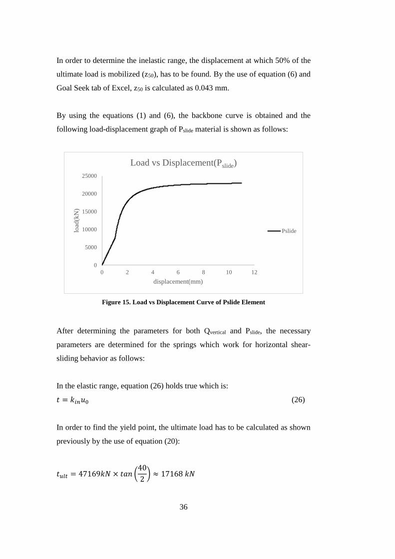
Figure 42. Pier Column Rotation (Single Column Pier versus Multiple Column

Pier, Loose Sand) .............................................................................................. 68

xiii

Figure 43. Pier Column Rotation Ductility (Single Column Pier versus Multiple

Column Pier, Loose Sand) ................................................................................ 68

Figure 44. Footing Vertical Displacement (Single Column Pier versus Multiple

Column Pier, Loose Sand) ................................................................................ 69

Figure 45. Footing Rotation (Single Column Pier versus Multiple Column Pier,

Loose Sand ........................................................................................................ 69

Figure 46. Footing Sliding Displacement (Single Column Pier versus Multiple

Column Pier, Loose Sand) ................................................................................ 70

xiv

1

CHAPTERS CHAPTER 1

1. INTRODUCTION

Soil and structure interaction (SSI) plays a major role in order to model the

structure realistically. SSI could be divided into two divisions as SSI on

buildings and SSI on bridges. SSI in bridges could be divided into three

branches. These are abutment-backfill interaction, soil-pile interaction and

foundation-soil interaction. This thesis mainly focuses on bridges with tall piers

having high aspect ratios to investigate the effects of rocking. Since the effects

of rocking are aimed to be modelled for shallow foundations and high piers, the

effects of sliding are neglected due to the high ratio of pier height to footing

length. Specifically, when the ratio of pier height to footing length becomes less

than 1, sliding dominates the behaviour (Gajan, Kutter, 2009). But this ratio is

much higher in the examples considered in the thesis. The scope of this thesis is

limited to symmetrical bridges having high aspect ratios. For shallow

foundations, rocking effect is important. In order to understand the effects of

rocking, the SSI mechanism is investigated due to the nonlinear behaviour of

soil. This nonlinearity may cause settlement, rotation and sliding. (Gajan, Kutter,

2005) After the observations made in soil-structure interaction field, it is

understood that the subject of soil-structure interaction has to be examined in

earnest. Therefore, it is focused on to create a model in order to illustrate the

effects of cyclic loadings on shallow foundations.

The thesis has two main objectives which are:

First objective is to study rocking on the seismic response of the bridges.

Second objective is to understand the relationship between rotation and

moment of the foundation in order to simulate the behaviour of the

foundation and hysteresis effects.

2

The research mainly focuses on comparative seismic assessment of two bridge

pier types as multi-column pier bent and hammerhead pier for stiff and soil

conditions on shallow foundations. First, an extensive literature review is

conducted. Secondly, soil-structure interaction behaviour of shallow foundations

is explained. Following this explanation, the bridges and parameters used in this

thesis are determined. Following this determination, the bridges are designed and

modelled. After designing and modelling the bridges, the results are analysed.

Then, these analyses are discussed. Finally, the conclusion is made. In the

following sections, these steps are explained in a detailed fashion.

An extensive literature review is conducted on the historical background of soil-

structure interaction, soil-structure interaction modelling and soil-structure

interaction analyses. Based on this information, the necessity of this thesis is

introduced. The information obtained from this literature review is used in order

to model the rocking shallow foundations under cyclic loadings.

Gajan, Kutter, Hutchinson et al. (2007) modelled the shallow foundation under

cyclic loadings by the use of BNWF (Beam on Nonlinear Winkler Foundation)

springs. These springs are used to define the loading, unloading and reloading

phases of the cyclic loading. This model is considered to be the most complete

model since it defines all phases of loading.

To use the moment-rotation backbone curve obtained in Phase 2, BNWF springs

have to be examined in earnest. In this chapter, these springs are introduced and

the properties of them are given. These springs are used to model the medium

dense and dense soil. There are three types of springs which model the soil

according to their densities. Since the structure can undergo displacement in

three ways, namely as in vertical direction and horizontal directions, the springs

are specialized to model the soil-foundation interaction under these three

circumstances. In this chapter, the details of these springs are given.

3

After completing the “Soil-Footing Interaction” Chapter, the bridges are chosen

to be modelled by SAP2000. These bridges are chosen according to their pier

types, span lengths and width of piers.

The design of the bridges is performed in compliance with AASHTO (2014). In

order to complete the design phase, earthquake excitations are chosen from

PEER Ground Motion Database.

Following the design of the bridges, the models of the bridges are created by the

aid of the program in SAP2000. This program is used in order to create the model

by considering various aspects of bridge modelling.

After creating the models of the bridges, the cyclic loadings are applied to the

bridge models. The analyses are obtained from SAP2000.

After analysing the models, the results are discussed in earnest.

The conclusion is made by comparing the seismic performance assessment of

continuous slab on girder bridges with multi-column pier bent and hammerhead

pier for medium dense and dense soil conditions.

5

CHAPTER 2

2. LITERATURE REVIEW

Soil-structure interaction (SSI) is an interdisciplinary field. It is completely

linked with other disciplines as structural mechanics, earthquake engineering

and soil dynamics. This discipline was discovered in late 19th century and it

developed in the beginning of the 20th century. But major developments were

made in the second half of the 20th century thanks to the powerful computers

and programs. These developments are introduced chronologically as follows:

The very first major development was made by Erich Reisner in 1936. He

explored the behaviour of circular discs on elastic half-spaces subjected to time-

harmonic vertical loads. But this exploration did not manage to succeed since he

assumed in his theory that the plate considered in his study had frictionless

contact with the soil. In 1937, he focused on contact shearing stresses which

increased linearly with distance to the axis. Other than Reisner, Sagoci, Apsel,

Luco, Veletsos, Wei and Westmann helped the field to show progression.

In the beginning of 1970s, Veletsos, Luco and Westmann made the invaluable

contribution to the field. The studies of them supplied solutions to the problem

of circular plates underlain by elastic half-spaces excited dynamically over a

wide range of frequencies. After this stage, the needs of nuclear power and

offshore industries shaped the future of soil-structure interaction field.

From the mid-1960s to mid-1970s the powerful computers led the engineers to

work on irregularly shaped foundations embedded in inhomogeneous or layered

media. These developments evolved rapidly with the existence of the programs

such as SHAKE, LUSH, SASSI and CLASSI in this era. In 1978 a heavyweight

6

in SSI field, Dominguez, obtained the impedances of rectangular foundations

embedded in an elastic half space. (Kausel, 2009)

In the beginning of 2000s, the studies got narrowed down due to the specific

industrial needs. The path of SSI field which is going to be followed in the future

entirely relies on the needs of these necessities. All in all, today’s conjecture

shapes the future of this interdisciplinary field.

Soil-structure interaction has an extreme importance to simulate the seismic

response of bridges. Rocking shallow foundations are considered to be

advantageous over fixed-base foundations since they can absorb some of the

ductility demands which would be absorbed by columns. It is observed that

foundations designed for elastic behaviour cannot have these benefits of

nonlinear soil-structure interaction (SSI). Furthermore, it is concluded that

bridge systems with rocking foundations on good soil conditions show small

settlements and good performance (Deng, Kutter, Kunnath, 2012). Moreover,

shallow foundations might be loaded into their nonlinear range during major

earthquake loadings. The nonlinearity of soil might act as an energy dissipation

mechanism and it reduces the shaking demands which are exerted on the

buildings. But if this nonlinearity is not considered, it might cause permanent

deformations and damage to the building (Gajan, Kutter, Phalen et al., 2004). In

case of soil yielding or foundation uplifting, the safety margins of the entire

structure may increase but permanent displacement and rotation might occur

which is totally undesirable (Kokkali, Abdoun, Anastasopoulos, 2015).

Actually, bridge engineers generally depend on the performance of previously

constructed bridges in which the soil-structure interaction (SSI) is not taken into

account. Last but not least, today’s design codes discourage designs which allow

rocking. (Raychowdhury, Hutchinson, 2008)

The models considered in this section take soil-structure interaction modelling

into account. The studies mentioned here consist of models which give

7

correlative results with the corresponding experimental data. However, these

studies do not involve a full cycle which combines both moment-rotation

backbone curves and hysteresis rules in harmony except one. Gajan, Kutter,

Hutchinson et. al (2006) introduced the BNWF (beam on nonlinear Winkler

foundation) springs which model the soil under loading, unloading and reloading

phases. This model is used in the thesis. The details of this model is introduced

to the reader in the following chapter.

One of the biggest problems considered in soil-foundation interaction is rocking.

If the aspect ratio, which is” “, is smaller than 1, sliding dominates the behaviour

(Gajan, Kutter, 2009). But since the models considered in the thesis have aspect

ratios much larger than 1, rocking dominates the behaviour. Ugalde, Kutter,

Jeremic et al. (2007) mentioned the effects of rocking in order to attract

engineers’ attention on rocking. The most important effect of rocking is, rocking

results in lengthening of the natural period that tends to reduce acceleration and

force demands and increase displacement demands on the superstructure. Based

on an entirely different approach, Gajan and Kutter (2009) modelled shallow

foundations subjected to combined cyclic loading. Rocking shallow foundation

model was created by the use of Contact Interface Model (CIM) and the results

of this model showed perfect correlation with the experimental data (p. 9).

Raychowdhury and Hutchinson (2008) created a model to capture the sliding,

settling and rocking movements of a shallow foundation when it was subjected

to earthquake ground motions. This model was developed by the use of Beam-

on-Nonlinear-Winkler-Foundation (BNWF) model which consisted of a system

of uncoupled springs. These springs had nonlinear inelastic behavioural

response. It was stated that, if the amplitude of rocking was acceptable, the

energy sourced by earthquake excitations could be dissipated through soil-

foundation interface with moment-rotation action. The theoretical results were

in very good agreement with the experimental data. Harden, Hutchinson, Martin

et.al (2005) created a numerical model of the nonlinear cyclic response of

shallow foundations. That study was focused on the nonlinear behaviour of

8

shallow building foundations under large-amplitude loading. The model was

based on performance-based earthquake engineering (PBEE). To use PBEE in a

current design, BNWF model was chosen. The experimental results were

compared with theoretical results and they were in very good agreement. Gajan,

Kutter and Thomas (2005) conducted six series of tests in order to study

nonlinear load-deformation characteristics of shallow foundations during cyclic

loading. This nonlinearity was caused by progressive rounding of soil. This led

to a reduction in contact area between footing and soil. Hence, contact element

model was used in this study. Experimental data and the model were compared

and the results were observed to be in very good agreement. Anastasopoulos,

Gelagoti, Kourkoulis et al. (2011) developed a simplified model for the analysis

of the cyclic response of shallow foundations. This study is at the forefront due

to its simplified approach. It was based on the kinematic hardening constitutive

model of Von Mises failure criterion and encoded in ABAQUS. The results were

compared with the experimental data and the results were in very good

agreement.

The studies were carried out on ordinary bridges under earthquake loads with an

entirely new approach called direct displacement-based design (DDBD). A

multilinear model was developed which represented the moment-rotation

backbone curve of the nonlinear moment-rotation behaviour. In addition, an

empirical relationship was proposed that correlated the initial stiffness to the

moment capacity of a rocking foundation. In the design procedure Deng, Kutter

and Kunnath (2014) constructed a bridge system which consisted of a deck mass,

a rocking foundation and a damped elastic column integrated into a single

element. By the use of this model, equivalent linear damping and period could

be determined. DDBD used the equivalent system damping and period along

with a design displacement response spectrum. The results were compared with

theoretical data and it was observed that DDBD produced precise displacement

values.

9

Up to now, the studies considered here captured the moment-rotation backbone

curves by using CIM, BNWF, PBEE and DDBD. The results obtained here show

good correlation with the experimental data. Specifically, the BNWF model is

considered to be the used in the thesis since the unloading and reloading phases

are defined explicitly and thoroughly.

Following the investigation of models which are based on soil-structure

interaction modelling, soil-structure interaction analyses are examined in this

section. The importance of nonlinear soil behaviour was examined and shown

by conducting studies for structures with a constant base and variable height.

Specifically, the importance of SSI increased when soil softens. (Kim, Y.,

Roesset, J.M., 2004). Seismic performance verifications for shallow foundations

were generally assumed to be satisfied but it was understood that the shallow

foundations are generally over-designed (Jiro, F., Masahiro S., Yoshinori, N.,

Ryuichi, A., 2005).

The general consensus is, the increasing number of cycles increases the residual

displacement and stiffness degradation but the moment capacity is not affected

significantly. The common point of the studies considered in this section is, none

of them has a complete hysteresis curve which combines both the moment-

rotation backbone curve and hysteresis rules. In order to understand the

importance of rocking effect on shallow foundations, an extensive literature

review is conducted as follows:

The analyses were done in various aspects. The effect of contact area ratio was

examined by Gajan and Kutter (2008). The studies included several centrifuge

experiments in order to study the rocking behaviour of shallow footings

supported by sand and clay stratums. The tests were conducted during both slow

cyclic loading and dynamic shaking.

10

The importance of soil-structure interaction was not only investigated on

foundation basis. The effects of SSI were investigated on multi-span simply

supported bridges. In order to examine these effects, FHWA’s guidelines for

footing foundation on semi-infinite elastic half space were used to determine

translational and rotational stiffnesses at the base of bridge abutments and piers.

It was concluded that SSI had a detrimental effect specifically on abutments

rather than on the column piers. SSI affected plastic rotation demand and this

demand was higher for medium dense soils rather than soft or stiff soils

(Saadeghvaziri, M.A., Yazdani-Motlagh, A.R., Rashidi, S., 2000).

As it is discussed in section 1.4.1, today’s conjecture shapes the future of SSI.

In this regard, to evaluate the earthquake excitations on the seismic design of a

nuclear containment structure, SSI was examined. The effects were observed by

conducting several centrifuge tests on various soil conditions from loose sand to

weathered rock. Subsoil condition, earthquake intensity and control motion

affected the seismic design of nuclear power plants. It was concluded that soft

soils (sandy and weathered soil) generate less amplification in soil layer and the

period was lengthened more in soft soils compared to rock conditions (Ha, J.,

Kim, D., 2014)

Besides these studies mentioned in this section, kinematic responses of shallow

foundations were studied and the results were tabulated. Based on these results,

it was observed that coupling impedances were considered to be negligible for

shallow foundations. (Mylonakis, G., Nikolaou, S., Gazetas, G., 2006)

Nonlinear behaviour of soil under seismic excitations were examined in various

aspects by conducting 1G large-scale shake table test and cyclic eccentric

loading tests. These aspects varied in loading methods, input seismic motions,

soil densities and the ratio of horizontal and overturning moment loads. This set

of data supplied information related to the model which examined the coupling

effect of horizontal, vertical and overturning loads, the accumulation of residual

11

displacement and the foundation uplift. It was concluded that residual

displacement was dependent on number of loading cycles, the coupling effect of

vertical and horizontal displacement. More importantly, the uplift effect

significantly affected the foundation behaviour in three aspects. These were the

shape of the hysteresis loop, the degradation in rotational stiffness and the

elongation of the vibration property (Shirato, M., Kouno, T., Asai, R. et al.,

2008). Large-scale specimens of sand were constructed and tested under the

cyclic loading imposed on a different shallow foundation model in order to

improve the bearing capacity of soil-foundation systems. The tests were

conducted with medium dense and dense sand examples. The results indicated

that during uplift, the stiffness of the system degraded significantly but as soon

as the eccentric load decreased, the contact area of the soil-foundation system

increased and rocking stiffness recovered (Negro, P., Paolucci, R., Pedretti, S.,

Faccioli E. 2000).

The effects of cyclic loading on rocking shallow foundations were examined in

earnest with increasing numbers of tests. The type of loadings, pier heights, soil

densities were varied and the results were obtained. According to these results,

when the shallow foundation was subjected to cyclic loading, the residual

displacement accumulated with residual rotation and the final residual

displacement was entirely dependent on numbers of cycles, loading patterns and

soil densities (Jiro, F., Masahiro, S., Yoshinori, N., Ryuichi, A., 2005).

Another aspect of rocking shallow foundations was considered under cyclic

loadings. Since it was aimed to ensure that rocking was materialized through

uplifting rather than sinking, a large vertical factor of safety (FSv) was required

but since the soil properties could not be foreseen, this application was

considered to be feasible in theory. Since rocking-induced soil yielding was only

mobilized within a shallow layer underneath the footing, “shallow soil

improvement” was considered to eliminate the risks of unforeseen inadequate

FSv. It was ensured that, with aspect ratios larger than 1, rocking dominated

12

sliding in the experiments. It was concluded in these series of tests that if the

depth of the foundation was equal to the width of the foundation, shallow soil

improvement could be effective. Last but not least, it was stated that increasing

numbers of cycles alter the effectiveness of shallow soil improvement

(Anastasopoulos, I., Kourkoulis, R., Gelagoti, R., et al. 2012).

The studies mentioned above, take soil-structure interaction into account in the

modelling phase. But as mentioned in this section, BNWF springs are considered

to be the most complete model in the design phase. Gajan, Hutchinson, Kutter et

al. (2007) explained the properties of BNWF model. This model is considered

to be the most complete model since it explains the elastic and plastic behaviour

of soil in loading, unloading and reloading phases. Moreover, horizontal and

vertical displacement of soil are taken into account in the same model.

13

CHAPTER 3

3. DESCRIPTION OF THE BRIDGES USED IN THE ANALYSES

In this chapter, description of the bridges is introduced to the reader. The reasons

why Eskişehir Köseköy Bridge is used in the analyses are explained in earnest.

In order to compare the seismic effects on continuous slab on girder bridges with

multi-column pier bent and hammerhead pier, the bridges constructed in real life

are examined. KMG, Inpro and Yuksel Project played a significant role in this

part of the thesis since these three firms supplied the bridges constructed

according to the research field of the thesis.

The survey mentioned in “Choice of Bridges” consists of 44 bridges. 13 of these

bridges have multi-column head piers and 31 of them have hammerhead piers.

They are designed for 0.3g-0.4g peak ground acceleration. The survey includes

prestressed and post-tensioned bridges. These bridges are mainly categorized

under two branches according to their pier types which are multi-column pier

bent and hammerhead pier. The related aspect ratios of these piers in both lateral

and transverse directions are tabulated. Furthermore, to model these bridges

realistically, same study is carried out for the left and right abutments of these

bridges.

In tables 3.1, 3.2, 3.3 and 3.4, the aspect ratios of the bridges in this study are

taken into consideration.

Table 3.1. Aspect Ratio Results of Multi-Column Pier Bent (h/B)

ASPECT RATIO RESULTS (h/B)

MAX MIN AVERAGE ST DEV

1.669 0.567 1.185 0.241

14

Table 3.2. Aspect Ratio Results of Multi-Column Pier Bent (h/L)

ASPECT RATIO RESULTS (h/L)

MAX MIN AVERAGE ST DEV

3.000 0.311 1.078 0.860

Table 3.3. Statistical Results of the Distribution of the Aspect Ratios(h/B)

(h/B) # of data AR %

0.5-

1.0(0.756) 3 0.756 10.71

1.0-

1.5(1.202) 24 1.102 85.71

1.5-

2.0(1.624) 2 1.624 7.14

Table 3.4. Statistical Results of the Distribution of the Aspect Ratios(h/L)

(h/L) # of data AR %

0-0.5(0.445) 13 0.44 46.43

0.5-

1.0(0.721) 7 0.721 25.00

1.0-1.5(1.25) 1 1.25 3.57

1.5-

2.0(1.833) 1 1.833 3.57

2.0-

2.5(2.302) 4 2.302 14.29

2.5-

3.0(2.597) 2 2.597 7.14

3.0-

3.5(3.000) 1 3 3.57

The values in parenthesis under “h/B” and “h/L” columns indicate the average

values of aspect ratios in their current range. For instance, 3 samples of h/B data

have an aspect ratio, varying in between 0.5 and 1.0. The average of these three

samples equals 0.756. Here, “B” stands for the breadth of the foundation and

“L” stands for the length of the foundation.

15

Figure 1. Frequency vs Aspect Ratios of Multi-Column Pier Bent (h/B)

Figure 2. Frequency vs Aspect Ratios of Multi-Column Pier Bent (h/L)

Table 3.5. Aspect Ratio Results of Hammerhead Pier (h/B)

ASPECT RATIO RESULTS (h/B)

MAX MIN AVERAGE ST DEV

3.800 0.442 1.663 0.604

Table 3.6. Aspect Ratio Results of Hammerhead Pier (h/L)

ASPECT RATIO RESULTS (h/L)

MAX MIN AVERAGE ST DEV

3.470 0.447 1.514 0.589

0.00

20.00

40.00

60.00

80.00

100.00

0.5-1.0(0.756) 1.0-1.5(1.202) 1.5-2.0(1.624)

Fre

quen

cy(%

)

Aspect Ratio

Frequency (%) vs Aspect Ratio(multi-column

head,pier,h/B)

0.00

10.00

20.00

30.00

40.00

50.00

Fre

quen

cy(%

)

Aspect Ratio

Frequency (%) vs Aspect Ratio(multi-column

head,pier,h/L)

16

Table 3.7. Statistical Results of the Distribution of the Aspect Ratios (h/B)

h/B # of data AR %

0-0.5(0.442) 1 0.442 0.51

0.5-1.0(0.822) 26 0.822 13.33

1.0-1.5(1.231) 52 1.231 26.67

1.5-2.0(1.746) 63 1.746 32.31

2.0-2.5(2.194) 34 2.194 17.44

2.5-3.0(2.704) 15 2.704 7.69

3.0-3.5(3.045) 2 3.045 1.03

3.5-4.0(3.661) 2 3.661 1.03

Table 3.8. Statistical Results of the Distribution of the Aspect Ratios (h/L)

h/L # of data AR %

0-0.5(0.472) 2 0.472 1.03

0.5-1.0(0.801) 40 0.801 20.51

1.0-1.5(1.226) 57 1.226 29.23

1.5-2.0(1.701) 52 1.701 26.67

2.0-2.5(2.221) 32 2.221 16.41

2.5-3.0(2.672) 11 2.672 5.64

3.0-3.5(3.47) 1 3.47 0.51

Figure 3. Frequency vs Aspect Ratios of Hammerhead Pier (h/B)

0.00

5.00

10.00

15.00

20.00

25.00

30.00

35.00

Frequency(%) vs Aspect

Ratio(hammerhead,pier,h/B)

17

Figure 4. Frequency vs Aspect Ratios of Hammerhead Pier (h/L)

Under the light of these analyses, Eskişehir Köseköy Bridge is chosen for

modelling. The aspect ratios of the piers of Eskişehir Köseköy Bridge in

longitudinal direction are 1.619, 1.769 and 1.763. These results comprise of 32%

of the total range as shown on the previous chart. Moreover, the aspect ratios of

the same bridge in transverse direction are found as 1.295, 1.415 and 1.410.

These results comprise of almost 27% of the total range as shown on the previous

chart. Hence Eskişehir Köseköy Bridge is considered to be a common bridge in

terms of its aspect ratios.

Eskişehir Köseköy Bridge has equal spans with 32 meters. In the thesis, three

spans of this bridge are modelled including its abutment and the foundations of

both abutment and piers. Since it is considered to model the bridge under

earthquake excitation with dense, medium dense and loose sand, the foundations

are designed by the coefficients of Meyerhof and Brinch-Hansen (Salgado,

2003).

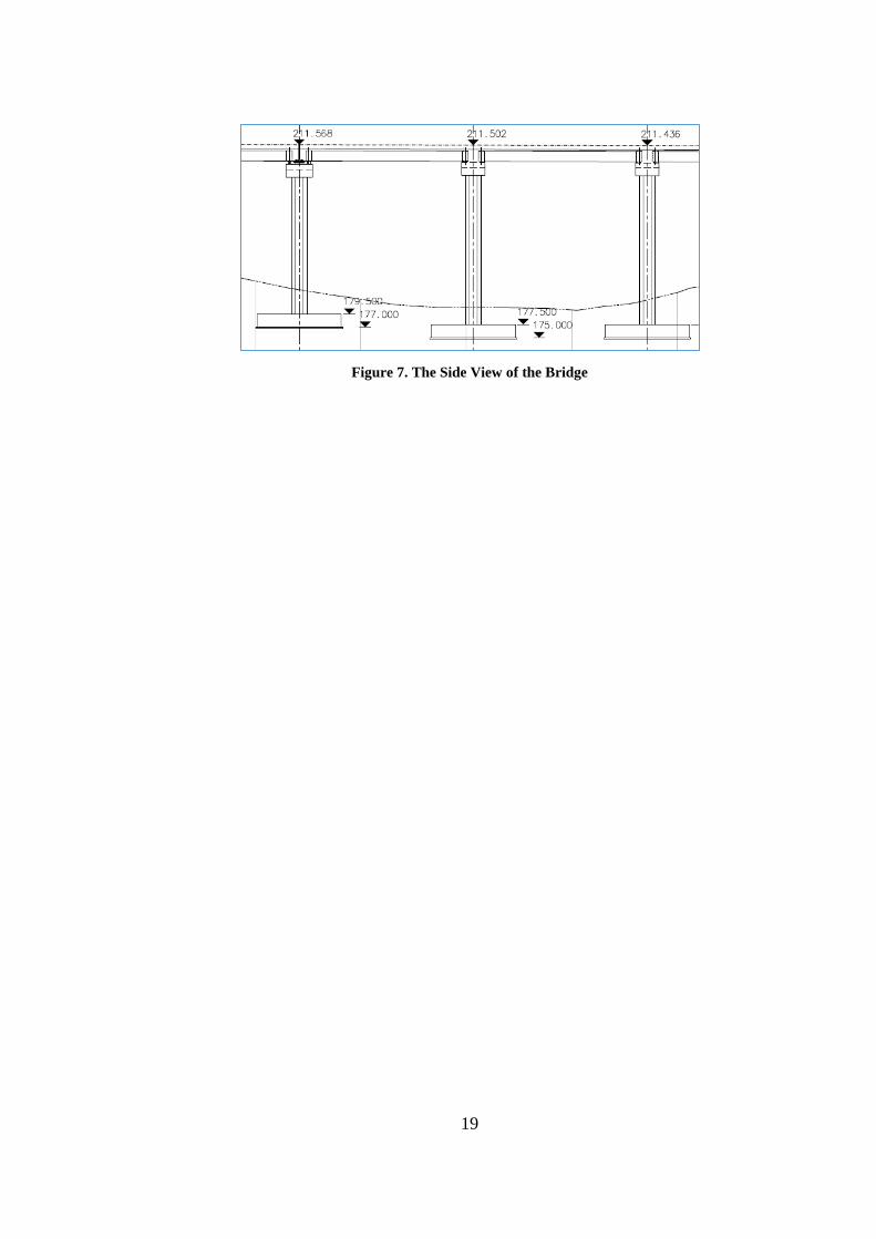
Köseköy Bridge is a railway bridge. The width of this bridge is 12 meters. It has

two lanes. Figures 5,6, and 7 give an overview related to the bridge considered

in this study.

0.00

5.00

10.00

15.00

20.00

25.00

30.00

35.00

Frequency(%) vs Aspect

Ratio(hammerhead,pier,h/L)

18

Figure 5. Cross Sectional View of Köseköy Bridge

Figure 6. The Side View of the Abutment

19

Figure 7. The Side View of the Bridge

21

CHAPTER 4

4. FOUNDATION SOIL PARAMETERS USED IN THE DESIGN FOR

VARIOUS SOIL TYPES

In this chapter, the parameters used in the design for modelling the soil are

introduced. After this introduction, the Beam on Nonlinear Winkler Foundation

(BNWF) model is introduced.

Three types of soil stiffnesses are used in order to observe the effects of rocking.

Bowles (1997) classified the soil as very loose, loose, medium, dense and very

dense. In this thesis, loose, medium and dense sand types are taken into

consideration.

Table 4.1. . Properties of Sand Types Considered in This Study (Bowles,1997)

Description Very

Loose

Loose Medium Dense Very

Dense

Relative

Density,Dr

0 0.15 0.35 0.65 0.85

Φfine 26-28 28-30 30-34 33-38 <50

Φmedium 27-28 30-32 32-36 36-42 <50

Φcoarse 28-30 30-34 33-40 40-50 <50

γwet

(kN/m3)

11-16 14-18 17-20 17-22 20-23

22

Table 4.2. Soil Properties Used in This Study from FHWA (1997), AASHTO(2014) and

Bowles (1997)

Soil Type γ1 (kN/m3) N2 Gmax(2)

(kPa)

Vs,(2) (m/s) AASHTO

Soil

Class(3)

Dense

Sand

20 40 224000 330 D

M. Dense

Sand

18 18 118000 250 D

Loose

Sand

16 7 55000 150 E

Density values are tabulated form Bowles (1997), shear modulus values and the

shear wave velocities are tabulated from FHWA (1997) and soil classes are taken

from AASHTO(2014).

After introducing the necessary parameters for the soil types considered in this

thesis, BNWF Model is introduced as follows:

BNWF model is developed for a 2D-analysis. Hence 1D elastic beam column

elements have 3 DoF’s per node as horizontal, vertical and rotation. Individual

1D zero-length springs are independent of each other with nonlinear inelastic

behavior modeled using modified versions of Qzsimple1, Pysimple1 and

Tzsimple1.

Qzsimple1 simulates vertical load-displacement behavior. Pysimple1 simulates

horizontal passive load-displacement behavior against the side of a footing and

Tzsimple1 simulates the horizontal shear-sliding behavior at the base of the

footing.

23

The schematic view below represents the locations of the springs. Vertical

springs are distributed along the footing. Horizontal springs are located along

both the short and long edge of the footing in order to capture shear and sliding

behavior.

Figure 8. Beam on Nonlinear Winkler Foundation (BNWF) Schematic View

Furthermore the model mentioned above can capture hysteretic energy

dissipation and account for radiation damping at the foundation base. All three

types of springs are characterized by a nonlinear backbone curve, resembling a

bilinear behavior. The bilinear curve consists of a linear and a nonlinear region

with gradually decreasing stiffness as displacement increases. For Pysimple1

and Tzsimple1 springs, an ultimate load is defined for both tension and

compression. Qzsimple1 springs have a reduced strength in tension to account

for soil’s limited tensile capacity. The working mechanism of the QzSimple1

material is explained in Figure 9. This material is spotted with a circle in Figure

8.

24

Figure 9. Typical zero length spring (proposed model)

Elastic and plastic components are added in series via gap elements in the

proposed model created by Gajan, Kutter et al.(2008). The gap component of the

spring is a parallel combination of a closure and a drag spring. The closure

component is a bilinear elastic spring which is relatively rigid in compression

and very flexible in tension. For shallow foundations, a single spring is used

since the footing is assumed to be rigid with respect to shear and flexural

deformations over its height.

The model considered in the thesis is more simplistic and gives realistic results.

Instead of connecting the damper and elastic spring in parallel, every member

is linked in series.

25

Figure 10. Nonlinear Backbone Curve for Qzsimple1 material

This backbone curve consists of two regions which are elastic region and

inelastic region. The formulae which govern these regions are given as follows:

In the elastic region:

𝑞 = 𝑘𝑖𝑛𝑧 (1)

𝑞0 = 𝐶𝑟𝑞𝑢𝑙𝑡 (2)

The elastic stiffness values are obtained from Gazetas (1991):

In vertical direction;

𝑘𝑧 =𝐺𝐿

1−𝜈[0.73 + 1.54 (

𝐵

𝐿)

0.75

] (3)

In horizontal direction (toward long side of the footing);

𝑘𝑦 =𝐺𝐿

2−𝜈[2 + 2.5 (

𝐵

𝐿)

0.85

] (4)

In horizontal direction (toward short side of the footing);

𝑘𝑥 =𝐺𝐿

2−𝜈[2 + 2.5 (

𝐵

𝐿)

0.85

] +𝐺𝐿

0.75−𝜈[0.1 (1 −

𝐵

𝐿)] (5)

The formula which holds true for the nonlinear region is given as follows:

𝑞 = 𝑞𝑢𝑙𝑡 − (𝑞𝑢𝑙𝑡 − 𝑞0) [𝑐𝑧50

𝑐𝑧50+|𝑧−𝑧0|]

𝑛

(6)

z50: displacement where 50% of the total displacement is mobilized

z0: displacement at the yield point

26

The equations derived above are valid for Qzsimple1, Pysimple1 and Tzsimple1

springs.

By the use of the equations mentioned above, the gapping capabilities of

Qzsimple1 and Pysimple1 springs, the reduced tensile strength of Qzsimple1

spring and the hysteresis of the sliding resistance (without gapping) of

Tzsimple1 spring are shown as follows:

Figure 11. Cyclic response of uni-directional zero-length spring models: (a) axial load-

displacement response, (b) lateral passive response (Pysimple1 material), (c) lateral

sliding response (Tzsimple1 material)

The parameters given in equations (1), (2) and (3) have to be identified. Since

sand is taken into consideration, the cohesion parameter, c is equal to zero

whereas the internal angle of friction is not equal to 0.

In order to capture the behavior of Qzsimple1, Pysimple1 and Tzsimple1

springs, the following equations are derived as follows:

The ultimate bearing capacity of a Qvertical spring is given in equation (7).

𝑞𝑢𝑙𝑡 = 𝑐𝑁𝑐𝐹𝑐𝑠𝐹𝑐𝑑𝐹𝑐𝑖 + 𝛾𝐷𝑓𝑁𝑞𝐹𝑞𝑠𝐹𝑞𝑑𝐹𝑞𝑖 + 0.5𝛾𝐵𝑁𝛾𝐹𝛾𝑠𝐹𝛾𝑑𝐹𝛾𝑖 (7)

For sand, c equals zero which is the cohesive intercept. Hence the first part of

the summation is cancelled out. The equations for each factor given in Equation

(7) are derived by Salgado (2006):

27

It has to be stated that the parameters in equation (7), are used from both

Meyerhof (2006) and Brinch-Hansen (2006).

γ: soil unit weight;

Df: embedment;

𝑁𝑞 =1+𝑠𝑖𝑛∅

1−𝑠𝑖𝑛∅𝑒𝜋𝑡𝑎𝑛∅ (8)

Nq: bearing capacity factor for soil surcharge (unitless)

φ: friction angle;

𝐹𝑞𝑠 = (1 +𝐵

𝐿× 𝑠𝑖𝑛∅) (9)

N: flow number;

𝑁 =1+𝑠𝑖𝑛∅

1−𝑠𝑖𝑛∅ (10)

𝐼𝑓𝐷

𝐵≤ 1; 𝐹𝑞𝑑 = 1 + 2 × 𝑡𝑎𝑛∅ × (1 − 𝑠𝑖𝑛∅)2 ×

𝐷

𝐵 (11)

𝐼𝑓 𝐷

𝐵> 1; 𝐹𝑞𝑑 = 1 + 2 × 𝑡𝑎𝑛∅ × (1 − 𝑠𝑖𝑛∅)2 × 𝑡𝑎𝑛−1 𝐷

𝐵 (12)

B: breadth, D: depth within a soil mass;

𝐹𝑞𝑖 = [1 −𝑎𝑟𝑐𝑡𝑎𝑛(

𝑄𝑡𝑟𝑄𝑎𝑥

)

900 ]

2

(13)

arctan(Qtr/Qax): inclination angle of the load

𝑁𝛾 = 1.5(𝑁𝑞 − 1)𝑡𝑎𝑛∅ (14)

𝐹𝛾𝑠 = 1 − 0.4𝐵

𝐿 (15)

𝐹𝛾𝑑 = 1

Nγ: bearing capacity factor for unit weight term (unitless)

𝐹𝛾𝑖 = [1 −𝑎𝑟𝑐𝑡𝑎𝑛(

𝑄𝑡𝑟𝑄𝑎𝑥

)

∅]

2

(16)

The working mechanism of the spring which simulates the passive load-

displacement behavior against a footing is given as follows:

𝑝𝑢𝑙𝑡 = 0.5𝛾𝐷𝑓2𝐾𝑝 (17)

Kp: passive earth pressure coefficient. In this work, Coulomb’s expression is

used. That expression is given as follows:

28

𝐾𝑝 =𝑠𝑖𝑛2(𝛽−∅)

𝑠𝑖𝑛2𝛽𝑠𝑖𝑛(𝛽+𝛿)[1−√𝑠𝑖𝑛(∅+𝛿)𝑠𝑖𝑛(∅+𝛼)

𝑠𝑖𝑛(𝛽+𝛿)𝑠𝑖𝑛(𝛽+𝛼)]

2 (18)

Kp can be expressed by Rankine’s derivation. That derivation is more simplistic

than Coulomb’s expression which is mentioned below:

𝐾𝑝 = 𝑡𝑎𝑛2 (45 +∅

2) (19)

The mechanism of springs which illustrate the shear-sliding behavior is given

as:

t𝑢𝑙𝑡 = 𝑊𝑔𝑡𝑎𝑛𝛿 + 𝐴𝑏𝑐 (20)

Wg: vertical force acting at the base of the foundation

δ: angle of friction between the foundation and soil (typically varying from 1

3∅

to 2

3∅).

Ab: area of the base of the footing in contact with the soil

c: cohesion intercept ( It is zero for sand.)

After determining the formulae which govern the elastic and plastic regions of

the springs, the end length ratio and the stiffness intensity ratio parameters are

given as follows:

Stiffness Intensity Ratio, 𝑅𝑘 =𝑘𝑒𝑛𝑑

𝑘𝑚𝑖𝑑 (21)

End Length Ratio, 𝑅𝑒 =𝐿𝑒𝑛𝑑

𝐿 (22)

Lend: length of the edge region over which the stiffness is increased. Lend is

recommended as B/6 by ATC-40. This length can be determined from the

following figure:

29

Figure 12. End length ratio versus footing aspect ratio

Stiffness Intensity Ratio can be determined from the following figure:

Figure 13. Stiffness intensity ratio versus footing aspect ratio

Spring spacing: 𝑠 =𝑙𝑒

𝐿. Minimum number of 25 springs is recommended.

L: footing length

le: length of the footing element

Initial unloading stiffness is equal to initial loading stiffness.

The stiffness of the elastic range can be derived from Equation (1). It is defined

by Cr. The stiffness of the plastic range can be derived from Equation (3) as

follows:

𝑘𝑝 = 𝑛(𝑞𝑢𝑙𝑡 − 𝑞0) [(𝑐𝑧50)𝑛

(𝑐𝑧50−𝑧0+𝑧)𝑛+1] (23)

30

Following table shows the values of Cr, c and n which are constitutive parameters

to determine the limits of elastic and plastic range:

Table 4.3. Nonuser defined parameters (Raychowdhury and Hutchinson, 2008)

Material

Type

Soil

Type

References Values Used in the Current

Study

Cr n c

QzSimple1 Sand Vijayvergiya(1977) 0.36 5.5 9.29

PySimple1 Sand API(1993) 0.33 2 1.1

TzSimple1 Sand Mosher(1984) 0.48 0.85 0.26

Concluding Remarks:

Rk (end stiffnes ratio) affects the permanent settlement significantly. On

the other hand, its effect on maximum rotation and maximum stiffness is

too slight.

Re (end length ratio) has a modest effect on the shape of the settlement-

rotation and moment-rotation curve and nominally on total settlement.

A smoother footing response occurs when a great number of springs are

used.

A larger Cr extends the elastic region, reduces the total settlement for a

given load. A smaller Cr increases the total settlement.

Constitutive parameter, c, affects the nonlinear portion of rotational

stiffness and settlement significantly.

Reducing the unloading stiffness to 20% of the loading stiffness, only

increases the settlement by 6%.

As mentioned above, the unloading load-displacement curve is identical

in shape to the loading curve.

After the explanation of QzSimple1, PySimple1 and TzSimple1 materials, the

nonlinear backbone curves of these materials are obtained. In this thesis, the

names of these materials are changed in order to prevent confusion. The springs

31

which work vertically are labeled as Qvertical. The springs which slide and shear

are labeled as Qslide and Qshear, respectively.

The project consists of comparative seismic assessment of bridges under loose

to stiff soil conditions. First, the spring properties of Eskişehir Köseköy Bridge

are determined under dense soil conditions for Qvertical, Qslide and Qshear materials.

After determination of these properties, the same project is examined under

medium dense conditions for these three materials. The parameters of these

bridges considered in this study are given in the table as shown:

Table 4.4. Parameters of the bridges considered in this study

Eskişehir

Köseköy Bridge

(under dense

sand conditions)

Eskişehir

Köseköy Bridge

(under medium-

dense sand

conditions)

Eskişehir

Köseköy Bridge

(under loose

sand conditions)

γ(kN/m3)

(dense/medium

dense)

20 18 16

Df (m) 6 6 6

B (m) 10 11 11

L (m) 14 14 15

Φ

(dense/medium

dense)

40 35 30

As an example, the backbone curves of the springs under dense sand conditions

are obtained as follows:

The friction angle of soil is taken as 400 for dense sand.

The density of dense sand is 20 kN/m3. (Bowles, 1996)

The embedment is taken by 6 meters.

By the use of the formulae mentioned in the previous section, the

necessary parameters to calculate the bearing capacity under both elastic

and inelastic regions are found as follows:

Equation (2) states that;

32

𝑞0 = 𝐶𝑟𝑞𝑢𝑙𝑡 where q0 and Cr stand for the load at the yield point and a

constitutive parameter, respectively. After passing the yield point, the

inelastic range starts.

The constitutive parameter Cr is taken as 0.36 from Table 1. The ultimate bearing

capacity is calculated by the use of the equation (7):

In equation (7), the cohesion parameter, c is equal to zero. Since sand is a

cohesionless material, the first term in the equation equals zero. The angle of

friction, density of dense sand and embedment depth are given in the previous

section. In order to calculate the ultimate bearing capacity, the flow number, N,

has to be calculated. The value of flow number is calculated as follows:

𝑁 =1 + 𝑠𝑖𝑛40

1 − 𝑠𝑖𝑛40≈ 4.60

After calculating the flow number, transverse and axial loads which are resisted

by the pier are calculated. These values are 8654 kN abd 47169 kN, respectively.

The values obtained here are used in the formula mentioned as follows:

𝑞𝑢𝑙𝑡 = 20 × 6 ×1 + 𝑠𝑖𝑛40

1 − 𝑠𝑖𝑛40𝑒𝜋𝑡𝑎𝑛40 × (1 +

10

14× 𝑠𝑖𝑛40)

× [1 + (2 × 𝑡𝑎𝑛∅ × (1 − 𝑠𝑖𝑛∅)2) ×6

10]

× [1 −𝑡𝑎𝑛−1 8654

4716990

]

2

+ 0.5 × 20 × 10

× 1.5(𝑁𝑞 − 1) tan(40) × (1 − 0.4 ×10

14) × 1

× [1 −𝑡𝑎𝑛−1 8654

47169∅

]

2

≈ 13035.2 𝑘𝑁/𝑚2

The value found above as the ultimate bearing pressure for the foundation is

multiplied by the area of the foundation and divided into 25 since the soil is

33

modelled by the use of 25 vertical springs and the force-deformation relationship

of these springs are obtained.

𝐹𝑠𝑝𝑟𝑖𝑛𝑔,𝑣𝑒𝑟𝑡𝑖𝑐𝑎𝑙 = 𝑞𝑢𝑙𝑡 ×10 × 14

25≈ 72997𝑘𝑁

𝑞0 = 0.36 × 72997 ≈ 26279 𝑘𝑁

Up until the loading values reach q0, Qvertical material behaves elastically. The

elastic region of the backbone curve is determined by equation (1):

𝑞 = 𝑘𝑖𝑛𝑧

At this stage, the stiffness value in the elastic range has to be computed in order

to draw the elastic portion of the backbone curve. Gazetas’ equation (1991) is

given as follows in order to determine the vertical stiffness of the mechanistic

springs:

𝐾𝑧 =𝐺𝐿

1 − 𝜈[0.73 + 1.54 (

𝐵

𝐿)

0.75

]

The shear modulus value of the dense sand is used as 224,000 kPa from table

4.2.

After the determination of shear modulus, the foundation stiffness of vertical

springs is calculated as follows:

𝐾𝑧 =224 × 103 × 14

1 − 0.35[0.73 + 1.54 (

10

14)

0.75

] ≈ 9294.8 𝑘𝑁/𝑚𝑚

𝑧0 =𝑞0

𝐾𝑧≈ 146.7 𝑚𝑚

After determining the elastic range of the backbone curve, the necessary steps

are followed to draw the inelastic region of the backbone curve. Since the

34

ultimate bearing capacity is calculated in the previous step by the use of equation

(7), it is not re-calculated again.

There is only one missing parameter in equation (6) which is z50. It stands for

the displacement at which 50% of the ultimate load is mobilized. Since the

ultimate load, the load at the yield point, the constitutive parameters, c and n, are

determined, z50 is calculated by rearranging the terms of equation (6) as follows:

𝑞50 = 𝑞𝑢𝑙𝑡 − (𝑞𝑢𝑙𝑡 − 𝑞0) [𝑐𝑧50

𝑐𝑧50 + |𝑧50 − 𝑧0|]

𝑛

𝑞50 =𝑞𝑢𝑙𝑡

2≈ 36499𝑘𝑁

From the equation above, by the use of Goal Seek feature of Excel, z50 is

calculated as 255 mm.

Since the parameters to draw the elastic and inelastic regions of the backbone

curve are determined, the following load vs displacement curve of Qvertical

material is obtained as follows:

Figure 14. Load vs Displacement Curve of Qvertical Element

0

10000

20000

30000

40000

50000

60000

70000

0 200 400 600 800 1000 1200

load

(kN

)

displacement(mm)

Load vs Displacement (Qvertical)

Qvertical

35

After determining the necessary parameters for the springs which work

vertically, the springs which work for horizontal passive load-displacement

behavior are explained below:

In the elastic range, equation (24) holds true which is:

𝑝 = 𝑘𝑖𝑛𝑢 (24)

This time, equation (1) is used to calculate lateral displacement. The load at the

yield point, p0 is calculated by the use of equation (24).

𝑝𝑢𝑙𝑡 = 0.5𝛾𝐷𝑓2𝐾𝑝 (25)

𝑝𝑢𝑙𝑡 = 0.5 × 20 × 62 × 𝑡𝑎𝑛2 (45 +40

2) ≈ 1655.6 𝑘𝑁/𝑚

These springs work in lateral direction and model the passive pressure of the

soil. Two Pslide springs are used in this model and they are locaed on both sides

of the foundation. The force of a single spring is calculated by multiplying the

ultimate passive pressure by the length of the footing.

𝐹𝑠𝑝𝑟𝑖𝑛𝑔,𝑠𝑙𝑖𝑑𝑒 ≈ 23178.5 𝑘𝑁

𝑝0 = 𝐶𝑟 × 𝑃𝑢𝑙𝑡 = 0.33 × 23178.5 ≈ 7648.9 𝑘𝑁

At this point, the elastic stiffness parameter of Pslide material has to be found by

the use of equation (5) in order to draw the elastic portion of the backbone curve.

𝐾𝑥 =224 × 14 × 103

2 − 0.35× [2 + 2.5 (

10

14)

0.85

]

𝐾𝑥 = 7370.8 𝑘𝑁/𝑚𝑚

𝑢0 =𝑝0

𝑘𝑖𝑛=

7648.9

7370.8≈ 1.038𝑚𝑚

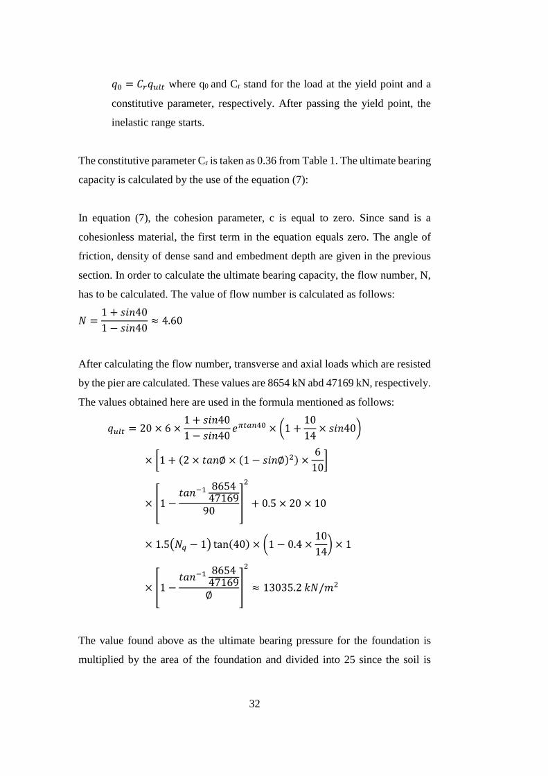
36

In order to determine the inelastic range, the displacement at which 50% of the

ultimate load is mobilized (z50), has to be found. By the use of equation (6) and

Goal Seek tab of Excel, z50 is calculated as 0.043 mm.

By using the equations (1) and (6), the backbone curve is obtained and the

following load-displacement graph of Pslide material is shown as follows:

Figure 15. Load vs Displacement Curve of Pslide Element

After determining the parameters for both Qvertical and Pslide, the necessary

parameters are determined for the springs which work for horizontal shear-

sliding behavior as follows:

In the elastic range, equation (26) holds true which is:

𝑡 = 𝑘𝑖𝑛𝑢0 (26)

In order to find the yield point, the ultimate load has to be calculated as shown

previously by the use of equation (20):

𝑡𝑢𝑙𝑡 = 47169𝑘𝑁 × 𝑡𝑎𝑛 (40

2) ≈ 17168 𝑘𝑁

0

5000

10000

15000

20000

25000

0 2 4 6 8 10 12

load

(kN

)

displacement(mm)

Load vs Displacement(Pslide)

Pslide

37

𝑡0 = 𝐶𝑟 × 𝑡𝑢𝑙𝑡 = 0.48 × 17168 ≈ 8240.7 𝑘𝑁

𝐾𝑦 =224 × 14 × 103

2 − 0.35[2 + 2.5 (

10

14)

0.85

] +224 × 14 × 103

0.75 − 0.35[0.1 × (1 −

10

14)]

𝐾𝑦 = 7594.8 𝑘𝑁/𝑚𝑚

𝑢0 =8240.7

7594.8≈ 1.085𝑚𝑚

In order to determine the inelastic range, the displacement at which 50% of the

ultimate load is mobilized (z50), has to be found. By the use of equation (6) and

Goal Seek tab of Excel, z50 is calculated as 1.1 mm approximately.

By using the equations (1) and (6), the backbone curve is obtained and the

following load-displacement graph of TzSimple1 material is shown as follows:

Figure 16. Load vs Displacement Curve of Tshear Element

0

5000

10000

15000

20000

0 20 40 60 80 100 120

load

(kN

)

displacement(mm)

Load vs Displacement (Tshear)

Tshear

39

CHAPTER 5

5. MODELLING OF THE BRIDGES

In this chapter, the modelling phases of the foundation, aubtment and the piers

are introduced. Eskişehir Köseköy Bridge is the benchmark bridge according to

the statistical analyses conducted in this thesis. In order to observe the effects of

rocking,the foundations of the piers are changed.

First, the modelling phase of the foundation is explained. After this explanation,

the simplistic design of the abutment is explained. In the last step, the design of

multiple column pier bent is explained to the reader.

5.1. Modeling of the Foundation

The original bridge has identical foundations with the dimensions of 16 meters

to 20 meters. But since the effect of rocking is studied in this thesis, the footings

are changed according to the formulae of Meyerhof, and Brinch Hansen

(Salgado,2003).

For dense, medium dense and loose sand types, three different foundation

dimensions are calculated.

In order to design the foundation, the capacity design is made. In this step, the

ultimate bearing capacity of the foundation has to be calculated. This calculation

is done by the formulae of Meyerhof and Brinch Hansen. (Salgado,2003)

Before heading into the chart which gives the value of the ultimate pressure of

the foundation, necessary parameters and the formulae are explained as follows:

40

Bearing capacity of the footings in sand can be calculated by the formulae of

Meyerhof and Brinch Hansen. In this study, a hybrid formula is used which

contains multipliers from both of the formulae. Since Meyerhof’s formula is

upgraded by the experiments conducted in the field, new parameters are taken

from Brinch Hansen’s formula.

The friction angle values for dense, medium dense and loose sand conditions are

used as 400,350 and 300, respectively (FHWA,1986).

The flow number, N, is calculated as follows:

𝑁 =1+𝑠𝑖𝑛∅

1−𝑠𝑖𝑛∅ (27)

Bearing capacity factor, Nq, is obtained by the use of the flow number as follows:

𝑁𝑞 =1+𝑠𝑖𝑛∅

1−𝑠𝑖𝑛∅𝑒𝜋𝑡𝑎𝑛∅ (28)

Since these calculations are done for dense sand, friction angle, φ, is taken as

400. Hence, N equals 4.6.

After the calculation of N, the shape, depth and inclinations factors are taken into

consideration. Shape and depth factors, sq and dq respectively, are calculated by

the formula of Brinch Hansen whereas the inclination factor is calculated by the

formula of Meyerhof.

𝑠𝑞 = 1 +𝐵

𝐿𝑠𝑖𝑛∅ (29)

In the shape factors, the breadth value is not equal to the actual value of 10 meters

under dense sand conditions. In capacity design, the dimensions “B” and “L” are

determined by the direction of loading. In transverse loading conditions, the

dimension “B” is equal to 1.27 meters and the longitudinal direction is equal to

10 meters.

41

If D/B, which is the ratio of the depth of the foundation to the breadth of the

footing, is smaller than 1, the following formula governs for the depth factor:

𝑑𝑞 = 1 + 2𝑡𝑎𝑛∅(1 − 𝑠𝑖𝑛∅)2 𝐷

𝐵 (30)

If D/B is larger than 1, the following formula governs:

𝑑𝑞 = 1 + 2𝑡𝑎𝑛∅(1 − 𝑠𝑖𝑛∅)2𝑡𝑎𝑛−1 𝐷

𝐵 (31)

The inclination factor, iq , is given as follows:

𝑖𝑞 = [1 −𝑎𝑟𝑐𝑡𝑎𝑛(

𝑄𝑡𝑟𝑄𝑎𝑥𝑖𝑠𝑙

)

90]

2

(32)

The inclination factor consists of two parameters which are the transverse

loading and the axial loading. Transverse loading is the summation of two

components. First component is obtained by dividing the plastic moment

capacity into the total height of the pier, cap beam and pedestal. Second

component is the footing inertial force which is calculated from the

mutliplication of the weight of the footing by the peak ground acceleration which

is equal to 0.35.

Table 5.1. Ultimate Bearing Capacity of The Footing Under Dense Sand Conditions

CAPACITY DESIGN OF THE FOUNDATION (DENSE SAND)

Density (kN/m3) 20

Depth of the Foundation (Df,m) 6

Angle of Friction (φ) 40

Nq 64.2

N 4.6

B(m) 1.27

L(m) 10

Fqs 1.081

Fqd 1.292

Fqi 0.694

Nγ 79.5

Fγs 0.95

Fγd 1

Fγi 0.39

qult (kPa) 7842

42

Same procedure is followed in the calculation phases of the capacity design of

the foundations under medium dense and loose sand conditions. The results are

tabulated as follows:

Table 5.2. Ultimate Bearing Capacity of The Footing Under Medium Dense Sand

Conditions

CAPACITY DESIGN OF THE FOUNDATION (MEDIUM DENSE SAND)

Density (kN/m3) 18

Depth of the Foundation (Df,m) 6

Angle of Friction (φ) 35

Nq 33.3

N 3.69

B(m) 1.54

L(m) 11

Fqs 1.081

Fqd 1.336

Fqi 0.692

Nγ 33.9

Fγs 0.94

Fγd 1

Fγi 0.32

qult (kPa) 3736

Table 5.3. Ultimate Bearing Capacity of The Footing Under Loose Sand Conditions

CAPACITY DESIGN OF THE FOUNDATION (LOOSE SAND)

Density (kN/m3) 16

Depth of the Foundation (Df,m) 6

Angle of Friction (φ) 30

Nq 18.4

N 3

B(m) 2.61

L(m) 11

Fqs 1.119

Fqd 1.335

Fqi 0.678

Nγ 15.07

Fγs 0.905

Fγd 1

Fγi 0.222

qult (kPa) 1852

43

5.2. Modeling of the Abutment

The abutment of the bridge is modelled with a simplistic design philosophy.

First, both the abutment and the wingwalls are modelled with their components.

The abutment modelled in this study is represented below. That model consists

of horizontal and vertical abutment elements. Furthermore, the wingwalls are

modelled by the use of the same method with horizontal and vertical wingwall

elements. Both the abutment horizontal elements and the horizontal wingwall

elements have sufficient inertia but they are massless. The vertical elements of

both the wingwall the abutment have mass and inertia. The following figures

show the full abutment modelling in longitudinal and transverse directions. For

both directions, the abutment-backfill relationships are modelled as shown:

Figure 17. Full Scaled Model of an Abutment in Transverse Direction

44

Figure 18. Full Scaled Model of an Abutment in Longitudinal Direction

The members located on the wingwalls of the model in transverse and

longitudinal directions are created by the model of Coll and Rollins (2006). Since

the model of Coll and Rollins is developed on a pile cap with dimensions of 1.12

m to 5.18 meters, the model is adapted to the abutment considered in the thesis.

The cross sectional area considered in Coll and Rollins’ model is 5.8 m2. The

height of the abutment considered in the thesis is 10.4 meters and the width of

the abutment is 12 meters. Hence, the cross-sectional area of the abutment is

21.5 times larger than the sample of Coll and Rollins’ model. It is noteworthy

that a single maximum stiffness value for coarse gravel is given by Coll and

Rollins (2006) which equals 259 kN/mm but this value cannot be used for the

abutment considered in the thesis. Hence, the maximum stiffness of the backfill

equals 5,572,966 kN/m. This value is the resultant of the stifness value of nine

layers in total and every single layer is divided into eight equal pieces with

dimensions of 1.5 meters in width and 1.05 meters in height. The passive earth

pressure coefficient is taken as 14 and this value is verified by Lemitzer’s tests

45

(2009) on abutments. Rf which is the failure ratio is taken as 0.85. The density

of the backfill considered in this study is taken as 20 kN/m3.

The force applied on a tributary area is computed by the following formula:

𝐹𝑇 =1

2𝐾𝑝𝛾𝑧𝐴𝑇 (33)

Here, “AT” represents the tributary area and z represents the depth.

The ultimate force measured on the abutment is calculated as follows:

𝐹𝑢𝑙𝑡 =1

2𝐾𝑝𝛾𝐻2𝑤 (34)

Here, “w” represents the width of the abutment and “H” represents the height of

the wall.

The term “Kspring” represents the stiffness of the considered layer. It is calculated

as follows:

𝐾𝑠𝑝𝑟𝑖𝑛𝑔 = 𝐾𝑚𝑎𝑥𝐹𝑇

𝐹𝑢𝑙𝑡 (35)

Cole and Rollins (2006) propose two terms which are Δs and Δp. These terms

represent apparent soil movement and previous peak deflection, respectively.

Apparent soil movement occurs at the end of the unloading stage and previous

peak deflection occurs at the end of a loading cycle. In order to find the values

of these two terms, an iterative process is followed. First, the term Δp is assigned.

By the use of the formula given below, apparent soil movement is calculated:

𝛥𝑠

𝛥𝑝=

(𝛥𝑝/𝐻)

0.0095+1.23(𝛥𝑝/𝐻) (36)

After the calculation of apparent soil movement, the reloaded stiffness value is

calculated as follows:

𝐾𝑟

𝐾𝑠𝑝𝑟𝑖𝑛𝑔= 1 −

(𝛥𝑠/𝐻)

0.0013+1.4(𝛥𝑠/𝐻) (37)

46

This is the last stage for this algorithm since both maximum stiffness value for

the considered layer and reloaded soil stiffness values are found.

These two stiffness values are used to calculate the alfa number which is used to

locate the pivot point. Pivot point is used for the pushover link and it is going to

be introduced to the reader.

𝛼 = 𝐾𝑟2∙𝐾𝑟1

𝐾𝑟2−𝐾𝑟1∙ (∆𝑠1 − ∆𝑠2) ∙

1

𝐹𝑦 (38)

After calculating the reloaded stiffness value, the force-deformation relationship

can be assigned to the program SAP2000.

𝐹𝑙𝑎𝑦𝑒𝑟1 =𝛥

1

𝐾𝑠𝑝𝑟𝑖𝑛𝑔+𝑅𝑓

∆

𝐾𝑝𝛾𝑧𝐴𝑇

(39)

After introducing every single member in the calculation phase to obtain the

force-deformation relationship in each layer, the soil and wall properties

considered in this study are given as follows:

Table 5.4. Backfill Properties (Layer 1, z=0.525 m)

SOIL PROPERTIES

Kmax(kN/m) 5572966

Rf 0.85

γ(kN/m^3) 20

Kp 14

Fult(kN) 181709

Ft (kN) 232

Kspring(kN/m) 7101

Δs(m) 0.00147

Δp(m) 0.013

Kr(kN/m) 6679

A 24.52

B -0.096

C -0.00138

Δint(m) 0.0097

47

Table 5.5. The Wall Properties of The Backfill and The Backwall (Layer 1, z=0.525m)

WALL PROPERTIES

z(m) 0.525

H(m) 10.4

w_tributary(m) 1.5

h_tributary(m) 1.05

A_tributary(m^2) 1.575

w_backwall(m) 12

The force-deformation relationship of the backfill for Layer 1 where the depth is

0.525 meters, is shown:

Figure 19. Force-Deformation Relationship of Layer 1

By following the same procedure explained in detail, the force deformation

relationships of the other layers are obtained. And in order to reduce the run time,

the simplistic method is applied. In this method, pushover analysis is conducted.

0.00

50.00

100.00

150.00

200.00

250.00

300.00

0.000 0.050 0.100 0.150 0.200

F (

kN

)

Δ(m)

F vs Δ(Layer 1)

48

In the pushover analysis, the force values applied on each tributary area is

calculated. The method of calculation is explained under “Modelling of the

Abutment” section. The ultimate force applied on sliding spring (Tshear) is

calculated. The summation of these two values is applied as a point load from

the end of the deck. And under full load conditions, the force vs displacement of

the joint at the left end of the deck is plotted. The plot is given as follows:

Figure 20. The Pushover Analysis Result

As it is given on the legend of the figure, the displacement can reach up to 1.7

centimeters when full load is applied.

Under cyclic loading conditions, the force-deformation curve shows that pivot

point occurs. The figure below represents the force-deformation plot under

cyclic loading conditions:

49

Figure 21. Force Deformation Relationship Under Cyclic Loading

The figure above represents the force deformation relationship under Morgan

Earthquake. Since the displacement value is restricted by 1.7 centimeters the

sudden cut on the x-axis is observed.

After the full abutment is shown, the simplistic design which reduces the run

time significantly is shown:

50

Figure 22. Simplistic Abutment Design

The connection mentioned in the last figure, consists of three major links which

are the gap, damper and the pushover link. The gap and damper are defined as

quite rigid in order to translate the force under seismic excitation to the pushover

link. The force-deformation relationship is assigned to the link. The values of

the force-deformation relationship are obtained from the pushover analysis.

5.3. Modeling of the Curved Surface Sliding Bearings

The curved surface sliding bearings (CSSB) are modeled by the use of plastic

(Wen) model. They are located on the abutments.

51

Figure 23. Curved Surface Sliding Bearings (CSSB)

The properties of the CSSB are given as follows:

𝑘𝑒𝑓𝑓,𝑙𝑖𝑛𝑒𝑎𝑟 =𝜇𝑊

𝐷+

𝑊

𝑅

The load on the abutment is calculated as 7500 kN. Since there are two CSSB’s

located on the abutment, the weight is distributed equally and the term W equals

3750 kN. The friction coefficient is 0.12 and the design displacement, D, is 150

milimeters. The radius, R, is 2000 milimeters.

The linear effective stiffness equals 4875 kN/m.

Nonlinear stiffness value of the CSSB is calculated as follows:

𝑘𝑒𝑓𝑓,𝑛𝑜𝑛𝑙𝑖𝑛𝑒𝑎𝑟 =𝜇𝑊

∆𝑦

Yield displacement of the CSSB is 2.5 milimeters. By the use of this value,

nonlinear stiffness of the CSSB is calculated as 180000 kN/m.

The yield strength of the CSSB is calculated as follows:

𝐹𝑦 = 𝜇𝑊 +𝑊𝐷

𝑅

The yield strength is calculated as 455 kN.

52

Post yield stiffness ratio is equal to 0.0104. These properties of the CSSB are

assigned to sap2000.

5.4. Modeling of the Piers

Piers are taken from the original project but in order to observe the rotational

behavior of the piers, Takeda links are used. Under cyclic loading, the rotational

behavior of the pier can be obtained. These links are used in hammerhead piers

and the cap beams in both longitudinal and transverse directions. Furthermore,

they are used in multi-column pier bents in both directions.

The working mechanism of a Takeda link is explained as follows:

First, the ultimate and yield moment values of the hammerhead pier are

calculated. After calculating the moment values, the corresponding curvature

values are obtained. The chord rotation is taken into consideration. Since the area

under moment-curvature diagram gives the moment-rotation diagram, the yield

rotation and the ultimate rotation values are obtained.

By the use of these values, moment-rotation graph is obtained and these values

are assigned to sap2000.

53

Figure 24. Takeda Link on Multi-Column Pier Bent

Figure 25. Takeda Link Located on the Cap Beam and Hammerhead Pier

54

The following three figures show the Takeda Link mechanism under 0.2 g, 0.35

g and 0.8 g peak ground acceleration in longitudinal loading.

Figure 26. Takeda Link Moment-Rotation Results Under 0.2g (PGA)

Figure 27. Takeda Link Moment-Rotation Results Under 0.35g (PGA)

55

Figure 28. Takeda Link Moment-Rotation Results Under 0.8g (PGA)

57

CHAPTER 6

6. SELECTION OF DESIGN SPECTRA AND ASSOCIATED SETS OF

GROUND MOTIONS

Design spectra are chosen from AASHTO (2012). The site classes are

determined as “Site Class D” and “Site Class E”. Here, dense and medium dense

sand are categorized under “Site Class D” and loose sand is categorized under

“Site Class E”. Both of the spectra have the peak ground acceleration as 0.35 g.

After the selection of the design spectra, seven ground motions are selected from

the database of PEER Ground Motion Database. The properties of these ground

motions are given as follows:

Table 6.1. Sets of Ground Motions for Soil Site Class D

Result ID Year Event Magnitude Station

1 1979 Imperial Valley 6.53 El Centro Array #13

2 1984 Morgan Hill 6.19 Capitola

3 1992 Landers 7.28 Desert Hot Springs

4 1992 Big Bear-01 6.46 Desert Hot Springs

5 1995 Kobe,Japan 6.9 Abeno

6 1999 Chi-Chi Taiwan 6.2 CHY039

7 1992 Joshua Tree 6.1 Indio-Jackson Road

58

Table 6.2. Sets of Ground Motions for Soil Site Class E

Result

ID

Year Event Magnitude Station

1 1987 Superstition Hills-

02

6.54 Salton Sea Wildlife

Refuge

2 1987 Superstiton Hills-02 6.54 Imperial Valley

Wildlife Liquefaction

Array

3 1999 Chi-Chi Taiwan-04 6.2 CHY047

4 1999 Chi-Chi Taiwan-04 6.2 CHY082

5 2010 El Mayor-

Cucapah,Mexico

7.2 El Centro-Meloland

Geotechnic

6 2010 El Mayor-

Cucapah,Mexico

7.2 Westmorland Fire

Station

7 2010 El Mayor-

Cucapah,Mexico

7.2 El Centro Array #3

The AASHTO (2012) results and the acceleration response spectra of the

selected sets of earthquakes for Soil Type D and Soil Type E are illustrated as

follows:

59

Figure 29. Acceleration Response Spectra and Average Response Spectrum of Soil Type D

Figure 30. Average Response Spectrum and The Design Spectrum for Soil Type D

0

2

4

0 1 2 3 4 5

pga(

g)

time(s)

Acceleration Response Spectra and Average

Response Spectrum T: 1.5s (Soil Type D)

Scaled Imperial Scaled Morgan Scaled Landers

Scaled Big Bear Scaled Kobe Scaled Chi Chi

Scaled Joshua Average

0

0.5

1

1.5

0 1 2 3 4 5

pga(

g)

time(s)

Average Response Spectrum and Soil Type D

Spectrum T:1.5 s

Soil Type D

Average

60

Figure 31. Acceleration Response Spectra and Average Response Spectrum of Soil Type E

Figure 32. Average Response Spectrum and The Design Spectrum for Soil Type E

00.5

11.5

22.5

3

0 1 2 3 4 5

pga

(g)

time (s)

Acceleration Response Spectra and Average

Response Spectrum T:1.5s (Soil Type E)

Scaled Salton Scaled Imperial

Scaled Chi Chi Scaled CHY 082

Scaled Meloland Scaled Westmorland

Scaled El Centro Average

0

0.2

0.4

0.6

0.8

1

1.2

1.4

1.6

1.8

0 1 2 3 4 5

pga

(g)

time (s)

Average Response Spectrum and Soil Type E

Spectrum T:1.5 s

Soil Type E

Average

61

Table 6.3. Soil Spectra Parameters

Site Class D Site Class E

0.2 Sec, Spectral Acc, Ss 0.7094 0.7094

1 Sec, Spectral Acc, S1 0.2276 0.2276

Peak Ground Acc, PGA 0.2963 0.2963

Site Coefficient, Fa 1.2325 1.2812

Site Coefficient, Fv 1.9447 3.0895

Site Coefficient, Fpga 1.2073 1.2183

SDS=Fa x Ss 0.8743 0.9089

SD1=Fv x S1 0.4427 0.7033

63

CHAPTER 7

7. ANALYSES RESULTS

112 analyses are conducted in transverse direction and the results are tabulated

as follows:

Under mediıum dense sand conditions, in transverse direction:

Figure 33. Deck Displacement (Single Column Pier versus Multiple Column Pier,Medium

Dense Sand)

0

100

200

300

400

500

0.2 0.35 0.5 0.8

Dec

k D

isp

lace

men

t(m

m)

PGA(g)

Deck Displacement(SCP vs MCP)

SCP MCP

64

Figure 34. Pier Column Drift (Single Column Pier versus Multiple Column Pier,Medium

Dense Sand)

Figure 35. Pier Column Rotation (Single Column Pier versus Multiple Column

Pier,Medium Dense Sand)

0

0.001

0.002

0.003

0.004

0.005

0.006

0.007

0.2 0.35 0.5 0.8

Pie

r C

olu

mn D

rift

PGA(g)

Pier Column Drift(SCP vs MCP)

SCP MCP

0

2

4

6

8

10

12

14

16

0.2 0.35 0.5 0.8

Pie

r C

olu

mn R

ota

tio

n(θ

/10

-5)

PGA(g)

Pier Column Rotation(SCP vs MCP)

SCP MCP

65

Figure 36. Pier Column Rotation Ductility (Single Column Pier versus Multiple Column

Pier, Medium Dense Sand)

Figure 37. Footing Vertical Displacement (Single Column Pier versus Multiple Column

Pier, Medium Dense Sand)

0

0.01

0.02

0.03

0.04

0.2 0.35 0.5 0.8 1.5Pie

r C

olu

mn

Ro

tati

on

Du

ctil

ity

PGA(g)

Pier Column Rotation Ductility

Series1 Series2

0

0.005

0.01

0.015

0.02

0.025

0.2 0.35 0.5 0.8

Fo

oti

ng V

erti

cal

Dis

pla

cem

ent

(mm

)

PGA(g)

Footing Vertical Displacement(SCP vs MCP)

SCP MCP

66

Figure 38. Footing Rotation (Single Column Pier versus Multiple Column Pier, Medium

Dense Sand)

Figure 39. Footing Sliding Displacement (Single Column Pier versus Multiple Column

Pier, Medium Dense Sand)

0

0.0002

0.0004

0.0006

0.0008

0.001

0.0012

0.0014

0.0016

0.0018

0.2 0.35 0.5 0.8

Fo

oti

ng R

ota

tio

n

PGA(g)

Footing Rotation(SCP vs MCP)

SCP MCP

0

10

20

30

40

50

60

70

80

90

100

0.2 0.35 0.5 0.8

Fo

oti

ng S

lid

ing D

isp

.(m

m)

PGA(g)

Footing Sliding Displacement(SCP vs MCP)

SCP MCP

67

Figure 40. Deck Displacement (Single Column Pier versus Multiple Column Pier, Loose Sand)

Figure 41. Pier Column Drift (Single Column Pier versus Multiple Column Pier, Loose Sand)

0

0.2

0.4

0.6

0.8

1

1.2

1.4

0.2 0.35 0.5 0.8

Dec

k D

isp

lace

men

t(m

m)

PGA(g)

Deck Displacement(SCP vs MCP)

SCP MCP

0

0.0005

0.001

0.0015

0.002

0.0025

0.003

0.0035

0.004

0.0045

0.2 0.35 0.5 0.8

Pie

r C

olu

mn D

rift

PGA(g)

Pier Column Drift(SCP vs MCP)

SCP MCP

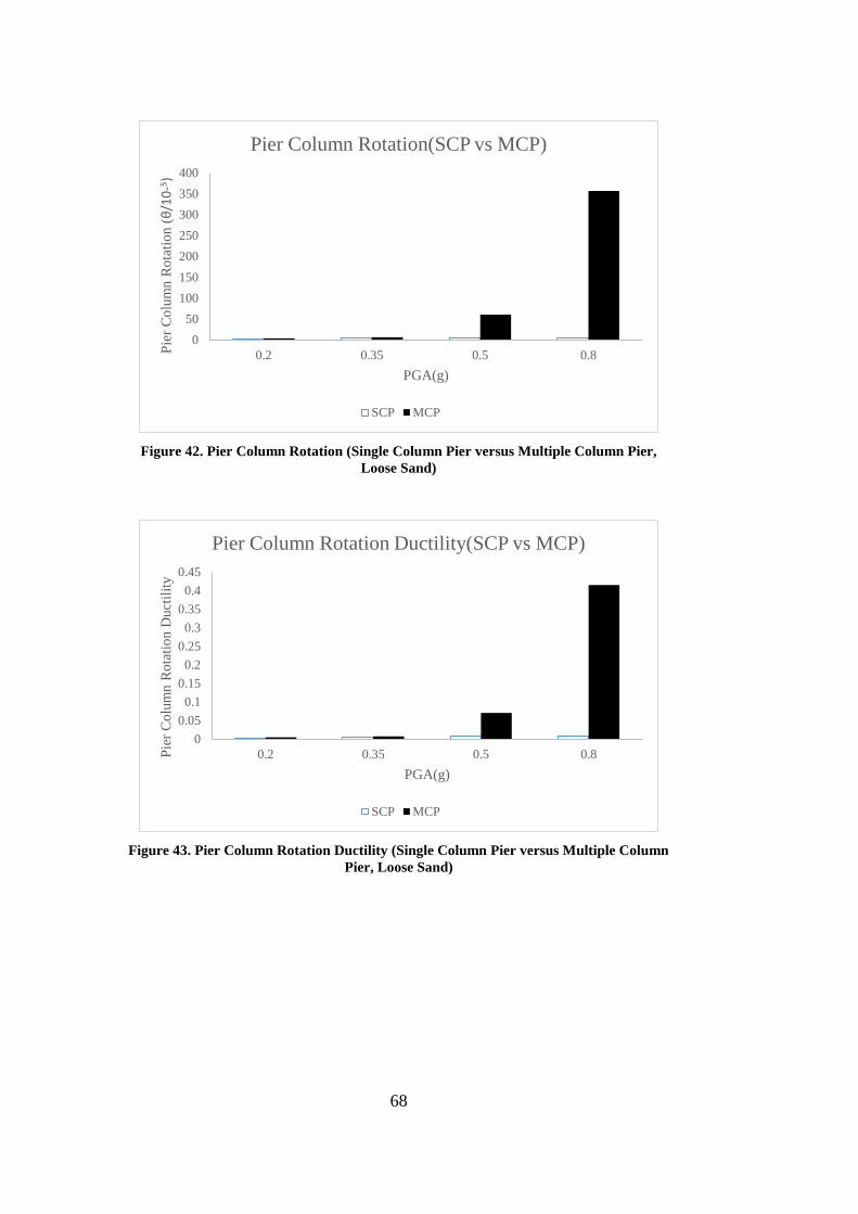
68

Figure 42. Pier Column Rotation (Single Column Pier versus Multiple Column Pier,

Loose Sand)

Figure 43. Pier Column Rotation Ductility (Single Column Pier versus Multiple Column

Pier, Loose Sand)

0

50

100

150

200

250

300

350

400

0.2 0.35 0.5 0.8Pie

r C

olu

mn R

ota

tio

n (θ

/10

-5 )

PGA(g)

Pier Column Rotation(SCP vs MCP)

SCP MCP

0

0.05

0.1

0.15

0.2

0.25

0.3

0.35

0.4

0.45

0.2 0.35 0.5 0.8Pie

r C

olu

mn R

ota

tio

n D

uct

ilit

y

PGA(g)

Pier Column Rotation Ductility(SCP vs MCP)

SCP MCP

69

Figure 44. Footing Vertical Displacement (Single Column Pier versus Multiple Column

Pier, Loose Sand)

Figure 45. Footing Rotation (Single Column Pier versus Multiple Column Pier, Loose Sand

0

0.005

0.01

0.015

0.02

0.025

0.2 0.35 0.5 0.8Ab

utm

ent

Dis

pla

cem

ent

(mm

)

PGA(g)

Footing Vertical Displacement(SCP vs MCP)

SCP MCP

0

0.0002

0.0004

0.0006

0.0008

0.001

0.0012

0.0014

0.0016

0.0018

0.2 0.35 0.5 0.8

Fo

oti

ng R

ota

tio

n

PGA(g)

Footing Rotation(SCP vs MCP)

SCP MCP

70

Figure 46. Footing Sliding Displacement (Single Column Pier versus Multiple Column

Pier, Loose Sand)

According to Figure 33, deck displacement significantly increases under 0.8g

peak ground acceleration. Under every peak ground acceleration given to the

bridges, multi-column pier bent always shows more drift compared to

hammerhead pier. In Figure 35, it is obvious that multiple column pier bent

rotates more than single column pier. In Figure 36, the ductility level cannot be

reached at any peak ground acceleration since under the the characteristic

compressive strength of C25 concrete and yield strength of steel are input to the

system as 32.48 MPa and 503 MPa because according to the article of Yücemen

and Fırat (2014), the average values come as 32.48 MPa and 503 MPa,

respectively. Furthermore, the bridge considered in this study is designed for

0.35g peak ground acceleration. Hence, the resistance of the bridges rises up to

0.5g. Moreover, in every analysis under 1.5g peak ground acceleration, soil

yielded. Hence, the pier cannot yield because the soil yielded first. Figures 37

and 38 show that footing shows more displacement in the analyses conducted by

single column pier. In Figure 39, footing shows large displacement when the

peak ground acceleration reaches 0.8g.

0

0.05

0.1

0.15

0.2

0.25

0.3

0.35

0.4

0.45

0.5

0.2 0.35 0.5 0.8

Fo

oti

ng S

lid

ing D

isp

.(m

m)

PGA(g)

Footing Sliding Displacement(SCP vs MCP)

SCP MCP

71

CHAPTER 8

8. CONCLUSION

In this thesis, comparative seismic performance assessment of continuous slab

on girder bridges with multi column pier bent and hammerhead pier for soft and

stiff soil conditions is studied. Based on this study, the soil-structure interaction

is taken into account in order to model the structure realistically. 112 analyses

are conducted under medium and loose conditions of soil in transverse direction

and conclusion is drawn as follows:

Despite the fact that the piers are designed for 0.35 g in real life, majority of the

piers did not yield under seismic excitation. This might occur since the mean

yield strength of steel is taken as 503 MPa and the characteristic compressive

strength of C25 concrete, is taken as 32.48 MPa. These two parameters might

increase the yield point.

Furthermore the springs used in the model, might have absorbed the energy

which comes due to seismic excitation.

Last but not least, the frictional pendulums on the abutments, play a significant

role on reducing the energy due to seismic excitation.

The results of the analyses show that, under medium dense sand conditions,

multiple column piers rotate more than hammerhead piers and footing vertical

displacement of multiple column is higher than the footing vertical displacement

of hammerhead.

73

REFERENCES

1. AASHTO LRFD Bridge Design Specifications. (2014). Washington.

2. Anastasopoulos, I., Gelagoti, F., Kourkoulis, R., & Gazetas, G. (2011).

Simplified Constitutive Model for Simulation of Cyclic Response of Shallow

Foundations: Validation against Laboratory Tests. Journal of Geotechnical

and Geoenvironmental Engineering, 137(12), 1154-1168.

doi:10.1061/(asce)gt.1943-5606.0000534

3. Anastasopoulos, I., Kourkoulis, R., Gelagoti, F., & Papadopoulos, E. (2012).

Rocking response of SDOF systems on shallow improved sand: An

experimental study. Soil Dynamics and Earthquake Engineering, 40, 15-33.

doi:10.1016/j.soildyn.2012.04.006

4. Deng, L., Kutter, B. L., & Kunnath, S. K. (2012). Centrifuge Modeling of

Bridge Systems Designed for Rocking Foundations. Journal of Geotechnical

and Geoenvironmental Engineering, 138(3), 335-344.

doi:10.1061/(asce)gt.1943-5606.0000605

5. Gajan, S., & Kutter, B. L. (2008). Effect of Critical Contact Area Ratio on

Moment Capacity of Rocking Shallow Footings. Geotechnical Earthquake

Engineering and Soil Dynamics IV. doi:10.1061/40975(318)133

6. Gajan, S., & Kutter, B. L. (2009). Contact Interface Model for Shallow

Foundations Subjected to Combined Cyclic Loading. Journal of

Geotechnical and Geoenvironmental Engineering,135(3), 407-419.

doi:10.1061/(asce)1090-0241(2009)135:3(407)

7. Gajan, S., & Kutter, B. L. (2009). Effects of Moment-to-Shear Ratio on

Combined Cyclic Load-Displacement Behavior of Shallow Foundations

74

from Centrifuge Experiments. Journal of Geotechnical and

Geoenvironmental Engineering, 135(8), 1044-1055.

8. Gajan, S., Hutchinson, T., Kutter, B., Raychowdhury, P., Ugalde, J., &

Stewart, J. (2008). Numerical models for analysis and performance-based

design of shallow foundations subjected to seismic loading. Berkeley, CA:

Pacific Earthquake Engineering Research Center.

9. Gajan, S., Kutter, B. L., Phalen, J. D., Hutchinson, T. C., & Martin, G. R.

(2005). Centrifuge modeling of load-deformation behavior of rocking

shallow foundations. Soil Dynamics and Earthquake Engineering,25(7-10),

773-783. doi:10.1016/j.soildyn.2004.11.019

10. Gajan, S., Kutter, B. L., Phalen, J. D., Hutchinson, T. C., & Martin, G. R.

(2005). Centrifuge modeling of load-deformation behavior of rocking

shallow foundations. Soil Dynamics and Earthquake Engineering, 25(7-10),

773-783. doi:10.1016/j.soildyn.2004.11.019

11. Gajan, S., Kutter, B., & Thomas, J. (2005). Physical and numerical modeling

of cyclic moment-rotation behavior of shallow foundations.

12. Harden, C. W., Hutchinson, T., Martin, G. R., and Kutter, B. L., 2005,

Numerical modeling of the nonlinear cyclic response of shallow foundations,

Report No. PEER‐ 2005/04, Pacific Earthquake Engineering Research

Center, University of California, Berkeley.

13. Kausel, E. (2010). Early history of soil–structure interaction. Soil Dynamics

and Earthquake Engineering, 30(9), 822-832.

doi:10.1016/j.soildyn.2009.11.001

14. Kim, Y., & Roesset, J. M. (2004). Effect of Nonlinear Soil Behavior on

Inelastic Seismic Response of a Structure. International Journal of

Geomechanics, 4(2), 104-114. doi:10.1061/(asce)1532-3641(2004)4:2(104)

75

15. Kokkali, P., Abdoun, T., & Anastasopoulos, I. (2015). Centrifuge Modeling

of Rocking Foundations on Improved Soil. Journal of Geotechnical and

Geoenvironmental Engineering,141(10), 04015041.

doi:10.1061/(asce)gt.1943-5606.0001315

16. Mylonakis, G., Nikolaou, S., & Gazetas, G. (2006). Footings under seismic

loading: Analysis and design issues with emphasis on bridge

foundations. Soil Dynamics and Earthquake Engineering, 26(9), 824-853.

doi:10.1016/j.soildyn.2005.12.005

17. Negro, P., Paolucci, R., Pedretti, S., & Faccioli, E. (2000). Large-scale soil-

structure interaction experiments on sand under cyclic loading.

18. Raychowdhury, P., & Hutchinson, T. (2008). Nonlinear Material Models for

Winkler-Based Shallow Foundation Response Evaluation. GeoCongress

2008. doi:10.1061/40972(311)85

19. Saadeghvaziri, M., Yazdani-Motlagh, A., & Rashidi, S. (2000). Effects of

soil–structure interaction on longitudinal seismic response of MSSS

bridges. Soil Dynamics and Earthquake Engineering, 20(1-4), 231-242.

doi:10.1016/s0267-7261(00)00056-7

20. Salgado, R. (2003). The Engineering of Foundations.

21. Seismic Design of Highway Bridge Foundations (Vol. 2). (1986). McLean,

Virginia: US Department of Transportation.

22. Shirato, M., Kouno, T., Asai, R., Nakatani, S., Fukui, J., & Paolucci, R.

(2008). Large-Scale Experiments On Nonlinear Behavior Of Shallow

Foundations Subjected To Strong Earthquakes. Soils And

Foundations, 48(5), 673-692. doi:10.3208/sandf.48.673

23. Shirato, M., Yoshinori, N., & Ryuichi, A. (2005). Experimental study on the

residual displacement of shallow foundations subjected to cyclic loads.

76

24. Ugalde, J., Kutter, B., Jeremic, B., & Gajan, S. (2007). Centrifuge modelling

of rocking behavior of bridges on shallow foundations.

25. Yücemen, S., & Fırat, F. K. (2014). Determination of New Load and

Resistance Factors for Reinforced Concrete Structural Members.