
COMPARATIVE REVIEW OF POSSIBLE ALTERNATIVES FOR …
97
COMPARATIVE REVIEW OF POSSIBLE ALTERNATIVES FOR PERFORMING SAFETY ASSESSMENT OF DESIGN RULES FOR STEEL STRUCTURES FCTUC 2014 Trayana Tankova COMPARATIVE REVIEW OF POSSIBLE ALTERNATIVES FOR PERFORMING SAFETY ASSESSMENT OF DESIGN RULES FOR STEEL STRUCTURES Trayana Tankova Supervisors: Professor Luís Alberto Proença Simões da Silva Drª Liliana Marques University of Coimbra 06.01.2014 Thesis Submitted in partial fulfillment of requirements for the degree of Master of Science in Construction of Steel and Composite Structures European Erasmus Mundus Master Sustainable Constructions under natural hazards and catastrophic events
Transcript of COMPARATIVE REVIEW OF POSSIBLE ALTERNATIVES FOR …

CO
MPA
RATI
VE R
EVIE
W O
F PO
SSIB
LE A
LTER
NA
TIVE
S FO
R PE
RFO
RMIN
G S
AFE
TY A
SSES
SMEN
T O
F D
ESIG
N R
ULE
S FO
R ST
EEL
STRU
CTU
RES
FCTU
C20
14Tr
ayan
aTa
nkov
a
COMPARATIVE REVIEW OF POSSIBLE ALTERNATIVES FORPERFORMING SAFETY ASSESSMENT OF DESIGN RULES FOR
STEEL STRUCTURES
Trayana Tankova
Supervisors: Professor Luís Alberto Proença Simões da Silva
Drª Liliana Marques
University of Coimbra
06.01.2014
Thesis Submitted in partial fulfillment of requirements for the degree of Master ofScience in Construction of Steel and Composite Structures European Erasmus Mundus Master Sustainable Constructions under natural hazards and catastrophic events

COMPARATIVE REVIEW OF POSSIBLE ALTERNATIVES FOR
PERFORMING SAFETY ASSESSMENT OF DESIGN RULES FOR
STEEL STRUCTURES
AUTHOR
TRAYANA TANKOVA
SUPERVISOR PROF. LUÍS SIMÕES DA SILVA
CO-SUPERVISOR DR. LILIANA MARQUES
UNIVERSITY UNIVERSIDADE DE COIMBRA
DATE 06/01/2014, COIMBRA


European Erasmus Mundus Master
Sustainable Constructions under natural hazards and
catastrophic events
520121‐1‐2011‐1‐CZ‐ERA MUNDUS‐EMMC
Trayana Tankova i
ACKNOWLEDGEMENTS
During this master programme many people supported me and I am very grateful to them.
This thesis would not be possible without the major contribution of my supervisor – Prof. Luís Simões
da Silva. I am very grateful to him for his patience, constructive judgment and support during the
period of study, moreover for the opportunity to work with his team at the University of Coimbra. In
addition, I am thankful for everything he did for my colleagues from the SUSCOS_M master course
and me during the first semester in Coimbra.
Furthermore, I would like to express my sincere gratitude to my co-supervisor - Dr. Liliana Marques.
I am very glad that I had the chance to collaborate with her. She was very supportive in difficult
moments and she always provided me with creative ideas which were valuable for my work.
A great appreciation to the European Commission for the financial support during my studies in the
Erasmus Mundus Programme SUSCOS_M, without their support this degree would be very difficult.
Moreover, I would like to thank them for the wonderful idea of Erasmus Mundus, it is truly a lifetime
experience, not only in terms of education but also as life lessons.
Life is not only at the university and everybody needs their true friends. I am very thankful to my
friends and I appreciate their ability to cheer me up in hard times and to celebrate my happiness.
Even though we do not spend as much time as we did years ago, they will always be in my heart and
mind.
During this master course, all SUSCOS_M students became attached to each other, even we used to
say that we are the “Suscos family”. This expression is more than true and brilliantly describes our
relationship. I am glad we experienced this year together and I think everyone made the others better
by sharing their own culture. I could not be happier I met all of them.
At least but not the last, I would like to thank to my mother, father and brother. There are no words
which can express my gratitude to them. They gave me the opportunity to be the person I am now and
they have always been supportive to all of my adventures. To them I dedicate this thesis.


European Erasmus Mundus Master
Sustainable Constructions under natural hazards and
catastrophic events
520121‐1‐2011‐1‐CZ‐ERA MUNDUS‐EMMC
Trayana Tankova iii
ABSTRACT
Currently, safety assessment is not consistently considered throughout Eurocode 3, mainly due to lack
of guidance and existing databanks containing information on distribution of relevant basic variables
and steel properties. In addition, some rules are not thoroughly validated, leading to higher
uncertainties.
In establishing the partial safety factor - γM of a design procedure, scatter related to material and
geometrical properties may be isolated from resistance model. Simplified safety assessment
procedures are analysed and further tested in which the basic variables are assumed independent from
each other, with basis on EN 1990 safety assessment procedure.
In this dissertation, firstly, a theoretical overview is proposed in order to introduce the basic principles
in the probability theory; secondly, the basic principles of design codes are presented, focusing on the
current European design codes EN 1990 to EN 1999. The design methodologies are listed and their
background is discussed, and furthermore focus is given to the procedures applicable to Eurocode 3.
The safety assessment procedure, given in Annex D of EN 1990 is also presented and its theoretical
background is clarified.
Subsequently, an analytical review of existing methodologies for safety assessment of design rules for
steel structures is carried out. The procedures are presented and their field of application is detailed.
Furthermore, numerical validation of simplified procedures, based on assumed distributions of basic
variables such as material and cross-section properties, is performed focusing on stability failure
modes, in particular flexural buckling of columns.
In addition, a numerical example is presented, which aims at further clarifying latter methodologies.
Sensitivity analysis is performed in order to assess the influence of different basic variables. In this
example, statistical distributions of the imperfections are also considered.
Finally, the statistical dependence of basic variables is discussed, based on correlation between yield
stress and plate thickness. In order to obtain a reasonable correlation coefficient, statistical data from
real experiments is used.
This dissertation is part of European research project SAFEBRICTILE RFS-PR-12103 – SEP nº
601596, where safety assessment procedure is developed for brittle to ductile failure modes.
Therefore, it is considered a valuable contribution for achieving the project goals and further
improvement of the design methodologies in the Eurocodes.


European Erasmus Mundus Master
Sustainable Constructions under natural hazards and
catastrophic events
520121‐1‐2011‐1‐CZ‐ERA MUNDUS‐EMMC
Trayana Tankova v
TABLE OF CONTENTS
ACKNOWLEDGEMENTS ................................................................................................................................. I
ABSTRACT ....................................................................................................................................................... III
TABLE OF CONTENTS .................................................................................................................................... V
NOTATIONS .................................................................................................................................................... VII
1 INTRODUCTION ....................................................................................................................................... 1
2 THEORETICAL OVERVIEW .................................................................................................................. 3
2.1 UNCERTAINTY IN ENGINEERING ............................................................................................................. 3 2.2 FUNDAMENTALS OF PROBABILITY THEORY ............................................................................................ 4 2.3 PROBABILITY MODELS ........................................................................................................................... 5 2.4 PROBABILITY DISTRIBUTIONS ................................................................................................................ 8
2.4.1 The Gaussian (Normal) Distribution ................................................................................................ 8 2.4.2 The Lognormal Distribution ............................................................................................................. 9
2.5 INTRODUCTION TO STATISTICS ............................................................................................................. 10 2.6 COVARIANCE AND CORRELATION ........................................................................................................ 11 2.7 MOMENTS OF FUNCTIONS OF RANDOM VARIABLES .............................................................................. 12 2.8 REGRESSION ANALYSIS ........................................................................................................................ 13
3 BASIS OF DESIGN ................................................................................................................................... 17
3.1 GENERAL OVERVIEW OF EN 1990 ........................................................................................................ 17 3.2 METHODOLOGICAL ASSUMPTIONS FOR DESIGN RESISTANCE ................................................................ 20
3.2.1 Design resistance ............................................................................................................................ 20 3.2.2 Partial factors in EN 1990 .............................................................................................................. 21
3.3 SAFETY ASSESSMENT PROCEDURE – ANNEX D DESIGN ASSISTED BY TESTING ..................................... 22 3.3.1 Error related to the design model ................................................................................................... 23 3.3.2 Error related to the basic input variables ....................................................................................... 24 3.3.3 The partial safety factor .................................................................................................................. 26
4 ALTERNATIVES FOR SAFETY ASSESSMENT ................................................................................. 31
4.1 ASSUMPTIONS ...................................................................................................................................... 31 4.2 PROCEDURE 0 (P0) ............................................................................................................................... 33 4.3 PROCEDURE 1 (P1) ............................................................................................................................... 34
4.3.1 Description ..................................................................................................................................... 34 4.3.2 Assessment of the conservative nature of Procedure 1 ................................................................... 35
4.4 PROCEDURE 2 (P2) ............................................................................................................................... 40 4.5 SUMMARY ............................................................................................................................................ 42
5 NUMERICAL VALIDATION OF POSSIBLE ALTERNATIVES ...................................................... 45
5.1 INTRODUCTION .................................................................................................................................... 45 5.2 GENERATION OF SAMPLES.................................................................................................................... 46
5.2.1 Yield strength .................................................................................................................................. 46

European Erasmus Mundus Master
Sustainable Constructions under natural hazards and
catastrophic events
520121‐1‐2011‐1‐CZ‐ERA MUNDUS‐EMMC
vi Trayana Tankova
5.2.2 Geometrical properties ................................................................................................................... 48 5.2.3 Modulus of elasticity ....................................................................................................................... 49
5.3 RESULTS .............................................................................................................................................. 50 5.3.1 Methodology ................................................................................................................................... 50 5.3.2 Numerical assessment of P1 ........................................................................................................... 51 5.3.3 Numerical assessment of P2 ........................................................................................................... 55
6 NUMERICAL EXAMPLE ....................................................................................................................... 59
6.1 DEFINITION AND PURPOSE .................................................................................................................... 59 6.1.1 Cases ............................................................................................................................................... 60 6.1.2 Samples ........................................................................................................................................... 60
6.2 NUMERICAL MODELLING [17] .............................................................................................................. 63 6.3 RESULTS AND DISCUSSION ................................................................................................................... 65
6.3.1 Introduction .................................................................................................................................... 65 6.3.2 Influence of each basic variable ..................................................................................................... 65 6.3.3 Combinations of basic variables ..................................................................................................... 67 6.3.4 Influence of modelling with nominal parameters............................................................................ 69 6.3.5 Influence of geometrical parameters .............................................................................................. 72 6.3.6 Simplified procedures ..................................................................................................................... 73
7 BRIEF ANALYSIS OF THE STATISTICAL DEPENDENCY BETWEEN BASIC VARIABLES .. 77
7.1 CORRELATION BASED ON EXPERIMENTS .............................................................................................. 77 7.2 IMPLEMENTATION OF THE CORRELATION ............................................................................................. 78
8 CONCLUSIONS ........................................................................................................................................ 81
REFERENCES ................................................................................................................................................... 83

European Erasmus Mundus Master
Sustainable Constructions under natural hazards and
catastrophic events
520121‐1‐2011‐1‐CZ‐ERA MUNDUS‐EMMC
Trayana Tankova vii
NOTATIONS
Latin upper case letters
Cov(.) Covariance
E(.) Mean value
E Event
Ed Design value of the actions
FX Cumulative distribution function for the random variable X
P(.) Probability
Pf Probability of failure
Rd Design value of the resistance
S Certain event
Var(.) Variance
VX Coefficient of variation
Vδ Estimator for the coefficient of variation of the error term
X Random variable
mX Array of mean values of basic variables
nomX Array of nominal values of basic variables
Latin lower case letters
b Correction factor
fX(x) Probability density function for the random variable X
)(Xgrt Resistance function used as a design model
ndk , Design fractile factor
n Number of experiments or numerical results
dr Design value of the resistance

European Erasmus Mundus Master
Sustainable Constructions under natural hazards and
catastrophic events
520121‐1‐2011‐1‐CZ‐ERA MUNDUS‐EMMC
viii Trayana Tankova
er Experimental resistance value
nr Nominal value of the resistance
tr Theoretical resistance determined with )(Xgrt
s Estimated value for the standard deviation σ
sΔ Estimated value for the standard deviation σΔ
x Estimated value for the mean value
Greek upper case letters
Δ Logarithm of the error term δ
Estimated value for E(Δ)
Φ cumulative distribution function (CDF) for the standard normal distribution
Greek lower case letters
αE FORM (First Order Reliability Method) sensitivity factor for effects of actions
αR FORM (First Order Reliability Method) sensitivity factor for resistance
β reliability index
F Partial factor for actions, also accounting for model uncertainties and dimensional
variations
f Partial factor for actions, which takes account of the possibility of unfavorable
deviations of the action values from the representative values
M Partial safety factor for a material property also accounting for model uncertainties
and model variations
*M Corrected partial safety factor for resistances
m Partial factor for a material property
European Erasmus Mundus Master
Sustainable Constructions under natural hazards and
catastrophic events
520121‐1‐2011‐1‐CZ‐ERA MUNDUS‐EMMC
Trayana Tankova ix
Rd Partial factor associated with the uncertainty of the resistance model
Sd Partial factor associated with the uncertainty of the action and/or action effect model
δ Error term
δi Observed error term for test specimen i
δx Coefficient of variation of the random variable X
λ Mean value of lnX
μx Mean value of the random variable X
ρ Correlation coefficient
ξ Standard deviation of lnX
σ Standard deviation
σΔ2 Variance of the term Δ
σX Standard deviation of the random variable X


European Erasmus Mundus Master
Sustainable Constructions under natural hazards and
catastrophic events
520121‐1‐2011‐1‐CZ‐ERA MUNDUS‐EMMC
Trayana Tankova 1
1 INTRODUCTION
In real world engineering problems, uncertainties are unavoidable. This issue fully applies to
structural engineering. Engineers face problems concerning deviations from their models as well as
deviations from the material and geometrical properties on an everyday basis. In this sense, it is
important to recognize those problems and to deal with them in an efficient manner. For many years, a
way to deal with this problem is using design codes, which incorporate the scatter due to randomness
of reality.
In this thesis, it is aimed to compare various methodologies for the safety assessment of stability
design rules and the corresponding safety factor γM on the basis of EN 1990 [1] and its Annex D. The
main objective of this comparison is to support the preparation of clear and unambiguous guidance for
the development and assessment of design rules in Eurocode 3 [2].
The structure of this work is the following:
Firstly, a brief theoretical overview is presented, in order to introduce the reader to the
theoretical background of the subject;
Secondly, an overview of the basis of structural design according to the Eurocodes is
presented;
Subsequently, simplifications for safety assessment of design rules are explained – the
methods are briefly summarized and differences between them are emphasized;
Consequently, a numerical assessment of the possible alternatives is performed and
further discussed based on flexural buckling of columns;
Furthermore, an example is provided in order to illustrate the application of the various
alternatives;
Finally, an attempt to consider statistical dependence between basic variables is
provided, focusing on correlation between yield stress and plate thickness;


European Erasmus Mundus Master
Sustainable Constructions under natural hazards and
catastrophic events
520121‐1‐2011‐1‐CZ‐ERA MUNDUS‐EMMC
Trayana Tankova 3
2 THEORETICAL OVERVIEW
The safety assessment is performed due to the randomness of the relevant basic variables. Therefore,
in this section, it is intended to briefly clarify the theoretical background of probability and statistical
concepts (as proposed in [3]). The following main topics are included:
Uncertainties;
Fundamentals of probability theory;
Probability distributions;
Introduction to statistics;
Covariance and correlation;
Moments of functions of random variables;
Regression analysis;
2.1 UNCERTAINTY IN ENGINEERING
Uncertainties are existing in engineering problems and are clearly unavoidable. The available data is
often incomplete or insufficient and inevitably contains variability. Moreover, the design
methodologies used to estimate and/or predict reality lie on certain assumptions and simplifications,
and therefore introduce additional uncertainty. In practice, two broad types of uncertainties are
recognized: i) aleatory uncertainty associated with the randomness of the underlying phenomenon that
is demonstrated as variability in the observed information; ii) epistemic uncertainty associated with
the imperfect models of the real world due to insufficient or imperfect knowledge of the reality;
Many phenomena which are of engineering focus contain randomness, in a sense that measurements
or experiments differ one from each other even though they are performed in identical conditions. In
other words, there is a range of occurrence, and even certain values may occur more frequently than
others. The variability characteristics in such data or information have a statistical nature. For
example, aleatory uncertainty can be the variability of the yield stress in steel, deviations of the
geometrical properties, etc. Steel profiles are produced in the same conditions; the tests are performed
using the same test set up, usually standardized; however, not always the same measure is found, but
rather a range of measurements. This problem is of particular interest in this thesis. Another example
can be the compression strength of concrete which is highly variable. The parameters which influence
the production of concrete are many and some of them are hard to control. Therefore, the resulting
strength can be found with a high coefficient of variation.
As already mentioned, the other main type of uncertainty is associated with the imperfect knowledge
or the so-called epistemic uncertainty. In engineering problems, the solutions always rely on idealized
models of the real world. These models –mathematical, laboratory, numerical etc. – are imperfect
representations of the real problem. They are inaccurate with some unknown degree of error and thus
are imposing uncertainty. This uncertainty sometimes can be more significant than the aleatory
uncertainty. An example of epistemic uncertainty is every design rule that is written in the design

European Erasmus Mundus Master
Sustainable Constructions under natural hazards and
catastrophic events
520121‐1‐2011‐1‐CZ‐ERA MUNDUS‐EMMC
4 Trayana Tankova
code. Design rules have uncertainties incorporated, although these rules are calibrated in a way that
the variability of this uncertainty aims to be always safe-sided.
An efficient way to deal with uncertainties is given by the probability theory and statistics. They can
be used effectively to “quantify” the uncertainty and therefore to provide aid in decision making
process. In the following sections, the essentials of probability theory are briefly summarized.
2.2 FUNDAMENTALS OF PROBABILITY THEORY
The probability can be considered as a numerical measure of the likelihood of occurrence of an event
within a set of all possible alternative events. Therefore, an event can be identified as a main unit in
the formulation. Subsequently, the first requirement in the formulation of the probabilistic problem is
the identification of the set of all possibilities i.e. the probability space for the event of interest.
Probabilities are always associated with specific events within certain probability space and they are
only valid for that specific probability space. Hence, each probability space can contain many events,
and each event has certain probability of occurrence in that probability space.
In order to formulate the probabilistic problem, elementary set theory is used. Following the set
theory, the set of all probabilities in a probabilistic problem is collectively defined as a sample space,
and each of the individual possibilities is a sample point. An event is recognized as a subset of the
sample space.
The sample spaces can be discrete or continuous, as the discrete space can be finite or infinite. The
following special events are recognized within the sample spaces:
Impossible event – φ, it is an even with no sample point. This event can be also referred as an
empty set;
Certain event – S, it is the event containing all sample points in the sample space, therefore
the certain event is the space itself;
Complementary event E , of the event E which contains all sample points which are not in E;
The concept is further clarified by Figure 2.1, in which the so-called Venn diagram is used to
illustrate the sample space S and its events. Moreover, the union or intersection of events may be of
interest, as shown in Figure 2.2. Those operations are similar to sum and multiplication of numbers,
however they are not of special interest here and they will not be further discussed.
Figure 2.1Venn diagram of sample space S

European Erasmus Mundus Master
Sustainable Constructions under natural hazards and
catastrophic events
520121‐1‐2011‐1‐CZ‐ERA MUNDUS‐EMMC
Trayana Tankova 5
Figure 2.2Examples of union and intersection events
Another type of events is the mutually exclusive events, those are events which cannot occur
simultaneously and their corresponding subsets do not have intersections. An example of mutually
exclusive events is the steel stress being above and below the yield strength at the same time. The
mutually exclusive event should not be confused for statistically independent events. The statistically
independent events are those whose occurrence does not exclude the occurrence of the other. They
might exist simultaneously; however, there is no dependence, on the contrary in case of mutually
exclusive events, the occurrence of both is impossible.
As any other mathematical model, the theory of probability is based on few axioms. The axioms of
the probability theory are:
Axiom 1: for every event E in a sample space S, there is a probability:
0)( EP (2.1)
Axiom 2: the probability of the certain event S is:
0.1)( SP (2.2)
Axiom 3: for two events E1 and E2 which are mutually exclusive, the following can be
written:
)()()( 2121 EPEPEEP (2.3)
2.3 PROBABILITY MODELS
When dealing with probabilities, the basic variables are defined as a range of possible values, unlike
the deterministic problems where the variables are associated with actual values. Therefore, when
using probabilities the random variables are defined as upper case letters. If X is a random variable
then X=x, X>x or X<x represent different events, where x belonging to (a;b) is the mapping of the
event. In Figure 2.3 the concept of mapping is defined, as the sample space was previously clarified
when dealing with sets. In order to apply the probability concepts, it is more convenient to use
intervals rather than the sets as explained in the previous section.

European Erasmus Mundus Master
Sustainable Constructions under natural hazards and
catastrophic events
520121‐1‐2011‐1‐CZ‐ERA MUNDUS‐EMMC
6 Trayana Tankova
An example of two defined events is presented on Figure 2.3:
bXaE 1
dXcE 2
And their intersection is found as:
bXcEE 21
Figure 2.3Mapping through X
The random variables, previously defined, are associated with probability measures called probability
distributions or “probability law”. For each random variable, its probability distribution can always be
described by its cumulative distribution function (CDF):
xxXPFX )( (2.4)
In case that X is a discrete random variable, its probability distribution is described by probability
mass function (PMF), where the CDF can be found as:
xx
iXxx
iX
ii
xpxXPF )()( (2.5)
On the contrary, if X is continuous, it is defined in an interval, therefore for specific value X=x, only
the probability density can be obtained, there is no probability. Hence, for continuous random
variables the probability law is described by the probability density function, which is denoted as fX(x)
such that:

European Erasmus Mundus Master
Sustainable Constructions under natural hazards and
catastrophic events
520121‐1‐2011‐1‐CZ‐ERA MUNDUS‐EMMC
Trayana Tankova 7
b
a
XX xFdxxfbXaP )()( (2.6)
a
X
b
X dxxfdxxfbXaP )()( (2.7)
Every function used to describe the probability distribution of a random variable should satisfy the
axioms of the probability theory previously listed, in a way that:
0)( XF and 0.1)( XF
0)( xFX for all x;
)(xFX is continuous with x;
Any random variable in practice can be fully described by its probability distribution and each needed
parameter can be obtained from the CDF, although in reality it is often difficult to know the exact
distribution of a variable. Therefore, assumptions on the distribution can be made based on its main
descriptors.
The random variable is associated with a range of values, thus a central value would be of specific
interest. Such value is the so-called mean value which represents the weighted average of the random
variable (it is defined as weighted average, since for x of X there is an associated probability). The
mean value is often denoted with E(X) and it can also be referred as expected value. It can be found
from the following expressions:
XX dxxxfXE
)()( (2.8)
Xx
iXi
i
xpxXE
)()( (2.9)
Another very useful parameter is the degree of the dispersion of the random variable. It is of special
interest, since it shows how close/far from the mean value are all the values spreading. Therefore, this
descriptor should be defined as a function of the mean value. This measure is known as the variance
of the distribution or the second central moment. It can be found using the following expressions for
the continuous and discrete variable respectively:
dxxfxXVar XX )()()( 2 (2.10)
ix
iXiX xpxxXVar )()()( 2 (2.11)
European Erasmus Mundus Master
Sustainable Constructions under natural hazards and
catastrophic events
520121‐1‐2011‐1‐CZ‐ERA MUNDUS‐EMMC
8 Trayana Tankova
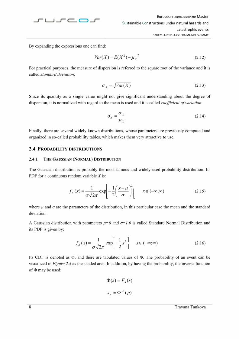
By expanding the expressions one can find:
22 )()( XXEXVar (2.12)
For practical purposes, the measure of dispersion is referred to the square root of the variance and it is
called standard deviation:
)(XVarX (2.13)
Since its quantity as a single value might not give significant understanding about the degree of
dispersion, it is normalized with regard to the mean is used and it is called coefficient of variation:
X
XX
(2.14)
Finally, there are several widely known distributions, whose parameters are previously computed and
organized in so-called probability tables, which makes them very attractive to use.
2.4 PROBABILITY DISTRIBUTIONS
2.4.1 THE GAUSSIAN (NORMAL) DISTRIBUTION
The Gaussian distribution is probably the most famous and widely used probability distribution. Its
PDF for a continuous random variable X is:
);(2
1exp
2
1)(
2
xx
xf X
(2.15)
where µ and σ are the parameters of the distribution, in this particular case the mean and the standard
deviation.
A Gaussian distribution with parameters µ=0 and σ=1.0 is called Standard Normal Distribution and
its PDF is given by:
);(2
1exp
2
1)( 2
xxxf X
(2.16)
Its CDF is denoted as Φ, and there are tabulated values of Φ. The probability of an event can be
visualized in Figure 2.4 as the shaded area. In addition, by having the probability, the inverse function
of Φ may be used:
)()( sFs S
)(1 ps p

European Erasmus Mundus Master
Sustainable Constructions under natural hazards and
catastrophic events
520121‐1‐2011‐1‐CZ‐ERA MUNDUS‐EMMC
Trayana Tankova 9
Figure 2.4 The Standard Normal Distribution
Moreover, due to the symmetry of the PDF of the standard normal distribution about zero, then the
following can be written:
)(1)( ss
A convenient way to use the CDF of the standard normal distribution can be derived from Eq.2.7. The
probability can then be found using the expression:
ab
bXaP (2.17)
2.4.2 THE LOGNORMAL DISTRIBUTION
The lognormal distribution is also a very popular probability distribution. The PDF of the lognormal
distribution can be found as:
);0[ln
2
1exp
2
1)(
2
x
x
xxf X
(2.18)
The parameters of the distribution are λ and ξ, which are respectively the mean and standard deviation
of lnX. It can be easily proven that for a random variable X with a lognormal distribution and
parameters of the distribution λ and ξ, then lnX is normal with mean λ and standard deviation ξ, i.e.
N(λ ,ξ). This is a valuable feature which can be used similarly to Eq.(2.17):
ab
bXaPlnln
(2.19)
It was seen that both distributions can be connected, and therefore the transformation expressions can
be derived from the normal to lognormal parameters and vice-versa, using:
2
2
1ln X (2.20)

European Erasmus Mundus Master
Sustainable Constructions under natural hazards and
catastrophic events
520121‐1‐2011‐1‐CZ‐ERA MUNDUS‐EMMC
10 Trayana Tankova
2
2
2 1ln1ln XX
X
(2.21)
2.5 INTRODUCTION TO STATISTICS
In the previous sections, the probability theory was summarized. In the real life, however, distribution
of variables is based on observation of data, i.e. the theoretical distributions are chosen in a way to fit
the real behaviour. Moreover, the observed data is usually a test sample or many test samples which
are part of the population of the observed parameter, and therefore, additional error due to the limited
information should be avoided. The statistics constitutes methods to link the real observations with
probability theory. Those principles are based on estimates of the real parameters of the distribution.
There are different methods for estimating the parameters, however they all should satisfy certain
requirements:
Unbiasedness – if repeated estimations of the parameter are performed and their mean is
equal to the parameter, then the estimator is called unbiased;
Consistency – if the sample size approaches infinity, then the estimator tends to the value of
the parameter;
Efficiency – one estimator is more efficient than the other, if the variance of the first is
smaller than the second;
Sufficiency – an estimator is considered sufficient, if it can capture all the information in a
sample that is relevant for the estimation of the parameter;
Figure 2.5 Statistics
In reality, however, it is hardly possible to satisfy all of the above parameters of an estimator. Usually,
the properties are chosen with respect to the specific needs for estimation.
Previously, it was presented that the mean and standard deviation of a distribution are of specific
interest and hereby, the unbiased estimators for the sample mean and the sample variance are
presented:

European Erasmus Mundus Master
Sustainable Constructions under natural hazards and
catastrophic events
520121‐1‐2011‐1‐CZ‐ERA MUNDUS‐EMMC
Trayana Tankova 11
n
iix
nx
1
1 (2.22)
2
1
2 )(1
1xx
ns
n
ii
(2.23)
2.6 COVARIANCE AND CORRELATION
When there are two random variables X and Y, there may be a relationship between them. In
particular, the presence or absence of a linear statistical relationship is determined as firstly the joint
second moment of X and Y is observed:
dxdyyxxyfXYE YX ),()( ,
In case, the variables are statistically independent, the equation becomes:
)()()()()()(),()( , YEXEdyyyfdxxxfdxdyyfxxyfdxdyyxxyfXYE YXYXYX
The joint central moment is the covariance of X and Y, i.e.:
)()()()])([(),( YEXEXYEYXEYXCov YX
The significance of the covariance can be studied from the latter equation. If the covariance is large
and positive, then the values of X and Y tend to be both large or both small relatively to their
respective means, whereas if the covariance is large and negative, the values of X tend to be large
when the values of Y are small and vice versa, relatively to their means. However, if the covariance is
small or zero, there is weak or no (linear) relationship between the values of X and Y; or the
relationship may be non-linear. Therefore, the covariance is a measure of linear relationship between
the variables. For practical purposes, a normalized value of the covariance is often used in the
literature – so called correlation coefficient, which is defined as:
YX
YX
YXCov
),(
, (2.24)
The correlation coefficient can range between -1 and 1. Its physical representation can be observed in
the Figure 2.6 and Figure 2.7.

European Erasmus Mundus Master
Sustainable Constructions under natural hazards and
catastrophic events
520121‐1‐2011‐1‐CZ‐ERA MUNDUS‐EMMC
12 Trayana Tankova
Figure 2.6Correlation coefficient
Figure 2.7 Correlation coefficient
Furthermore, an estimation of the correlation coefficient (as proposed in [3]) is found based on a set
of n pairs of observations:
YX
n
iii
YX ss
yxnyx
n
1
, 1
1 (2.25)
where x , y , Xs and Ys are the sample means and sample standard deviations respectively.
2.7 MOMENTS OF FUNCTIONS OF RANDOM VARIABLES
Usually, in real life engineering problems, functions of basic variables are used. The probability
distributions of a random function are usually difficult to derive analytically. In such cases, Monte
Carlo simulations can be used. However, it is possible to use the moments of the distribution,
particularly the mean and variance, of the function as an approximation of the probability distribution.

European Erasmus Mundus Master
Sustainable Constructions under natural hazards and
catastrophic events
520121‐1‐2011‐1‐CZ‐ERA MUNDUS‐EMMC
Trayana Tankova 13
This approximation approach is often sufficient for practical purposes, even though the real
distribution is left undetermined. Those moments are functionally related to the moments of the
individual basic variables and therefore may be derived approximately as functions of the moments of
the basic variables.
A function of several random variables Y is considered,
),...,,( 21 nXXXgY
where the approximate mean and variance of Y can be obtained as follows:
The resistance function can be simplified (as proposed in [3]) by expansion in a Taylor series about
the mean values:
...))((2
1)(),...,(
1 1
2
121
n
i
n
j jiXjXi
n
i iXiXXX XX
gXX
X
gXgY
jiin
If the series is truncated after the linear terms, i.e.,
n
i iXiXXX X
gXgY
in1
)(),...,(21
(2.26)
the first order mean and variance are obtained as follows:
),...,()(21 nXXXgYE (2.27)
j
n
ji
n
ji iXXji
n
i ii X
g
X
g
X
gYVar
ji
1,
,
2
1
2)( (2.28)
In case that the basic variables Xi and Xj are not correlated (i.e. statistically independent), in other
words ρi,j=0, then the variance becomes:
2
1
2)(
n
i ii X
gYVar (2.29)
The latter equations may also be referred as “propagation of uncertainty”. It is observed that the
variance is a function of both the variances of the basic variables and of the sensitivity of the
sensitivity coefficients as represented by the partial derivatives.
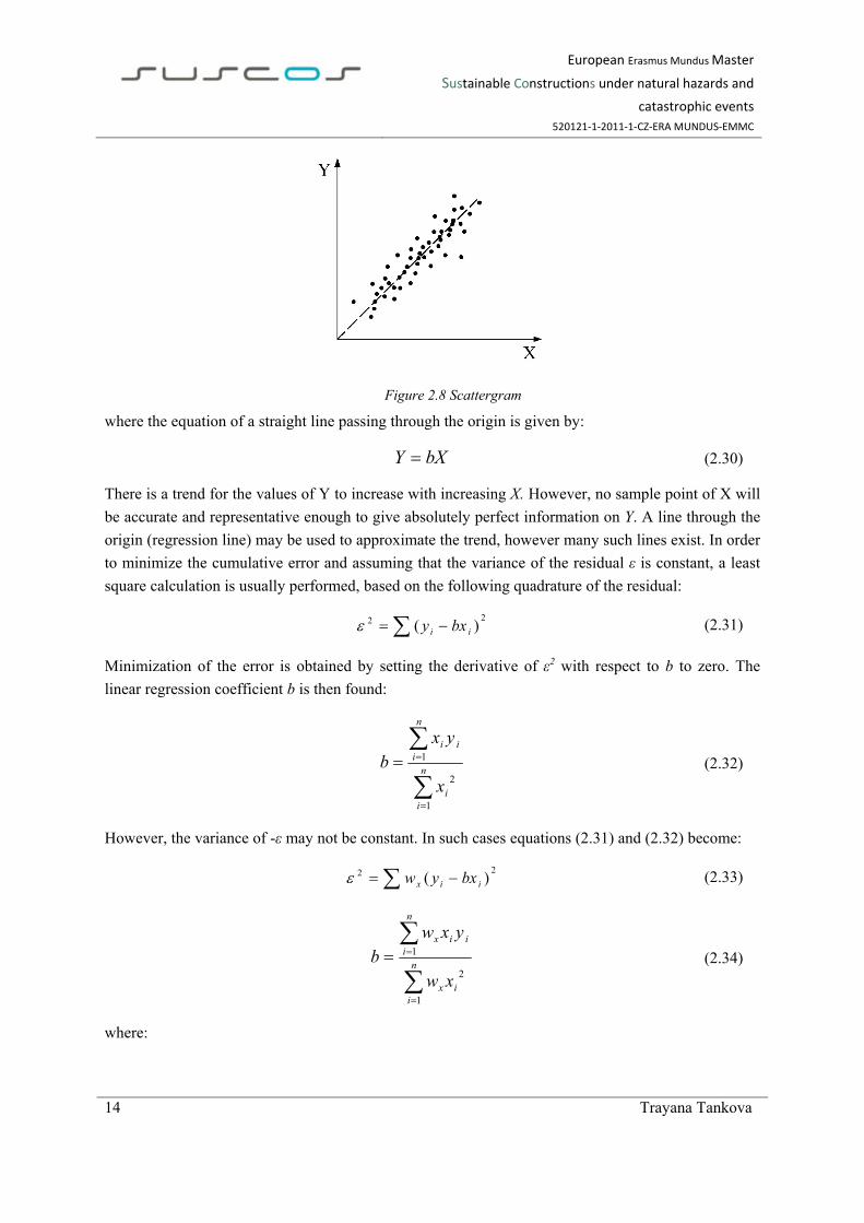
2.8 REGRESSION ANALYSIS
If two random variables are considered, there may be a relationship between them. Moreover, the
presence of randomness makes the relationship not unique and thus it leads to scatter. The two
variables can be plotted together in a scattergram type graph, see Figure 2.8.
European Erasmus Mundus Master
Sustainable Constructions under natural hazards and
catastrophic events
520121‐1‐2011‐1‐CZ‐ERA MUNDUS‐EMMC
14 Trayana Tankova
Figure 2.8 Scattergram
where the equation of a straight line passing through the origin is given by:
bXY (2.30)
There is a trend for the values of Y to increase with increasing X. However, no sample point of X will
be accurate and representative enough to give absolutely perfect information on Y. A line through the
origin (regression line) may be used to approximate the trend, however many such lines exist. In order
to minimize the cumulative error and assuming that the variance of the residual ε is constant, a least
square calculation is usually performed, based on the following quadrature of the residual:
22 )( ii bxy (2.31)
Minimization of the error is obtained by setting the derivative of ε2 with respect to b to zero. The
linear regression coefficient b is then found:
n
ii
n
iii
x
yxb
1
2
1 (2.32)
However, the variance of -ε may not be constant. In such cases equations (2.31) and (2.32) become:
22 )( iix bxyw (2.33)
n
iix
n
iiix
xw
yxwb
1
2
1 (2.34)
where:

European Erasmus Mundus Master
Sustainable Constructions under natural hazards and
catastrophic events
520121‐1‐2011‐1‐CZ‐ERA MUNDUS‐EMMC
Trayana Tankova 15
)(
1
Varwx (2.35)
If w is proportional to X then expression (2.34) can be rewritten as:
x
y
x
y
xxk
xyxkb
n
ii
n
ii
n
iii
n
iiii
1
1
1
2
1
)(
)(
(2.36)
In case that wx is proportional to rt2 then expression (2.34) becomes:
n
ii
n
ii
n
iii
n
iii
n
iiii
x
y
nn
xy
xxk
xyxkb
1
11
1
22
1
2
1
)(
)(
(2.37)
This last assumption is correct if X is proportional to Y, excluding the sampling error. Furthermore,
the three estimators for b (2.32), (2.36) and (2.37) are all unbiased. As it is explained in [4], the choice
of approximation is a question of precision: as the first one should be used when the standard
deviation of the residual is constant (2.32); the second one when the standard deviation of the residual
is proportional to X (2.36); and the third one when the standard deviation of the residual is
proportional to X2 (2.37).


European Erasmus Mundus Master
Sustainable Constructions under natural hazards and
catastrophic events
520121‐1‐2011‐1‐CZ‐ERA MUNDUS‐EMMC
Trayana Tankova 17
3 BASIS OF DESIGN
The structural reliability may be verified using fully probabilistic approach or partial factor method. In
practice, the partial factor method is often applied, since it incorporates the variability in the design
code and offers a clear guidance to the engineer. The fully probabilistic methods are not as frequently
used because usually, there is not sufficient information for their application, moreover the outcome
depends on the person who performs the analysis and therefore the level of safety between different
analyses, would be left undetermined. A model application of design code is given by [5] where the
fully probabilistic approach is adopted.
However, here focus is given to the current structural design codes in Europe are EN 1990 to EN
1999. The basic document of this family of codes is EN 1990 – Basis of structural design [1]. It
establishes principles and requirements for the safety assessment of structures; it describes the basis of
their design and provides guidelines for structural reliability.
In this chapter, a brief introduction to the basis of design as well as its background is presented.
A procedure for design assisted by testing is provided in the scope of EN 1990 – given in its Annex D.
The latter procedure is based on a semi – probabilistic approach. Its theoretical background is also
summarized in the following subsections.
3.1 GENERAL OVERVIEW OF EN 1990
All parts of the Eurocodes are based on the partial safety factor method. EN 1990 states the basis of
the method. The partial safety factor method recognizes relevant design situations. The safety factors
are used on load and on the resistance sides and the design is considered adequate whenever the
appropriate limit states are verified:
dd RE (3.1)
where:
Ed – is the design value of the actions;
Rd – is the design value of the resistance;
The safety factors are established based on a statistical evaluation of experimental data; or based on a
calibration to experience derived from a long building tradition. The partial safety factors should be
calibrated such that the reliability level is as close as possible to the target reliability. The calibration
of safety factors can be performed based on full probabilistic methods, or on First Order Reliability
Methods. The full probabilistic approach is often not possible to use due to the lack of sufficient
statistical data.

European Erasmus Mundus Master
Sustainable Constructions under natural hazards and
catastrophic events
520121‐1‐2011‐1‐CZ‐ERA MUNDUS‐EMMC
18 Trayana Tankova
However, in [6] it is reported that the analysis can be based on the Bayesian interpretation of
probabilities, where the probabilities are evaluated using available data and previous knowledge. It is
believed that if the analysis is carried out carefully and based on large number of data points, the
results would be correct.
Figure 3.1 illustrates the various possible reliability methods according to EN 1990 [1].
Figure 3.1 Possible Reliability methods [1]
The level of safety in EN 1990 is chosen according to Consequence classes (CC) defined in Annex B.
The consequence classes establish the reliability differentiation of the code by considering the
consequence of failure or malfunction of the structure. The Consequence Classes (CC) correspond to
Reliability classes (RC), which define the target reliability level though the reliability index β. This
index defines the probability of failure, given by:
)( fP (3.2)
where Φ is the cumulative distribution function (CDF) for the standard normal distribution.
The reliability index covers the scatter on both resistance and action sides. It can be expressed in
terms of number of standard deviations as shown on Figure 3.2.

European Erasmus Mundus Master
Sustainable Constructions under natural hazards and
catastrophic events
520121‐1‐2011‐1‐CZ‐ERA MUNDUS‐EMMC
Trayana Tankova 19
Figure 3.2 Reliability index β [1]
According to [7], “the target reliability index or the target failure probability is the minimum
requirement for human safety from the individual or societal point of view when the expected number
of fatalities is taken into account. It starts from an accepted lethal accident rate of 10-6 per year,
corresponding to a reliability index 1 = 4.7”. The reference period (the design life) depends on the
Reliability class, i.e. for most of the structures it is 50 years which leads to β=3.8.
The probability of failure as expressed in Eq. (3.2) includes the loading and the resistance parts.
However, EN 1990 allows one to separate the scatter due to loading and resistance in terms of
coefficients αE and αR, respectively (see Figure 3.2), where:
0.122 ER (3.3)
The partial safety factors related to the resistance are determined based on the following expression:
)( rdrrP (3.4)
where r stands for resistance and rd is the design resistance. The factor αR may be assumed to have a
fixed value of 0.8 in case the standard deviation of the load effect and the resistance do not deviate
very much (0.16<σE/σR<7.6) [1]. This simplification is crucial for a standardized determination of the
partial safety factors for the resistance side without the need to simultaneously consider the action
side.

European Erasmus Mundus Master
Sustainable Constructions under natural hazards and
catastrophic events
520121‐1‐2011‐1‐CZ‐ERA MUNDUS‐EMMC
20 Trayana Tankova
3.2 METHODOLOGICAL ASSUMPTIONS FOR DESIGN RESISTANCE
3.2.1 DESIGN RESISTANCE
In Section 6 of EN 1990, three different alternatives for the evaluation of the design resistance are
proposed, as follows:
METHOD 1 (clause 6.3.5(1)):
On the resistance side, the general format is given in expressions (3.5) to (3.8).
1;1
,
,
iaX
RR dim
iki
Rdd
(3.5)
where:
γRd –partial safety factor covering uncertainty in the resistance model, plus geometric deviations
if these are not modeled explicitly;
Xk,i – characteristic value of material property i;
ηi – conversion factor, which can alternatively be incorporated in γM (see expression (3.7));
ad – design value of geometrical data, it can be represented by nominal values in cases not
severely affected by geometrical shape deviations.
nomd aa (3.6)
Expression (3.5) may be simplified as follows:
1;,
,
iaX
RR diM
ikid
(3.7)
(3.8)
Further simplifications may be given for different structural materials but they should not reduce the
level of reliability [1].
i,mRdi,M

European Erasmus Mundus Master
Sustainable Constructions under natural hazards and
catastrophic events
520121‐1‐2011‐1‐CZ‐ERA MUNDUS‐EMMC
Trayana Tankova 21
METHOD 2 (clause 6.3.5(3)):
Alternatively to (3.7), the design resistance may be obtained directly from the characteristic value of
product or material resistance, without explicit determination of the design values for individual basic
variables:
M
kd
RR
(3.9)
The latter is applicable to products or members made of a single material and it is also used in
connection with Annex D of EN 1990. It is noted that this simplified approach is used for the
evaluation of the design resistance of most failure modes in Eurocode 3 [2].
METHOD 3 (clause 6.3.5(4)):
Alternatively to expressions (3.7) and (3.9), for structures or structural members that are analysed by
non-linear methods and comprise more than one material acting together, the following expression
can be used:
1;;1
,
1,,,
,
iaXXRR dim
mikiiki
iMd
(3.10)
In section 2.3.4 of EN 1993-1-1 [2], it is stated that the evaluation of design resistance should be
based on equations (3.9) or (3.10).
The method proposed by expression (3.10) will not be addressed in this study.
3.2.2 PARTIAL FACTORS IN EN 1990
The following partial factors are defined in EN 1990:
- F – Partial factor for actions, also accounting for model uncertainties and
dimensional variations;
- f – Partial factor for actions, which takes account of the possibility of unfavorable
deviations of the action values from the representative values;
- Sd - Partial factor associated with the uncertainty of the action and/or action effect
model;
- M – Partial safety factor for a material property also accounting for model
uncertainties and model variations;

European Erasmus Mundus Master
Sustainable Constructions under natural hazards and
catastrophic events
520121‐1‐2011‐1‐CZ‐ERA MUNDUS‐EMMC
22 Trayana Tankova
- m – Partial factor for a material property;
- Rd – Partial factor associated with the uncertainty of the resistance model;
The relation between individual partial factors in the Eurocodes is schematically shown in Figure 3.3:
Figure 3.3Relation between individual partial factors [1]
In accordance with Figure 3.3 and following [8],
F f Sd (3.11)
M m Rd (3.12)
Expression (3.12) is equal to the one given in (3.8) and may be used in conjunction with (3.7).
3.3 SAFETY ASSESSMENT PROCEDURE – ANNEX D DESIGN ASSISTED BY TESTING
Annex D of EN 1990 gives a semi-probabilistic procedure for the safety assessment of design
methods. According to [8], Annex D distinguishes several types of tests depending on their purpose
that may be classified into the two following categories: (i) results used directly in design; (ii) control
or acceptance tests. According to the objectives here, the procedures for the statistical determination
of resistance models and procedures for deriving design values from tests of type (i) are detailed in the
following.
Various types of uncertainties are present in a resistance model and they are unavoidable. As it is
explained in [3], they can be associated with inaccuracies of the prediction of the reality or with the
European Erasmus Mundus Master
Sustainable Constructions under natural hazards and
catastrophic events
520121‐1‐2011‐1‐CZ‐ERA MUNDUS‐EMMC
Trayana Tankova 23
natural randomness. In order to quantify the uncertainties testing is used. It can be done by numerical
or experimental testing.
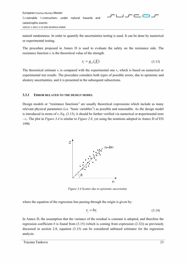
The procedure proposed in Annex D is used to evaluate the safety on the resistance side. The
resistance function rt is the theoretical value of the strength.
)(Xgr rtt (3.13)
The theoretical estimate rt is compared with the experimental one re, which is based on numerical or
experimental test results. The procedure considers both types of possible errors, due to epistemic and
aleatory uncertainties, and it is presented in the subsequent subsections.
3.3.1 ERROR RELATED TO THE DESIGN MODEL
Design models or “resistance functions” are usually theoretical expressions which include as many
relevant physical parameters (i.e. “basic variables”) as possible and reasonable. As the design model
is introduced in terms of rt, Eq. (3.13), it should be further verified via numerical or experimental tests
- re. The plot in Figure 3.4 is similar to Figure 2.8, yet using the notations adopted in Annex D of EN
1990.
Figure 3.4 Scatter due to epistemic uncertainty
where the equation of the regression line passing through the origin is given by:
te brr (3.14)
In Annex D, the assumption that the variance of the residual is constant is adopted, and therefore the
regression coefficient b is found from (3.15) (which is coming from expression (2.32)) as previously
discussed in section 2.8, equation (3.15) can be considered unbiased estimator for the regression
analysis.

European Erasmus Mundus Master
Sustainable Constructions under natural hazards and
catastrophic events
520121‐1‐2011‐1‐CZ‐ERA MUNDUS‐EMMC
24 Trayana Tankova
n
iit
n
iieit
r
rrb
1
2,
1,,
(3.15)
The scatter in Figure 3.4 represents the epistemic uncertainty which is related to the differences that
arise between the adopted design model and the reality. This variation is caused by the simplifications
of every design model when compared to reality.
The differences are considered in terms of the error δi:
10
,
,
,
,
i
it
iit
it
iei
i
rb
rb
rb
r
(3.16)
Assuming that the resistance distribution follows a lognormal distribution, the logarithm of the error δi
is given by:
)ln( ii
(3.17)
The mean value of Δ is found from:
n
iin 1
1 (3.18)
The estimate of the error variance is:
n
iin
s1
22
1
1 (3.19)
Finally, the estimator for the coefficient of variation of the error term δi is given by:
1)exp( 2 sV (3.20)
3.3.2 ERROR RELATED TO THE BASIC INPUT VARIABLES
The aleatory uncertainty, accounting for the natural randomness, is associated with the basic input
variables Xi – yield strength, ultimate strain, geometrical properties, etc.
Considering the correction factor for the model variance, the resistance function (3.13) may be
rewritten as:

European Erasmus Mundus Master
Sustainable Constructions under natural hazards and
catastrophic events
520121‐1‐2011‐1‐CZ‐ERA MUNDUS‐EMMC
Trayana Tankova 25
)...,( 21 nrt XXXbgr (3.21)
Furthermore, as previously presented in section 2.7, approximations about the moments of functions
of random variables, can be found using expressions (2.27) and (2.29) (as proposed in [3]) by
expansion in a Taylor series about the mean values. Hence the following expressions can be found,
using the notations adopted in EN 1990;
If the series is truncated after the linear terms, i.e.,
n
i i
rtimimrt X
gXXbXbgr
1, )()( (3.22)
the first order mean and variance are obtained as follows:
)()( mrt XbgrE (3.23)
2
1
2)(
n
i i
rti X
grVar (3.24)
Expression (3.24) is based on the assumption that the basic variables Xi and Xj are statistically
independent and is obtained from the truncated series of Eq. (2.29) as given in Eq. (3.22), otherwise
more terms shall be included from Eq.(2.28).
The sensitivity of the resistance function to the variability of the basic input parameters is considered
through the coefficient of variation Vrt. In case that the resistance function is not very complex such as
a simple product function, Vrt may be obtained as follows:
n
iiXVarrVar
1
)(ln)(ln (3.25)
n
iixr VV
1, )1ln(1ln (3.26)
2
1
2
k
jxrt VV (3.27a)
However, if the resistance function is expressed by a more complex function, then Vrt should be based
on Eq. (3.24), leading to:
European Erasmus Mundus Master
Sustainable Constructions under natural hazards and
catastrophic events
520121‐1‐2011‐1‐CZ‐ERA MUNDUS‐EMMC
26 Trayana Tankova
2
12
2 1
k
jj
j
j
m
rt X
Xg
XgV (3.27b)
3.3.3 THE PARTIAL SAFETY FACTOR
Finally, both uncertainties are combined in order to obtain the partial safety factor – γM.
Expression (3.28) combines the effect of scatter due to design model and scatter due to the basic
random variables, is obtained similarly to Eq. (3.26):
)1)(1()1( 222 rtr VVV (3.28)
The second order terms may be ignored if the coefficients of variation are small, leading to:
222rtr VVV (3.29)
The standard deviations of the lognormal variables are given by:
)1ln( 2 VQ (3.30)
)1ln( 2 rtrt VQ (3.31)
)1ln( 2 rVQ (3.32)
From a probabilistic stand point, the design value of the resistance should satisfy the following
relation, in case of large number of tests (n>30):
R
rM
k
M
kd Q
r
rrPrrP
ln
(3.33)
λr is the lognormal mean and it can be found using the following relationship:
2
2
1ln Qrmr (3.34)
so that
22 5.05.0 )( QQ
mrtQQ
mM
k RR eXbgerr
(3.35)

European Erasmus Mundus Master
Sustainable Constructions under natural hazards and
catastrophic events
520121‐1‐2011‐1‐CZ‐ERA MUNDUS‐EMMC
Trayana Tankova 27
leading finally to:
25.0)( QQmrt
kM
ReXbg
r
(3.36)
In this way, the design value of the resistance considers both uncertainties – the one due to the scatter
of the basic input variables and the one related with simplifications introduced in the design model. It
also corresponds to the selected reliability level β according to Reliability Classes and the
corresponding Consequence Classes.
The characteristic value of the resistance is the resistance function evaluated at nominal values of the
basic input variables as follows:
)(, nomrtnomtk Xgrr (3.37)
In case of a limited number tests (say n<30) allowance should be made in the distribution of Δ for
statistical uncertainties. The distribution should be considered as a central t-distribution leading to
(3.38a).
The design value of the resistance function based on the mean values of the input parameters is
calculated, depending on the sample size used:
nQQkXbg
nQQ
Qk
Q
QkXbg
r
dmrt
ndrt
dmrt
d
2,
22
,
2
,
5.0exp)(
305.0exp)(
(3.38a)
(3.38b)
Coefficients ,dk and ndk , are design fractile factors, which can be obtained from Table 3.1.
However; it should be noted that Table 2.1 is based on αRβ=3.04.
Table 3.1Values for kd,n
n 1 2 3 4 5 6 8 10 20 30 ∞
VX
known 4.36 3.77 3.56 3.44 3.37 3.33 3.27 3.23 3.16 3.13 3.04
VX
unknown - - - 11.40 7.85 6.36 5.07 4.51 3.64 3.44 3.04

European Erasmus Mundus Master
Sustainable Constructions under natural hazards and
catastrophic events
520121‐1‐2011‐1‐CZ‐ERA MUNDUS‐EMMC
28 Trayana Tankova
The partial safety factor is then found:
d
nomtM r
r ,* (3.39)
The procedure proposed in Annex D of EN 1990 is summarized in Figure 3.5:

European Erasmus Mundus Master
Sustainable Constructions under natural hazards and
catastrophic events
520121‐1‐2011‐1‐CZ‐ERA MUNDUS‐EMMC
Trayana Tankova 29
Figure 3.5Flow chart – Annex D


European Erasmus Mundus Master
Sustainable Constructions under natural hazards and
catastrophic events
520121‐1‐2011‐1‐CZ‐ERA MUNDUS‐EMMC
Trayana Tankova 31
4 ALTERNATIVES FOR SAFETY ASSESSMENT
4.1 ASSUMPTIONS
The procedures described in section 3.3 are of general application. Consequently, since they have to
cover different types of materials and different types of problems, they provide many alternative
possibilities, leading to several possible implementations for a given problem. Furthermore, the
framework is also necessarily complex, leading to difficult implementation in certain cases. These
constitute a difficulty whenever it is necessary to compare two alternative design rules because
different implementations will lead to different failure probabilities even when the basic data is the
same. Also, very often, the available data is not sufficient to characterize statistically all the relevant
basic variables. Finally, carrying out a probabilistic analysis that includes all the relevant variability’s
may be impossible because of the size of the required sample [9].
In this chapter, various procedures for the implementation of the methodology of Annex D are
presented. They include a number of simplifications, starting from the simplest to the most complex
and are proposed in the context of design models for the evaluation of the buckling resistance of steel
members.
Without loss of generality, in the following, it is assumed that a large number of experiments is
available (at least 100 results). Also, whenever it is necessary to exemplify some detail using a
specific stability phenomenon, the well-known example of flexural buckling of columns is used.
In the context of the stability of steel structures, the following basic variables should be considered for
the evaluation of the error related to the basic input variables (Vrt):
- mechanical properties of steel
- cross section and member dimensions
- geometrical imperfections
- residual stresses
- load eccentricity.
In steel structures, the variability of these variables contributes differently to the buckling resistance
of steel members:
- the variability of the mechanical properties of steel has a significant relevance, in
particular the yield stress. They should be considered as random variables,
bearing in mind that the nominal properties of steel are guaranteed values.

European Erasmus Mundus Master
Sustainable Constructions under natural hazards and
catastrophic events
520121‐1‐2011‐1‐CZ‐ERA MUNDUS‐EMMC
32 Trayana Tankova
- the variability of the cross section dimensions and member lengths may be
considered small or negligible in most cases [8]. However, if a systematic
deviation from nominal values is identified, they should also be considered as
random variables.
- The remaining basic variables listed above (geometric imperfections, residual
stresses and load eccentricities) have a crucial effect on the buckling resistance.
They could be considered explicitly as random variables in the design model but,
because of the complexity of the stability design models, they do not appear
explicitly in the stability design expressions. Consequently, they are usually
considered implicitly in the models. Whenever relevant (e.g. advanced numerical
models), these imperfections should be represented directly by their design values
(clause 4.3(1) of EN 1990) or by values corresponding to some prescribed fractile
of the available statistical distributions (clause 4.3(3) of EN 1990).
The different alternatives presented in this chapter consider the variability of the (geometrical,
material and loading) imperfections implicitly in the models. Hence, the first level of simplifications
presented below consists of neglecting the error related to the first two basic variables, i.e., material
and geometry. Table 4.1 summarizes the assumptions for each proposed simplified procedure.
Table 4.1 Simplified procedures
P0 P1 P2
Mech. Properties of steel
(yield stress)
X (approx.)
X X
Geometry X
Finally, it is noted that as a reference simplification, PROCEDURE 0 only considers model
uncertainty and material (yield stress) uncertainties and calculates independently the partial safety
factors for each of them according to expression (3.12) while the other two follow strictly the
methodology of Annex D of EN 1990.

European Erasmus Mundus Master
Sustainable Constructions under natural hazards and
catastrophic events
520121‐1‐2011‐1‐CZ‐ERA MUNDUS‐EMMC
Trayana Tankova 33
4.2 PROCEDURE 0 (P0)
Figure 4.1 summarizes procedure P0. It only considers model uncertainty and material (yield stress)
uncertainty and calculates independently (in an approximate way) the partial safety factors for each of
them [9],[10]. Hence, (3.38b) is used with nominal values of material and geometrical properties
leading to:
2,
,
5.0exp
1
QQkRr
r
ndmd
nomtRd
(4.1)
The material variability is considered independently from the design model and it is evaluated
separately as follows:
)V64.11(f
f
fym,y
nom,ym (4.2)
Figure 4.1 - Procedure 0

European Erasmus Mundus Master
Sustainable Constructions under natural hazards and
catastrophic events
520121‐1‐2011‐1‐CZ‐ERA MUNDUS‐EMMC
34 Trayana Tankova
Geometry is assumed with nominal values.
According to Figure 4.1, Step 2, the following assumption is adopted in the construction of the
regression line:
n
i i,t
i,em r
r
nR
1
1 (4.3)
This was applied in [9],[10], as previously proposed by [11] and [12]. It is noted that the adoption of
different estimators for the regression line is a matter of precision. However, as the sample size tends
to infinity, the difference between estimators becomes negligible [4].
It is further noted that Procedure 0 presents some drawbacks for the evaluation of partial safety
factors for stability problems, since it considers γRd and γm with the same weight, which is not true in
cases with high slenderness. Nevertheless, besides its simplicity, it may be considered for other failure
modes, e.g. ductile failure modes driven by plasticity. Finally, P0 does not ensure strict compliance
with a predefined target failure probability.
4.3 PROCEDURE 1 (P1)
4.3.1 DESCRIPTION
This procedure was also applied in [9],[10]. It constitutes a simplification of Annex D and also
disregards the variability of geometry (ad = anom). It is performed on the basis of expression (3.9). The
procedure is summarized in Figure 4.2.
A further simplification is introduced with regard to the coefficient of variation of the (error of the)
resistance function, Vrt, using expression (3.27a). It is simply assumed to be equal to the coefficient of
variation of the yield strength. Annex D explicitly allows such assumption in cases where the
resistance function is described by a simple product function, as explained before.
2
222
ym
fyfyrt f
VV
(4.4)

European Erasmus Mundus Master
Sustainable Constructions under natural hazards and
catastrophic events
520121‐1‐2011‐1‐CZ‐ERA MUNDUS‐EMMC
Trayana Tankova 35
Figure 4.2 - Procedure 1
The assumption of fy as the only basic variable (P1) is expected to be more inaccurate within the high
slenderness range for stability problems, due to the fact that yield strength has no significant
importance in that range. However, it is considered to be more adequate than P0 since it accounts for
the propagation of the variability of the yield strength in the resistance function.
4.3.2 ASSESSMENT OF THE CONSERVATIVE NATURE OF PROCEDURE 1
Comparing P1 with the Annex D procedure and assuming that only the model and the yield stress
variabilities are explicitly considered, the only difference consists then on the evaluation of Vrt. It
would be useful if it could be proven that P1 is a safe-sided approach with regard to Annex D and also
that the differences between the two methods are not significant. This is analytically proven in this

European Erasmus Mundus Master
Sustainable Constructions under natural hazards and
catastrophic events
520121‐1‐2011‐1‐CZ‐ERA MUNDUS‐EMMC
36 Trayana Tankova
subsection for a realistic range of yield stress distribution and assumed realistic values of the model
variability.
Consider expression (3.36) that yields the partial safety factor M :
2,
*
5.0exp)(
)(
QQkXbg
Xg
dmrt
nomrt
M
(4.5)
Comparing P1 with Annex D shows that he terms )(),(, nomrtmrt XgXgb are the same regardless of
the method used. Therefore, any differences between the two procedures are solely related to the
following expression:
2, 5.0exp
1
QQkd
(4.6)
In addition, the procedure of Annex D evaluates partial safety factors *,iM for each specimen, while
P1 computes directly a total value for the sample. However, here, each value i, will be compared to
the total value of P1.
The following assumption is considered: large number of test results – more than 100.
The following notation is adopted:
The coefficient of variation Vrt calculated using the procedure of Annex D with partial
derivatives is henceforth denoted as Vrt,D;
The coefficient of variation Vrt calculated using Procedure 1 is henceforth denoted as Vrt,1;
)1VVln(Q 2D,rt
2D (4.7)
)1ln( 21,
21 rtVVQ (4.8)
The derivative of Q with respect to Vrt is:

European Erasmus Mundus Master
Sustainable Constructions under natural hazards and
catastrophic events
520121‐1‐2011‐1‐CZ‐ERA MUNDUS‐EMMC
Trayana Tankova 37
00)1ln()1( 2222
rt
rtrt
rt
rt
VVVVV
V
V
Q
(4.9)
Since it is larger or equal to zero for any Vrt, Q is a monotonically increasing function and the
following conclusion may be drawn:
)()( 2,,1,, rtDrtthen
rtDrt VQVQVVIf (4.10)
Differentiating expression (4.6) with respect to Q yields:
2,d2
,d
Q5.0QkexpQ5.0Qkexp
1
00)(5.0exp5.0exp
,2
,
2,
QkQQQkdQ
QQkddd
d
Since it is larger or equal to zero for all Q, the function is also monotonically increasing, then
211,
2,
1,,5.0exp
1
5.0exp
1)()(
QQkQQkVQVQIf
dDDd
thenrtDrt
(4.11)
Combining (4.10) and (4.11), it can be concluded that if it can be proven that 1,, rtDrt VV then the
values of γM obtained with P1 would be a safe-sided estimate of the partial safety factor.
In order to compare Vrt,D and Vrt,1, a resistance function needs to be assumed. Considering the
formulation of EN 1993 [2] for the flexural buckling of columns leads to:
AfffgXg yyfyrtirt )()()( (4.12)
Differentiating the resistance function with respect to the yield stress fy, gives:
AfAfdf
fd
df
fdgyy
y
y
y
yrt ).()()(
(4.13)
The coefficient of variation Vrt is evaluated by:
)f(
)f(fdf
)f(d
f
σσ
df
)(fdg
)(fg
1V
ym
yyy
y
2ym
2fy2
fy
2
y
yrt
ym2
rt
2rt 2
2
(4.14a)

European Erasmus Mundus Master
Sustainable Constructions under natural hazards and
catastrophic events
520121‐1‐2011‐1‐CZ‐ERA MUNDUS‐EMMC
38 Trayana Tankova
Vrt ,12
fy2
fym2 (4.14b)
Dividing (3.13a) by (3.13b) yields:
)(
)()(
2
2
ym
yyy
y
f
ffdf
fd
C
(4.15)
The derivative of χ with respect to fy is found:
22
222
)()(
)(5.0)()(5.0)(
)()()()(
)(
yy
yyyy
y
yyyy
y
y
ff
ffff
df
fdfff
df
fd
It can be seen that it is lower than zero for any value of the yield stress, because it is a decreasing
function.
0)(
yy
y fdf
fd
The numerator and the denominator of the ratio C from expression (4.15) are plotted on Figure 4.3. In
order to be able to analyse the value of C, these quantities have to be measured separately, since
different values of the yield stress enter the equation: the specimen i value of fy,, fy,i, is present in the
numerator, while the mean value of fy, fy,m, is present in the denominator.

European Erasmus Mundus Master
Sustainable Constructions under natural hazards and
catastrophic events
520121‐1‐2011‐1‐CZ‐ERA MUNDUS‐EMMC
Trayana Tankova 39
Figure 4.3 - Analysis of denominator (yellow curve) and numerator (blue curve) of Ratio C
A fully analytical proof of the conservatism of ratio C is not possible, since different values of the
yield stress have to be assumed – i.e. fy,m≠fy,i. However, it can be proven that only an unrealistic
distribution of the yield stress will lead to C higher than unity. Firstly, let us notice that the ratio C is
smaller than unity whenever fy,i=fym, or fy,i>fym. However, when the mean value of the yield stress is
higher than the one for a certain specimen, this does not necessarily occur: when fy,i<fym, this leads to a
lower value of the normalized slenderness and consequently a higher χ for this specimen. In such case
it should be checked if the ratio remains lower than unity. Nevertheless, by observing Figure 4.3, it
can be seen that this is unlikely to occur and only a distribution with an unrealistic high scatter of the
yield strength would lead to such a situation. For example, if an extreme case is considered when the
minimum value of fyi=fynom, since the absolute minimum of the yield stress is nominal (guaranteed
value), then both terms of the ratio C become equal:
)()()(
2
2
,,,
,ymiyiy
iy
iy fffdf
fd
(4.16)
By going through all slenderness ranges of )( ,iyf , one can obtain )( ,myf by combining equations
(4.16) and (4.17) and consequently can extract the value of fy,m that leads to such normalized
slenderness. This was carried out considering all imperfection factors α from EC3-1-1. The minimum
0
0.1
0.2
0.3
0.4
0.5
0.6
0.7
0.8
0.9
1
0.2 0.4 0.6 0.8 1 1.2 1.4 1.6 1.8 2 2.2 2.4
λ
χ2
[dχ/dfy*fy+χ]2
)( ,myf
)( ,iyf

European Erasmus Mundus Master
Sustainable Constructions under natural hazards and
catastrophic events
520121‐1‐2011‐1‐CZ‐ERA MUNDUS‐EMMC
40 Trayana Tankova
difference between fy,i and fy,m was observed for 7.0)( , iyf and 0.941)( , myf , buckling curve
a0. This leads to fy,m= 424.52 MPa when fy,i=235 MPa (guaranteed value). Because the yield stress
follows a log-normal distribution, the consideration of such parameters leads to a coefficient of
variation of CoV=14.6% which is unlikely to occur. The CoV. value is determined as follows:
1) Fistly, fy,i = 235 MPa is assumed as the value for which the probability of finding a lower fy,i
approaches zero. With this, the mean and standard deviation of the correspondent normal
distribution can be found:
)ln(4
040)ln(
)(
,
,,
iy
iyiy
f
ffXP
(4.17)
where the value of the x=-4 such that the CDF 0 x can be retrieved from standard
normal distribution tables.
2) Secondly, the following set of equations to transform a lognormal distribution
fyymfLogN ; in a normal distribution ;N is used:
2
2
2
5.0ln
1ln
ym
ym
fy
f
f (4.18)
3) Finally, considering fy,i=235 MPa, and replacing Eq. (4.17) in Eq (4.18), the
ymfy fCoV can be found.
4.4 PROCEDURE 2 (P2)
This procedure also constitutes a simplification of Annex D that can be considered as an extension of
Procedure 1 as it now considers explicitly the variability of the geometry (see Figure 4.4). It is based
on expression (3.9). It considers both variability of material and cross-section, so that the coefficient
of variation Vrt is now calculated as:
222csfyrt VVV (4.19)

European Erasmus Mundus Master
Sustainable Constructions under natural hazards and
catastrophic events
520121‐1‐2011‐1‐CZ‐ERA MUNDUS‐EMMC
Trayana Tankova 41
Steel profiles are available in multiple cross sectional shapes ranging from tubular profiles or I and H
cross sections to arbitrary cross section shapes. The geometry of a generic cross section is defined by
the shape and pairs of values for thickness and width (ti, bi). Although the statistical characterization
of the variability of the cross section geometry must be done for each individual family of profiles, the
buckling resistance formulas are written as a function of cross sectional properties (area, elastic or
plastic moduli, moments of inertia). Consequently, it is possible to consider either the basic
dimensions or directly the relevant geometrical properties as the random variables. The latter option is
certainly better from a practical point of view. In both cases, the coefficient of variation Vcs may be
written in a more general way as:
k
jxcs VV
1
22
(4.20)
Figure 4.4 - Procedure 2
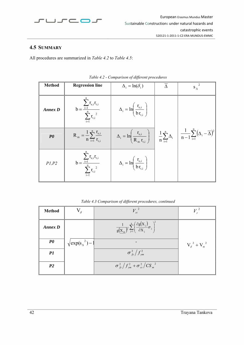
European Erasmus Mundus Master
Sustainable Constructions under natural hazards and
catastrophic events
520121‐1‐2011‐1‐CZ‐ERA MUNDUS‐EMMC
42 Trayana Tankova
4.5 SUMMARY
All procedures are summarized in Table 4.2 to Table 4.5:
Table 4.2 - Comparison of different procedures
Method Regression line )ln( ii 2s
Annex D
n
1i
2i,t
n
1ii,ti,e
r
rrb
i,t
i,ei rb
rln
n
1iin
1
n
1i
2
i1n
1
P0
n
1i i,t
i,em r
r
n
1R
i,tm
i,ei rR
rln
P1,P2
n
1i
2i,t
n
1ii,ti,e
r
rrb
i,t
i,ei rb
rln
Table 4.3 Comparison of different procedures, continued
Method V 2rtV 2
rV
Annex D
1)sexp( 2
2
k
1jj
j
j
2m
X
Xg
Xg
1
2rt
2 VV P0 -
P1 22
ymfy f
P2 2222
mcsymfy CSf

European Erasmus Mundus Master
Sustainable Constructions under natural hazards and
catastrophic events
520121‐1‐2011‐1‐CZ‐ERA MUNDUS‐EMMC
Trayana Tankova 43
Table 4.4 - Comparison of different procedures, continued
Method Q rtQ Q
Annex D
)1Vln( 2
)1Vln( 2rt
)1Vln( 2r P0 -
P1, P2 )1Vln( 2rt
Table 4.5 - Comparison of different procedures, continued
Method nom,tr dr *M
Annex D
)X(g nomrt
nQ5.0Qkexp)X(bg
30nQ5.0Q
Qk
Q
Qkexp)X(bg
2,dmrt
22
n,d
2rt
,dmrt
d
nom,t
r
r
P0
nQ5.0Qkexp)X(gR
30nQ5.0Q
Qk
Q
Qkexp)X(gR
2,dnomrtm
22
n,d
2rt
,dnomrtm
i,mRdi,M
)V04.31(f
f
r
r
fym,y
nom,y
d
nom,t
P1, P2
nQ5.0Qkexp)X(bg
30nQ5.0Q
Qk
Q
Qkexp)X(bg
2,dmrt
22
n,d
2rt
,dmrt
d
nom,t
r
r

European Erasmus Mundus Master
Sustainable Constructions under natural hazards and
catastrophic events
520121‐1‐2011‐1‐CZ‐ERA MUNDUS‐EMMC
Trayana Tankova 45
5 NUMERICAL VALIDATION OF POSSIBLE ALTERNATIVES
5.1 INTRODUCTION
In this chapter, the various procedures are assessed in the context of the flexural buckling resistance of
steel columns. Because the buckling resistance of steel members presents distinctive behaviours for
the various slenderness ranges, all comparisons are carried out for the slenderness interval [0.2 – 2.5].
The following methodology is adopted to implement the comparative assessment:
(i) assumed statistical distributions for the basic input variables are adopted, which are
plausible representations of the reality;
(ii) the coefficient of variation of the design model Vδ is assumed and varied from 0% to
10%;
(iii) in order to assess the compatibility of the test population, it is split into several sub-
sets according to slenderness intervals;
(iv) the “resistance function” formulation for flexural bucking of columns, section 6.3.1 of
EC3-1-1[2] is considered;
(v) a large number of experiments are available (at least 100).
In this chapter the following basic input variables are used:
Yield strength – fy;
Cross-section area – A;
Second moment of area – I;
Modulus of elasticity – E;
The following cases are analysed and compared:
Procedure 1 – fy (regarding the basic input variables, only fy is considered as a random
variable);
Procedure 2 – fy + A (in accordance with the discussion in section 3.4, besides fy, only
the area is considered as a random variable since for flexural buckling of columns it is a
primary variable);
Procedure 2 – fy+A+I (also I (implicit variable within reduction factor ) is considered
as a random variable);

European Erasmus Mundus Master
Sustainable Constructions under natural hazards and
catastrophic events
520121‐1‐2011‐1‐CZ‐ERA MUNDUS‐EMMC
46 Trayana Tankova
Procedure 2 – fy+A+I+E (also I and E (implicit variables within reduction factor ) are
considered as a random variables);
The above notation is henceforth used to distinguish the various cases.
The results of the application of the simplified procedures P1 and P2 are compared with the Annex D
results in two ways:
- comparison with Annex D results assuming the same random variables: this
comparison is aimed at establishing the conservative nature of the simplification
of using expression (3.27a) instead of (3.27b).
- comparison with Annex D results using all the relevant basic input variables as
random variables: this comparison is aimed at establishing the level of safety of
the simplified procedures.
5.2 GENERATION OF SAMPLES
5.2.1 YIELD STRENGTH
The population of the yield stress can be represented by a lognormal distribution [10].
Three fictitious samples are generated. They are aimed at studying the influence of the scatter of yield
strength on the resistance function. Therefore, all samples have nominal yield strength of 235MPa, the
same mean value of 297.3 MPa, but different standard deviations. The assumptions are summarized in
Table 5.1.
In order to simulate a lognormal distribution, the following transformation was again performed:
2
2
2
5.0ln
1ln
ym
ym
fy
f
f (5.1)
Table 5.1- Assumed descriptors of the yield strength distributions
fym σfy λ ξ
MPa MPa - -
X1 (n=100) 297.3 25 5.691219 0.083942X2 (n=100) 297.3 17.1 5.69309 0.05747X3 (n=100) 297.3 9 5.694284 0.030266
Steel

European Erasmus Mundus Master
Sustainable Constructions under natural hazards and
catastrophic events
520121‐1‐2011‐1‐CZ‐ERA MUNDUS‐EMMC
Trayana Tankova 47
Each sample consists of 100 specimens. Figure 5.1 to Figure 5.3 show the generated values of fy in
the form of histograms.
Figure 5.1 - Histogram X1(S235), fym=297.3MPa, σfy=25MPa
Figure 5.2 - Histogram X2(S235), fym=297.3MPa, σfy=17.1MPa

European Erasmus Mundus Master
Sustainable Constructions under natural hazards and
catastrophic events
520121‐1‐2011‐1‐CZ‐ERA MUNDUS‐EMMC
48 Trayana Tankova
Figure 5.3 - Histogram X3(S235) fym=297.3MPa, σfy=9MPa
5.2.2 GEOMETRICAL PROPERTIES
Hypothetical samples are simulated for the cross-sectional area and moment of inertia. The
distributions are normal and the mean and standard deviation are assumed to follow expressions (5.2)
[13]. Each distribution consists of 100 specimens. The cross section used in this example is an IPE
200.
xx
nomx X
04.0;01.0
99.0 (5.2)
Table 5.2 summarizes the assumptions.
Table 5.2 - Assumed descriptors of cross-section properties distributions
Xnom Xm σX
mm2(mm4) mm2(mm4) mm2(mm4)
A (n=100) 2848 2819.52 112.7808I (n=100) 1424000 1409760 56390.4
Param.

European Erasmus Mundus Master
Sustainable Constructions under natural hazards and
catastrophic events
520121‐1‐2011‐1‐CZ‐ERA MUNDUS‐EMMC
Trayana Tankova 49
Figure 3.1 - Normal distribution of Area, n=100
Figure 3.2 - Normal distribution of moment of inertia, n=100
5.2.3 MODULUS OF ELASTICITY
In order to study the influence of the modulus of elasticity, a sample is generated with 100 specimens.
The distribution is assumed as normal Gaussian with c.o.v. of 5% [7].
Table 5.3 - Assumed descriptors of modulus of elasticity distribution
Xnom Xm σX
MPa MPa MPa
E (n=100) 210000 210000 10500
Param.

European Erasmus Mundus Master
Sustainable Constructions under natural hazards and
catastrophic events
520121‐1‐2011‐1‐CZ‐ERA MUNDUS‐EMMC
50 Trayana Tankova
Figure 3. 3 - Normal distribution of modulus of elasticity
5.3 RESULTS
5.3.1 METHODOLOGY
In this section the result of the numerical assessment of the simplified procedures is presented. The
assessment is performed on the basis of the previously generated distributions. For all cases the
sample size is 100 specimens so that the partial safety factor γM can be obtained from expression
(3.36):
2,
*
5.0exp)(
)(
QQkXbg
Xg
dmrt
nomrt
M
(5.3)
As already mentioned in chapter 4, )(),(, nomrtmrt XgXgb are the same regardless of the method
used. Therefore, the following term can be isolated and used for comparison of the resulting partial
safety factors:
2, 5.0exp
1
QQkd
(5.4)
Using expression (3.27b) coefficients of variation Vrt are calculated for each data point i, yet
simplified procedures propose a single value for the sample.
Finally, the safety factor given by each approach is determined as follows:
(i) When procedures P1 and P2 are used, a global value of M from expression (5.3) is
obtained for the whole sample;

European Erasmus Mundus Master
Sustainable Constructions under natural hazards and
catastrophic events
520121‐1‐2011‐1‐CZ‐ERA MUNDUS‐EMMC
Trayana Tankova 51
(ii) When Annex D is used with Eq. (3.27b), different values of M from expression (5.3)
are obtained for each specimen due to the variation of the basic input variables. As a
result, in order to get a comparable result from expression (5.3) for both alternatives,
the mean value of the single (specimen) results from expression (5.3) is determined.
In the subsequent sub-sections the ratio (5.4) is used to compare different values of the partial
safety factor.
5.3.2 NUMERICAL ASSESSMENT OF P1
In this sub-section, the behavior of P1 in case of flexural column buckling is studied.
In order to compare P1 with the procedure of Annex D when all basic input variables are taken into
account, it is assumed:
- Distribution of the yield strength fy – X2(S235), presented in sub-section 5.2.1;
- Distributions of the area A and moment of inertia I – presented in sub-section 5.2.2;
- Distribution of the modulus of elasticity E – presented in sub-section 5.2.3;
The coefficient of variation of the model is assumed – Vδ=0.05; The results are plotted in Figure 5.4.
The Annex D procedure is presented in terms of each specimen i and the corresponding mean value
(in orange). Additionally, results are given in case fy is assumed as the only random variable in the
Annex D procedure (in red). It can be observed that P1 presents some unsafe results when compared
to the “full” Annex D. On the contrary, when compared to Annex D (fy), it is always safe.

European Erasmus Mundus Master
Sustainable Constructions under natural hazards and
catastrophic events
520121‐1‐2011‐1‐CZ‐ERA MUNDUS‐EMMC
52 Trayana Tankova
Figure 5.4 - Results for distribution X2(S235), Vδ =0.05
A further comparison is performed on the basis of different values of the variability of the model, Vδ.
The results are plotted in terms of percentage difference between partial safety factors evaluated using
P1 and the “full” Annex D (when basic input variables are fy+A+I+E). The “unsafe” trend is
maintained for different Vδ as shown in Figure 5.5.
Figure 5.5 - P1(fy) for various Vδ
It should be mentioned that the percentage difference strongly depends on the distributions that are
being used and Figure 5.5 cannot be taken as a reference case for flexural buckling of columns. It
aims to be illustrative for the problem.
1.15
1.2
1.25
1.3
1.35
1.4
0.2 0.7 1.2 1.7 2.2
1/ex
p(-k
d,nQ
-0,5
Q2 )
Slenderness, λnom
P1 (fy)AnnexD (fy,i)Mean AnnexD (fy,i)AnnexD (fy,i+Ai+Ii+Ei)Mean AnnexD (fy,i+Ai+Ii+Ei)
-4.0%
0.0%
4.0%
8.0%
12.0%
16.0%
0 0.5 1 1.5 2 2.5
[γM
P1/γ M
,Ann
exD
-1]
x100
%
Slenderness, λnom
P1 (fy) vs AnnexD(fy+A+I+E)
0
0.01
0.02
0.03
0.04
0.05
0.06
0.07
0.08
0.09
0.1

European Erasmus Mundus Master
Sustainable Constructions under natural hazards and
catastrophic events
520121‐1‐2011‐1‐CZ‐ERA MUNDUS‐EMMC
Trayana Tankova 53
The influence of the standard deviation of the yield strength is additionally analysed. The samples
presented in sub-section 5.2.1 are used. Procedure P1 is compared with the procedure of Annex D,
when partial derivatives are evaluated only for the yield strength fy, so that the impact of the other
basic variables is omitted. The comparison is performed on the basis of expression (5.4). The
coefficient of variation Vδ is assumed equal to 0.05 for all three cases.
It can be noticed that the variation of the yield stress has more significant influence within the low to
intermediate slenderness range. It is also remarked that P1 would always give higher results when
compared to Annex D if the yield strength were indeed the only variable of the problem, thus
confirming the analytical derivation proposed in sub-section 4.3.2.
Figure 5.6 - Results for distribution X1(S235), Vδ =0.05
1.15
1.17
1.19
1.21
1.23
1.25
1.27
1.29
0.2 0.7 1.2 1.7 2.2
1/ex
p(-k
d,nQ
-0,5
Q2 )
Slenderness, λnom
P1 (fy)
AnnexD (fy,i)
Mean AnnexD (fy,i)
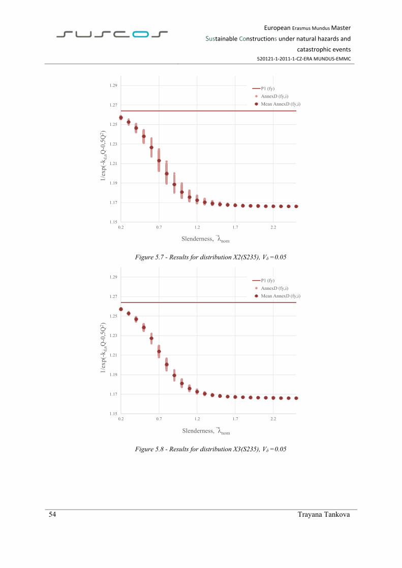
European Erasmus Mundus Master
Sustainable Constructions under natural hazards and
catastrophic events
520121‐1‐2011‐1‐CZ‐ERA MUNDUS‐EMMC
54 Trayana Tankova
Figure 5.7 - Results for distribution X2(S235), Vδ =0.05
Figure 5.8 - Results for distribution X3(S235), Vδ =0.05
1.15
1.17
1.19
1.21
1.23
1.25
1.27
1.29
0.2 0.7 1.2 1.7 2.2
1/ex
p(-k
d,nQ
-0,5
Q2 )
Slenderness, λnom
P1 (fy)
AnnexD (fy,i)
Mean AnnexD (fy,i)
1.15
1.17
1.19
1.21
1.23
1.25
1.27
1.29
0.2 0.7 1.2 1.7 2.2
1/ex
p(-k
d,nQ
-0,5
Q2 )
Slenderness, λnom
P1 (fy)
AnnexD (fy,i)
Mean AnnexD (fy,i)

European Erasmus Mundus Master
Sustainable Constructions under natural hazards and
catastrophic events
520121‐1‐2011‐1‐CZ‐ERA MUNDUS‐EMMC
Trayana Tankova 55
5.3.3 NUMERICAL ASSESSMENT OF P2
For the numerical assessment of P2 in case of the flexural buckling of columns the influence of the
consideration of several random variables related to geometry or related to properties are considered,
as already described in section 5.1. Specifically, the following basic variables are included: cross-
section area, moment of inertia and Young’s modulus. The following cases are analysed:
P2 – fy + A versus Annex D with variability of fy+A; (Figure 5.9)
P2 – fy+A+I versus Annex D with variability of fy+A+I; (Figure 5.10)
P2 – fy+A+I+E versus Annex D with variability of fy+A+I+E; (Figure 5.11)
Assumptions:
- Distribution of the yield strength fy – X2(S235), presented in sub-section 5.2.1;
- Distributions of the area A and second moment of area I – presented in sub-section
5.2.2;
- Distribution of the modulus of elasticity E – presented in sub-section 5.2.3;
- All alternatives are compared with the corresponding assumption for Annex D for
Vδ=0.05;
Firstly, the alternatives are compared to the full Annex D procedure using expression (5.4) similarly
to the previous section, in order to see the deviations between the different assumptions. Unlike P1,
the presence of geometrical properties and Young’s modulus leads to results that are always on the
safe-side.
However, it is observed that as more variables are included, the differences with Annex D become
higher. This issue is associated to the fact that simplified procedures are only adding the variability of
each parameter. On the contrary, the Annex D procedure using partial derivatives takes into account
the variability of each parameter as they appear in the “resistance function”.
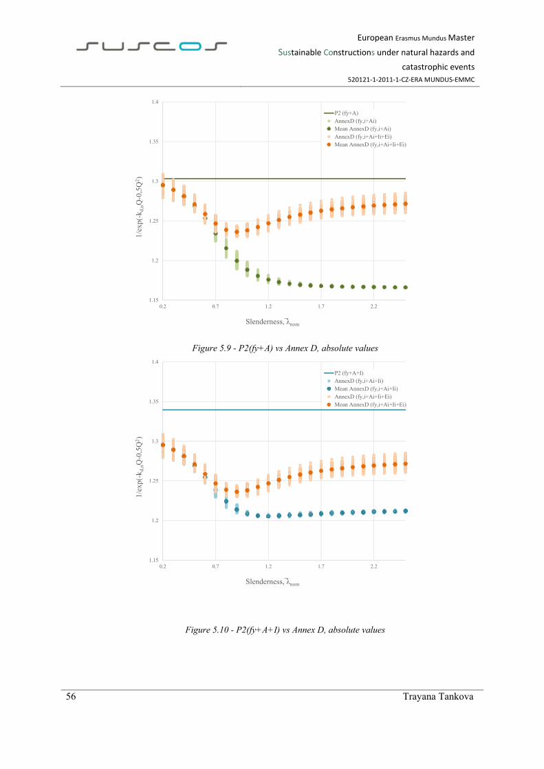
European Erasmus Mundus Master
Sustainable Constructions under natural hazards and
catastrophic events
520121‐1‐2011‐1‐CZ‐ERA MUNDUS‐EMMC
56 Trayana Tankova
Figure 5.9 - P2(fy+A) vs Annex D, absolute values
Figure 5.10 - P2(fy+A+I) vs Annex D, absolute values
1.15
1.2
1.25
1.3
1.35
1.4
0.2 0.7 1.2 1.7 2.2
1/ex
p(-k
d,nQ
-0,5
Q2 )
Slenderness, λnom
P2 (fy+A)AnnexD (fy,i+Ai)Mean AnnexD (fy,i+Ai)AnnexD (fy,i+Ai+Ii+Ei)Mean AnnexD (fy,i+Ai+Ii+Ei)
1.15
1.2
1.25
1.3
1.35
1.4
0.2 0.7 1.2 1.7 2.2
1/ex
p(-k
d,nQ
-0,5
Q2 )
Slenderness, λnom
P2 (fy+A+I)AnnexD (fy,i+Ai+Ii)Mean AnnexD (fy,i+Ai+Ii)AnnexD (fy,i+Ai+Ii+Ei)Mean AnnexD (fy,i+Ai+Ii+Ei)
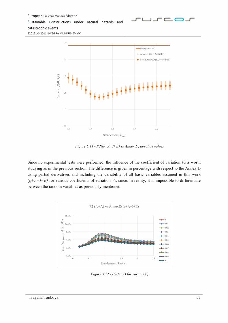
European Erasmus Mundus Master
Sustainable Constructions under natural hazards and
catastrophic events
520121‐1‐2011‐1‐CZ‐ERA MUNDUS‐EMMC
Trayana Tankova 57
Figure 5.11 - P2(fy+A+I+E) vs Annex D, absolute values
Since no experimental tests were performed, the influence of the coefficient of variation Vδ is worth
studying as in the previous section. The difference is given in percentage with respect to the Annex D
using partial derivatives and including the variability of all basic variables assumed in this work
(fy+A+I+E) for various coefficients of variation Vδ, since, in reality, it is impossible to differentiate
between the random variables as previously mentioned.
Figure 5.12 - P2(fy+A) for various Vδ
1.15
1.2
1.25
1.3
1.35
1.4
0.2 0.7 1.2 1.7 2.2
1/ex
p(-k
d,nQ
-0,5
Q2 )
Slenderness, λnom
P2 (fy+A+I+E)
AnnexD (fy,i+Ai+Ii+Ei)
Mean AnnexD (fy,i+Ai+Ii+Ei)
-4.0%
0.0%
4.0%
8.0%
12.0%
16.0%
0 0.5 1 1.5 2 2.5
[γM
P2/γ M
,Ann
exD
-1]x
100%
Slenderness, λnom
P2 (fy+A) vs AnnexD(fy+A+I+E)
0
0.01
0.02
0.03
0.04
0.05
0.06
0.07
0.08
0.09
0.1

European Erasmus Mundus Master
Sustainable Constructions under natural hazards and
catastrophic events
520121‐1‐2011‐1‐CZ‐ERA MUNDUS‐EMMC
58 Trayana Tankova
Figure 5.13 - P2(fy+A+I) for various Vδ
The trend of increased error with increased number of basic input variables considered in P2 remains.
It can be seen as a positive trend, in a way that the more variables are used the more uniform the
difference becomes. It can be favourable, in case adjusting function or correction coefficient are
introduced in the simplified procedure, as proposed in [14].
Figure 5.14 - P2(fy+A+I+E) for various Vδ
-4.0%
0.0%
4.0%
8.0%
12.0%
16.0%
0 0.5 1 1.5 2 2.5
[γM
P2/γ M
,Ann
exD
-1]x
100%
Slenderness, λnom
P2 (fy+A+I) vs AnnexD(fy+A+I+E)
0
0.01
0.02
0.03
0.04
0.05
0.06
0.07
0.08
0.09
0.1
-4.0%
0.0%
4.0%
8.0%
12.0%
16.0%
0 0.5 1 1.5 2 2.5
[γM
P2/γ
M,A
nnex
D -1
]x10
0%
Slenderness, λnom
P2 (fy+A+I+E) vs AnnexD(fy+A+I+E)
0
0.01
0.02
0.03
0.04
0.05
0.06
0.07
0.08
0.09
0.1

European Erasmus Mundus Master
Sustainable Constructions under natural hazards and
catastrophic events
520121‐1‐2011‐1‐CZ‐ERA MUNDUS‐EMMC
Trayana Tankova 59
6 NUMERICAL EXAMPLE
6.1 DEFINITION AND PURPOSE
In this chapter a numerical example is presented. The example aims at further clarifying the
previously discussed issues in terms of partial safety factors γM. In addition, the example intends to
compare the impact of different basic variables on the resistance function using the method of Annex
D.
The example is based on flexural buckling formulae of EN 1993-1-1. Here, a profile IPE 200 is
chosen for the column cross-section. The steel grade is S355. The specimens are tested in pure
compression for nominal values of the normalized slenderness =0.3, 0.6, 1.0, 1.4, 1.8 and 2.2. For
each specimen, the following parameters are measured (i.e. randomly generated for this fictitious “test
campaign”):
Yield strength – fy;
Modulus of elasticity – E;
Cross-section (CS);
- Cross-section width – b;
- Cross-section height – h;
- Flange thickness – tf;
- Web thickness – tw;
Residual stresses - RS;
Geometrical imperfections – GI (member imperfection);
The buckling strength of the columns is obtained using numerical finite element simulations. Each
case is modelled using the respective geometrical and material properties.
Moreover, here variability of residual stresses and geometrical imperfections is also considered, in
order to be able to achieve understanding about their impact. However, it is difficult to treat the
imperfections since there is not sufficient information about their distribution and additional difficulty
is coming from the fact that they are not considered explicitly in the design formulation of EN 1993-
1-1 [2], being incorporated in the imperfection factor α.
Additionally, the influence of modelling with nominal properties of the basic input variables is also
studied. This matter is of particular interest, since the number of simulations can be significantly
reduced, if it can be proven that it is acceptable to adopt the approach.
The column length L and the imperfection factor α are considered constant. Therefore, the basic input
variables are – yield strength fy, Young’s modulus E, cross-section width b, cross-section height h,

European Erasmus Mundus Master
Sustainable Constructions under natural hazards and
catastrophic events
520121‐1‐2011‐1‐CZ‐ERA MUNDUS‐EMMC
60 Trayana Tankova
flange thickness – tf; and web thickness tw. Estimates for their mean values and standard deviations
are given in section 6.1.2.
6.1.1 CASES
The cases which are modelled are presented. As it was already explained, for each case the number of
normalized slenderness ratios is six and for each slenderness100 specimens are considered.
Table 6.1 Cases
Firstly, 46 cases with nominal parameters are run, for different member lengths. They are
used as a reference case and also when the concept of modelling with nominal parameters is
discussed;
Secondly, each variable is modelled separately and the remaining parameters are left nominal
in order to study the influence of each parameter;
Subsequently, combinations of variables are considered, in order to obtain the influence of
parameters when they are grouped;
Finally, all variables are combined together;
6.1.2 SAMPLES
In order to simulate experiments, samples of the random variables were generated. For that,
assumptions about the parameters of the distribution were made. Additionally, these samples should
correspond to more or less plausibly to reality, because the results are very much influenced of the
input.
Another difficulty is arising from the fact that there is not sufficient data for some of the basic
variables. For instance, the distribution of the yield stress is very well known, due to the fact that it is
standardized and therefore it needs to be checked if it corresponds to the reality. It is also known that
Basic variables consideredVariables N slenderness Subtotal
Nominal 1 46 46
Variability f y 100 6 600
Variability CS 100 6 600Variability E 100 6 600
Variability f y+CS 100 6 600
Variability f y+E 100 6 600
Variability f y+RS(f y ) 100 6 600
Variability f y+CS+E 100 6 600Variability ( GI+RS ) 100 6 600Variability GI, RS=const 100 6 600Variability GI=const, RS 100 6 600
Variability f y+CS+E+GI+RS 100 6 600Total: 6646

European Erasmus Mundus Master
Sustainable Constructions under natural hazards and
catastrophic events
520121‐1‐2011‐1‐CZ‐ERA MUNDUS‐EMMC
Trayana Tankova 61
it can be described by a lognormal distribution. An interesting fact about the distribution of the yield
stress is that the nominal value is a guaranteed value; hence the scatter is always higher than the
nominal. This is very advantageous feature which is further analysed.
Figure 6.1Histogram fy
Figure 6.2 Histogram E
The population of the geometrical properties is known to follow the Gaussian distribution. However,
here the nominal properties are not guaranteed values and it is observed that the mean value is close to
the nominal value, which in turn means that there is part of the distribution which exhibits
unfavourable quantities from engineering stand point.
0
5
10
15
20
25
30
Fre
qu
ency
fy,i
Histogram fy
fy,nom fy,m σfy
355 455 24.6
n=100, [MPa]
Enom Em σE
210000 210000 10500
n=100, [MPa]
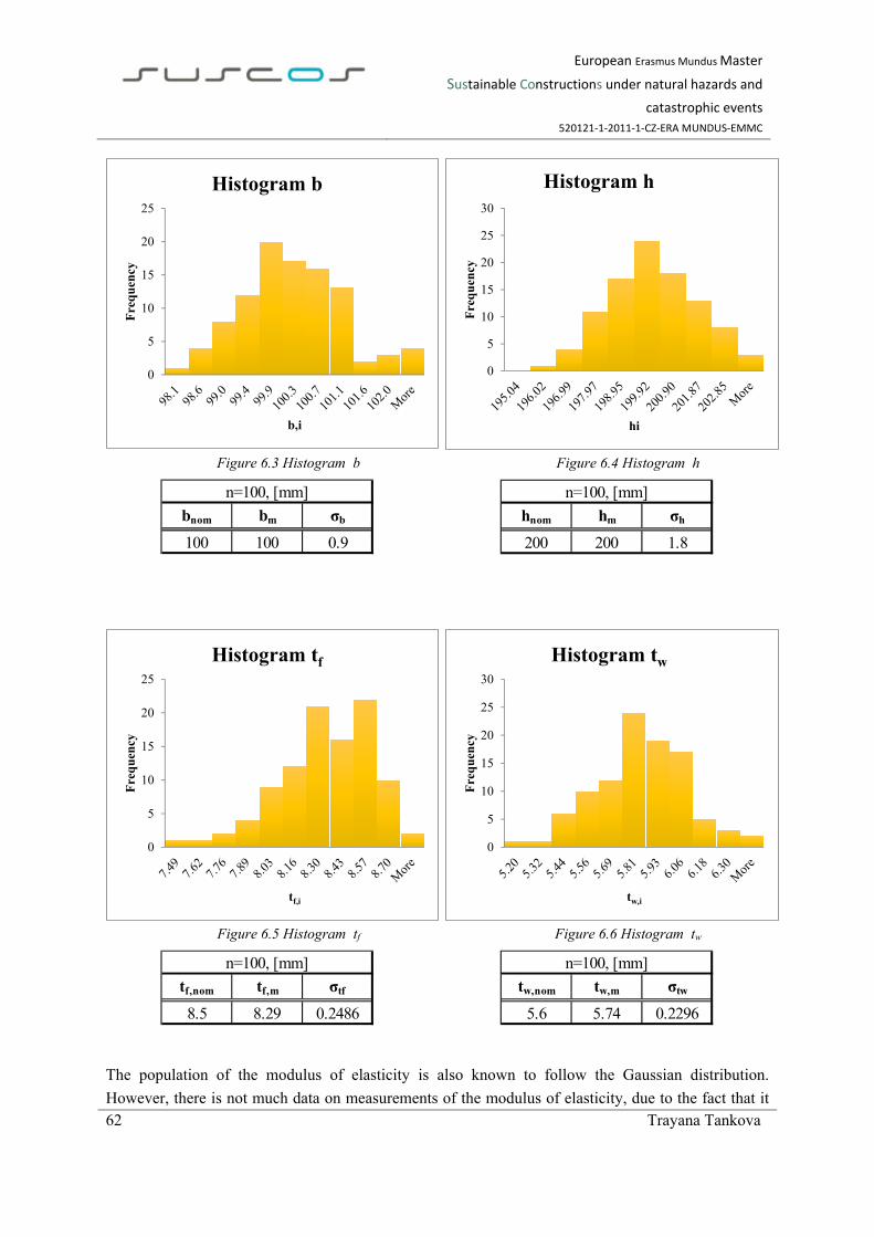
European Erasmus Mundus Master
Sustainable Constructions under natural hazards and
catastrophic events
520121‐1‐2011‐1‐CZ‐ERA MUNDUS‐EMMC
62 Trayana Tankova
Figure 6.3 Histogram b
Figure 6.4 Histogram h
Figure 6.5 Histogram tf
Figure 6.6 Histogram tw
The population of the modulus of elasticity is also known to follow the Gaussian distribution.
However, there is not much data on measurements of the modulus of elasticity, due to the fact that it
0
5
10
15
20
25
Fre
qu
ency
b,i
Histogram b
bnom bm σb
100 100 0.9
n=100, [mm]
0
5
10
15
20
25
30
Fre
qu
ency
hi
Histogram h
hnom hm σh
200 200 1.8
n=100, [mm]
0
5
10
15
20
25
Fre
qu
ency
tf,i
Histogram tf
tf,nom tf,m σtf
8.5 8.29 0.2486
n=100, [mm]
0
5
10
15
20
25
30
Fre
qu
ency
tw,i
Histogram tw
tw,nom tw,m σtw
5.6 5.74 0.2296
n=100, [mm]

European Erasmus Mundus Master
Sustainable Constructions under natural hazards and
catastrophic events
520121‐1‐2011‐1‐CZ‐ERA MUNDUS‐EMMC
Trayana Tankova 63
is very difficult to measure the modulus; moreover, even if the same measurement is considered, two
different people may obtain with very different results. In this example recommendations from [15]
are adopted.
Another property which is difficult to find are the residual stresses. Apparently, their measurement is
very expensive and therefore, there are not many results. Distribution is assumed from [16].
Moreover, this distribution has a mean value which is much lower than the nominal, which is also
favourable.
Finally, for the population of the member imperfection, it is also very difficult to find information,
even though it is being standardized. For this example, the statistical parameters given in [16] are
adopted.
Figure 6.7 Histogram e0/L
Figure 6.8 Histogram residual stresses
6.2 NUMERICAL MODELLING [17]
In order to obtain “experimental” results [17], large number of finite element simulations was carried
out. Using numerical models for experimental results is reported to be useful way of obtaining results
[5], because the output can be monitored, and in case of real experiments sometimes it is not possible
to capture the real behaviour.
In this experimental programme, finite element software product Abaqus 6.12[18] was used. Each
column is modelled with four-node linear shell elements (S4) with six degrees of freedom.
0
5
10
15
20
25
30
Fre
qu
ency
e0/Li
Histogram e0/L
e0/Lnom e0/Lm σe0/L
0.001 0.00085 0.0002
n=100, [-]
0
2
4
6
8
10
12
14
16
18F
req
uen
cy
RS
Histogram RS
RSnom RSm σRS
106.5 71 17.75
n=100, [MPa]

European Erasmus Mundus Master
Sustainable Constructions under natural hazards and
catastrophic events
520121‐1‐2011‐1‐CZ‐ERA MUNDUS‐EMMC
64 Trayana Tankova
Advanced analyses were performed using geometrical and material nonlinearities with imperfections,
also known as GMNIA. This type of analysis allows to capture the second order effects which are
essential for the stability problem.
Material nonlinearity is incorporated in the model by using elastic-plastic constitutive law based on
Von-Misses yield criterion.
Figure 6.9 Finite element model
Geometrical imperfection were modelled using initial sinusoidal imperfection of amplitude
e0=L/1000. The imperfection is introduced in the weak axis of the cross-section.
The load is applied using load stepping routine, in which the increment size is chosen in order to meet
the accuracy and convergence criteria. The equilibrium equations are solved for each increment using
Newton-Raphson iteration technique.
The adopted mesh is 16 sub-divisions in the web and flanges and 100 divisions along the members
axis.
The boundary conditions are implemented as end fork conditions in the shell model. The following
restraints are used - vertical (δy) and transverse (δz) displacements and rotation about xx axis (ϕx) are
prevented at supports. In addition, longitudinal displacement (δx) is prevented in one end. End cross-
sections are modelled to remain straight.

European Erasmus Mundus Master
Sustainable Constructions under natural hazards and
catastrophic events
520121‐1‐2011‐1‐CZ‐ERA MUNDUS‐EMMC
Trayana Tankova 65
6.3 RESULTS AND DISCUSSION
6.3.1 INTRODUCTION
In this section, the results are presented and further discussed based on comparisons between different
approaches and considering different variables. The assessment is performed based on the partial
safety factor γM. Different types of comparisons are used:
Firstly, the influence of each basic variable: all basic variables are modelled separately, and
the other variables are kept with nominal characteristics, in order to compare the impact of
each basic variable on the resistance function;
Secondly, the combinations of random variables are considered; in reality they are always
acting together and their combined impact is being analysed;
Subsequently, the influence of establishing a model using only nominal properties for basic
variables is considered. Their variability is further accounted using the procedure of Annex D;
Finally, the simplified procedures are applied in order to illustrate previously defined trends
in section 5.
The column buckling formulation of EN 1993-1-1 [2] is adopted for resistance function. Based on that
resistance function, partial safety factors are calculated using the procedure proposed in Annex D of
EN 1990. The procedure is applied as shown in Figure 3.5. The theoretical quantities of the resistance
function rt,i are calculated and further analysed with the experimental ones re,i = Nb. The errors terms δi
are then obtained, leading to the coefficient of variation Vδ having three different quantities for each
slenderness respectively. Furthermore, the sensitivity of the resistance function to the basic input
variables is studied. Since the resistance function is a complex function, then the computation of the
coefficient of variation Vrt involves partial derivatives of the resistance function at each variable. The
partial derivatives are computed numerically using expression 6.1 and very small values of “Xi” for
each test specimen separately, leading to a scatter of γM,i for each specimen.
i
jitjiit
i
t
X
XXXrXXXXr
X
r
),....,...,(),....,...,( 11
(6.1)
Finally, the mean value of γM for each slenderness range is obtained and further compared in the cases
listed above.
In this section, if it is not otherwise specified, the method which is used to obtain the partial safety
factor is the procedure of Annex D using the partial derivatives.
The simplified procedures are applied as proposed in section 4.
6.3.2 INFLUENCE OF EACH BASIC VARIABLE
The influence of each basic variable is considered as each of them is modelled separately as a random
variable and the remaining properties are kept with nominal characteristics. Furthermore, the
procedure of Annex D is applied using the partial derivatives only at the respective variable and

European Erasmus Mundus Master
Sustainable Constructions under natural hazards and
catastrophic events
520121‐1‐2011‐1‐CZ‐ERA MUNDUS‐EMMC
66 Trayana Tankova
partial safety factors γM,i are calculated for each column. Finally, the mean value of each slenderness
case is obtained and further plotted in Figure 6.10 .
Observing Figure 6.10, the favourable effect of the yield stress distribution is clear. Through all
slenderness ranges, the partial safety factors are always lower than unity and more or less
homogeneous.
On the contrary, if the modulus of elasticity is considered as only variable, it is almost in every case
presenting with partial safety factors which are higher than one. This issue can be addressed to the
fact that the mean value of the distribution is considered equal to the nominal one, and therefore there
is range in which the modulus has lower quantity than the nominal. Hence the partial safety factor
should “compensate” for those lower values. It is can be noticed that within low-to-intermediate
slenderness range, the partial safety factors are lower since in that range it is has minor influence on
the stability problem (see =0.3 and 0.6). However, in the medium-to-high slenderness range partial
safety factors of 1.1 are observed.
Figure 6.10 Mean value of partial safety factor for each variable
Similarly to the modulus of elasticity, the geometrical properties have mean value around the nominal
value and therefore the partial safety factors are accounting for that by resulting in higher values.
Unlike the modulus of elasticity, the geometrical properties exhibit more or less the same partial
safety factor through all slenderness cases, due to fact that they are entering the resistance function
both through the area and the moment of inertia. As the area is more important in the low-to-
intermediate slenderness range, the inertia has more influence in the high slenderness range.
When considering the imperfection, their influence is only accounted through the difference of
experimental value when compared to the nominal value, because they are incorporated in the design
0.5
0.6
0.7
0.8
0.9
1
1.1
1.2
0.3 0.6 1 1.4 1.8 2.2
γ M
Slenderness, λnom
fy E CS RS GI

European Erasmus Mundus Master
Sustainable Constructions under natural hazards and
catastrophic events
520121‐1‐2011‐1‐CZ‐ERA MUNDUS‐EMMC
Trayana Tankova 67
model of EN 1993-1-1 and they are not explicitly considered in the resistance function and therefore,
it is not possible to obtain coefficient of variation Vrt when they are considered as a random variables.
As the residual stresses have a mean value lower than the nominal, the favourable effect, indeed, is
seen by partial safety factors lower than unity. The geometrical imperfection however is presenting
partial safety factor higher than unity in the intermediate slenderness range, where it actually cannot
be neglected.
Further comparison of the imperfections is presented in Figure 6.11, where two additional cases are
considered, namely: i) imperfections action together; ii) residual stresses changing according the
change of the yield stress. Influence of modelling with residual stresses as a function of the nominal
or the actual yield stress is found negligible. On the other hand, when both imperfection types are
combined, for intermediate slenderness values, differences between both residual stresses and
geometrical imperfection modelled separately, are found.
Figure 6.11 Mean value of partial safety factor for each variable
In reality, it is not possible to distinguish between basic variables. Since their nature is random, the
basic variables act together and it is not possible to isolate them. However, it was useful for better
understanding to try to quantify the influence of each variable.
6.3.3 COMBINATIONS OF BASIC VARIABLES
The combinations of variables are chosen as each of them is modelled separately with the random
variables considered and the remaining properties are kept with nominal characteristics, similarly to
the previous section. Furthermore, the procedure of Annex D is applied using the partial derivatives
0.5
0.6
0.7
0.8
0.9
1
1.1
0.3 0.6 1 1.4 1.8 2.2
γ M
Slenderness, λnom
fy fy+RS(fy) RS+GI RS GI

European Erasmus Mundus Master
Sustainable Constructions under natural hazards and
catastrophic events
520121‐1‐2011‐1‐CZ‐ERA MUNDUS‐EMMC
68 Trayana Tankova
only at the respective variables and partial safety factors γM,i are calculated for each column. Finally,
the mean value of each slenderness case is obtained and further plotted in Figure 6.12.
The following combinations of variables are considered:
Yield stress and cross-section properties (fy+CS) – this combination it is aimed at evaluating
the influence of the variability of the cross-section relatively to the yield stress. The partial
derivatives of the geometrical properties are performed with respect to the area and moment
of inertia;
Yield stress and modulus of elasticity (fy+E) – similarly to the previous combination, here the
impact of the Young’s modulus relatively to the yield stress is evaluated;
Yield stress, cross-section properties and modulus of elasticity (fy+CS+E) – finally all the
basic variables which are considered explicitly in the formulation of the EN 1993-1-1 are
combined in order to obtain a realistic value of the partial safety factor;
Yield stress, cross-section properties and modulus of elasticity; geometrical imperfection and
residual stresses (fy+CS+E+GI+RS) – this combination is compared with the previous in
order to see the influence;
Figure 6.12 summarizes the partial safety factors for the various slenderness ranges considered. In all
cases the partial safety factors obtained considering the yield stress as the only variable is added.
Figure 6.12 Combination of variables
In the previous sections, it was already mentioned that the distribution of the yield stress possesses
useful features. Here, it can be observed that it is not valid only when the yield stress is considered as
only variable. When comparing the results for fy+E and fy+CS it is seen that in the low and
intermediate slenderness range fy manages to cover for the variability of the area and modulus of
elasticity. However, in the high slenderness this is not true anymore since the modulus of elasticity
0.5
0.6
0.7
0.8
0.9
1
1.1
1.2
0.3 0.6 1 1.4 1.8 2.2
γ M
Slenderness, λnom
fy fy+CS fy+E fy+CS+E fy+CS+E+RS+GI

European Erasmus Mundus Master
Sustainable Constructions under natural hazards and
catastrophic events
520121‐1‐2011‐1‐CZ‐ERA MUNDUS‐EMMC
Trayana Tankova 69
and the inertia of the cross-section become more influential due to the second order effects. The same
trend is observed when all variables are combined.
It can be also noticed that for =1.4, 1.8 and 2.2, the partial safety factor should be higher than unity,
which is not the case in the present version of EN 1993-1-1[2]. This result is explained by already
mentioned importance of the modulus of elasticity and inertia in the high-slenderness range. In
addition, in the calibration of the buckling curves [16], the scatter of the modulus of elasticity and
moment of inertia was not considered which in turn leads to the observed differences.
6.3.4 INFLUENCE OF MODELLING WITH NOMINAL PARAMETERS
A useful feature is the possibility to model the element with nominal properties and further apply the
procedure of Annex D with the variability of the basic variables, it would be very useful , since it
would reduce significantly the number of finite element simulations. In such case, the partial
derivatives of the resistance function are performed at the nominal value of each basic variable.
Modelling with nominal properties would mean that the coefficient of variation Vδ, which is obtained
from the differences between the numerical and theoretical results is the same regardless of the input
variables. Moreover, it means that epistemic uncertainty is constant for the various slenderness cases,
which in turn is not the reality. In Figure 6.13 it is noticed that the differences between the
experimental and theoretical estimations for the reduction factor χ are not constant thorough the
buckling curve, therefore the model uncertainty differs for every slenderness.
In order to reduce the error between different slenderness ranges, for the vicinity of each slenderness
case in this example, additional simulations are performed in order to obtain the coefficient of
variation of the model Vδ, because if all are considered together the scatter would be higher and it
would lead to a single γM factor.

European Erasmus Mundus Master
Sustainable Constructions under natural hazards and
catastrophic events
520121‐1‐2011‐1‐CZ‐ERA MUNDUS‐EMMC
70 Trayana Tankova
Figure 6.13 Nominal experimental and nominal theoretical
Several combinations are considered as it can be seen from Figure 6.14 to Figure 6.17, the application
of the assumption that the models are built with nominal characteristics and the influence of the
variability is further considered in the application on the procedure of Annex D, leads to safe results.
However, the differences are not constant throughout the different slenderness case as it was
expected.
Figure 6.14 Fy vs (Fy)nom
Table 6.2 fy vs (fy)nom
0.1
0.2
0.3
0.4
0.5
0.6
0.7
0.8
0.9
1
0.2 0.3 0.4 0.5 0.6 0.7 0.8 0.9 1 1.1 1.2 1.3 1.4 1.5 1.6 1.7 1.8 1.9 2 2.1 2.2 2.3 2.4 2.5
χ nom
Slenderness, λnom
Experimental
Theoretical
0.5
0.6
0.7
0.8
0.9
1
1.1
1.2
0.3 0.6 1 1.4 1.8 2.2
γ M
Slenderness, λnom
fy (fy)nom
fy (fy)nom Error
λ=0.3 0.9135 0.9326 2.09%λ=0.6 0.9024 0.9422 4.41%λ=1.0 0.8992 0.9738 8.30%λ=1.4 0.9123 0.9590 5.12%λ=1.8 0.9292 0.9549 2.77%λ=2.2 0.9423 0.9582 1.68%

European Erasmus Mundus Master
Sustainable Constructions under natural hazards and
catastrophic events
520121‐1‐2011‐1‐CZ‐ERA MUNDUS‐EMMC
Trayana Tankova 71
Figure 6.15 Fy+CS vs (Fy+CS)nom
Table 6.3 fy+CS vs (fy+CS)nom
Figure 6.16 Fy+E vs (Fy+E)nom
Table 6.4 fy+E vs (fy+E)nom
0.5
0.6
0.7
0.8
0.9
1
1.1
1.2
0.3 0.6 1 1.4 1.8 2.2
γ M
Slenderness, λnom
fy+CS (fy+CS)nom
fy+CS (fy+CS)nom Error
λ=0.3 0.9309 0.9477 1.80%λ=0.6 0.9187 0.9621 4.73%λ=1.0 0.9517 1.0155 6.70%λ=1.4 1.0058 1.0360 3.01%λ=1.8 1.0427 1.0572 1.39%λ=2.2 1.0638 1.0741 0.97%
0.5
0.6
0.7
0.8
0.9
1
1.1
1.2
0.3 0.6 1 1.4 1.8 2.2
γ M
Slenderness, λnom
fy+E (fy+E)nom
fy+E (fy+E)nom Error
λ=0.3 0.9136 0.9328 2.10%λ=0.6 0.9069 0.9448 4.19%λ=1.0 0.9483 1.0014 5.60%λ=1.4 1.0068 1.0329 2.59%λ=1.8 1.0455 1.0587 1.27%λ=2.2 1.0667 1.0772 0.99%

European Erasmus Mundus Master
Sustainable Constructions under natural hazards and
catastrophic events
520121‐1‐2011‐1‐CZ‐ERA MUNDUS‐EMMC
72 Trayana Tankova
Figure 6.17 Fy +CS+E vs (Fy+CS+E)nom
Table 6.5 fy +CS+E vs
(fy+CS+E)nom
6.3.5 INFLUENCE OF GEOMETRICAL PARAMETERS
In previous sections the partial derivatives for the cross-section properties were performed with
respect to area and moment of inertia. In this section, the influence of performing the derivatives at
each cross-section parameters or as more global – area and moment of inertia is considered. Figure
6.18 summarizes the partial safety factors obtained both alternatives, moreover, it presents the same
comparison based on models with nominal properties. Very small differences are observed and
therefore, the assumption is considered as valid.
Figure 6.18A+I vs. b+h+tf+tw
Additionally, the influence of area and inertia separately is studied. The results comply with the
discussion previously carried out – that the area has more influence in the low-to-intermediate
slenderness, as the inertia in the intermediate-to-high. It is also observed that neglecting the inertia can
0.5
0.6
0.7
0.8
0.9
1
1.1
1.2
0.3 0.6 1 1.4 1.8 2.2
γ M
Slenderness, λnom
fy+CS+E fy+CS+E+RS+GI (fy+CS+E)nom
fy+CS+E (fy+CS+E)nom Error
λ=0.3 0.9312 0.9479 1.79%λ=0.6 0.9231 0.9647 4.51%λ=1.0 0.9914 1.0394 4.84%λ=1.4 1.0672 1.0901 2.15%λ=1.8 1.1131 1.1255 1.12%λ=2.2 1.1387 1.1488 0.89%
0.5
0.6
0.7
0.8
0.9
1
1.1
1.2
0.3 0.6 1 1.4 1.8 2.2
γ M
Slenderness, λnom
CS(A+I) CS(A+I)nom
CS(b+h+tf+tw) CS(b+h+tf+tw)nom

European Erasmus Mundus Master
Sustainable Constructions under natural hazards and
catastrophic events
520121‐1‐2011‐1‐CZ‐ERA MUNDUS‐EMMC
Trayana Tankova 73
lead to high differences. Moreover, the difference remains more or less constant no matter if the
variable is combined with the yield stress or not.
Figure 6.19Influence of cross-section area and inertia
Table 6.6 Influence of area
Table 6.7 Influence of inertia
Figure 6.20Influence of cross-section area and inertia
Table 6.8 Influence of area
Table 6.9Influence of inertia
6.3.6 SIMPLIFIED PROCEDURES
The simplified procedures are applied in the context presented in previous sections.
0.5
0.6
0.7
0.8
0.9
1
1.1
1.2
0.3 0.6 1 1.4 1.8 2.2
γ M
Slenderness, λnom
CS(A+I)nom CS(A)nom CS(I)nom CS(A+I)nom CS(A)nom Errorλ=0.3 1.0844 1.0769 -0.696%λ=0.6 1.0668 1.0508 -1.50%λ=1.0 1.0814 1.0250 -5.21%λ=1.4 1.0802 0.9808 -9.20%λ=1.8 1.0880 0.9670 -11.12%λ=2.2 1.0974 0.9670 -11.88%
CS(A+I)nom CS(I)nom Errorλ=0.3 1.0844 1.0333 -4.712%λ=0.6 1.0668 1.0169 -4.68%λ=1.0 1.0814 1.0536 -2.57%λ=1.4 1.0802 1.0547 -2.36%λ=1.8 1.0880 1.0611 -2.48%λ=2.2 1.0974 1.0694 -2.55%
0.5
0.6
0.7
0.8
0.9
1
1.1
1.2
0.3 0.6 1 1.4 1.8 2.2
γ M
Slenderness, λnom
(fy+CS)nom fy+CS(A)nom fy+CS(I)nom
(fy+CS)nom fy+CS(A)nom Error
λ=0.3 0.9477 0.9405 -0.763%λ=0.6 0.9621 0.9494 -1.33%λ=1.0 1.0155 0.9785 -3.64%λ=1.4 1.0360 0.9614 -7.21%λ=1.8 1.0572 0.9563 -9.55%λ=2.2 1.0741 0.9591 -10.70%
(fy+CS)nom fy+CS(I)nom Errorλ=0.3 0.9477 0.9327 -1.585%λ=0.6 0.9621 0.9438 -1.90%λ=1.0 1.0155 0.9918 -2.33%λ=1.4 1.0360 1.0106 -2.46%λ=1.8 1.0572 1.0304 -2.54%λ=2.2 1.0741 1.0463 -2.59%

European Erasmus Mundus Master
Sustainable Constructions under natural hazards and
catastrophic events
520121‐1‐2011‐1‐CZ‐ERA MUNDUS‐EMMC
74 Trayana Tankova
1) P1 (fy) – as it was presented in section 4.3, it is based on expression (3.9) and only the
variability of the yield stress is taken into account. As a result, from the fact that the mean
and standard deviation of the yield strength are represented by single values, global partial
safety coefficients γM are obtained for each slenderness range.Figure 6.21 and Table 6.10
summarize the results obtained with this procedure.
In addition, Figure 6.21 and Table 6.10 present results for the procedure in f) using the
partial derivatives only for fy, it is “acting as if” the yield strength is the only variable.
Nonetheless, the percent difference is computed with regard to (global) fy+CS+E.
Observing Table 6.10, it can be pointed out that P1 provides results which are unsafe when
compared to fy+CS+E.
These results confirm the trends observed in section 5.3. Nevertheless, it should be noticed
that the percentual difference might be different for the same Vδ since the distributions of
the basic variables are different from the ones used in section 5.
Figure 6.21 Comparison of partial safety factors
Table 6.10 Difference P1(fy)
2) P2 (fy+A) – as an extension of the assumptions above, here the geometrical properties are
included are basic variables. P2 is assumed as presented in section 4.4. In this case, the
random variables are the yield strength and the cross-section area. The mean value and
standard deviation of the area are calculated using Eq. (3.23) and Eq. (3.24). Similarly to
P1, single results for the partial safety coefficient γM are obtained. Figure 6.22 and Table
6.11summarize the results obtained with this alternative;
It is noticed for =2.2, the procedure starts to become unsafe, unlike the observations in
section 5, where the procedure was showing only safe-sided results. However, this “misfit”
is explained by the fact that the distribution in this example has much lower coefficient of
variation for the area ~2.3%, instead of 4% which were used in section 5.
0.5
0.6
0.7
0.8
0.9
1
1.1
1.2
0.3 0.6 1 1.4 1.8 2.2
γ M
Slenderness, λnom
fy+CS+E fy P1(fy)
fy+CS+E fy P1 (fy) Error
λ=0.3 0.9312 0.9135 0.9237 -0.81%λ=0.6 0.9231 0.9024 0.9376 1.57%λ=1.0 0.9914 0.8992 0.9939 0.26%λ=1.4 1.0672 0.9123 1.0430 -2.26%λ=1.8 1.1131 0.9292 1.0745 -3.46%λ=2.2 1.1387 0.9423 1.0932 -4.00%

European Erasmus Mundus Master
Sustainable Constructions under natural hazards and
catastrophic events
520121‐1‐2011‐1‐CZ‐ERA MUNDUS‐EMMC
Trayana Tankova 75
Figure 6.22 Comparison of partial safety factors
Table 6.11 Difference P2(fy+A)
3) P2 (fy+A+I) – same as 2, but with the additional consideration of the moment of inertia as
a random variable. Correspondingly to P2 (fy+A), the mean value and standard deviation of
the moment of inertia are calculated using Eq. (3.23) and Eq. (3.24). Here also single
results for the partial safety coefficient γM are obtained. Figure 6.23 and Table 6.12
summarize the results obtained with this alternative;
Moreover, Figure 6.23 and Table 6.12 present results for the procedure in fy+CS using the
partial derivatives in case that the yield strength, column cross-section dimensions are the
basic variables and the variability of the Young’s modulus is neglected. However, the
percent difference is evaluated with regard to fy+CS+E.
Comparing Table 6.11 and Table 6.12, it can be observed, that P2 (fy+A) and P2 (fy+A+I)
provide results which are on the safe side when associated to fy+CS+E. However, this
difference increases with increased number of variables.
0.5
0.6
0.7
0.8
0.9
1
1.1
1.2
0.3 0.6 1 1.4 1.8 2.2
γ M
Slenderness, λnom
fy+CS+E fy+CS P2(fy+A)
fy+CS+E fy+CSP2
(fy+A)Error
λ=0.3 0.9312 0.9309 0.9423 1.19%λ=0.6 0.9231 0.9187 0.9562 3.58%λ=1.0 0.9914 0.9517 1.0270 3.59%λ=1.4 1.0672 1.0058 1.0826 1.44%λ=1.8 1.1131 1.0427 1.1170 0.36%λ=2.2 1.1387 1.0638 1.1364 -0.20%

European Erasmus Mundus Master
Sustainable Constructions under natural hazards and
catastrophic events
520121‐1‐2011‐1‐CZ‐ERA MUNDUS‐EMMC
76 Trayana Tankova
Figure 6.23 Comparison of partial safety factors
Table 6.12Difference P2(fy+A+I)
4) P2 (fy+A+I+E) – finally variability of yield stress, Young’s modulus and cross-sectional properties are grouped together using P2. Results are presented in Figure 6.24and Table 6.13.
Figure 6.24 Comparison of partial safety factors
Table 6.13 Difference P2(fy+A+I+E)
The example confirms the trends shown in section 5.3. However, it should be noted that it is not
possible to directly compare results since the distributions used in sections 5.3 and 6 have different
parameters – ratio between mean and nominal values, standard deviation. Despite that fact, the trends
drawn in section 5 for the simplified procedures are confirmed with the example in chapter 6.
0.5
0.6
0.7
0.8
0.9
1
1.1
1.2
0.3 0.6 1 1.4 1.8 2.2
γ M
Slenderness, λnom
fy+CS+E fy+CS P2(fy+A+I)
fy+CS+E fy+CSP2
(fy+A+I)Error
λ=0.3 0.9312 0.9309 0.9791 5.15%λ=0.6 0.9231 0.9187 0.9934 7.61%λ=1.0 0.9914 0.9517 1.0666 7.59%λ=1.4 1.0672 1.0058 1.1248 5.40%λ=1.8 1.1131 1.0427 1.1607 4.28%λ=2.2 1.1387 1.0638 1.1808 3.70%
0.5
0.6
0.7
0.8
0.9
1
1.1
1.2
0.3 0.6 1 1.4 1.8 2.2
γ M
Slenderness, λnom
fy+CS+E P2(fy+A+I+E)
fy+CS+E Error
λ=0.3 0.9312 10.41%λ=0.6 0.9231 13.00%λ=1.0 0.9914 13.11%λ=1.4 1.0672 10.70%λ=1.8 1.1131 9.52%λ=2.2 1.1387 8.94%1.2405
P2(fy+A+I+E)
1.02811.04311.12131.18141.2190

European Erasmus Mundus Master
Sustainable Constructions under natural hazards and
catastrophic events
520121‐1‐2011‐1‐CZ‐ERA MUNDUS‐EMMC
Trayana Tankova 77
7 BRIEF ANALYSIS OF THE STATISTICAL DEPENDENCY BETWEEN
BASIC VARIABLES
Throughout the previous chapters, there was always the same assumption which in fact is the
assumption adopted in EN 1990, i.e., the basic variables are treated as statistically independent.
However, it is not always the case. For example, the yield stress is dependent on the plate thickness;
or the cross-section dimensions are dependent to each other due to the fact that the element mass is
strictly monitored, the modulus of elasticity and the elastic strain, etc.
It was already explained that it is very hard to obtain information about the distributions of the basic
variables. Therefore, it is even more difficult to obtain the magnitude of the correlation between basic
variables. However, it is worth to try to quantify the impact of the correlation, i.e. if it is safe-sided
(within certain reasonable limits) to neglect it.
In this chapter, the statistical dependence of the yield stress and thickness of the plate is treated. It is a
negative correlation, i.e. when one parameter is increasing, the other is decreasing.
7.1 CORRELATION BASED ON EXPERIMENTS
In [19], a large number (689) of tests was performed on yield stress and geometrical properties. Based
on that data, an attempt to estimate the correlation coefficient is performed. As the yield stress is
dependent on the plate thickness, firstly the scatter of flange thickness and yield stress is considered.
689 tests from [19] on S235 steel are considered for this analysis. The geometrical properties were
measured on both H and I sections, namely IPE80, IPE120, IPE 140, IPE 140, IPE 160, IPE 180, IPE
240, IPE 270, HEB 100, HEB 140, HEB 180. Although all flange thicknesses are smaller than 16mm,
a certain trend can be seen when observing the scatter on Figure 7.1.
Figure 7.1 Correlation between yield stress and flange thickness
0
50
100
150
200
250
300
350
400
450
0 5 10 15
f y[M
Pa]
tf [mm]

European Erasmus Mundus Master
Sustainable Constructions under natural hazards and
catastrophic events
520121‐1‐2011‐1‐CZ‐ERA MUNDUS‐EMMC
78 Trayana Tankova
The correlation coefficient is obtained based on expression (2.25), and the value of ρ = -0.611 is
found. Figure 7.1 clearly shows the negative correlation between the variables, yet it is confirmed by
the calculation.
Additionally, the correlation between the cross-section area and yield stress is studied and correlation
coefficient is found equal to -0.681, similarly to the one above. The scatter is shown in Figure 7.2.
Figure 7.2 Correlation between yield stress and cross-section area
7.2 IMPLEMENTATION OF THE CORRELATION
The correlation between basic input variables in a function was discussed in sections 2.6 and 2.7.
There it can be seen that the statistical dependence of the variables has no impact on the mean value
of the function, however additional cross terms appear in the variance of the function, i.e. in the error
propagation. On the other hand, the procedure adopted in Annex D of EN 1990 that was presented in
section 3.3, considers statistical independence of the basic input variables and therefore, the
coefficient of variation Vrt is calculated using expression (2.29), obtained from expression (2.28).
Here, in order to account for the correlation between basic variables, expression (2.28) and the
coefficient of variation Vrt becomes:
j
n
ji
n
ji iXXji
k
jj
j
j
m
rt X
g
X
g
X
Xg
XgV
ji1,
,
2
12
2 1 (7.1)
The remaining part of the procedure remains unchanged.
0
50
100
150
200
250
300
350
400
450
0 10 20 30 40 50 60 70
f y[M
Pa]
A, [cm2]

European Erasmus Mundus Master
Sustainable Constructions under natural hazards and
catastrophic events
520121‐1‐2011‐1‐CZ‐ERA MUNDUS‐EMMC
Trayana Tankova 79
In order to consider the correlation in terms of difference between partial safety factors, the samples in
section 5.2 are used and the comparison is performed using the same assumptions as in section 5.3.1
as here a correlation between area and yield stress is assumed. Moreover, the correlation coefficient is
assumed equal to -0.681 as calculated for the experimental results in the previous section.
Additionally, assumption for the coefficient of variation Vδ was also made.
Figure 7.3 summarizes the results. It was found that higher difference between considering the
correlation or not is found for Vδ=0. The maximum observed difference is 3.6%, meaning that
including the covariance would result in 3.6% lower partial safety factors. Therefore, neglecting the
correlation is actually safe-sided and the simplification does not lead to high differences.
Figure 7.3 Correlation coefficient -0.681
Additionally, an extreme case of -1.0 is also considered. Here the same assumption for Vδ=0, leads to
5.6% difference, which is also safe-sided.
1
1.05
1.1
1.15
1.2
1.25
0 0.5 1 1.5 2 2.5
1/ex
p(-k
d,nQ
-0,5
Q2 )
Slenderness, λnom
AnnexD(fy+A)
Mean(fy+A)
AnnexD(fy+A+fyA)
Mean(fy+A+fyA)
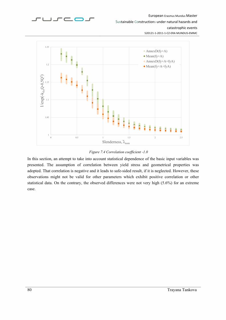
European Erasmus Mundus Master
Sustainable Constructions under natural hazards and
catastrophic events
520121‐1‐2011‐1‐CZ‐ERA MUNDUS‐EMMC
80 Trayana Tankova
Figure 7.4 Correlation coefficient -1.0
In this section, an attempt to take into account statistical dependence of the basic input variables was
presented. The assumption of correlation between yield stress and geometrical properties was
adopted. That correlation is negative and it leads to safe-sided result, if it is neglected. However, these
observations might not be valid for other parameters which exhibit positive correlation or other
statistical data. On the contrary, the observed differences were not very high (5.6%) for an extreme
case.
1
1.05
1.1
1.15
1.2
1.25
0 0.5 1 1.5 2 2.5
1/ex
p(-k
d,nQ
-0,5
Q2 )
Slenderness, λnom
AnnexD(fy+A)
Mean(fy+A)
AnnexD(fy+A+fyA)
Mean(fy+A+fyA)

European Erasmus Mundus Master
Sustainable Constructions under natural hazards and
catastrophic events
520121‐1‐2011‐1‐CZ‐ERA MUNDUS‐EMMC
Trayana Tankova 81
8 CONCLUSIONS AND FUTURE RESEARCH
8.1 CONCLUSIONS
This study summarized different possibilities for the safety assessment of design rules focusing on the
buckling resistance of steel members. The various simplifications were explained and assessed based
on assumed distributions for the basic variables. Different basic variables were considered, including:
i) material properties; ii) geometrical properties. Moreover, the influence of each basic variable was
studied in the numerical example in section 6.
It was shown that simplified procedures which include the variability of the yield strength as the only
basic variable may be unsafe for certain slenderness ranges when compared to the Annex D procedure
considering all relevant basic input variables.
When geometrical properties were included, P2 always showed results on the safe side. However, a
clear trend of increasing the error between P2 and the “full” Annex D with increased number of
variables considered was noted in both the numerical validation of chapter 5 and the example
presented in chapter 6. This results from the simplified procedure simply adding the variability of the
input variables, while the Annex D procedure using the partial derivatives for Vrt, accounts for the
function and each variable gives its contribution according to its contribution in the resistance
function, at the respective slenderness value. In other words, the simplified procedures inevitably
calculate a “too large” value of Vrt.
Additionally, it is noticed that the difference between the “full Annex D” and the simplified procedure
for each slenderness range become more homogeneous with an increased number of basic random
variables. This tendency can be seen as very useful in case of adopting adjustment function or factors
for the simplified procedures, as proposed in [14].
Moreover, the influence of each variable was discussed based on the numerical example in section 6.
It was shown that the distribution of the yield stress has favourable effect on the partial safety factor
γM i.e. it reduces its value. On the contrary, the distributions of the geometrical properties and
Young’s modulus lead to higher partial safety factors. It was observed that when the basic variables
are combined, the yield stress may compensate for the distributions of geometry and modulus of
elasticity. However, in the high slenderness range, the favourable effect was not enough due to the
higher importance of the stiffness parameters.
A try to assess the partial safety factors based on models with nominal properties was also presented.
It was shown that the differences are small, nevertheless not constant. Keeping in mind those
observations, it is not possible to conclude that models with nominal properties can be used for safety
assessment.
Additionally, the scatter of member imperfection and residual stresses was also included in the
numerical models. Imperfections, being basic variables incorporated in the design procedure, are

European Erasmus Mundus Master
Sustainable Constructions under natural hazards and
catastrophic events
520121‐1‐2011‐1‐CZ‐ERA MUNDUS‐EMMC
82 Trayana Tankova
difficult to assess explicitly, therefore their impact was only accounted in the coefficient of variation
of the model Vδ.
Although all the numerical comparisons were performed only on the basis of the flexural buckling of
columns, the conclusions should be equally valid to other stability phenomena (LTB of beams, TB
and LTB of columns and the buckling resistance of beam-columns). These other stability problems
will be addressed in the near future to confirm this.
In EN 1990 and in the simplified procedures, the same assumption was adopted – the basic variables
are statistically independent. In chapter 7, an attempt to consider correlation between basic variables
was proposed. The correlation between yield stress and plate thickness was only accounted for. In
order to evaluate reasonable correlation coefficient, statistical data from real experiments was used. It
was shown that if the statistical dependence is neglected, the differences are not very high and the
result is safe sided, for the case considered. However, different results may be observed when other
basic variables are used. Therefore, the topic should be further explored.
8.2 FUTURE RESEARCH
The scope of this study has certain limitations and therefore it should be further extended in the
following directions:
Here, the safety assessment was performed based only on the flexural buckling of columns, as
already mentioned it is expected that the conclusions made would be equally valid for other
stability modes, however it is worth to extend the study for LTB of beams, TB and LTB of
columns and the buckling resistance of beam-columns in order to confirm the same trend.
Furthermore, the concept should be tested for other failure modes such as ductile and brittle
failure modes.
In chapter 6, it was discussed that many parameters lack sufficient statistical characterization.
Consequently, it would be very useful, if such data can be collected. In order to achieve that, a
European database is developed under SAFEBRICTILE project. It can provide the needed
statistical characterization and allow to give guidance to the designers and researchers on
which basic variables should be considered;
The safety assessment procedure should be developed, in order to provide clear guidance to
designers and researchers on how to assess new design rules. In addition, a guidance on which
basic variables are relevant for the different failure modes is also required;
Finally, and attempt to include statistical dependence was presented, however it was only
focused on correlation between plate thickness and yield stress. As already mentioned, it
would be useful to extend the study to correlation between other basic variables and check if
it is safe-sided to assume statistical independence of the relevant basic variables.

European Erasmus Mundus Master
Sustainable Constructions under natural hazards and
catastrophic events
520121‐1‐2011‐1‐CZ‐ERA MUNDUS‐EMMC
Trayana Tankova 83
REFERENCES
[1] Eurocode (2002) – EN 1990, Eurocode – Basis of structural design, CEN, Brussels;
[2] Eurocode (2005) – EN 1993-1-1, Eurocode 3: Design of steel structures - Part 1-1:
General rules and rules for buildings CEN, Brussels;
[3] Ang, A.H-S., Tang, W.H., Probability Concepts in Engineering. Emphasis on Applications to
Civil and Environmental Engineering, 2nd edition, Wiley (2007);
[4] Snedecor, G.W., Cochran, W.G., Statistical methods, 8th edition, Blackwell (1989);
[5] Joint Committee on Structural Safety (2001), Probabilistic Model Code, Parts 1 to 3;
[6] Vrouwenvelder, A.C.W.M., (2002), Developments towards full probabilistic design codes,
Structural safety, 24, pp. 417- 432
[7] Taras, A., Simões da Silva, L. (2012) ECCS – TC8 TC8-2012-06-xxx European
Recommendations for the Safety Assessment of Stability Design Rules for Steel Structures
[8] Gulvanessian, H., Calgaro, J-A., Holicky, M. Designers’ Guide to EN 1990. Eurocode: Basis of
Design
[9] Rebelo, C., Lopes, N., Simões da Silva, L., Nethercot D., Vila Real, P.M.M. (2009), Statistical
Evaluation of the Lateral-Torsional Buckling Resistance of Steel I-beams, Part 1: Variability of the
Eurocode 3 resistance model, J. of Const. Steel Res., 65, pp. 818-831.
[10] Simões da Silva, L., Rebelo C., Nethercot D. Marques, L., Simões, R., Vila Real, P.M.M. (2009),
Statistical Evaluation of the Lateral-Torsional Buckling Resistance of Steel I-beams, Part 2:
Variability of steel properties, J. of Const. Steel Res., 65, pp. 832-849.
[11] Sedlacek, G., Muller, C. (2006), The European standard family and its basis, J. of Const. Steel
Res., 62, pp. 1047-1059.
[12] Muller, C. (2003), Zum Nachweis ebener Tragwerke aus Stahl gegen seitliches Ausweichen, PhD
Dissertation, Schriftenreihe Stahlbau - RWTH Aachen
[13] Cajot, L.G., Haller, M., Conan, Y., Sedlacek, G., Kraus, O., Rondal, J., Cerfontaine, F.,
Lagerqvist, O., Johansson, B. (2005) Probabilistic quantification of safety of a steel structure
highlighting the potential of steel versus other materials;
[14] Taras, A., Simões da Silva, L (2013), Development of a standard safety assessment procedure.
Previous and planned work, RFCS Project SAFEBRICTILE, WP1 Presentation.
[15] DNV (1995), Guideline for Offshore Structural Reliability Analysis – Chapter 7, DNV
Report No. 95-2018, Det Norske Veritas, Hovik, Norway.

European Erasmus Mundus Master
Sustainable Constructions under natural hazards and
catastrophic events
520121‐1‐2011‐1‐CZ‐ERA MUNDUS‐EMMC
84 Trayana Tankova
[16] Strating, J., Vos, H. (1973), Simulation sur Ordinateur de la Coubre C.E.E.M de Flambement á
l‘аide de la Méthode de Monte-Carlo, Construction Métallique, nº2 pp. 23-39
[17] Marques, L. (2012), Tapered Steel Members: Flexural and Lateral-Torsional Buckling, PhD
Dissertation, University of Coimbra
[18] Abaqus (2012). v.6.12, Dassault Systems/Simulia, Providence, RI, USA.
[19] Byfield, M. P., Davies, J. M., Dhanalakshmi, M. (2005), Calculation of strain hardening
behaviour based on mill tests, J. of Const. Steel Res., 61, pp. 133-150.
[20] Rondal,J., Maquoi, R., (1979) Formulations D’Ayrton-Perry pour Le Flambement des Barres
Metalliques Construction Métallique, nº4 pp. 41-53
[21] Beer, H., Schulz, G. (1970), Bases Théoriques des Courbes Européennes de Flambement,
Construction Métallique, n°3, pp. 37-57
[22] Maquoi, R., Rondal, J. (1978), Mise en Équation des Nouvelles Courbes Européennes de
Flambement, Construction Métallique, nº1 pp. 17-30
[23] ECCS Technical Committee 8 (2006), Stability, Rules for Member Stability in EN 1993 -1-1.
Background documentation and design guidelines
[24] Taras, A. (2010), Contribution to the Development of Consistent Stability Design Rules for Steel
Members, PhD Dissertation, Graz University of Technology.


