Comparative assessment of evapotranspiration derived from NCEP and ECMWF global datasets through...

ATMOSPHERIC SCIENCE LETTERSAtmos. Sci. Let. 14: 118–125 (2013)Published online in Wiley Online Library(wileyonlinelibrary.com) DOI: 10.1002/asl2.427

Comparative assessment of evapotranspiration derivedfrom NCEP and ECMWF global datasets throughWeather Research and Forecasting modelPrashant K. Srivastava,*Dawei Han, Miguel A. Rico Ramirez and Tanvir IslamWater and Environment Management Research Centre, Department of Civil Engineering, University of Bristol, UK

*Correspondence to:P. K. Srivastava, Water andEnvironment ManagementResearch Centre, Department ofCivil Engineering, University ofBristol, Bristol, BS8 1TR, UK.E-mail: [email protected]

Received: 14 December 2012Revised: 30 January 2013Accepted: 30 January 2013

AbstractIn many hydro-meteorological applications, it is not always possible to get access to insitu weather measurements, especially for the ungauged catchments. This study exploresthe performances of downscaled weather data for Reference Evapotranspiration (ETo)retrieval using the global European Centre for Medium Range Weather Forecasts (ECMWF)ERA interim and National Centers for Environmental Prediction (NCEP) reanalysis data,simulated through Weather Research and Forecasting (WRF) mesoscale model. The range ofthe Nash-Sutcliffe efficiency calculated for the ECMWF pooled datasets derived ETo variesfrom 0.31 to 0.87, while for NCEP it is found to be 0.11 to 0.38. Bias and Root Mean SquareError (RMSE) are also indicating a very high discrepancy in the NCEP ETo (Bias =−0.05;RMSE = 0.11) as compared to ECMWF (Bias = 0.00; RMSE = 0.06). The overall findingsreveal that ECMWF downscaled products have a much better performance than the NCEP’scounterparts. Copyright 2013 Royal Meteorological Society

Keywords: evapotranspiration; Weather Research and Forecasting model; NCEP;ECMWF; meteorological variables

1. Introduction

Reference Evapotranspiration (ETo) is an impor-tant variable for hydro-meteorological applications(Liguori and Rico-Ramirez, 2013). ETo has significanteffect on catchment water balance and hence wateryield and groundwater recharge (Al-Shrafany et al .,2012) and its reliable estimates from cropped surfacesare required for efficient irrigation management andscheduling (Lorite et al ., 2012). Hence, monitoringETo at local, regional or global scales is important forassessing climate and human-induced effects on natu-ral and agricultural ecosystems (Kustas and Norman,1996; Thakur et al ., 2012). However, to reduce theuncertainty in the ETo estimates, appropriate meteo-rological data selection is important if derived frommesoscale models (Evans et al ., 2011). There arenow choices of global data available for ETo estima-tion with reliable mesoscale model like the WeatherResearch and Forecasting (WRF) model for meteoro-logical applications (Niyogi et al ., 2009; Bromwichet al ., 2009).

Many methods for estimating ETo have been devel-oped, and accurate estimates of ETo are becomingavailable through the use of ground-based observationsusing the Penman Monteith equation (Novak, 2012).But these ground-based observations can cover onlya smaller area. However, larger areas require a largenumber of observation sites because of the heterogene-ity of landscapes and very high variations in the energy

transfer processes (Detto et al ., 2006). Nevertheless,the above-mentioned approaches are very expensiveand labour intensive, so other approaches are requiredsuch as mesoscale models to estimate ETo at largescales. Recently, efforts have been made to determinethe spatial and temporal variability of ETo throughmesoscale model like the MM5 (Ishak et al ., 2010;Niyogi et al ., 2009) but there is a lack of appropriatestudies available with the WRF model, especially fortemperate maritime climate.

There are very rare studies available whichdemonstrated the accuracy of data chosen for theETo estimation from mesoscale model such as WRFusing the global European Centre for Medium RangeWeather Forecasts (ECMWF) ERA interim andNCEP (National Centers for Environmental Predic-tion) reanalysis data to determine the spatial andtemporal distribution of ETo (Buizza et al ., 2005).Therefore hydro-meteorologists would like to knowhow well the downscaled global data products are ascompared to ground-based measurements and whetherit is possible to use the downscaled data for ungaugedcatchments. Even with gauged catchments, most ofthe stations have only rain and flow gauges installed.Measurements of other weather hydro-meteorologicalvariables such as solar radiation, wind speed, airtemperature and dew point are usually missing andthus complicate the problems. Hence, the foremostobjective of this article is to compare the EToproducts estimated from the downscaled ECMWF

Copyright 2013 Royal Meteorological Society

NCEP and ECMWF comparison 119

and NCEP global datasets using the WRF model,centred over the Brue catchment in south west of theEngland. The validations of the products are made byusing the ground-based measurements retrieved frommeteorological weather station located in the Bruecatchment.

2. Materials and methodology

2.1. Study area and datasets

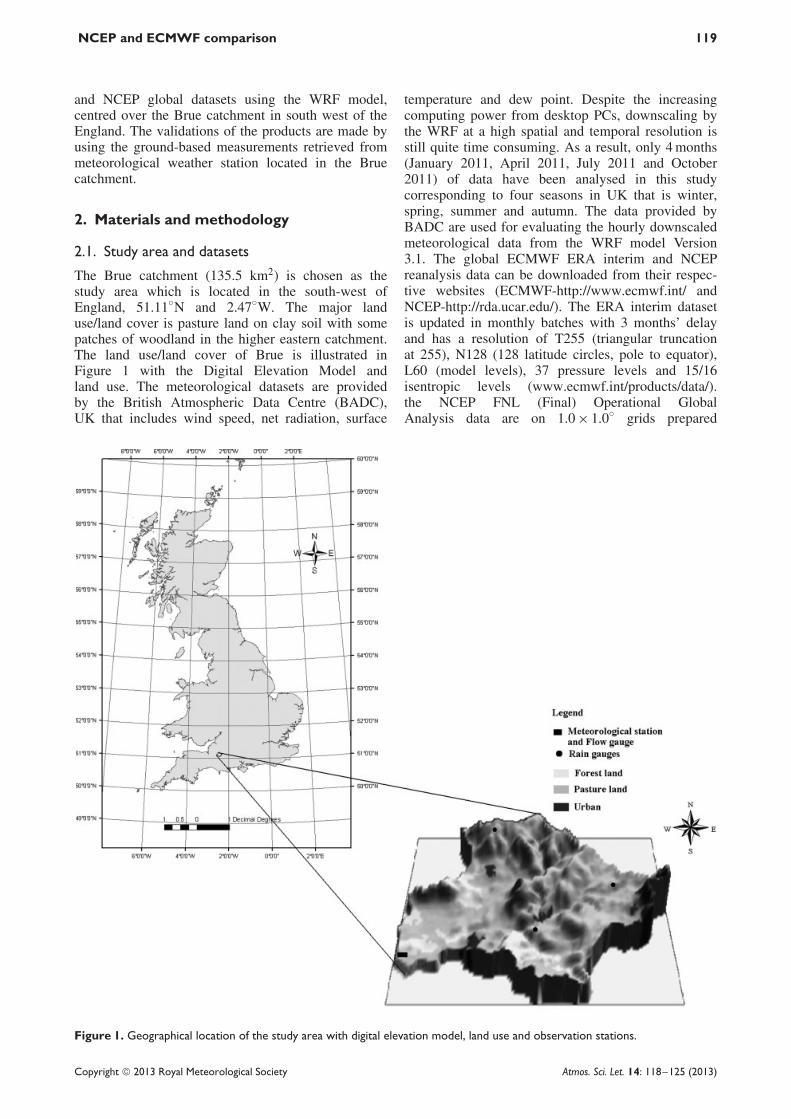
The Brue catchment (135.5 km2) is chosen as thestudy area which is located in the south-west ofEngland, 51.11◦N and 2.47◦W. The major landuse/land cover is pasture land on clay soil with somepatches of woodland in the higher eastern catchment.The land use/land cover of Brue is illustrated inFigure 1 with the Digital Elevation Model andland use. The meteorological datasets are providedby the British Atmospheric Data Centre (BADC),UK that includes wind speed, net radiation, surface

temperature and dew point. Despite the increasingcomputing power from desktop PCs, downscaling bythe WRF at a high spatial and temporal resolution isstill quite time consuming. As a result, only 4 months(January 2011, April 2011, July 2011 and October2011) of data have been analysed in this studycorresponding to four seasons in UK that is winter,spring, summer and autumn. The data provided byBADC are used for evaluating the hourly downscaledmeteorological data from the WRF model Version3.1. The global ECMWF ERA interim and NCEPreanalysis data can be downloaded from their respec-tive websites (ECMWF-http://www.ecmwf.int/ andNCEP-http://rda.ucar.edu/). The ERA interim datasetis updated in monthly batches with 3 months’ delayand has a resolution of T255 (triangular truncationat 255), N128 (128 latitude circles, pole to equator),L60 (model levels), 37 pressure levels and 15/16isentropic levels (www.ecmwf.int/products/data/).the NCEP FNL (Final) Operational GlobalAnalysis data are on 1.0 × 1.0◦ grids prepared

Figure 1. Geographical location of the study area with digital elevation model, land use and observation stations.

Copyright 2013 Royal Meteorological Society Atmos. Sci. Let. 14: 118–125 (2013)

120 P. K. Srivastava et al.

operationally every 6 h. This product is from theGlobal Data Assimilation System, which contin-uously collects observational data. The archivetime series is continuously extended to a near-current date but not maintained in real-time(http://rda.ucar.edu/datasets/ds083.2/). The mainpurposes of these reanalysis data are to delivercompatible, high-resolution and high quality historicalglobal atmospheric datasets for their use in weatherresearch communities.

2.2. Weather Research Forecasting model

The mesoscale model used in this study is the WRFModel with Advanced Research WRF dynamic coreversion 3.1 (Powers, 2007; Schwartz et al ., 2009).WRF is a next-generation, non-hydrostatic, with ter-rain following eta-coordinate mesoscale modellingsystem designed to serve both operational forecast-ing and atmospheric research needs (Skamarock andKlemp, 2008). We choose WRF in this study becauseit is being developed and studied by a broad com-munity of government and university researchers andresults are quite efficient (Skamarock et al ., 2005).The WRF model is centred over the Brue catchmentwith three nested domains (D1, D2 and D3) of hor-izontal grid spacing of 81, 27 and 9 km, in whichthe innermost domain (D3) is the area of interest.These three domains consisted of 18 × 18, 19 × 19 and22 × 22 horizontal grids points. A two-way nestingscheme is used allowing information from the childdomain to be fed back to the parent domain. Imposedboundary conditions are updated every 6 h when usingthe ECMWF or NCEP Final Analysis (1◦ × 1◦ FNL)dataset.

The WRF model is used to downscale the ECMWFand NCEP data to predict wind speed, solar radi-ation, surface temperature and dew point tempera-ture. The main physical options used in the WRFsetup were the Dudhia shortwave radiation (Dudhia,1989) and Rapid Radiative Transfer Model long waveradiation (Mlawer et al ., 1997) with Lin microphys-ical parameterization; the Betts–Miller–Janjic (BMJ)Cumulus parameterization schemes; the Yonsei Uni-versity planetary boundary layer scheme (Hu et al .,2010). The BMJ cumulus parameterization scheme isused because it considers sophisticated cloud mixingscheme in order to determine entrainment/detrainmentwhich is found to be more applicable to non-tropicalconvection (Gilliland and Rowe, 2007). The third-order Runge–Kutta is used for the time integrationwhile for spatial differencing scheme the sixth-ordercentred differencing scheme is used. The ArakawaC-grid is used for the horizontal grid distribution. TheThermal diffusion scheme is used for the surface layerparameterization. The top and bottom boundary con-dition chosen for the study are Gravity wave absorb-ing (diffusion or Rayleigh damping) and physical orfree-slip respectively. The Lambert conformal conicprojection is used as the model horizontal coordinates.

The vertical coordinate η is defined as:

η = (pr − pt )

(prs − pt )(1)

where, Pr is pressure at the model surface beingcalculated; prs is the pressure at the surface andPt is the pressure at the top of the model. Inthe vertical 28 terrain following eta levels (eta lev-els = 1.000, 0.990, 0.978, 0.964, 0.946, 0.922, 0.894,0.860, 0.817, 0.766, 0.707, 0.644, 0.576, 0.507, 0.444,0.380, 0.324, 0.273, 0.228, 0.188, 0.152, 0.121, 0.093,0.0.069, 0.048, 0.029, 0.014, 0.000) from surfacewere used. These eta levels are used in this studybecause of their better representation of the topography(Routray et al ., 2010).

2.3. Evapotranspiration estimation

The ETo from WRF downscaled meteorological andobservation stations variables is calculated using thePenman and Monteith (PM) method proposed anddeveloped by (Penman, 1956; Monteith, 1965) asgiven in FAO56 report (Allen et al ., 1998). The ETo(in mm) according to the PM equation is as follows:

ETo = 0.408� (Rn − G) + γ 37T+273 U2 (es − ea)

� + γ(

1 + rcra

) (2)

where � is the slope of the saturated vapour pressurecurve (kPa ◦C−1); Rn the net radiation at the cropsurface (MJ m−2 h−1); G the soil heat flux density (MJm−2 h−1); γ the psychrometric constant (kPa ◦C−1);T the mean air temperature at 2 m height (◦C); es thesaturation vapour pressure (kPa); ea the actual vapourpressure (kPa); es − ea the saturation vapour pressuredeficit (kPa); U 2 the wind speed at 2 m height m s−1;ra (aerodynamic resistance) = 208/U2 s m−1; and rc(canopy resistance) = 70 s m−1.

2.4. Performance analysis

The detailed investigation of weather variables derivedfrom mesoscale model is compared to ground-basedmeasurements. The estimated ETo from the NCEPand ECMWF is compared with in situ observations.The three performance statistics: the Nash-Sutcliffeefficiency (NSE) (Nash and Sutcliffe, 1970), RootMean Square Error (RMSE) and Absolute Bias (Bias)are taken into account for performance measurements.The NSE is calculated using:

NSE = 1 −

n∑i=1

[yi − xi

]2

n∑i=1

[xi − x ]2

(3)

where xi is the ground-based measurements and yi isthe estimated measurements.



The RMSE is calculated using the equation:

RMSE =√√√√(

1

n

n∑i=1

[yi − xi

]2

)(4)

The absolute bias (Bias) measures the positiveor negative deviation of the measured value fromthe true value. The optimal value of Bias is 0.0,with low-magnitude values indicating accurate modelsimulation. It can be calculated using the followingrelation:

Bias = [(y − x)

](5)

where x is the mean of ground-based measurementsand y is the mean of estimated measurements.

3. Results and discussion

3.1. Performance of hydro-meteorologicalvariables

The WRF is simulated over the Brue catchment inorder to calculate the hydro-meteorological variables.As discussed earlier, these calculations are made on anhourly basis representing dominant season in UK dur-ing the year 2011. The comparisons of the methodsare first made on a seasonal basis and then repre-sented on a combined form (pooled datasets). Theobserved seasonal and pooled weather variables per-formance statistics are shown in Table I. The threestatistical indices, i.e. NSE, RMSE and Bias are calcu-lated between the WRF downscaled weather variables(wind speed, dew point, surface temperature and solarradiation) and in situ measurements. It is seen thaton a seasonal basis the ECMWF datasets are givingthe smallest discrepancies as compared to the NCEPdatasets derived variables. All the four weather vari-ables from ECMWF have a RMSE much lower thanthe variable from NCEP. Weather variables down-scaled from the ECMWF dataset have the minimumbias discrepancies. The modelled wind speed is gen-erally greater than the measured during all the seasonsunder consideration. Previous studies by (Ishak et al .,2010; Ishak et al ., 2013) also indicate that wind speedis the most difficult variable to downscale using theMM5 model with the results showing significant overestimation. On the basis of the NSE statistics, dewpoint and temperature have the highest values fol-lowed by least RMSE. Bias suggested a significantunder estimation of radiation in nearly all seasons.Studies by Remesan et al . (2008) and Ahmadi et al .(2009) also suggested that solar radiation is a difficultparameter to obtain and has a high sensitivity towardsETo estimation (Ishak et al ., 2010). In order to seethe performances of the weather variables, the relativescatter plots are shown in Figure 2(a)–(h). All thefour seasons are giving good results as compared withthe observed datasets. The worst case is the NCEPdataset, which has the largest deviation for equilineand showing a very poor NSE.

Table I. Performance statistics for the seasonal and pooledhourly weather variables.

January

ECMWF NCEP

Variables NSE RMSE Bias NSE RMSE Bias

Dewpoint (◦C) 0.78 2.14 −0.80 0.75 2.30 −0.65Temperature (◦C) 0.69 2.52 −0.41 0.53 3.10 −0.45Wind speed (m s−1) −2.25 4.96 4.26 −16.24 11.43 9.52Solar radiation (W m−2) 0.19 54.52 −1.91 0.32 49.83 −1.23AprilDewpoint (◦C) 0.19 2.46 −1.63 −0.72 3.59 −2.53Temperature (◦C) 0.74 2.33 −0.28 −1.30 7.00 −4.97Wind speed (m s−1) −1.73 3.82 2.96 −12.59 8.52 7.12Solar radiation (W m−2) 0.84 99.99 −1.79 0.65 150.10 −54.18JulyDewpoint (◦C) −0.15 2.43 −1.52 −1.29 3.43 −2.37Temperature (◦C) 0.64 2.03 −1.06 −3.72 7.39 −5.95Wind speed (m s−1) −0.61 3.00 2.05 −6.18 6.34 4.80Solar radiation (W m−2) 0.56 171.63 2.36 0.60 163.48 −32.55OctoberDewpoint (◦C) 0.68 2.06 −1.18 0.51 2.53 −1.18Temperature (◦C) 0.65 2.55 −0.47 0.21 3.84 −1.68Wind speed (m s−1) −1.86 4.42 3.86 −16.51 10.94 9.38Solar radiation (W m−2) 0.62 84.29 −28.22 0.50 96.76 −25.93PooledDewpoint (◦C) 0.77 2.28 −1.28 0.59 3.01 −1.67Temperature (◦C) 0.85 2.37 −0.56 0.12 5.65 −3.25Wind speed (m s−1) −1.62 4.12 3.28 −13.05 9.54 7.71Solar radiation (W m−2) 0.72 111.37 −7.43 0.66 123.36 −28.27

3.2. Comparative assessment ofevapotranspiration products

The relative plots between seasonal ECMWF andNCEP with observed ETo are shown in Figure 3(a) and(b), while the seasonal and pooled variation in ETo aredepicted in Figure 3(c)–(h). The performance statis-tics obtained between seasonal and pooled datasetsare shown in Table II. A significant difference existedbetween the NCEP and ECMWF pooled ETo for all thefour seasons under consideration. Two distinct featurescan be seen from these figures that ECMWF followsthe seasonal variation better than the NCEP and sec-ondly, a very high under estimation by NCEP from theground observed datasets. The simulated and ground-based observation indicates that during the studiedyear, the ETo increases during the summer season fol-lowing spring, and then decreased during the autumnand winter season, exhibiting a bell-shape response inthe pooled datasets plots. Though the ETo increasesfrom winter to summer, this increase is slightly morerapid in spring than other seasons. Bias statistics showthat the simulated products, in general, under estimatedthe ground-based ETo. However, this under estima-tion is found to be very high for the NCEP data.The scatter plots obtained for NCEP pooled datasetswith the observed ETo indicates a very high deviationfrom equiline, revealing a very high under estimationthan ECMWF datasets. Again, in case of ECMWF allthe four seasons are also giving good results as com-pared with the observed datasets. The worst case is the



Figure 2. (a–h) Scatter plots representing the ECMWF (a–d) and NCEP (e–h) hourly weather variables.



(a) (b)

(c) (d)

(e) (f)

(g) (h)

Figure 3. (a–h) Seasonal variations in the estimated ETo (a–b); scatter plots representing the seasonal (c–f) and pooled (g–h)NCEP and ECMWF hourly ETo with observed datasets.



Table II. Performance statistics for the seasonal and pooledhourly ETo.

Data Indicator January April July October Pooled

ECMWF NSE 0.31 0.87 0.71 0.65 0.79RMSE 0.02 0.06 0.09 0.06 0.06Bias 0.00 0.01 0.00 −0.01 0.00

NCEP NSE 0.11 0.23 0.30 0.34 0.38RMSE 0.03 0.14 0.15 0.08 0.11Bias 0.00 −0.07 −0.08 −0.02 −0.05

NCEP datasets, which has largest deviation for equi-line and pitiable NSE observed for pooled one. Duringall seasons, in general, NCEP ETo under estimated theground-based values. In contrast, a small over esti-mation is observed with the ECMWF datasets duringspring and on the other hand autumn is showing anunder estimation which seems to be associated withthe rapid decrease in air temperature and radiationduring this season. Conversely, the over estimationsseems to correspond with the increases in air tem-perature and radiation, particularly during the spring.The RMSE in January is generally lesser than thecorresponding values in other seasons, suggesting aninfluence of climatic variables on model downscal-ing. The magnitudes of RMSE indicate that ECMWFperformed best during all the seasons and the worstperformance is observed by NCEP datasets. The NSEvalues ranged from 0.314 to 0.873. NSE values arepositive confirming that all the seasons are giving goodagreement with the observed datasets for ETo exceptfor October. However, for NCEP datasets the rangeof NSE is found to be from 0.107 to 0.340, whichis found to be very small as compared to ECMWF.The most probable reason for the lower efficiencyof NCEP ETo can be attributed to the poor perfor-mances of wind and temperature. The high value ofNSE obtained for ECMWF shows that ECMWF unam-biguously performing better than NCEP and could beused for hydro-meteorological applications.

4. Conclusion

A numerical weather model such as the WRF is able todownscale the global data into much finer resolutionsin space and time for hydro-meteorological investiga-tions. However, despite the importance of this valuabledata source, there is lack of study in technical literaturedomain about the quality of such data. The downscal-ing process generally improves the data quality andprovides higher data resolution. The study indicatesthat downscale products from the global reanalysisdata to finer resolutions could be suitable for hydrolog-ical and meteorological applications. The ETo valuesestimated from the NCEP data are significantly underestimated across all the seasons. The suitability ofdata for ETo estimations suggest that ECMWF is giv-ing far better performance than NCEP products. Thisstudy provides hydrologists with valuable information

on downscaled weather variables from global datasets,and further exploration of this potentially valuabledata source by the hydrological community shouldbe encouraged so that useful experience and knowl-edge could be accumulated for different geographicaland climatic conditions. A clear pattern is obtainedamong some weather variables with in situ measure-ments and seems to be promising for bias correctionsin the downscaled data from in situ measurementsor through regionalization from surrounding weatherstations. Hence future research will focus on bias cor-rection of theses global data for improved forecasting.

Acknowledgements

The authors would like to thank the Commonwealth Scholar-ship Commission, British Council, UK and Ministry of HumanResource Development, Government of India for providing thenecessary support and funding for this research. The authorswould like to acknowledge the British Atmospheric Data Cen-tre, UK for providing the ground datasets. The author alsoacknowledges the Advanced Computing Research Centre atUniversity of Bristol for providing the access to supercomputerfacility (The Blue Crystal) for some of the analysis.

References

Ahmadi A, Han D, Karamouz M, Remesan R. 2009. Input dataselection for solar radiation estimation. Hydrological Processes23(19): 2754–2764.

Allen, R.G, Pereira L.S, Raes D, and Smith M, 1998 Cropevapotranspiration-Guidelines for computing crop waterrequirements-FAO Irrigation and drainage paper 56. FAO:Rome 300:6541.

Al-Shrafany D, Rico-Ramirez MA, Han D. 2012. Calibration of rough-ness parameters using rainfall–runoff water balance for satellitesoil Moisture retrieval. Journal of Hydrologic Engineering 17(6):704–714.

Bromwich DH, Hines KM, Bai LS. 2009. Development and testingof polar weather research and forecasting model: 2. Arctic Ocean.Journal of Geophysical Research 114(D8): D08122.

Buizza R, Houtekamer PL, Pellerin G, Toth Z, Zhu Y, Wei M. 2005.A comparison of the ECMWF, MSC, and NCEP global ensembleprediction systems. Monthly Weather Review 133(5): 1076–1097.

Detto M, Montaldo N, Albertson JD, Mancini M, Katul G. 2006.Soil moisture and vegetation controls on evapotranspiration in aheterogeneous Mediterranean ecosystem on Sardinia, Italy. WaterResources Research 42(8): W08419.

Dudhia J. 1989. Numerical study of convection observed during thewinter monsoon experiment using a mesoscale two-dimensionalmodel. Journal of the Atmospheric Sciences 46(20): 3077–3107.

Evans JP, McCabe MF, Mueller B, Meng X, Ershadi A. 2011.A comparison of satellite evapotranspiration estimation efforts.Paper read at Proceedings, Water Information Research and Devel-opment Alliance Science Symposium. Melbourne, Australia.

Gilliland EK, Rowe CM. 2007. A comparison of cumulus parameteri-zation schemes in the WRF model. Paper read at Proceedings of the87th AMS Annual Meeting & 21st Conference on Hydrology. SanAntonio, TX.

Hu XM, Nielsen-Gammon JW, Zhang F. 2010. Evaluation of threeplanetary boundary layer schemes in the WRF model. Journal ofApplied Meteorology and Climatology 49(9): 1831–1844.

Ishak AM, Bray M, Remesan R, Han D. 2010. Estimating referenceevapotranspiration using numerical weather modelling. HydrologicalProcesses 24(24): 3490–3509.

Ishak AM, Remesan R, Srivastava PK, Islam T, Han D. 2013. Errorcorrection modelling of wind speed through hydro-meteorologicalparameters and mesoscale model: a hybrid approach. Water resourcesmanagement 27: 1–23.



Kustas WP, Norman JM. 1996. Use of remote sensing for evapotranspi-ration monitoring over land surfaces. Hydrological Sciences Journal41(4): 495–516.

Liguori S, Rico-Ramirez MA. 2013. A practical approach to theassessment of probabilistic flow predictions. Hydrological Processes27: 18–32.

Lorite IJ, Garcıa-Vila M, Carmona MA, Santos C, Soriano MA. 2012.Assessment of the irrigation advisory services’ recommendationsand farmers’ irrigation management: a case study in southern Spain.Water resources management 26: 2397–2419.

Mlawer EJ, Taubman SJ, Brown PD, Iacono MJ, Clough SA. 1997.Radiative transfer for inhomogeneous atmospheres: RRTM, a vali-dated correlated-k model for the longwave. Journal of GeophysicalResearch 102(D14): 16663–16682.

Monteith JL. 1965. Evaporation and environment Symposia of theSociety for Experimental Biology 19: 205–223.

Nash JE, Sutcliffe JV. 1970. River flow forecasting through conceptualmodels part I—a discussion of principles. Journal of Hydrology10(3): 282–290.

Niyogi D, Alapaty K, Raman S, Chen F. 2009. Development andevaluation of a coupled photosynthesis-based gas exchange evapo-transpiration model (GEM) for mesoscale weather forecasting appli-cations. Journal of Applied Meteorology and Climatology 48(2):349–368.

Novak V. 2012. Evapotranspiration in the Soil-Plant-AtmosphereSystem. In Progress in Soil Science. Springer Verlag: Berlin.

Penman HL. 1956. Estimating evaporation. Transactions AmericanGeophysical Union 37(1): 43–50.

Powers JG. 2007. Numerical prediction of an Antarctic severe windevent with the Weather Research and Forecasting (WRF) model.Monthly Weather Review 135(9): 3134–3157.

Remesan R, Shamim MA, Han D. 2008. Model data selectionusing gamma test for daily solar radiation estimation. HydrologicalProcesses 22(21): 4301–4309.

Routray A, Mohanty UC, Niyogi D, Rizvi SRH, Osuri KK. 2010.Simulation of heavy rainfall events over Indian monsoon regionusing WRF-3DVAR data assimilation system. Meteorology andAtmospheric Physics 106(1): 107–125.

Schwartz CS, Kain JS, Weiss SJ, Xue M, Bright DR, Kong F, ThomasKW, Levit JJ, Coniglio MC. 2009. Next-day convection-allowingWRF model guidance: a second look at 2-km versus 4-km gridspacing. Monthly Weather Review 137(10): 3351–3372.

Skamarock WC, Klemp JB. 2008. A time-split nonhydrostatic atmo-spheric model for weather research and forecasting applications.Journal of Computational Physics 227(7): 3465–3485.

Skamarock WC, Klemp JB, Dudhia J, Gill DO, Barker DM, Wang W,Powers JG. 2005. A description of the Advanced Research WRFVersion 2. DTIC Document.

Thakur JK, Srivastava PK, Singh SK, Vekerdy Z. 2012. Ecologi-cal monitoring of wetlands in semi-arid region of Konya closedBasin, Turkey. Regional Environmental Change 12(1): 133–144,DOI: 10.1007/s10113-011-0241-x.


Comparative assessment of evapotranspiration derived from NCEP and ECMWF global datasets through...

Documents

Transcript of Comparative assessment of evapotranspiration derived from NCEP and ECMWF global datasets through...