Compactly Encoding Unstructured Inputswith Differential Compression

Miklos Ajtai�

Randal Burnsy

Ronald Fagin�

Darrell D. E. Longz

Larry Stockmeyer�

Abstract

The subject of this paper is differential compression, the algorithmic task of finding common stringsbetween versions of data and using them to encode one version compactly by describing it as a setof changes from its companion. A main goal of this work is to present new differencing algorithmsthat (i) operate at a fine granularity (the atomic unit of change), (ii) make no assumptions about theformat or alignment of input data, and (iii) in practice use linear time, use constant space, and give goodcompression. We present new algorithms, which do not always compress optimally but use considerablyless time or space than existing algorithms. One new algorithm runs in O(n) time and O(1) spacein the worst case (where each unit of space contains dlogne bits), as compared to algorithms that runin O(n) time and O(n) space or in O(n2) time and O(1) space. We introduce two new techniquesfor differential compression and apply these to give additional algorithms that improve compression andtime performance. We experimentally explore the properties of our algorithms by running them on actualversioned data. Finally, we present theoretical results that limit the compression power of differencingalgorithms that are restricted to making only a single pass over the data.

To appear in J. ACM.

�IBM Almaden Research Center, 650 Harry Road, San Jose, California 95120. E-mail: fajtai, fagin, stockg@almaden.ibm.com.yDepartment of Computer Science, The Johns Hopkins University, Baltimore, Maryland 21218. E-mail: randal@cs.jhu.edu.

The work of this author was performed while at the IBM Almaden Research Center.zDepartment of Computer Science, University of California – Santa Cruz, Santa Cruz, California 95064. E-mail:

darrell@cse.ucsc.edu. The work of this author was performed while a Visiting Scientist at the IBM Almaden Research Center.

1 Introduction

Differential compression allows applications to encode compactly a new version of data with respect to aprevious or reference version of the same data. A differential compression algorithm locates substringscommon to both the new version and the reference version, and encodes the new version by indicating(1) substrings that can be located in the reference version and (2) substrings that are added explicitly. Thisencoding, called a delta version or delta encoding, is often compact and may be used to reduce both thecost of storing the new version and the time and network usage associated with distributing the new version.In the presence of the reference version, the delta encoding can be used to rebuild or materialize the newversion.

The first applications using differencing algorithms took two versions of text data as input, and gave asoutput those lines that changed between versions [7]. Software developers and other authors used this in-formation to control modifications to large documents and to understand the fashion in which data changed.An obvious extension to this text differencing system was to use the output of the algorithm to update anold (reference) version to the more recent version by applying the changes encoded in the delta version.The delta encoding may be used to store a version compactly and to transmit a version over a network bytransmitting only the changed lines.

By extending this concept of delta management over many versions, practitioners have used differencingalgorithms for efficient management of document control and source code control systems such as SCCS[21] and RCS [23]. Programmers and authors make small modifications to active documents and checkthem in to the document control system. All versions of data are kept, so that no prior changes are lost, andthe versions are stored compactly, using only the changed lines, through the use of differential compression.

Early applications of differencing used algorithms whose worst-case running time is quadratic in thelength of the input files. For large inputs, performance at this asymptotic bound proves unacceptable. There-fore, differencing was limited to small inputs, such as source code text files.

The quadratic time of differencing algorithms was acceptable when limiting differential compressionapplications to text, and assuming granularity and alignment in data to improve the running time. However,new applications requiring the management of versioned data have created the demand for more efficientdifferencing algorithms that operate on unstructured inputs, that is, data that have no assumed alignment orgranularity. We mention three such applications.

1. Delta versions may be used to distribute software over low bandwidth channels like the Internet [4].Since the receiving machine has an old version of software, firmware or operating system, a small deltaversion is adequate to upgrade this client. On hierarchical distributed systems, many identical clients mayrequire the same upgrade, which amortizes the costs of computing the delta version over many transfers ofthe delta version.

2. Recently, interest has appeared in integrating delta technology into the HTTP protocol [2, 19]. Thiswork focuses on reducing the data transfer time for text and HTTP objects to decrease the latency of loadingupdated web pages. More efficient algorithms allow this technology to include the multimedia objectsprevalent on the Web today.

3. In a client/server backup and restore system, clients may perform differential compression, and mayexchange delta versions with a server instead of exchanging whole files. This reduces the network traffic(and therefore the time) required to perform the backup and it reduces the storage required at the backupserver [3]. Indeed, this is the application that originally inspired our research. Our differential compressionalgorithms are the basis for the Adaptive Differencing technology in IBM’s Tivoli Storage Manager product.

Although some applications must deal with a sequence of versions, as described above, in this paperwe focus on the basic problem of finding a delta encoding of one version, called simply the “version”, withrespect to a prior reference version, called simply the “reference”. We assume that data is represented asa string of symbols, for example, a string of bytes. Thus, our problem is, given a reference string R and a

1

version string V , to find a compact encoding of V using the ability to copy substrings from R.

1.1 Previous Work

Differential compression emerged as an application of the string-to-string correction problem [25], the taskof finding the minimum cost edit that converts string R (the reference string) into string V (the versionstring). Algorithms for the string-to-string correction problem find a minimum cost edit, and encode aconversion function that turns the contents of string R into string V . Early algorithms of this type computethe longest common subsequence (LCS) of strings R and V , and then regard all characters not in the LCSas the data that must be added explicitly. The LCS is not necessarily connected in R or V . This formulationof minimum cost edit is reasonable when there is a one-to-one correspondence of matching substrings in Rand V , and matching substrings appear in V in the same order that they appear in R.

Smaller cost edits exist if we permit substrings to be copied multiple times and if copied substringsfrom R may appear out of sequence in V . This problem, which is termed the “string-to-string correctionproblem with block move” [22], presents a model that represents both computation and I/O costs for deltacompression well.

Traditionally, differencing algorithms have been based upon either dynamic programming [18] or thegreedy algorithm [20]. These algorithms solve the string-to-string correction problem with block moveoptimally, in that they always find an edit of minimum cost. These algorithms use time quadratic in the sizeof the input strings, and use space that grows linearly. A linear time, linear space algorithm, derived fromthe greedy algorithm, sacrifices compression optimality to reduce asymptotic bounds [17].

There is a greedy algorithm based on suffix trees [26] that solves the delta encoding problem optimallyusing linear time and linear space. Indeed, the delta encoding problem (called the “file transmission prob-lem” in [26]) was one of the original motivations for the invention of suffix trees. The space to construct andstore a suffix tree is linear in the length of the input string (in our case, the reference string). Although mucheffort has been put into lowering the multiplicative constant in the linear space bound (two recent papers are[9, 16]), the space requirements prevent practical application of this algorithm for differencing large inputs.

Linear time and linear space algorithms that are more space-efficient are formulated using Lempel-Ziv [29, 30] style compression techniques on versions. The Vdelta algorithm [12] generalizes the libraryof the Lempel-Ziv algorithm to include substrings from both the reference string and the version string,although the output encoding is produced only when processing the version string. The Vdelta algorithmrelaxes optimal encoding to reduce space requirements, although no sublinear asymptotic space bound ispresented. Based on the description of this algorithm in [12], the space appears to be at least the lengthof the L-Z compressed reference string (which is typically some fraction of the length of the referencestring) even when the reference and version strings are highly correlated. Chan and Woo [5] describe analgorithm that encodes a file as a set of changes from many similar files (multiple reference versions) usinga similar technique. These algorithms have the advantage that substrings to be copied may be found in theversion string as well as the reference string. However, most delta-encoding algorithms, including all thosepresented in this paper, can be modified slightly to achieve this advantage.

Certain delta-encoding schemes take advantage of the structure within versions to reduce the size of theirinput. Techniques include: increasing the coarseness of granularity (which means increasing the minimumsize at which changes may be detected), and assuming that data are aligned (detecting matching substringsonly if the start of the substring lies on an assumed boundary). Some examples of these input reductionsare:

2

� Breaking text data into lines and detecting only line-aligned common substrings.

� Coarsening the granularity of changes to a record in a database.

� Differencing file data at block granularity and alignment.

Sometimes data exhibit structure to make such decisions reasonable. In databases, modifications occur atthe field and record level, and algorithms that take advantage of the syntax of change within the data can out-perform (in terms of running time) more general algorithms. Examples of differencing algorithms that takeadvantage of the structure of data include a tree-based differencing algorithm for heterogeneous databases[6] and the MPEG differential encoding schemes for video [24]. However, the assumption of alignmentwithin input data often leads to sub-optimal compression; for example, in block-granularity file system data,inserting a single byte at the front of a file can cause the blocks to reorganize drastically, so that none of theblocks may match. We assume data to be arbitrary, without internal structure and without alignment. Byforegoing assumptions about the inputs, general differencing algorithms avoid the loss of compression thatoccurs when the assumptions are false.

For arbitrary data, existing algorithms provide a number of trade-offs among time, space, and compres-sion performance. At one extreme, a straightforward version of a greedy algorithm gives optimal compres-sion in quadratic time and constant space. Algorithms based on suffix trees provide optimal compressionin linear time and linear space. The large (linear) space of suffix trees can be reduced to smaller (but stillasymptotically linear in the worst case) space by using hashing techniques as in [20] (which departs fromworst-case linear time performance) or in [12] (which departs from optimal compression performance). Inmany cases, the space usage of these algorithms is acceptable, particularly when the input strings are smallin comparison to computer memories. However, for applications to large inputs, neither quadratic timenor linear space are acceptable. Obtaining good compression in linear time when only a small amount ofinformation about the input strings can be retained in memory is a challenge not answered by existing work.

1.2 The New Work

We describe a family of algorithms for differencing arbitrary inputs at a fine granularity that run in lineartime and constant space. Given a reference string R and a version string V , these algorithms produce anencoding of V as a sequence of instructions either to add a substring explicitly, or to copy a substring fromsome location in R. This allows substrings to be copied out of order from R, and allows the same substringin R to participate in more than one copy. These algorithms improve existing technology, since (1) they aremore efficient than previous algorithms; (2) they need not assume alignment to limit the growth of the timeand space required to find matching substrings; and (3) they can detect and encode changes at an arbitrarygranularity. This family of algorithms is constructed in a modular way. The underlying structure consistsof two basic strategies and two additional techniques. The algorithms that implement the basic strategies(the “one-pass” and “1.5-pass” strategies) run in linear time and constant space. One of the techniques (“en-coding correction”, or for short, “correction”) can be applied to improve the compression performance ofeither basic algorithm, while increasing somewhat the running time and implementation complexity of thealgorithm. The other technique (“checkpointing”) is useful when dealing with very large inputs. This mod-ular structure gives the designer of a differential compression algorithm flexibility in choosing an algorithmbased on various requirements, such as running time and memory limitations, compression performance,and the sizes of inputs that are expected. Moreover, the techniques of correction and checkpointing have thepotential for new applications beyond those discussed in this paper.

We now outline and summarize the paper. In Section 2, we give an overview of the differencing prob-lem, and we describe certain basic techniques, such as hashing, that are common to our new differencingalgorithms as well as to several previous ones. In Section 3, we describe a “greedy” differencing algorithm

3

modified from Reichenberger [20]. This algorithm always finds an optimally small delta encoding, undera certain natural definition of the size of a delta encoding. The principal drawback of this algorithm is thatits computational resources are high, namely, quadratic time and linear space. We present this algorithmmainly to provide a point of comparison for the new algorithms. In particular, since the new algorithmsdo not always find an optimally small delta encoding, we compare the compression performance of thenew algorithms with that of the greedy algorithm to evaluate experimentally how well the new algorithmsperform.

In Section 4, we present our first new algorithm. It uses linear time and constant space in the worst case.We call this algorithm the “one-pass algorithm”, because it can be viewed as making one pass through eachof the two input strings. Even though the movement through a string is not strictly a single pass, in thatthe algorithm can occasionally jump back to a previous part of the string, we prove that the algorithm useslinear time.

In Section 5, we give a technique that helps to mitigate a deficiency of the one-pass algorithm. Becausethe one-pass algorithm operates with only limited information about the input strings at any point in time, itcan make bad decisions about how to encode a substring in the version string; for example, it might decideto encode a substring of the version string as an explicitly added substring, when this substring can be muchmore compactly encoded as a copy that the algorithm discovers later. The new technique, which we call“correction”, allows an algorithm to go back and correct a bad decision if a better one is found later. InSection 6, the technique of correction is integrated into the one-pass algorithm to obtain the “correcting one-pass algorithm”. The correcting one-pass algorithm can use super-linear time on certain adversarial inputs.However, the running time is observed to be linear on experimental data.

Section 7 contains an algorithm that uses a strategy for differencing that is somewhat different thanthe one used in the one-pass algorithms. Whereas the one-pass and correcting one-pass algorithms movethrough the two input strings concurrently, the “1.5-pass algorithm” first makes a pass over the referencestring in order to collect partial information about substrings occurring in the reference string. It thenuses this information in a pass over the version and reference strings to find matching substrings. (Thegreedy algorithm uses a similar strategy. However, during the first pass through the reference string, thegreedy algorithm collects complete information about substrings, and it makes use of this information whenencoding the version string. This leads to its large time and space requirements.) Because correction hasproven its worth in improving the compression performance of the one-pass algorithm, we describe andevaluate the “correcting 1.5-pass algorithm”, which uses the 1.5-pass strategy together with correction.

In Section 8 we introduce another general tool for the differencing toolkit. This technique, which we call“checkpointing”, addresses the following problem. When the amount of memory available is much smallerthan the size of the input, a differencing algorithm can have poor compression performance, because theinformation stored in memory about the inputs must necessarily be imperfect. The effect of checkpointingis to effectively reduce the inputs to a size that is compatible with the amount of memory available. As onemight expect, there is the possibility of a concomitant loss of compression. But checkpointing permits theuser to trade off memory requirements against compression performance in a controlled way.

Section 9 presents the results of our experiments. The experiments involved running the algorithms onmore than 30,000 examples of actual versioned files having sizes covering a large range. In these experi-ments, the new algorithms run in linear time, and their compression performance, particularly of the algo-rithms that employ correction, is almost as good as the (optimal) compression performance of the greedyalgorithm.

In Section 10, we give a result that establishes a limitation on the compression performance of strictsingle-pass algorithms, which can make only a single pass through each input string with no reversals orrandom-accesses allowed. We show that if memory is restricted, then any such differencing algorithm musthave very bad compression performance on “transposed data”, where there are strings X and Y such thatthe reference string is XY and the version string is Y X .

4

2 An Overview of Version Differencing

We now introduce and develop the differencing problem. At a high level, a differencing algorithm encodes aversion V with respect to a reference R by finding regions of V identical to regions of R, and encoding thisdata with a reference to the location and size of the data in R. For many applications of interest, includingfiles, databases, and binary executables, the input data are composed of strings or one-dimensional orderedlists of symbols. We will refer to the input and output of the algorithm as “strings”. Because one of our maingoals is to perform differential compression at a fine granularity, we take a “symbol” to be one byte whenimplementing our algorithms. However, the definitions of our algorithms do not depend on this particularchoice.

A differencing algorithm accepts as inputs two strings, a reference string R and a version string V , andoutputs a delta string �(R:V ). A differencing algorithm A encodes the version string with respect to thereference string:

�(R:V ) = A(R;V ):

There is also a reconstruction algorithm, denoted A�1, that reconstructs the version string in the presence ofthe reference and delta strings:

V = A�1(R;�(R:V )): (1)

In this paper, all specific delta encoding algorithms A are deterministic, and the reconstruction algorithmA�1 (also deterministic) is the same for all of our encoding algorithms. In Section 10 we give a lower boundresult that is made stronger by allowing the encoding algorithm to be probabilistic.

We will allow our differencing algorithms to make random (i.e., non-sequential) accesses to strings Vand R. When stating worst-case time bounds, such as O(n), we assume that an algorithm may jump to anarbitrary data offset in a string in unit time.1 A space bound applies only to the amount of memory usedby the algorithm; it does not include the space needed to store the input strings. We use memory for loadand store operations that must be done quickly to achieve reasonable time performance. When stating spacebounds, we assume that one unit of space is sufficient to hold an integer that represents an arbitrary offsetwithin an input string.

We evaluate the goodness of a differencing algorithm using three metrics:

1. the time used by the algorithm,2. the space used by the algorithm, and3. the compression achieved, that is, the ratio of the size of the delta string �(R:V ) to the size of the

version string V to be encoded.

It is reasonable to expect trade-offs among these metrics; for example, better compression can be ob-tained by spending more computational resources to find the delta string. Our main goal is to find algorithmswhose computational resources scale well to very large inputs, and that come close to optimal compressionin practice. In particular, we are interested in algorithms that use linear time and constant space in practice.The constant in our constant space bounds might be a fairly large number, considering the large amount ofmemory in modern machines. The point is that this number does not increase as inputs get larger, so thealgorithms do not run up against memory limitations when input length is scaled up. On the other hand, wewant the constant multiplier in the linear time bounds to be small enough that the algorithms are useful onlarge inputs.

We define some terms that will be used later when talking about strings. Any contiguous part of a stringX is called a substring (of X). If a and b are offsets within a string X and a < b, the substring from a up

1However, the timing results from our experiments reflect the the actual cost of jumps, which can depend on where the neededdata is located in the storage hierarchy when the jump is made.

5

to b means the substring of X whose first (resp., last) symbol is at offset a (resp., b � 1). We denote thissubstring by X[a; b). The offset of the first symbol of an input string (R or V ) is offset zero.

2.1 General Methods for Differential Compression

All of the algorithms we present share certain traits. These traits include the manner in which they per-form substring matching and the technique they use to encode and to reconstruct strings. These sharedattributes allow us to compare the compression and computational resources of different algorithms. So,before we present our methods, we introduce key concepts for version differencing common to all presentedalgorithms.

2.1.1 Delta Encoding and Algorithms for Delta Encoding

An encoding of a string X with respect to a reference string R can be thought of as a sequence of commandsto a reconstruction algorithm that reconstructs X in the presence of R. (We are mainly interested in the casewhere X is the version string, but it is useful to give the definitions in greater generality.) The commandsare performed from left to right to reconstruct the symbols of X in left-to-right order. Each command“encodes” a particular substring of X at a particular location in X . There are two types of commands. Acopy command has the form (C; l; a), where C is a character (which stands for “copy”) and where l and aare integers with l > 0 and a � 0; it is an instruction to copy the substring S of length l starting at offseta in R. An add command has the form (A; l; S), where A is a character (which stands for “add”), S is astring, and l is the length of S; it is an instruction to add the string S at this point to the reconstruction ofX . Each copy or add command can be thought of as encoding the substring S of X that it represents (in thepresence of R). Let � = hc1; c2; : : : ; cti be a sequence where t � 1 and ci is an copy or add command for1 � i � t, and let X be a string. We say that � is an encoding of X (with respect to R) if X = S1S2 : : : Stwhere Si is the string encoded by ci for 1 � i � t. For example, if

R = ABCDEFGHIJKLMNOP

V = QWIJKLMNOBCDEFGHZDEFGHIJKL

then the following sequence of five commands is an encoding of V with respect to R; the substring encodedby each command is shown below the command:

(A; 2;QW) (C; 7; 8) (C; 7; 1) (A; 1;Z) (C; 9; 3)QW IJKLMNO BCDEFGH Z DEFGHIJKL

The reference string R will usually be clear from context. An encoding of the version string V will be calledeither “a delta encoding” generally or “an encoding of V ” specifically. A delta encoding or a delta string issometimes called a “delta” for short.

This high-level definition of delta encoding is sufficient to understand the operation of our algorithms.At a more practical level, a sequence of copy and add commands must ultimately be translated, or coded,into a delta string, a string of symbols such that the sequence of commands can be unambiguously recoveredfrom the delta string. We employ a length-efficient way to code each copy and add command as a sequenceof bytes; it was described in a draft to the World Wide Web Consortium (W3C) for delta encoding in theHTTP protocol. This draft is no longer available. However, a similar delta encoding standard is under con-sideration by the Internet Engineering Task Force (IETF) [15]. This particular byte-coding method is usedin the implementations of our algorithms. But conceptually, the algorithms do not depend on this particularmethod, and other byte-coding methods could be used. To emphasize this, we describe our algorithms asproducing a sequence of commands, rather than a sequence of byte-codings of these commands. Although

6

use of another byte-coding method could affect the absolute compression results of our experiments, it wouldhave little effect on the relative compression results, in particular, the compression of our algorithms relativeto an optimally-compressing algorithm. For completeness, the byte-coding method used in the experimentsis described in the Appendix.

2.1.2 Footprints – Identifying Matching Substrings

A differencing algorithm needs to match substrings of symbols that are common between two strings, areference string and a version string. In order to find these matching substrings, the algorithm rememberscertain substrings that it has seen previously. However, because of storage considerations, these substringsmay not be stored explicitly.

In order to identify compactly a fixed length substring of symbols, we reduce a substring S to an integerby applying a hash function F . This integer F (S) is the substring’s footprint. A footprint does not uniquelyrepresent a substring, but two matching substrings always have matching footprints. In all of our algorithms,the hash function F is applied to substrings D of some small, fixed length p. We refer to these length-psubstrings as seeds.

By looking for matching footprints, an algorithm can identify a matching seed in the reference andversion strings. By extending the match as far as possible forwards, and in some algorithms also backwards,from the matching seed in both strings, the algorithm hopes to grow the seed into a matching substring muchlonger than p. For the first two algorithms to be presented, the algorithm finds a matching substring M in Rand V by first finding a matching seed D that is a prefix of M (so that M = DM0 for a substring M0). In thiscase, for an arbitrary substring S, we can think of the footprint of S as being the footprint of a seed D that isa prefix of S (with p fixed for each execution of an algorithm, this length-p seed prefix is unique). However,for the second two algorithms (the “correcting” algorithms), the algorithm has the potential to identify along matching substring M by first finding a matching seed lying anywhere in M ; that is, M = M0DM 00,where M 0 and M 00 are (possibly empty) substrings. In this case, a long substring does not necessarily havea unique footprint.

We often refer to the footprint of offset a in string X; by this we mean the footprint of the (uniquelength-p) seed starting at offset a in string X . This seed is called the seed at offset a.

Differencing algorithms use footprints to remember and locate seeds that have been seen previously.In general, our algorithms use a hash table with as many entries as there are footprint values. All of ouralgorithms use a hash table for the reference string R, and some use a separate hash table for the versionstring V as well. A hash table entry with index f can hold the offset of a seed that generated the footprintf . When a seed hashes to a footprint that already has a hash entry in the other string’s hash table, a potentialmatch has been found. To verify that the seeds in the two strings match, an algorithm looks up the seeds,using the stored offsets, and performs a symbol-wise comparison. (Since different seeds can hash to thesame footprint, this verification must be done.) Having found a matching seed, the algorithm tries to extendthe match and encodes the matching substring by a copy command. False matches, different seeds with thesame footprint, are ignored.

2.1.3 Selecting a Hash Function

A good hash function for generating footprints must (1) be run-time efficient and (2) generate a near-uniformdistribution of footprints over all footprint values. Our differencing algorithms (as well as some previouslyknown ones) need to calculate footprints of all substrings of some fixed length p (the seeds) starting at alloffsets r in a long string X , for 0 � r � jXj� p; thus, two successive seeds overlap in p� 1 symbols. Evenif a single footprint can be computed in cp operations where c is a constant, computing all these footprints inthe obvious way (computing each footprint separately) takes about cpn operations, where n is the length of

7

X . Karp and Rabin [13] have shown that if the footprint is given by a modular hash function (to be definedshortly), then all the footprints can be computed in c0n operations where c0 is a small constant independentof p. In our applications, c0 is considerably smaller than cp, so the Karp-Rabin method gives dramaticsavings in the time to compute all the footprints, when compared to the obvious method. We now describethe Karp-Rabin method.

If x0; x1; : : : ; xn�1 are the symbols of a string X of length n, let Xr denote the substring of length pstarting at offset r. Thus,

Xr = xrxr+1 � � �xr+p�1:

Let b be the number of symbols. Identify the symbols with the integers in f0; 1; : : : ; b � 1g. Let q be aprime, the number of footprint values. To compute the modular hash value (footprint) of Xr, the substringXr is viewed as a base-b integer, and this integer is reduced modulo q to obtain the footprint; that is,

F (Xr) =

r+p�1Xi=r

xibr+p�1�i

!mod q: (2)

If F (Xr) has already been computed, it is clear that F (Xr+1) can be computed in a constant number ofoperations by

F (Xr+1) =�(F (Xr)� xrb

p�1) � b+ xr+p�

mod q: (3)

All of the arithmetic operations in (2) and (3) can be done modulo q, to reduce the size of intermediateresults. Since bp�1 is constant in (3), the value bp�1 mod q can be pre-computed once and stored.

In all of our new algorithms, each hash table location f holds at most one offset (some offset of a seedhaving footprint f ), so there is no need to store multiple offsets at the same location in the table. However, inour implementation of the greedy algorithm (Section 3.1) all offsets of seeds that hash to the same locationare stored in a linked list; in [14] this method is called separate chaining.

Using this method, a footprint function is specified by two parameters: p, the length of substrings(seeds) to which the function is applied; and q, the number of footprint values. We now discuss someof the issues involved in choosing these parameters. The choice of q involves a trade-off between spacerequirements and the extent to which the footprint values of a large number of seeds faithfully represent theseeds themselves in the sense that different seeds have different footprints. Depending on the differencingalgorithm, having a more faithful representation could result in either better compression or better runningtime, or both. Typically, a footprint value gives an index into a hash table, so increasing q requires morespace for the hash table. On the other hand, increasing q gives a more faithful representation, because itis less likely that two different seeds will have the same footprint. The choice of p can affect compressionperformance. If p is chosen too large, the algorithm can miss “short” matches because it will not detectmatching substrings of length less than p. Choosing p too small can also cause poor performance, butfor a more subtle reason. Footprinting allows an algorithm to detect matching seeds of length p, but ouralgorithms are most successful when these seeds are part of much longer matching substrings; in this case,a matching seed leads the algorithm to discover a much longer match. If p is too small, the algorithm canfind many “spurious” or “coincidental” matches that do not lead to longer matches. For example, supposethat we are differencing text files, the reference and version strings each contain a long substring S, and theword “the” appears in S. If p is three symbols, it is possible that the algorithm will match “the” in S in theversion string with some other occurrence of “the” outside of S in the reference string, and this will not leadthe algorithm to discover the long matching substring S. Increasing p makes it less likely that a substringof length p in a long substring also occurs outside of the long substring in either string. This intuition wasverified by experiments where p was varied. As p increased, compression performance first got better andthen got worse. The optimum value of p was between 12 and 18 bytes, depending on the type of data beingdifferenced. In our implementations p is taken to be 16 bytes.

8

v v v

r rcm

cs m

Reference String

Version StringSubstringMatching

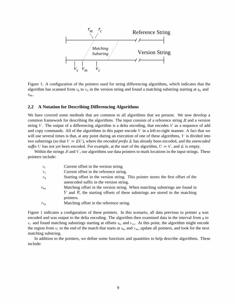
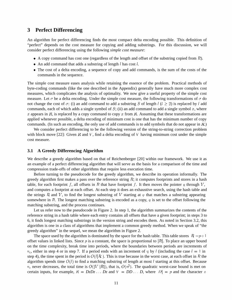
Figure 1: A configuration of the pointers used for string differencing algorithms, which indicates that thealgorithm has scanned from vs to vc in the version string and found a matching substring starting at rm andvm.

2.2 A Notation for Describing Differencing Algorithms

We have covered some methods that are common to all algorithms that we present. We now develop acommon framework for describing the algorithms. The input consists of a reference string R and a versionstring V . The output of a differencing algorithm is a delta encoding, that encodes V as a sequence of addand copy commands. All of the algorithms in this paper encode V in a left-to-right manner. A fact that wewill use several times is that, at any point during an execution of one of these algorithms, V is divided intotwo substrings (so that V = EU ), where the encoded prefix E has already been encoded, and the unencodedsuffix U has not yet been encoded. For example, at the start of the algorithm, U = V , and E is empty.

Within the strings R and V , our algorithms use data pointers to mark locations in the input strings. Thesepointers include:

vc Current offset in the version string.rc Current offset in the reference string.vs Starting offset in the version string. This pointer stores the first offset of the

unencoded suffix in the version string.vm Matching offset in the version string. When matching substrings are found in

V and R, the starting offsets of these substrings are stored in the matchingpointers.

rm Matching offset in the reference string.

Figure 1 indicates a configuration of these pointers. In this scenario, all data previous to pointer vs wasencoded and was output to the delta encoding. The algorithm then examined data in the interval from vs tovc and found matching substrings starting at offsets vm and rm. At this point, the algorithm might encodethe region from vs to the end of the match that starts at vm and rm, update all pointers, and look for the nextmatching substring.

In addition to the pointers, we define some functions and quantities to help describe algorithms. Theseinclude:

9

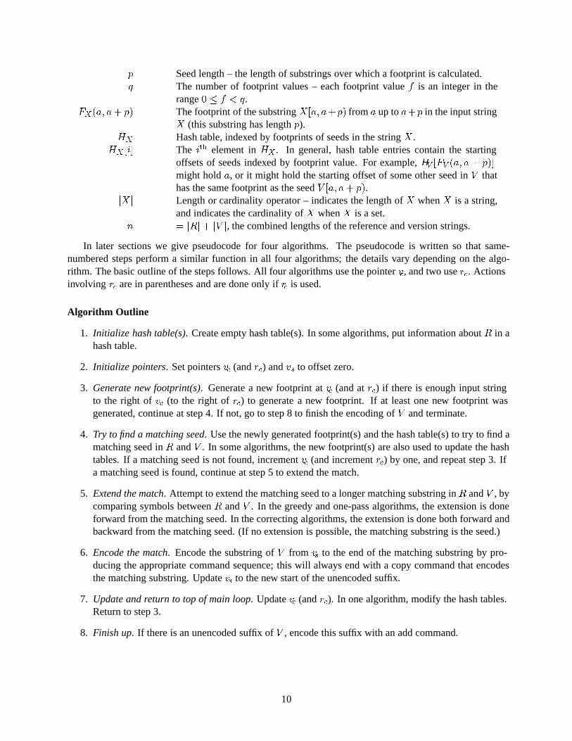
p Seed length – the length of substrings over which a footprint is calculated.q The number of footprint values – each footprint value f is an integer in the

range 0 � f < q.FX(a; a+ p) The footprint of the substring X[a; a+p) from a up to a+p in the input string

X (this substring has length p).HX Hash table, indexed by footprints of seeds in the string X .

HX [i] The ith element in HX . In general, hash table entries contain the startingoffsets of seeds indexed by footprint value. For example, HV [FV (a; a + p)]might hold a, or it might hold the starting offset of some other seed in V thathas the same footprint as the seed V [a; a+ p).

jXj Length or cardinality operator – indicates the length of X when X is a string,and indicates the cardinality of X when X is a set.

n = jRj+ jV j, the combined lengths of the reference and version strings.

In later sections we give pseudocode for four algorithms. The pseudocode is written so that same-numbered steps perform a similar function in all four algorithms; the details vary depending on the algo-rithm. The basic outline of the steps follows. All four algorithms use the pointer vc, and two use rc. Actionsinvolving rc are in parentheses and are done only if rc is used.

Algorithm Outline

1. Initialize hash table(s). Create empty hash table(s). In some algorithms, put information about R in ahash table.

2. Initialize pointers. Set pointers vc (and rc) and vs to offset zero.

3. Generate new footprint(s). Generate a new footprint at vc (and at rc) if there is enough input stringto the right of vc (to the right of rc) to generate a new footprint. If at least one new footprint wasgenerated, continue at step 4. If not, go to step 8 to finish the encoding of V and terminate.

4. Try to find a matching seed. Use the newly generated footprint(s) and the hash table(s) to try to find amatching seed in R and V . In some algorithms, the new footprint(s) are also used to update the hashtables. If a matching seed is not found, increment vc (and increment rc) by one, and repeat step 3. Ifa matching seed is found, continue at step 5 to extend the match.

5. Extend the match. Attempt to extend the matching seed to a longer matching substring in R and V , bycomparing symbols between R and V . In the greedy and one-pass algorithms, the extension is doneforward from the matching seed. In the correcting algorithms, the extension is done both forward andbackward from the matching seed. (If no extension is possible, the matching substring is the seed.)

6. Encode the match. Encode the substring of V from vs to the end of the matching substring by pro-ducing the appropriate command sequence; this will always end with a copy command that encodesthe matching substring. Update vs to the new start of the unencoded suffix.

7. Update and return to top of main loop. Update vc (and rc). In one algorithm, modify the hash tables.Return to step 3.

8. Finish up. If there is an unencoded suffix of V , encode this suffix with an add command.

10

3 Perfect Differencing

An algorithm for perfect differencing finds the most compact delta encoding possible. This definition of“perfect” depends on the cost measure for copying and adding substrings. For this discussion, we willconsider perfect differencing using the following simple cost measure:

� A copy command has cost one (regardless of the length and offset of the substring copied from R).� An add command that adds a substring of length l has cost l.� The cost of a delta encoding, a sequence of copy and add commands, is the sum of the costs of the

commands in the sequence.

The simple cost measure eases analysis while retaining the essence of the problem. Practical methods ofbyte-coding commands (like the one described in the Appendix) generally have much more complex costmeasures, which complicates the analysis of optimality. We now give a useful property of the simple costmeasure. Let � be a delta encoding. Under the simple cost measure, the following transformations of � donot change the cost of �: (i) an add command to add a substring S of length l (l � 2) is replaced by l addcommands, each of which adds a single symbol of S; (ii) an add command to add a single symbol x, wherex appears in R, is replaced by a copy command to copy x from R. Assuming that these transformations areapplied whenever possible, a delta encoding of minimum cost is one that has the minimum number of copycommands. (In such an encoding, the only use of add commands is to add symbols that do not appear in R.)

We consider perfect differencing to be the following version of the string-to-string correction problemwith block move [22]: Given R and V , find a delta encoding of V having minimum cost under the simplecost measure.

3.1 A Greedy Differencing Algorithm

We describe a greedy algorithm based on that of Reichenberger [20] within our framework. We use it asan example of a perfect differencing algorithm that will serve as the basis for a comparison of the time andcompression trade-offs of other algorithms that require less execution time.

Before turning to the pseudocode for the greedy algorithm, we describe its operation informally. Thegreedy algorithm first makes a pass over the reference string R; it computes footprints and stores in a hashtable, for each footprint f , all offsets in R that have footprint f . It then moves the pointer vc through V ,and computes a footprint at each offset. At each step it does an exhaustive search, using the hash table andthe strings R and V , to find the longest substring of V starting at vc that matches a substring appearingsomewhere in R. The longest matching substring is encoded as a copy, vc is set to the offset following thematching substring, and the process continues.

Let us refer now to the pseudocode in Figure 2. In step 1, the algorithm summarizes the contents of thereference string in a hash table where each entry contains all offsets that have a given footprint; in steps 3 to6, it finds longest matching substrings in the version string and encodes them. As noted in Section 3.2, thisalgorithm is one in a class of algorithms that implement a common greedy method. When we speak of “thegreedy algorithm” in the sequel, we mean the algorithm in Figure 2.

The space used by the algorithm is dominated by the space for the hash table. This table stores jRj�p+1offset values in linked lists. Since p is a constant, the space is proportional to jRj. To place an upper boundon the time complexity, break time into periods, where the boundaries between periods are increments ofvc, either in step 4 or in step 7. If a period ends with an increment of vc by l (including the case l = 1 instep 4), the time spent in the period is O(ljRj). This is true because in the worst case, at each offset in R thealgorithm spends time O(l) to find a matching substring of length at most l starting at this offset. Becausevc never decreases, the total time is O(jV jjRj), that is, O(n2). The quadratic worst-case bound is met oncertain inputs, for example, R = DzDz : : : Dz and V = DD : : : D, where jDj = p and the character z

11

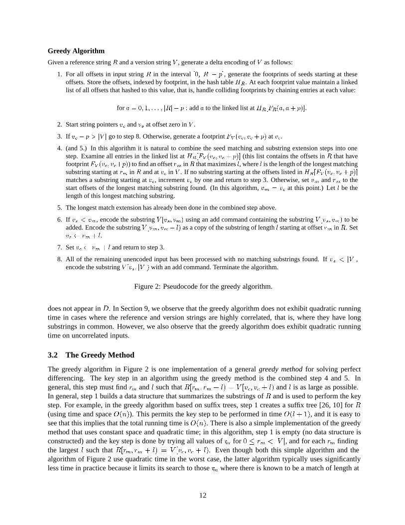
Greedy Algorithm

Given a reference string R and a version string V , generate a delta encoding of V as follows:

1. For all offsets in input string R in the interval [0; jRj � p], generate the footprints of seeds starting at theseoffsets. Store the offsets, indexed by footprint, in the hash table HR. At each footprint value maintain a linkedlist of all offsets that hashed to this value, that is, handle colliding footprints by chaining entries at each value:

for a = 0; 1; : : : ; jRj � p : add a to the linked list at HR[FR(a; a+ p)]:

2. Start string pointers vc and vs at offset zero in V .

3. If vc + p > jV j go to step 8. Otherwise, generate a footprint FV (vc; vc + p) at vc.

4. (and 5.) In this algorithm it is natural to combine the seed matching and substring extension steps into onestep. Examine all entries in the linked list at HR[FV (vc; vc + p)] (this list contains the offsets in R that havefootprintFV (vc; vc+p)) to find an offset rm inR that maximizes l, where l is the length of the longest matchingsubstring starting at rm in R and at vc in V . If no substring starting at the offsets listed in HR[FV (vc; vc + p)]matches a substring starting at vc, increment vc by one and return to step 3. Otherwise, set vm and rm to thestart offsets of the longest matching substring found. (In this algorithm, vm = vc at this point.) Let l be thelength of this longest matching substring.

5. The longest match extension has already been done in the combined step above.

6. If vs < vm, encode the substring V [vs; vm) using an add command containing the substring V [vs; vm) to beadded. Encode the substring V [vm; vm + l) as a copy of the substring of length l starting at offset rm in R. Setvs vm + l.

7. Set vc vm + l and return to step 3.

8. All of the remaining unencoded input has been processed with no matching substrings found. If vs < jV j,encode the substring V [vs; jV j) with an add command. Terminate the algorithm.

Figure 2: Pseudocode for the greedy algorithm.

does not appear in D. In Section 9, we observe that the greedy algorithm does not exhibit quadratic runningtime in cases where the reference and version strings are highly correlated, that is, where they have longsubstrings in common. However, we also observe that the greedy algorithm does exhibit quadratic runningtime on uncorrelated inputs.

3.2 The Greedy Method

The greedy algorithm in Figure 2 is one implementation of a general greedy method for solving perfectdifferencing. The key step in an algorithm using the greedy method is the combined step 4 and 5. Ingeneral, this step must find rm and l such that R[rm; rm + l) = V [vc; vc + l) and l is as large as possible.In general, step 1 builds a data structure that summarizes the substrings of R and is used to perform the keystep. For example, in the greedy algorithm based on suffix trees, step 1 creates a suffix tree [26, 10] for R(using time and space O(n)). This permits the key step to be performed in time O(l + 1), and it is easy tosee that this implies that the total running time is O(n). There is also a simple implementation of the greedymethod that uses constant space and quadratic time; in this algorithm, step 1 is empty (no data structure isconstructed) and the key step is done by trying all values of rm for 0 � rm < jV j, and for each rm findingthe largest l such that R[rm; rm + l) = V [vc; vc + l). Even though both this simple algorithm and thealgorithm of Figure 2 use quadratic time in the worst case, the latter algorithm typically uses significantlyless time in practice because it limits its search to those rm where there is known to be a match of length at

12

least p.

3.3 Proving that the Greedy Algorithm Finds an Optimal Delta Encoding

Tichy [22] has proved that any implementation of the greedy method is a solution to perfect differencing.Here we give a version of Tichy’s proof that appears simpler; in particular, no case analysis is needed.Although we give the proof for the specific greedy algorithm above, the only properties of the algorithmused are that it implements the greedy method.

We show that if p � 2, the greedy algorithm always finds a delta encoding of minimum cost, under thesimple cost measure defined above. If p > 2, the algorithm might not find matching substrings of length2, so it might not find a delta of minimum cost. (The practical advantage of choosing a larger p is that itdecreases the likelihood of finding spurious matches, as described in Section 2.1.3.)

Let R and V be given. Let M be a delta encoding of minimum cost for this R and V , and let G be thedelta encoding found by the greedy algorithm. We let jM j and jGj denote the cost of M and G, respectively.Each symbol of V that does not appear in R must be encoded by an add command in both M and G.Because the greedy algorithm encodes V in a left-to-right manner, it suffices to show, for each maximallength substring S of V containing only symbols that appear in R, that the greedy algorithm finds a delta ofminimum cost when given R and S. As noted above, the simple cost of a delta encoding does not increaseif an add command of length l is replaced by l add commands that copy single symbols. Therefore, for R,V , M , and G as above, it suffices to show that jGj = jM j in the case where every symbol of V appears in Rand where M and G contain only copy commands. Because the cost of a copy command is one, jM j (resp.,jGj) equals the number of copy commands in M (resp., G).

For j � 1, let xj be the largest integer such that V [0; xj) can be encoded by j copy commands. Also,let x0 = 0. Let t be the smallest integer such that xt = jV j. The minimality of t implies that x0 < x1 <� � � < xt. By the definition of t, the cost of M is t. To complete the proof we show by induction on j that,for 0 � j � t, the first j copy commands in G encode V [0; xj). Taking j = t, this implies that the cost ofG is t, so jGj = jM j. The base case j = 0 is obvious, where we view V [0; 0) as the empty string. Fix jwith 0 � j < t, and assume by induction that the first j copy commands in G encode V [0; xj). It followsfrom the definition of the greedy algorithm (more generally, the greedy method) that its (j + 1)th copycommand will encode the longest substring S that starts at offset xj in V and is a substring of R. Becausethe longest prefix of V that can be encoded by j copies is V [0; xj), and j+1 copies can encode V [0; xj+1),it follows that V [xj; xj+1) is a substring Sj of R. Therefore, the greedy algorithm will encode S = Sj withits (j + 1)th copy command, and the first j + 1 copy commands in G encode [0; xj+1). This completes theinductive step, and so completes the proof that jGj = jM j.

4 Differencing in Linear Time and Constant Space

While perfect differencing provides optimally compressed output, the existing methods for perfect differ-encing do not provide acceptable time and space performance. As we are interested in algorithms that scalewell and can difference arbitrarily large inputs, we focus on the task of differencing in linear time and con-stant space. We now present such an algorithm. This algorithm, termed the “one-pass” algorithm, uses basicmethods for substring matching, and will serve as a departure point for examining further algorithms thatuse additional methods to improve compression.

4.1 The One-Pass Differencing Algorithm

The one-pass differencing algorithm finds a delta encoding in linear time and constant space. It finds match-ing substrings in a “next match” sense. That is, after copy-encoding a matching substring, the algorithm

13

looks for the next matching substring forward in both input strings. It does this by flushing the hash tablesafter encoding a copy. The effect is that, in the future, the one-pass algorithm ignores the portion of R and Vthat precedes the end of the substring that was just copy-encoded. The next match policy detects matchingsubstrings sequentially. As a consequence, in the presence of transposed data (with R as : : :X : : : Y : : : andV as : : : Y : : :X : : : ), the algorithm will not detect both of the matching substrings X and Y .

The algorithm scans forward in both input strings and summarizes the seeds that it has seen by foot-printing them and storing their offsets in two hash tables, one for R and one for V . The algorithm usesthe footprints in the hash tables to detect matching seeds, and it then extends the match forward as far aspossible. Unlike the greedy algorithm, the one-pass algorithm does not store all offsets having a certainfootprint; instead it stores, for each footprint, at most one offset in R and at most one in V . This makes thehash table for R smaller (size q rather than jRj) and more easily searched, but the compression is not alwaysoptimal. At the start of the algorithm, and after each flush of the hash tables, the stored offset in R (resp.,V ) is the first one found in R (resp., V ) having the given footprint. Pseudocode for the one-pass algorithmis in Figure 3.

Retaining the first-found offset for each seed is the correct way to implement the next match policy inthe following sense, assuming that the hash function is ideal. We say that a hash function F is ideal for Rand V when, for all seeds s1 and s2 that appear in either R or V , if s1 6= s2 then F (s1) 6= F (s2). Consideran arbitrary time when step 3 is entered, either for the first time or just after the hash tables have been flushedin step 7. At this point the hash tables are empty and the algorithm is starting “fresh” to find another match(rm; vm) with rc � rm and vc � vm. We say that a pair (r; v) of offsets is a match if the seeds at offsets rand v are identical. It is not hard to see that if the match (rm; vm) is found at this iteration of steps 3–7, thenthere does not exist a match (r0m; v

0m) 6= (rm; vm) with rc � r0m � rm and vc � v0m � vm. This property

can be violated if the hash function is not ideal, as discussed in Section 4.3.The one-pass differencing algorithm focuses on finding pairs of synchronized offsets in R and V , which

indicates that the data at the synchronized offset in R is the same as the data at the synchronized offset inV . The algorithm switches between hashing mode (steps 3 and 4) where it attempts to find synchronizedoffsets, and identity mode (step 5) where it extends the match forward as far as possible. When a matchis found and the algorithm enters identity mode, the pointers are “synchronized”. When the identity testfails at step 5, the strings differ and the string offsets are again “out of synch”. The algorithm then restartshashing to regain the location of common data in the two strings.

In Section 10, we show that differencing algorithms that take a single pass over the input strings, with norandom access allowed, achieve sub-optimal compression when data are transposed (i.e., when substringsoccur in a different order in the reference and version strings). The one-pass algorithm is not a strict singlepass algorithm in the sense of Section 10, as it performs random access in both strings to verify the identity ofsubstrings with matching footprints. However, it does exhibit the limitations of a strict single pass algorithmin the presence of transpositions, because after finding a match it limits its search space for subsequentmatches to only the offsets greater than the end of the previous matching substring.

4.2 Time and Space Analysis

We now show that the one-pass algorithm uses time linear in np + q and space linear in q; recall that q isthe number of footprint values (that is, the number of entries in each hash table), and n = jRj + jV j.2 Wealways use the algorithm with p a (small) constant and q a (large) constant (i.e., p and q do not depend onn). In this case, the running time is O(n) and the space is O(1) in the worst case.

2The term np is needed to handle the worst-case situation that step 4b is executed approximately n times, and at each executionof this step the algorithm spends time p to discover that seeds with the same footprint are not identical. In practice, we would notexpect this worst-case situation to happen.

14

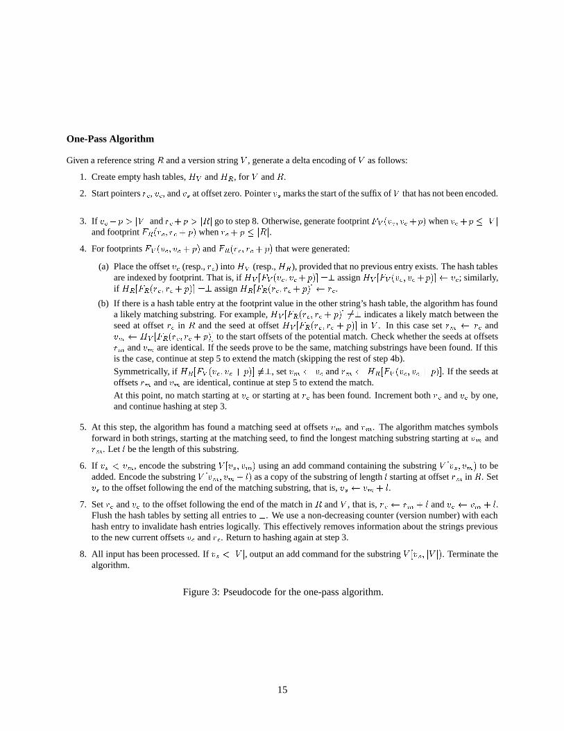
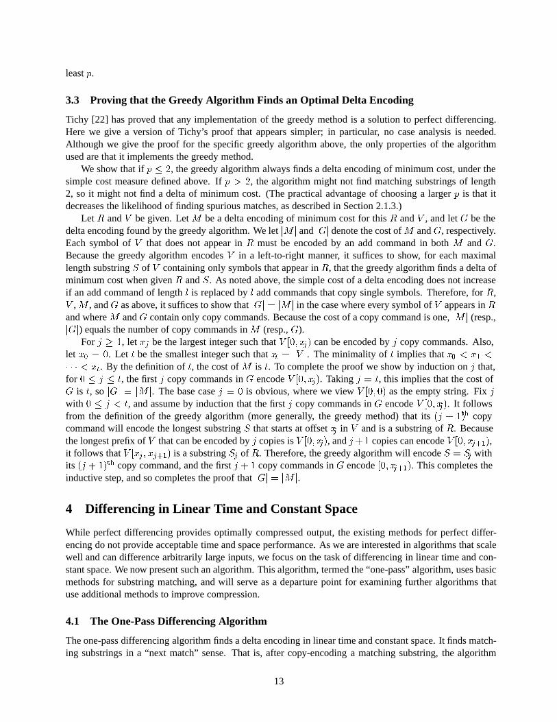
One-Pass Algorithm

Given a reference string R and a version string V , generate a delta encoding of V as follows:

1. Create empty hash tables, HV and HR, for V and R.

2. Start pointers rc, vc, and vs at offset zero. Pointer vs marks the start of the suffix of V that has not been encoded.

3. If vc+ p > jV j and rc+ p > jRj go to step 8. Otherwise, generate footprint FV (vc; vc+ p) when vc+ p � jV jand footprint FR(rc; rc + p) when rc + p � jRj.

4. For footprints FV (vc; vc + p) and FR(rc; rc + p) that were generated:

(a) Place the offset vc (resp., rc) into HV (resp., HR), provided that no previous entry exists. The hash tablesare indexed by footprint. That is, if HV [FV (vc; vc+ p)] =? assign HV [FV (vc; vc+ p)] vc; similarly,if HR[FR(rc; rc + p)] =? assign HR[FR(rc; rc + p)] rc.

(b) If there is a hash table entry at the footprint value in the other string’s hash table, the algorithm has founda likely matching substring. For example, HV [FR(rc; rc + p)] 6=? indicates a likely match between theseed at offset rc in R and the seed at offset HV [FR(rc; rc + p)] in V . In this case set rm rc andvm HV [FR(rc; rc + p)] to the start offsets of the potential match. Check whether the seeds at offsetsrm and vm are identical. If the seeds prove to be the same, matching substrings have been found. If thisis the case, continue at step 5 to extend the match (skipping the rest of step 4b).Symmetrically, if HR[FV (vc; vc + p)] 6=?, set vm vc and rm HR[FV (vc; vc + p)]. If the seeds atoffsets rm and vm are identical, continue at step 5 to extend the match.At this point, no match starting at vc or starting at rc has been found. Increment both rc and vc by one,and continue hashing at step 3.

5. At this step, the algorithm has found a matching seed at offsets vm and rm. The algorithm matches symbolsforward in both strings, starting at the matching seed, to find the longest matching substring starting at vm andrm. Let l be the length of this substring.

6. If vs < vm, encode the substring V [vs; vm) using an add command containing the substring V [vs; vm) to beadded. Encode the substring V [vm; vm + l) as a copy of the substring of length l starting at offset rm in R. Setvs to the offset following the end of the matching substring, that is, vs vm + l.

7. Set rc and vc to the offset following the end of the match in R and V , that is, rc rm + l and vc vm + l.Flush the hash tables by setting all entries to ?. We use a non-decreasing counter (version number) with eachhash entry to invalidate hash entries logically. This effectively removes information about the strings previousto the new current offsets vc and rc. Return to hashing again at step 3.

8. All input has been processed. If vs < jV j, output an add command for the substring V [vs; jV j). Terminate thealgorithm.

Figure 3: Pseudocode for the one-pass algorithm.

15

Theorem 4.1 If the one-pass algorithm is run with seed length p, the number of footprints equal to q, andinput strings of total length n, then the algorithm runs in time O(np+ q) and space O(q).

Proof. The constants implicit in all occurrences of the O-notation do not depend on p, q, R, V , or n.The space bound is clear. At all times, the algorithm maintains two hash tables, each of which contains

q entries. After finding a match, hash entries are flushed and the same hash tables are reused to find the nextmatching substring. Except for the hash tables, the algorithm uses space O(1). So the total space is O(q).

We now show the time bound. Initially, during steps 1 and 2, the algorithm takes time O(q). Forthe remainder of the run of the algorithm, divide time into periods, where the boundaries between periodsare the times when the algorithm enters hashing mode; this occurs for the first time when it moves fromstep 2 to step 3, and subsequently every time it moves from step 7 to step 3. Focus on an arbitrary period,and let r0c and v0c be the values of rc and vc at the start of the period. In particular, the start vs of theunencoded suffix is v0c . At this point, the hash tables are empty. We follow the run of the algorithm duringthis period, and bound the time used during the period in terms of the net amount that the pointers rc andvc advance during the period. (By “net”, we mean that we subtract from the net advancement when apointer moves backwards.) When rc and vc are advancing in hashing mode (repetitions of steps 3 and 4),the algorithm uses time O(p) each time that these pointers advance by one. When a matching seed is foundin step 4b, either (i) v0c � vm = vc and r0c � rm � rc, or (ii) r0c � rm = rc and v0c � vm � vc. LetM = max(vm� v0c ; rm� r0c ). (The following also covers the case that the algorithm moves to the finishingstep 8 before a match is found.) Because either vm = vc or rm = rc, the total time spent in hashing mode isO(pM). The number of non-? hash table entries at this point is at most 2M . The match extension step 5takes time O(l). The encoding step 6 takes time O(vm � v0c ), that is, O(M). In step 7, the pointers vc andrc are reset to the end of the match; let v1c = vm + l and r1c = rm + l be the values of vc and rc after this isdone. These are also the values of these pointers at the start of the next period. It follows that:

1. vc and rc advanced by a total net amount of at least M + 2l during the period(i.e., (v1c � v0c ) + (r1c � r0c ) �M + 2l), and

2. the time spent in the period was O(pM + l).

It follows that the algorithm runs in time O(np+ q), as we now show. Let t be the number of periods, andfor 1 � i � t let Mi and li be the values of M and l, respectively, for period i. Let M� (resp., l�) be thesum of Mi (resp., li) over 1 � i � t. Because the pointers can advance by a total net amount of at mostn = jRj+ jV j during the entire run, statement 1 above implies that M� + 2l� � n. Initially, during steps 1and 2, the algorithm takes time O(q). By statement 2 above, the algorithm uses time O(pM� + l�) duringall t periods. It follows that the total time is O(np+ q). �

4.3 Sub-Optimal Compression

In addition to failing to detect transposed data, the one-pass algorithm achieves less than optimal compres-sion when it falsely believes that the offsets are synchronized or when the hash function exhibits less thanideal behavior. (Recall that a hash function is “ideal” if it is one-to-one on the set of seeds that appear in Rand V .) We now consider each of these issues.

When we say that the algorithm falsely believes that the offsets are synchronized, we are referring to“spurious” or “coincidental” matches (as discussed in x2.1.3), which arise as a result of taking the next matchrather than the best match. These collisions occur when the algorithm believes that it has found synchronizedoffsets between the strings when in actuality the collision just happens to be between substrings whoselength-p prefixes match by chance, and a longer matching substring exists at another offset. An example ofa spurious match is shown in Figure 4. Call the substring ABCDEFG the “long match” in R and V . In this

16

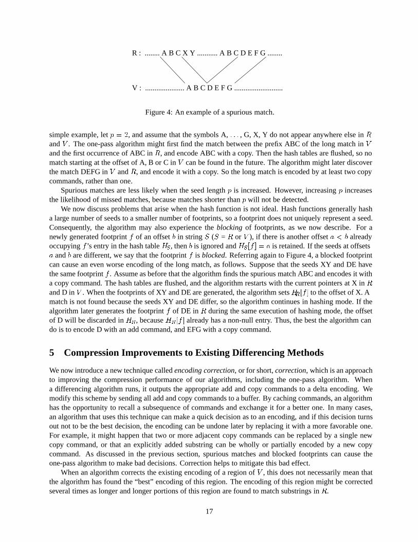
R : ........ A B C X Y ........... A B C D E F G ........

V : ..................... A B C D E F G ..........................

Figure 4: An example of a spurious match.

simple example, let p = 2, and assume that the symbols A, : : : , G, X, Y do not appear anywhere else in Rand V . The one-pass algorithm might first find the match between the prefix ABC of the long match in Vand the first occurrence of ABC in R, and encode ABC with a copy. Then the hash tables are flushed, so nomatch starting at the offset of A, B or C in V can be found in the future. The algorithm might later discoverthe match DEFG in V and R, and encode it with a copy. So the long match is encoded by at least two copycommands, rather than one.

Spurious matches are less likely when the seed length p is increased. However, increasing p increasesthe likelihood of missed matches, because matches shorter than p will not be detected.

We now discuss problems that arise when the hash function is not ideal. Hash functions generally hasha large number of seeds to a smaller number of footprints, so a footprint does not uniquely represent a seed.Consequently, the algorithm may also experience the blocking of footprints, as we now describe. For anewly generated footprint f of an offset b in string S (S = R or V ), if there is another offset a < b alreadyoccupying f ’s entry in the hash table HS , then b is ignored and HS [f ] = a is retained. If the seeds at offsetsa and b are different, we say that the footprint f is blocked. Referring again to Figure 4, a blocked footprintcan cause an even worse encoding of the long match, as follows. Suppose that the seeds XY and DE havethe same footprint f . Assume as before that the algorithm finds the spurious match ABC and encodes it witha copy command. The hash tables are flushed, and the algorithm restarts with the current pointers at X in Rand D in V . When the footprints of XY and DE are generated, the algorithm sets HR[f ] to the offset of X. Amatch is not found because the seeds XY and DE differ, so the algorithm continues in hashing mode. If thealgorithm later generates the footprint f of DE in R during the same execution of hashing mode, the offsetof D will be discarded in HR, because HR[f ] already has a non-null entry. Thus, the best the algorithm cando is to encode D with an add command, and EFG with a copy command.

5 Compression Improvements to Existing Differencing Methods

We now introduce a new technique called encoding correction, or for short, correction, which is an approachto improving the compression performance of our algorithms, including the one-pass algorithm. Whena differencing algorithm runs, it outputs the appropriate add and copy commands to a delta encoding. Wemodify this scheme by sending all add and copy commands to a buffer. By caching commands, an algorithmhas the opportunity to recall a subsequence of commands and exchange it for a better one. In many cases,an algorithm that uses this technique can make a quick decision as to an encoding, and if this decision turnsout not to be the best decision, the encoding can be undone later by replacing it with a more favorable one.For example, it might happen that two or more adjacent copy commands can be replaced by a single newcopy command, or that an explicitly added substring can be wholly or partially encoded by a new copycommand. As discussed in the previous section, spurious matches and blocked footprints can cause theone-pass algorithm to make bad decisions. Correction helps to mitigate this bad effect.

When an algorithm corrects the existing encoding of a region of V , this does not necessarily mean thatthe algorithm has found the “best” encoding of this region. The encoding of this region might be correctedseveral times as longer and longer portions of this region are found to match substrings in R.

17

To implement correction, the algorithm inserts add and copy commands into a buffer rather than writingthem directly to the delta encoding. The buffer, in this instance, is a FIFO queue of commands called theencoding lookback buffer, or for short, the buffer. When a substring of the version string is encoded, theappropriate command is written to the buffer. The buffer collects commands until it is full. Then, whenwriting a command to a full buffer, the oldest command gets pushed out and is written to the delta encoding.When a command “falls out of the buffer” it becomes immutable and has been committed to the deltaencoding. In theory, the buffer can have unlimited size, so that commands never fall out. But in practice, itis useful for the buffer to be implemented in memory so that operations on the buffer can be done efficiently,and this limits the size of the buffer.

The objects in the buffer are not strictly add and copy commands, as defined in Section 2.1.1. In partic-ular, an add command in the buffer does not contain the added substring. However, each command in thebuffer is associated with its version offset, the starting offset of the substring in the version string that thiscommand encodes. The length and version offset stored with an add command permit the added substringto be found in V when the add command exits the buffer. In addition, the version offsets in the buffer areincreasing and distinct. This permits the use of binary search to find commands in the buffer by their versionoffsets. For simplicity, we refer to the objects in the buffer as “commands”, because each object in the bufferspecifies a unique add or copy command.

Correction can cause algorithmic running time to depart from a strict linear worst-case bound. But onall experimental inputs (as discussed in Section 9) the one-pass algorithm with correction displays timeperformance similar to that of the original one-pass algorithm, and the compression is much improved.

5.1 Editing the Encoding Lookback Buffer

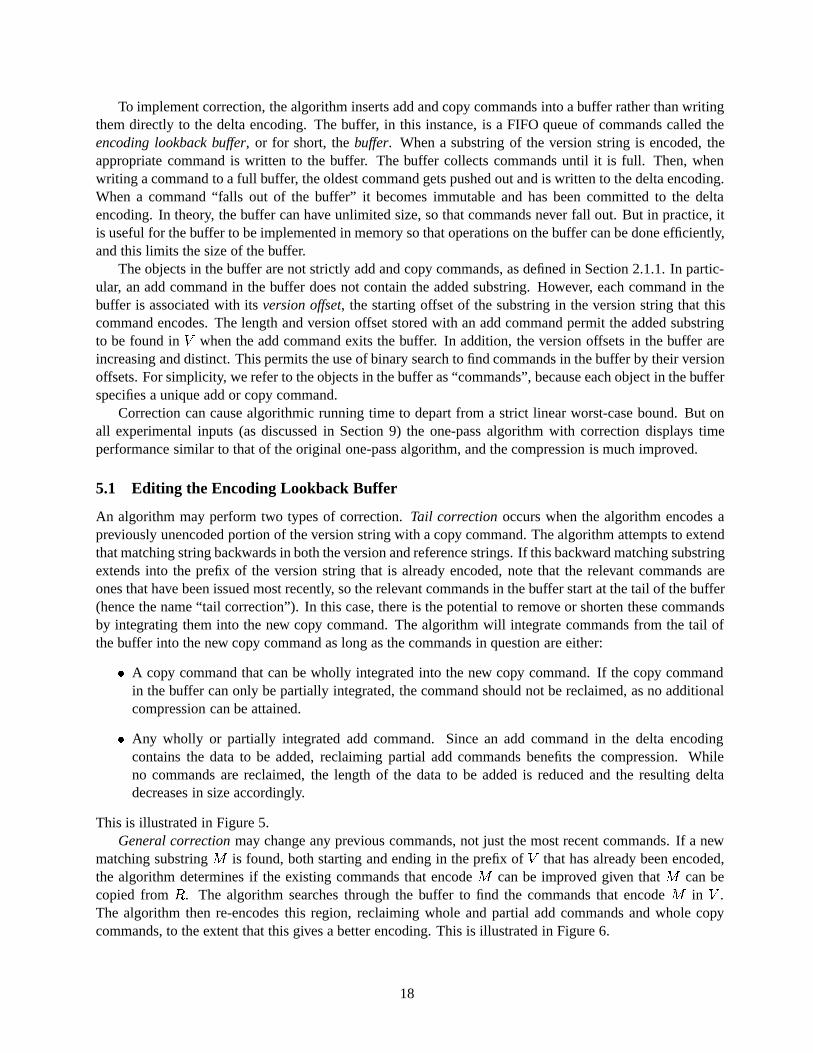
An algorithm may perform two types of correction. Tail correction occurs when the algorithm encodes apreviously unencoded portion of the version string with a copy command. The algorithm attempts to extendthat matching string backwards in both the version and reference strings. If this backward matching substringextends into the prefix of the version string that is already encoded, note that the relevant commands areones that have been issued most recently, so the relevant commands in the buffer start at the tail of the buffer(hence the name “tail correction”). In this case, there is the potential to remove or shorten these commandsby integrating them into the new copy command. The algorithm will integrate commands from the tail ofthe buffer into the new copy command as long as the commands in question are either:

� A copy command that can be wholly integrated into the new copy command. If the copy commandin the buffer can only be partially integrated, the command should not be reclaimed, as no additionalcompression can be attained.

� Any wholly or partially integrated add command. Since an add command in the delta encodingcontains the data to be added, reclaiming partial add commands benefits the compression. Whileno commands are reclaimed, the length of the data to be added is reduced and the resulting deltadecreases in size accordingly.

This is illustrated in Figure 5.General correction may change any previous commands, not just the most recent commands. If a new

matching substring M is found, both starting and ending in the prefix of V that has already been encoded,the algorithm determines if the existing commands that encode M can be improved given that M can becopied from R. The algorithm searches through the buffer to find the commands that encode M in V .The algorithm then re-encodes this region, reclaiming whole and partial add commands and whole copycommands, to the extent that this gives a better encoding. This is illustrated in Figure 6.

18

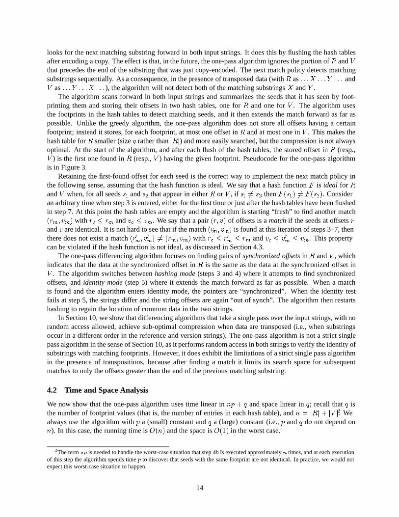
unencoded

Buffer After

unencoded

matching substring

add copy add copy

add copy

copyadd add copy

add copy

tail

tail

. . .

. . .

. . .

. . .

. . .

. . . Buffer Before

V Before

V After

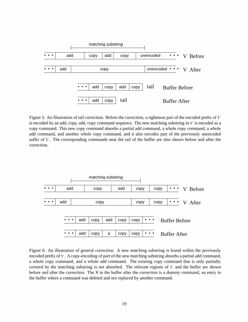
Figure 5: An illustration of tail correction. Before the correction, a rightmost part of the encoded prefix of Vis encoded by an add, copy, add, copy command sequence. The new matching substring in V is encoded as acopy command. This new copy command absorbs a partial add command, a whole copy command, a wholeadd command, and another whole copy command, and it also encodes part of the previously unencodedsuffix of V . The corresponding commands near the tail of the buffer are also shown before and after thecorrection.

Buffer After

matching substring

add

add

copy

. . .

. . .

. . .

. . .

V Before

V After

copycopycopy

copy copyadd

add

add. . .

. . .

. . .

. . .

copy copy copy

copycopycopy

add

Buffer Before

X

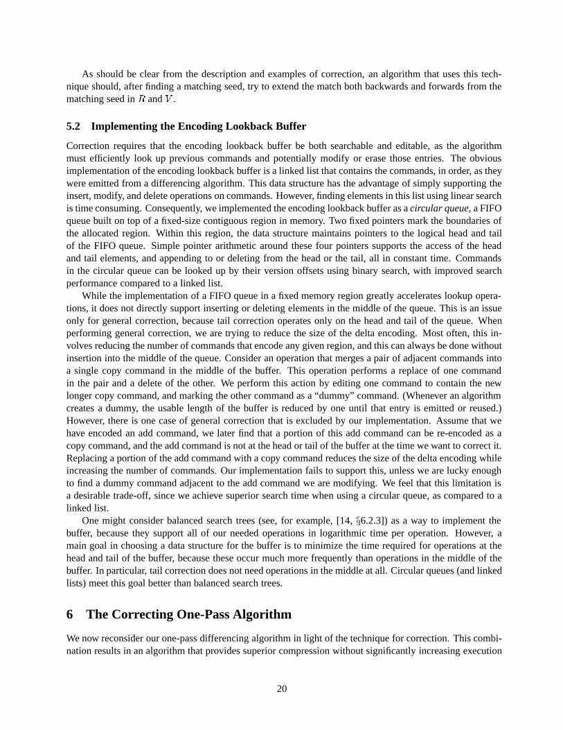
Figure 6: An illustration of general correction. A new matching substring is found within the previouslyencoded prefix of V . A copy-encoding of part of the new matching substring absorbs a partial add command,a whole copy command, and a whole add command. The existing copy command that is only partiallycovered by the matching substring is not absorbed. The relevant regions of V and the buffer are shownbefore and after the correction. The X in the buffer after the correction is a dummy command, an entry inthe buffer where a command was deleted and not replaced by another command.

19

As should be clear from the description and examples of correction, an algorithm that uses this tech-nique should, after finding a matching seed, try to extend the match both backwards and forwards from thematching seed in R and V .

5.2 Implementing the Encoding Lookback Buffer

Correction requires that the encoding lookback buffer be both searchable and editable, as the algorithmmust efficiently look up previous commands and potentially modify or erase those entries. The obviousimplementation of the encoding lookback buffer is a linked list that contains the commands, in order, as theywere emitted from a differencing algorithm. This data structure has the advantage of simply supporting theinsert, modify, and delete operations on commands. However, finding elements in this list using linear searchis time consuming. Consequently, we implemented the encoding lookback buffer as a circular queue, a FIFOqueue built on top of a fixed-size contiguous region in memory. Two fixed pointers mark the boundaries ofthe allocated region. Within this region, the data structure maintains pointers to the logical head and tailof the FIFO queue. Simple pointer arithmetic around these four pointers supports the access of the headand tail elements, and appending to or deleting from the head or the tail, all in constant time. Commandsin the circular queue can be looked up by their version offsets using binary search, with improved searchperformance compared to a linked list.

While the implementation of a FIFO queue in a fixed memory region greatly accelerates lookup opera-tions, it does not directly support inserting or deleting elements in the middle of the queue. This is an issueonly for general correction, because tail correction operates only on the head and tail of the queue. Whenperforming general correction, we are trying to reduce the size of the delta encoding. Most often, this in-volves reducing the number of commands that encode any given region, and this can always be done withoutinsertion into the middle of the queue. Consider an operation that merges a pair of adjacent commands intoa single copy command in the middle of the buffer. This operation performs a replace of one commandin the pair and a delete of the other. We perform this action by editing one command to contain the newlonger copy command, and marking the other command as a “dummy” command. (Whenever an algorithmcreates a dummy, the usable length of the buffer is reduced by one until that entry is emitted or reused.)However, there is one case of general correction that is excluded by our implementation. Assume that wehave encoded an add command, we later find that a portion of this add command can be re-encoded as acopy command, and the add command is not at the head or tail of the buffer at the time we want to correct it.Replacing a portion of the add command with a copy command reduces the size of the delta encoding whileincreasing the number of commands. Our implementation fails to support this, unless we are lucky enoughto find a dummy command adjacent to the add command we are modifying. We feel that this limitation isa desirable trade-off, since we achieve superior search time when using a circular queue, as compared to alinked list.

One might consider balanced search trees (see, for example, [14, x6.2.3]) as a way to implement thebuffer, because they support all of our needed operations in logarithmic time per operation. However, amain goal in choosing a data structure for the buffer is to minimize the time required for operations at thehead and tail of the buffer, because these occur much more frequently than operations in the middle of thebuffer. In particular, tail correction does not need operations in the middle at all. Circular queues (and linkedlists) meet this goal better than balanced search trees.

6 The Correcting One-Pass Algorithm

We now reconsider our one-pass differencing algorithm in light of the technique for correction. This combi-nation results in an algorithm that provides superior compression without significantly increasing execution

20

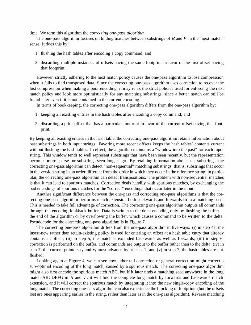
time. We term this algorithm the correcting one-pass algorithm.The one-pass algorithm focuses on finding matches between substrings of R and V in the “next match”

sense. It does this by:

1. flushing the hash tables after encoding a copy command; and

2. discarding multiple instances of offsets having the same footprint in favor of the first offset havingthat footprint.

However, strictly adhering to the next match policy causes the one-pass algorithm to lose compressionwhen it fails to find transposed data. Since the correcting one-pass algorithm uses correction to recover thelost compression when making a poor encoding, it may relax the strict policies used for enforcing the nextmatch policy and look more optimistically for any matching substrings, since a better match can still befound later even if it is not contained in the current encoding.

In terms of bookkeeping, the correcting one-pass algorithm differs from the one-pass algorithm by:

1. keeping all existing entries in the hash tables after encoding a copy command; and

2. discarding a prior offset that has a particular footprint in favor of the current offset having that foot-print.

By keeping all existing entries in the hash table, the correcting one-pass algorithm retains information aboutpast substrings in both input strings. Favoring more recent offsets keeps the hash tables’ contents currentwithout flushing the hash tables. In effect, the algorithm maintains a “window into the past” for each inputstring. This window tends to well represent substrings that have been seen recently, but the representationbecomes more sparse for substrings seen longer ago. By retaining information about past substrings, thecorrecting one-pass algorithm can detect “non-sequential” matching substrings, that is, substrings that occurin the version string in an order different from the order in which they occur in the reference string; in partic-ular, the correcting one-pass algorithm can detect transpositions. The problem with non-sequential matchesis that it can lead to spurious matches. Correction deals handily with spurious matches, by exchanging thebad encodings of spurious matches for the “correct” encodings that occur later in the input.

Another significant difference between the one-pass and correcting one-pass algorithms is that the cor-recting one-pass algorithm performs match extension both backwards and forwards from a matching seed.This is needed to take full advantage of correction. The correcting one-pass algorithm outputs all commandsthrough the encoding lookback buffer. Data is written to the delta encoding only by flushing the buffer atthe end of the algorithm or by overflowing the buffer, which causes a command to be written to the delta.Pseudocode for the correcting one-pass algorithm is in Figure 7.

The correcting one-pass algorithm differs from the one-pass algorithm in five ways: (i) in step 4a, theinsert-new rather than retain-existing policy is used for entering an offset at a hash table entry that alreadycontains an offset; (ii) in step 5, the match is extended backwards as well as forwards; (iii) in step 6,correction is performed on the buffer, and commands are output to the buffer rather than to the delta; (iv) instep 7, the current pointers vc and rc must advance by at least 1; and (v) in step 7, the hash tables are notflushed.

Looking again at Figure 4, we can see how either tail correction or general correction might correct asub-optimal encoding of the long match, caused by a spurious match. The correcting one-pass algorithmmight also first encode the spurious match ABC, but if it later finds a matching seed anywhere in the longmatch ABCDEFG in R and V , it will find the complete long match by forwards and backwards matchextension, and it will correct the spurious match by integrating it into the new single-copy encoding of thelong match. The correcting one-pass algorithm can also experience the blocking of footprints (but the offsetslost are ones appearing earlier in the string, rather than later as in the one-pass algorithm). Reverse matching

21

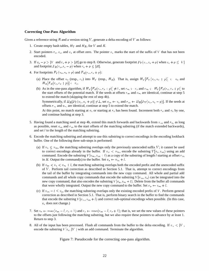
Correcting One-Pass Algorithm

Given a reference string R and a version string V , generate a delta encoding of V as follows:

1. Create empty hash tables, HV and HR, for V and R.

2. Start pointers rc, vc, and vs at offset zero. The pointer vs marks the start of the suffix of V that has not beenencoded.

3. If vc+ p > jV j and rc+ p > jRj go to step 8. Otherwise, generate footprint FV (vc; vc+ p) when vc+ p � jV jand footprint FR(rc; rc + p) when rc + p � jRj.

4. For footprints FV (vc; vc + p) and FR(rc; rc + p):

(a) Place the offset vc (resp., rc) into HV (resp., HR). That is, assign HV [FV (vc; vc + p)] vc andHR[FR(rc; rc + p)] rc.

(b) As in the one-pass algorithm, if HV [FR(rc; rc+ p)] 6=?, set rm rc and vm HV [FR(rc; rc+ p)] tothe start offsets of the potential match. If the seeds at offsets rm and vm are identical, continue at step 5to extend the match (skipping the rest of step 4b).Symmetrically, if HR[FV (vc; vc + p)] 6=?, set vm vc and rm HR[FV (vc; vc + p)]. If the seeds atoffsets rm and vm are identical, continue at step 5 to extend the match.At this point, no match starting at vc or starting at rc has been found. Increment both rc and vc by one,and continue hashing at step 3.

5. Having found a matching seed at step 4b, extend this match forwards and backwards from vm and rm as longas possible, reset vm and rm to the start offsets of the matching substring (if the match extended backwards),and set l to the length of the matching substring.

6. Encode the matching substring and attempt to use this substring to correct encodings in the encoding lookbackbuffer. One of the following three sub-steps is performed:

(a) If vs � vm, the matching substring overlaps only the previously unencoded suffix V ; it cannot be usedto correct encodings already in the buffer. If vs < vm, encode the substring V [vs; vm) using an addcommand. Encode the substring V [vm; vm+ l) as a copy of the substring of length l starting at offset rmin R. Output the command(s) to the buffer. Set vs vm + l.

(b) If vm < vs < vm + l, the matching substring overlaps both the encoded prefix and the unencoded suffixof V . Perform tail correction as described in Section 5.1. That is, attempt to correct encodings fromthe tail of the buffer by integrating commands into the new copy command. All whole and partial addcommands and all whole copy commands that encode the substring V [vm; vs) can be integrated into thenew copy command, that also encodes the substring V [vs; vm + l). Delete from the buffer all commandsthat were wholly integrated. Output the new copy command to the buffer. Set vs vm + l.

(c) If vm + l � vs, the matching substring overlaps only the existing encoded prefix of V . Perform generalcorrection as described in Section 5.1. That is, perform binary search in the buffer to find the commandsthat encode the substring V [vm; vm + l) and correct sub-optimal encodings when possible. (In this case,vs does not change.)

7. Set vc max(vm + l; vc + 1) and rc max(rm + l; rc + 1); that is, we set the new values of these pointersto the offsets just following the matching substring, but we also require these pointers to advance by at least 1.Return to step 3.

8. All of the input has been processed. Flush all commands from the buffer to the delta encoding. If vs < jV j,encode the substring V [vs; jV j) with an add command. Terminate the algorithm.

Figure 7: Pseudocode for the correcting one-pass algorithm.

22

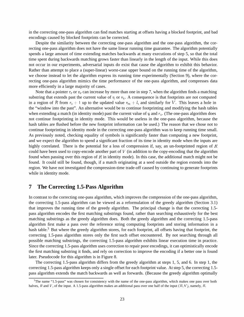
in the correcting one-pass algorithm can find matches starting at offsets having a blocked footprint, and badencodings caused by blocked footprints can be corrected.

Despite the similarity between the correcting one-pass algorithm and the one-pass algorithm, the cor-recting one-pass algorithm does not have the same linear running time guarantee. The algorithm potentiallyspends a large amount of time extending matches backwards at many executions of step 5, so that the totaltime spent during backwards matching grows faster than linearly in the length of the input. While this doesnot occur in our experiments, adversarial inputs do exist that cause the algorithm to exhibit this behavior.Rather than attempt to place a (super-linear) worst-case upper bound on the running time of the algorithm,we choose instead to let the algorithm express its running time experimentally (Section 9), where the cor-recting one-pass algorithm mimics the time performance of the one-pass algorithm, and compresses datamore efficiently in a large majority of cases.

Note that a pointer rc or vc can increase by more than one in step 7, when the algorithm finds a matchingsubstring that extends past the current value of rc or vc. A consequence is that footprints are not computedin a region of R from rc + 1 up to the updated value rm + l, and similarly for V . This leaves a hole inthe “window into the past”. An alternative would be to continue footprinting and modifying the hash tableswhen extending a match (in identity mode) past the current value of vc and rc. (The one-pass algorithm doesnot continue footprinting in identity mode. This would be useless in the one-pass algorithm, because thehash tables are flushed before the new footprint information can be used.) The reason that we chose not tocontinue footprinting in identity mode in the correcting one-pass algorithm was to keep running time small.As previously noted, checking equality of symbols is significantly faster than computing a new footprint,and we expect the algorithm to spend a significant fraction of its time in identity mode when the inputs arehighly correlated. There is the potential for a loss of compression if, say, an un-footprinted region of Rcould have been used to copy-encode another part of V (in addition to the copy-encoding that the algorithmfound when passing over this region of R in identity mode). In this case, the additional match might not befound. It could still be found, though, if a match originating at a seed outside the region extends into theregion. We have not investigated the compression-time trade-off caused by continuing to generate footprintswhile in identity mode.

7 The Correcting 1.5-Pass Algorithm

In contrast to the correcting one-pass algorithm, which improves the compression of the one-pass algorithm,the correcting 1.5-pass algorithm can be viewed as a reformulation of the greedy algorithm (Section 3.1)that improves the running time of the greedy algorithm. The principal change is that the correcting 1.5-pass algorithm encodes the first matching substrings found, rather than searching exhaustively for the bestmatching substrings as the greedy algorithm does. Both the greedy algorithm and the correcting 1.5-passalgorithm first make a pass over the reference string computing footprints and storing information in ahash table.3 But where the greedy algorithm stores, for each footprint, all offsets having that footprint, thecorrecting 1.5-pass algorithm stores only the first such offset encountered. By not searching through allpossible matching substrings, the correcting 1.5-pass algorithm exhibits linear execution time in practice.Since the correcting 1.5-pass algorithm uses correction to repair poor encodings, it can optimistically encodethe first matching substring it finds, and rely on correction to improve the encoding if a better one is foundlater. Pseudocode for this algorithm is in Figure 8.

The correcting 1.5-pass algorithm differs from the greedy algorithm at steps 1, 5, and 6. In step 1, thecorrecting 1.5-pass algorithm keeps only a single offset for each footprint value. At step 5, the correcting 1.5-pass algorithm extends the match backwards as well as forwards. (Because the greedy algorithm optimally

3The name “1.5-pass” was chosen for consistency with the name of the one-pass algorithm, which makes one pass over bothhalves, R and V , of the input. A 1.5-pass algorithm makes an additional pass over one half of the input (R;V ), namely, R.

23

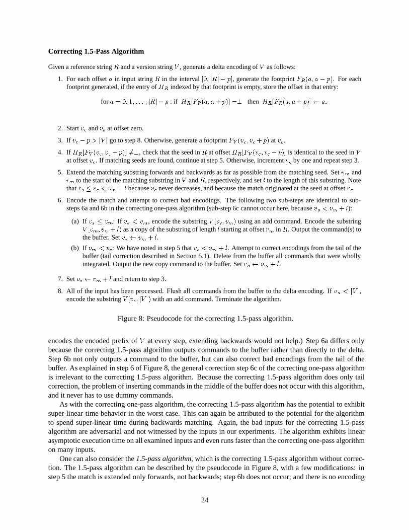
Correcting 1.5-Pass Algorithm

Given a reference string R and a version string V , generate a delta encoding of V as follows:

1. For each offset a in input string R in the interval [0; jRj � p], generate the footprint FR(a; a + p). For eachfootprint generated, if the entry of HR indexed by that footprint is empty, store the offset in that entry:

for a = 0; 1; : : : ; jRj � p : if HR[FR(a; a+ p)] =? then HR[FR(a; a+ p)] a:

2. Start vc and vs at offset zero.

3. If vc + p > jV j go to step 8. Otherwise, generate a footprint FV (vc; vc + p) at vc.

4. If HR[FV (vc; vc + p)] 6=?, check that the seed in R at offset HR[FV (vc; vc + p)] is identical to the seed in Vat offset vc. If matching seeds are found, continue at step 5. Otherwise, increment vc by one and repeat step 3.

5. Extend the matching substring forwards and backwards as far as possible from the matching seed. Set vm andrm to the start of the matching substring in V and R, respectively, and set l to the length of this substring. Notethat vs � vc < vm + l because vc never decreases, and because the match originated at the seed at offset vc.

6. Encode the match and attempt to correct bad encodings. The following two sub-steps are identical to sub-steps 6a and 6b in the correcting one-pass algorithm (sub-step 6c cannot occur here, because vs < vm + l):

(a) If vs � vm: If vs < vm, encode the substring V [vs; vm) using an add command. Encode the substringV [vm; vm+ l) as a copy of the substring of length l starting at offset rm in R. Output the command(s) tothe buffer. Set vs vm + l.

(b) If vm < vs: We have noted in step 5 that vs < vm + l. Attempt to correct encodings from the tail of thebuffer (tail correction described in Section 5.1). Delete from the buffer all commands that were whollyintegrated. Output the new copy command to the buffer. Set vs vm + l.

7. Set vc vm + l and return to step 3.

8. All of the input has been processed. Flush all commands from the buffer to the delta encoding. If vs < jV j,encode the substring V [vs; jV j) with an add command. Terminate the algorithm.

Figure 8: Pseudocode for the correcting 1.5-pass algorithm.

encodes the encoded prefix of V at every step, extending backwards would not help.) Step 6a differs onlybecause the correcting 1.5-pass algorithm outputs commands to the buffer rather than directly to the delta.Step 6b not only outputs a command to the buffer, but can also correct bad encodings from the tail of thebuffer. As explained in step 6 of Figure 8, the general correction step 6c of the correcting one-pass algorithmis irrelevant to the correcting 1.5-pass algorithm. Because the correcting 1.5-pass algorithm does only tailcorrection, the problem of inserting commands in the middle of the buffer does not occur with this algorithm,and it never has to use dummy commands.

As with the correcting one-pass algorithm, the correcting 1.5-pass algorithm has the potential to exhibitsuper-linear time behavior in the worst case. This can again be attributed to the potential for the algorithmto spend super-linear time during backwards matching. Again, the bad inputs for the correcting 1.5-passalgorithm are adversarial and not witnessed by the inputs in our experiments. The algorithm exhibits linearasymptotic execution time on all examined inputs and even runs faster than the correcting one-pass algorithmon many inputs.

One can also consider the 1.5-pass algorithm, which is the correcting 1.5-pass algorithm without correc-tion. The 1.5-pass algorithm can be described by the pseudocode in Figure 8, with a few modifications: instep 5 the match is extended only forwards, not backwards; step 6b does not occur; and there is no encoding

24

lookback buffer, so commands are output directly to the delta. Because the 1.5-pass algorithm does notdo backwards match extension, it runs in linear time in the worst case. Based on our experience with theone-pass and correcting one-pass algorithms, we would expect the 1.5-pass algorithm to run a little fasterthan the correcting 1.5-pass algorithm in practice, but give worse compression.

The correcting 1.5-pass algorithm will likely have poor compression performance when the size of thereference string is much larger than the size of the hash table. In the next section, we explain why this poorperformance occurs, and we describe a technique that essentially reduces the length of the inputs to a lengththat is compatible with the size of the hash table.

8 Handling Arbitrarily Large Input Data

The correcting algorithms have compression limitations when operating on very large inputs. These limita-tions arise as a result of the hash tables these algorithms use becoming overloaded. As increasing the sizeof the hash table is not a scalable solution, we present a method to reduce the amount of information in aninput string to an amount that is compatible with the correcting one-pass and correcting 1.5-pass algorithms.

The compression performance of the correcting 1.5-pass algorithm breaks down when there are manymore offsets than footprint values, that is, when the length of the reference string significantly exceeds thesize of the hash table. When this occurs, many offsets in the reference string have the same footprint valueand must be discarded. As the correcting 1.5-pass algorithm chooses to remember the first offset found foreach footprint, the hash table contains better information about the earlier substrings in the string. For longinputs, information at the end of the string can be sparse, as many footprints will have already occurred. Asthe reference string get larger and larger, the hash table contains less information about the whole string andcompression degrades accordingly.

In contrast, the correcting one-pass algorithm loses the ability to detect “distant” matching data wheninputs grow. The hash tables in the correcting one-pass algorithm always contain the last offset with aparticular footprint. So when inputs are large, the hash table does not cover all previously seen offsets,only the recently seen offsets (the “window into the past”). If matching substrings occur far apart fromsynchronized offsets, the algorithm may miss them, as the “distant” offsets will have been replaced. Thismode of failure is far less severe than that of the correcting 1.5-pass algorithm. Consequently, without theuse of some additional technique to effectively reduce the size of the inputs (such as the technique to bedescribed in this section), the correcting one-pass algorithm is preferable for large inputs.

To address large inputs, we present a technique called checkpointing. The checkpointing techniquedeclares a certain subset of all possible footprints to be checkpoints. The algorithm will then only operateon footprints that are in this checkpoint subset. An algorithm modified with checkpointing will still computea footprint every time that the original algorithm would, but only those footprints that are in the checkpointsubset participate in finding matches. This reduces the number of entries in the hash table(s), and allowsalgorithms to accept longer inputs without the hash table(s) becoming overloaded. For the correcting 1.5-pass algorithm, the expected frequency of checkpoints is chosen so that the hash table contains a goodrepresentation of all sufficiently large regions of the reference string, although not necessarily of all offsets inthe reference string. Because the correcting one-pass algorithm does not need to remember checkpoints overthe entire reference string, but only those in some “window into the past”, the frequency of checkpoints canbe larger for the correcting one-pass algorithm than for the correcting 1.5-pass algorithm; this is discussedin Section 8.2.2.

Checkpointing allows an algorithm to reduce the input size by an arbitrary factor chosen so that thealgorithm exhibits its best performance. We then need to address the issues of selecting checkpoints andintegrating checkpointing into the existing algorithms.

25

8.1 Selecting Checkpoints

Let C be the set of checkpoint values and F be the set of footprint values, so C � F . Say that a seed isa checkpoint seed if the footprint of the seed belongs to the set C of checkpoints. Below we describe amethod for defining the set C, testing whether a given footprint belongs to C, and integrating checkpointinginto differencing algorithms; the only details that the method needs are the number jCj of checkpoints andthe number jFj of footprints. Because there is a one-to-one correspondence between checkpoint valuesand entries in the hash table, we choose jCj based on the amount of memory that we want to use for thehash table. The choice of jFj can depend on the differencing algorithm and the length of the input. Fordefiniteness, we next describe a heuristic for choosing jFj that suits the needs of the correcting 1.5-passalgorithm.

The heuristic is to arrange things so that we expect the number of checkpoint seeds in R to be somechosen fraction of the number of entries in the hash table. For definiteness, we take this fraction to be 1/2(the modifications needed for an arbitrary fraction will be obvious). This fraction is chosen to balance twocompeting goals: (i) to make it unlikely that two different checkpoint seeds that appear in R will collide(have the same footprint), so that the hash table will contain an entry for (almost) all of the checkpoint seedsthat actually appear; and (ii) to utilize a significant fraction of the hash table.

Let L be the length of the string that is to be represented by entries in the hash table; in the present case,L = jRj. In this string, we expect there to be about L � jCj=jFj checkpoint seeds. Using the heuristic thatthis number should be about half the number of hash table entries, we want

L � jCj=jFj � jCj=2; that is, jFj � 2L:

For example, since we are using a modular hash function to generate footprints, jFj equals the modulus q,so q � 2L is used to select q.

We now turn to the process of deciding if a given footprint is a checkpoint. With the goals of efficiencyand simplicity, we take every (jFj=jCj)th footprint to be a checkpoint. Let m be an integer close to jFj=jCj,either m = djFj=jCje or m = bjFj=jCjc. Fix an integer k with 0 � k < m. A given footprint f 2 F is acheckpoint if

f � k (mod m): (4)

(The number of checkpoint values might be slightly smaller or larger than the original goal jCj, dependingon the choice of k and how jFj=jCj is rounded to obtain m.)

To complete the determination of the checkpoints, k must be determined. One possibility is to choosek at random. A better method is to bias the random choice in favor of checkpoints that appear more oftenin V , because this gives a better expected coverage of V by checkpoints. To do this, choose a randomoffset a in V , compute the footprint fa of a, and set k = fa modm. Consider, as a simple example, thatm = 2, there are a large number ` of offsets a in V with fa � 1 modm, and there are a relatively smallnumber s with fa � 0 modm. If k is chosen at random, the expected coverage is E1 = (` + s)=2. If kis chosen by randomly choosing a as above, then the expected coverage is E2 = (`2 + s2)=(` + s). NowE2 � E1 = (` � s)2=(` + s). Because ` + s is a constant (jV j � p+ 1), it follows that E2 � E1 increasesas the square of `� s.

If a footprint f passes the checkpoint test (4), another computation must be done to map f uniquely toan integer i with 0 � i � jFj=m, which will be used to index the hash table. This is easily done by takingi = bf=mc.

Methods other than (4) are possible for defining the set of checkpoints. Assuming that the footprinting(hash) function produces a uniform distribution of footprints over its range [0; jFj), then once we havedecided on the number of footprints and the number jCj of checkpoints, it should not matter what subset

26

of (approximately) jCj footprints is defined to be the set of checkpoints. For example, we could divide theinterval [0; jFj) into disjoint sub-intervals, each containing approximately jCj footprints, and use the biasedrandom method to randomly choose one of these sub-intervals to be the set of checkpoints. This alternativerequires one or two comparisons to test if a footprint is a checkpoint, and a checkpoint is mapped to an indexby one subtraction.

Of course, nothing comes for free: checkpointing has a negative effect on the ability of the algorithmto detect short matching substrings between versions. If an algorithm is to detect and encode a matchingsubstring, one of the seeds of this substring must be a checkpoint seed. Shorter matching substrings willhave fewer checkpoint seeds. If the length of a “short” matching substring is small when compared to thedistance between checkpoint seeds, jFj=jCj on average, the short matching substring will likely be missed,since none of its seeds are checkpoint seeds. On the other hand, for versioned data, we expect highlycorrelated input strings and can expect long matching substrings that contain checkpoint seeds.

8.2 Integrating Checkpoints with Differencing Algorithms

We perform checkpointing in an on-line fashion by testing for checkpoints at the same time that we generatefootprints. For all of our algorithms described above, whenever a footprint f of an offset in string X isgenerated: (i) the algorithm might add or replace an entry at index f in X’s hash table, and (ii) the algorithmchecks if f has a non-null entry in the other string’s hash table. In the algorithm modified with checkpointing,it first tests f (by (4)) to see if it is a checkpoint. If f is not a checkpoint, the algorithm does not perform(i), and it assumes that the test (ii) is false. If f is a checkpoint, f is converted to a hash table index i (byi = bf=mc), and (i) and (ii) are performed using i in place of f .

We also note that the checkpointing technique performs better with algorithms that employ correction.Since an algorithm using checkpointing does not remember offsets whose footprint is not a checkpoint,the algorithm is likely to miss the starting offsets of matching substrings. With correction, however, thealgorithm can still find a matching substring if a checkpoint seed appears anywhere in the substring. Withcorrection, missed starting offsets are handled transparently by backwards matching, and the algorithm findsthe true starts of matching substrings without additional modifications to the algorithm. An algorithm thatuses checkpointing but not correction would fail to copy-encode any portion of a matching substring priorto its first checkpoint seed, as it has no way to encode data prior to its current offset.

8.2.1 Checkpointing and the Correcting 1.5-Pass Algorithm

Checkpointing alleviates the breakdown of the correcting 1.5 pass algorithm operating on large inputs.Using the heuristic described above for choosing jFj, the algorithm can fit an approximation of the contentsof any reference string into its hash table. The argument behind the heuristic is probabilistic, and it ispossible that some of our checkpoints will be very popular (appear at many offsets of R) or not appear atall. A checkpoint that does not appear is a loss, because an entry in the hash table is wasted. A frequentlyappearing checkpoint does not affect the time performance of the algorithm, because we save at most oneoffset for each checkpoint value. For the same reason, this could be detrimental to compression performance,because the offsets appearing in the hash table will be biased toward those near the beginning of R.

8.2.2 Checkpointing and the Correcting One-Pass Algorithm

The correcting one-pass algorithm has problems detecting distant matches when its hash table becomes over-utilized. This is not so much a mode of failure as a property of the algorithm. Applying checkpointing as wedid in the correcting 1.5-pass algorithm allows such distant matches to be detected. In effect, checkpointinggives a “window into the past” that covers a larger portion of the past, but with a more sparse representation.

27

Yet, if the version of the data does not exhibit transpositions, then checkpointing sacrifices the ability todetect short matches and gains no additional benefit.

With the correcting one-pass algorithm, the appropriate frequency of checkpoint seeds depends on thenature of the input data. For data without transpositions, checkpointing can be disregarded. Any policydecision as to the frequency of checkpoints is subject to differing performance, and the nature of the inputdata needs to be considered to formulate such a policy. In our opinion, it can rarely be correct to choose thefrequency as small as was done in the heuristic for the correcting 1.5-pass algorithm, because the correctingone-pass algorithm will then never fill its hash tables and never use its full substring matching capabilities.Frequently occurring checkpoints are not as much of a problem for the correcting one-pass algorithm, be-cause it constantly updates its hash tables (the window into the past). Perhaps a more appropriate heuristicwould be to choose enough checkpoints so that the window into the past covers some fraction of the inputstrings.

9 Experimental Results

We implemented the greedy, one-pass, correcting one-pass, and correcting 1.5-pass algorithms to evaluatetheir compression and running time performance experimentally. Checkpointing was used with the twocorrecting algorithms, but not with the one-pass or greedy algorithms. Experiments were performed on twotypes of input pairs (reference file, version file).4 The first type consisted of two versions of actual files,such as two versions of software. This type generally consisted of pairs where the version file is highlycorrelated with the reference file (an earlier version). On inputs of this type, the two correcting algorithmsachieve better compression than the one-pass algorithm, which confirms our intuition that correction (withcheckpointing) helps compression. Another result is that the compression performance of the correctingalgorithms is close to that of the greedy algorithm that achieves optimal compression. The results alsoindicate that the running times of the new algorithms grow linearly in the size of the files. Although thegreedy algorithm uses more time than the new algorithms, it does not exhibit its worst-case quadratic growthon these highly correlated pairs. To evaluate the time performance of the algorithms on uncorrelated pairs,the algorithms were run on pairs of randomly generated files. Here, the running times of the new algorithmsare linear, while the greedy algorithm does exhibit quadratic time. The experiments verify theoretical resultsabout the algorithms. In particular, the one-pass algorithm runs in linear time, and the greedy algorithm usesquadratic time in the worst case. The experiments also support our assertion that the correcting one-passalgorithm and correcting 1.5-pass algorithms run in linear time, both on actual (correlated) versioned filesand on uncorrelated files.

9.1 Experimental Setup

All algorithms were implemented in the C programming language and were executed on an IBM PowerPCworkstation running the AIX operating system. The workstation was an IBM model 43-P with a 133MHzprocessor and 128 MB of RAM. Files were used as the input strings and all file I/O was performed throughthe local file system. Experiments were conducted out of a warm cache; that is, the input files were alreadyresident in the computer’s memory before measurements were taken. This eliminates the effect of cachingon the measurement of running time. In particular, the first algorithm to run is not penalized for the extratime it spends conducting I/O from disk drives, rather than a cached copy of the data.

Our experiments measure both the time it takes an algorithm to execute and the compression that thealgorithm achieves. Compression is measured as the ratio of the size of the output delta file to the size of the

4In this section, we use the term “file” rather than “string”. A file is given as input to a differencing algorithm by regarding it asa string of bytes.

28

input version file (when defined this way, smaller compression is better). Running time is a measurementof the total execution time of the algorithm. This time includes time the algorithms spend waiting for filesystem I/O operations to complete.

We gave all algorithms 64 kilobytes (KB) of memory for each of their hash tables. However, each entryof the hash table of the greedy algorithm is the head of a linked list containing all offsets with a givenfootprint. Thus, the total space used by the greedy algorithm’s hash table structure is at least jRj, whereasthat of the new algorithms is at most 128KB. The significance of the amount of memory we chose is notin the total memory, but the ratio of the size of the memory to the size of the input. We chose 64KB ofmemory for each hash table so that our input data included files that were more than ten times larger thanthe algorithm’s fixed memory for the hash table used to store information about the seeds appearing in thefile. The two correcting algorithms used a relatively small amount, 4KB, of additional memory for thebuffer (x5), divided into 256 entries of 16 bytes each. Each entry stored the information associated with onecommand; thus, the buffer could hold up to 256 commands at the same time. The length p of seeds was heldfixed at p = 16. (Thus, the delta encodings found by the greedy algorithm are optimal given that matchingsubstrings of length less than p = 16 are not found. To obtain a fair comparison of the new algorithms withthe greedy algorithm, it is reasonable to use the same p for each.)

9.2 Experimental Data

For experimental data, we used multiple versions of application and operating system software distributionsthat are commonly downloaded from the Internet. These distributions include multiple versions of theGNU tools and the BSD operating system distributions, among other data. The files consist of binaryand executable files, source files, and documentation. It does not include image files, multimedia data, ordatabases. We were restricted to distributions of software for which multiple versions were available so thatwe could difference old files against new. In total, our data set consists of over 30,000 files. The average filesize is approximately 180,000 bytes and the maximum file size is 900,000 bytes.

The files we run experiments against were acquired from various Web sites that mirrored GNU and BSDdistributions at various dates during 1996 and 1997. When we found a software distribution for which wealready had an older copy, we would download and build that distribution. Then, we ran scripts that wouldfind files having same path and name in the distribution and would compare them. We discarded all fileswith identical contents and all files not matched, leaving only files that were non-trivially modified betweenversions.5

9.3 Comparisons against Suffix Trees

We do not include a direct comparison against algorithms based on suffix-trees [26], because their spacebounds are unreasonable for our intended applications. However, we do draw some conclusions based onresults presented by Kurtz [16]. A major goal of our differencing algorithms is to compress versions of datamuch larger than the amount of memory available. This cannot be realized using suffix trees. The mostspace-efficient implementation of a suffix tree considered in [16] builds a tree 10 times the size of the input,determined experimentally, and has an analytical bound of 16 times this input size.

When looking at other performance measures, suffix trees are still unattractive. All data in [16] indicatethat suffix trees are substantially less time efficient than our methods. On a machine over twice as fast(300MHz vs. 133MHz) and with more memory (192MB vs. 128MB), suffix trees can be constructed at anaverage rate of 0.4 MB/sec [16] as compared to our algorithms, which produce output at an average rate of0.5 MB/sec or better in our experiments. A delta algorithm based on suffix trees would use even more time,because it has to take a pass over the version file and output a delta after the suffix tree is constructed. Suffix

5These data will be made available by request from randal@cs.jhu.edu.

29

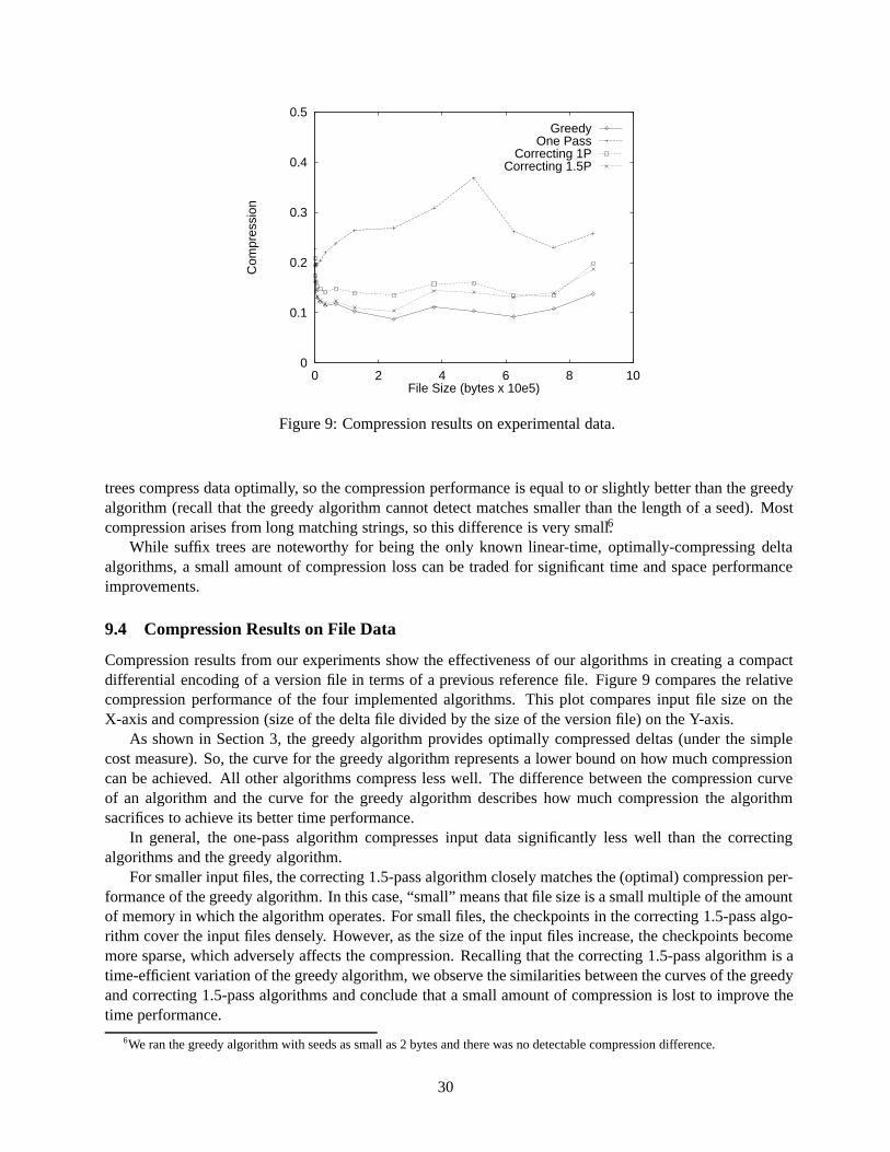
0

0.1

0.2

0.3

0.4

0.5

0 2 4 6 8 10

Com

pres

sion

File Size (bytes x 10e5)

GreedyOne Pass

Correcting 1PCorrecting 1.5P

Figure 9: Compression results on experimental data.

trees compress data optimally, so the compression performance is equal to or slightly better than the greedyalgorithm (recall that the greedy algorithm cannot detect matches smaller than the length of a seed). Mostcompression arises from long matching strings, so this difference is very small.6

While suffix trees are noteworthy for being the only known linear-time, optimally-compressing deltaalgorithms, a small amount of compression loss can be traded for significant time and space performanceimprovements.

9.4 Compression Results on File Data

Compression results from our experiments show the effectiveness of our algorithms in creating a compactdifferential encoding of a version file in terms of a previous reference file. Figure 9 compares the relativecompression performance of the four implemented algorithms. This plot compares input file size on theX-axis and compression (size of the delta file divided by the size of the version file) on the Y-axis.

As shown in Section 3, the greedy algorithm provides optimally compressed deltas (under the simplecost measure). So, the curve for the greedy algorithm represents a lower bound on how much compressioncan be achieved. All other algorithms compress less well. The difference between the compression curveof an algorithm and the curve for the greedy algorithm describes how much compression the algorithmsacrifices to achieve its better time performance.

In general, the one-pass algorithm compresses input data significantly less well than the correctingalgorithms and the greedy algorithm.

For smaller input files, the correcting 1.5-pass algorithm closely matches the (optimal) compression per-formance of the greedy algorithm. In this case, “small” means that file size is a small multiple of the amountof memory in which the algorithm operates. For small files, the checkpoints in the correcting 1.5-pass algo-rithm cover the input files densely. However, as the size of the input files increase, the checkpoints becomemore sparse, which adversely affects the compression. Recalling that the correcting 1.5-pass algorithm is atime-efficient variation of the greedy algorithm, we observe the similarities between the curves of the greedyand correcting 1.5-pass algorithms and conclude that a small amount of compression is lost to improve thetime performance.

6We ran the greedy algorithm with seeds as small as 2 bytes and there was no detectable compression difference.

30

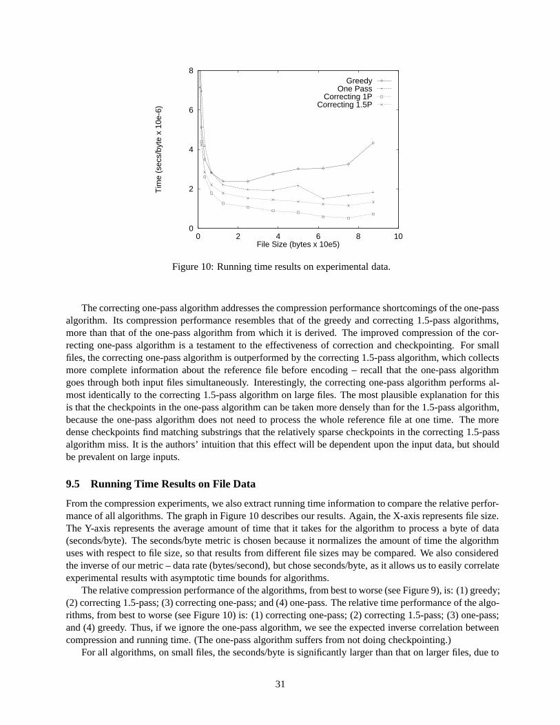
0

2

4

6

8

0 2 4 6 8 10

Tim

e (s

ecs/

byte

x 1

0e-6

)

File Size (bytes x 10e5)

GreedyOne Pass

Correcting 1PCorrecting 1.5P

Figure 10: Running time results on experimental data.

The correcting one-pass algorithm addresses the compression performance shortcomings of the one-passalgorithm. Its compression performance resembles that of the greedy and correcting 1.5-pass algorithms,more than that of the one-pass algorithm from which it is derived. The improved compression of the cor-recting one-pass algorithm is a testament to the effectiveness of correction and checkpointing. For smallfiles, the correcting one-pass algorithm is outperformed by the correcting 1.5-pass algorithm, which collectsmore complete information about the reference file before encoding – recall that the one-pass algorithmgoes through both input files simultaneously. Interestingly, the correcting one-pass algorithm performs al-most identically to the correcting 1.5-pass algorithm on large files. The most plausible explanation for thisis that the checkpoints in the one-pass algorithm can be taken more densely than for the 1.5-pass algorithm,because the one-pass algorithm does not need to process the whole reference file at one time. The moredense checkpoints find matching substrings that the relatively sparse checkpoints in the correcting 1.5-passalgorithm miss. It is the authors’ intuition that this effect will be dependent upon the input data, but shouldbe prevalent on large inputs.

9.5 Running Time Results on File Data

From the compression experiments, we also extract running time information to compare the relative perfor-mance of all algorithms. The graph in Figure 10 describes our results. Again, the X-axis represents file size.The Y-axis represents the average amount of time that it takes for the algorithm to process a byte of data(seconds/byte). The seconds/byte metric is chosen because it normalizes the amount of time the algorithmuses with respect to file size, so that results from different file sizes may be compared. We also consideredthe inverse of our metric – data rate (bytes/second), but chose seconds/byte, as it allows us to easily correlateexperimental results with asymptotic time bounds for algorithms.

The relative compression performance of the algorithms, from best to worse (see Figure 9), is: (1) greedy;(2) correcting 1.5-pass; (3) correcting one-pass; and (4) one-pass. The relative time performance of the algo-rithms, from best to worse (see Figure 10) is: (1) correcting one-pass; (2) correcting 1.5-pass; (3) one-pass;and (4) greedy. Thus, if we ignore the one-pass algorithm, we see the expected inverse correlation betweencompression and running time. (The one-pass algorithm suffers from not doing checkpointing.)

For all algorithms, on small files, the seconds/byte is significantly larger than that on larger files, due to

31

certain start-up costs such as program load, initializing data structures, and memory allocation. For largerinputs, the total time over which an algorithm runs increases, so the start-up cost is amortized over morebytes.

The running time results show that the one-pass algorithm and the two correcting algorithms proceedthrough data at roughly a constant rate for files of all sizes. This represents linear asymptotic growth inthe algorithms’ times. Small variations in seconds/byte arise due to differences in the experimental data.The one-pass algorithm proceeds through data at different rates depending upon whether it is searching formatching strings or encoding matching data between versions (Section 4). So the actual time performancevaries depending upon the compressibility of data and type of changes that occur.

We first consider the effect of correction by comparing the one-pass algorithm with the correcting al-gorithms. For larger files, both correcting algorithms use less time than the one-pass algorithm. Becausethe correcting algorithms use the checkpointing technique to reduce the number of offsets that they examineto find and encode matches, the seconds/byte decreases as files grow. That is, the larger the file, the largerthe checkpoint interval, and the less dense the checkpoints in the file. For large files, checkpointing domi-nates performance, and the correcting algorithms outperform the one-pass algorithm. For small files, wherecheckpointing is not a factor, the performance of the one-pass algorithm is inferior to the performance ofother algorithms because it produces significantly larger delta files. Poor compression performance causesthe algorithm to perform significantly more I/O, increasing the running time.

Comparing now the correcting one-pass and the correcting 1.5-pass algorithms, we see that their runningtimes are very similar, with the correcting one-pass algorithm having slightly faster running time than thecorrecting 1.5-pass algorithm at all points. The correcting one-pass algorithm has the advantage of beingable to go through both files at the same time, as opposed to examining the whole reference file before en-coding the version file. The slight time advantages of the correcting one-pass algorithm should be comparedagainst the slight compression advantages of the correcting 1.5-pass algorithm. Neither algorithm standsout as clearly superior; rather, the correcting one-pass algorithm has advantages for large inputs where itsrunning time is superior, while the correcting 1.5-pass algorithm has compression advantages for small andmoderate sized inputs.

The greedy algorithm has running time comparable to that of other algorithms for very small files, but forlarger file sizes its running time is significantly worse. The greedy algorithm displays a moderate increase inseconds/byte running time as file size increases. However, the algorithm does not display a linear increasein seconds/byte running time that would result from quadratic growth of time versus file size. The greedyalgorithm does not display quadratic time behavior here, because the experimental data is so compressible.For illustration, consider the greedy algorithm differencing two files that are identical. The algorithm buildsits data structures in linear time7, finds a matching seed at the first offset of each file, extends this match tothe end of both files, and encodes the match with a single copy command. This all occurs in O(n) time.

9.6 Running Time Results on Uncorrelated Versions

Almost all the file data used in our experiments shared the trait of similarity between versions. The versionfiles were highly compressible using differencing algorithms, which indicates that they share many commonsubstrings with their corresponding reference versions. To better understand the time performance of thefour algorithms, and explore worst case behavior, we also ran the algorithms against uncorrelated files, twofiles that are likely to share only very short common substrings. We tested differencing on pairs of files thatwere roughly the same length, but whose bytes were random with respect to each other. To create uncor-

7Our implementation of the greedy algorithm is based on an algorithm in the literature [20] that constructs its hash table usingtime in (n2). We modified the algorithm to construct the hash table in O(n) time. This modification in no way changes themanner in which the algorithm finds and encodes matching substrings, so it does not affect the proof that it compresses optimally.This change makes for a more equitable comparison of a greedy algorithm with other algorithms.

32

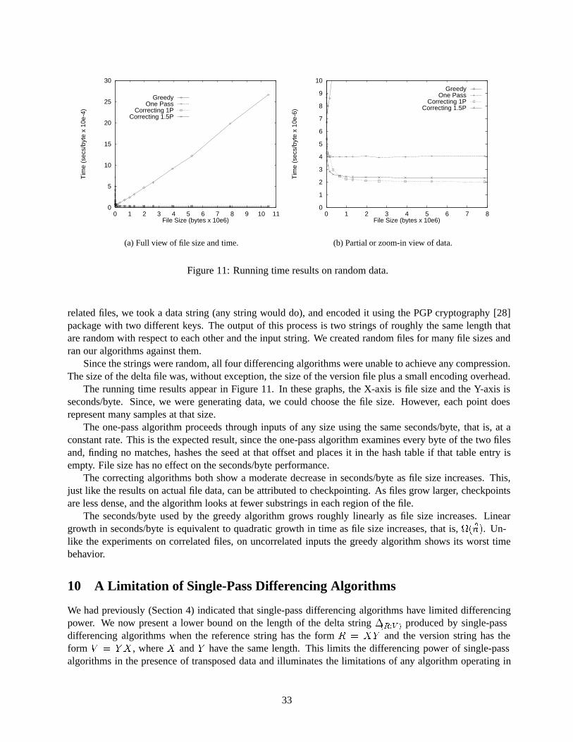
0

5

10

15

20

25

30

0 1 2 3 4 5 6 7 8 9 10 11

Tim

e (s

ecs/

byte

x 1

0e-4

)

File Size (bytes x 10e6)

GreedyOne Pass

Correcting 1PCorrecting 1.5P

(a) Full view of file size and time.

0

1

2

3

4

5

6

7

8

9

10

0 1 2 3 4 5 6 7 8

Tim

e (s

ecs/

byte

x 1

0e-6

)

File Size (bytes x 10e6)

GreedyOne Pass

Correcting 1PCorrecting 1.5P

(b) Partial or zoom-in view of data.

Figure 11: Running time results on random data.

related files, we took a data string (any string would do), and encoded it using the PGP cryptography [28]package with two different keys. The output of this process is two strings of roughly the same length thatare random with respect to each other and the input string. We created random files for many file sizes andran our algorithms against them.

Since the strings were random, all four differencing algorithms were unable to achieve any compression.The size of the delta file was, without exception, the size of the version file plus a small encoding overhead.

The running time results appear in Figure 11. In these graphs, the X-axis is file size and the Y-axis isseconds/byte. Since, we were generating data, we could choose the file size. However, each point doesrepresent many samples at that size.

The one-pass algorithm proceeds through inputs of any size using the same seconds/byte, that is, at aconstant rate. This is the expected result, since the one-pass algorithm examines every byte of the two filesand, finding no matches, hashes the seed at that offset and places it in the hash table if that table entry isempty. File size has no effect on the seconds/byte performance.

The correcting algorithms both show a moderate decrease in seconds/byte as file size increases. This,just like the results on actual file data, can be attributed to checkpointing. As files grow larger, checkpointsare less dense, and the algorithm looks at fewer substrings in each region of the file.

The seconds/byte used by the greedy algorithm grows roughly linearly as file size increases. Lineargrowth in seconds/byte is equivalent to quadratic growth in time as file size increases, that is, (n2). Un-like the experiments on correlated files, on uncorrelated inputs the greedy algorithm shows its worst timebehavior.

10 A Limitation of Single-Pass Differencing Algorithms

We had previously (Section 4) indicated that single-pass differencing algorithms have limited differencingpower. We now present a lower bound on the length of the delta string �(R:V ) produced by single-passdifferencing algorithms when the reference string has the form R = XY and the version string has theform V = Y X , where X and Y have the same length. This limits the differencing power of single-passalgorithms in the presence of transposed data and illuminates the limitations of any algorithm operating in

33

single pass over the input.The definition of “single-pass” in this section is strict: each string is scanned by one pointer that can

only move from the beginning of the string to the end; no random-access or reversal is allowed. This is aconsiderably more stringent restriction than the one used in the one-pass algorithm, because the one-passalgorithm can use random-access in its attempts to find matching substrings. The inputs R and V and theoutput delta are all binary strings. If n is the length of R (this is a different definition of n than the one usedpreviously) and the algorithm has m bits of memory, the lower bound is n=2 �m � O(logn). As shownbelow, this lower bound is optimal to within an additive O(logn) term. In the strongest version of the result,the algorithm can be probabilistic, X and Y are random strings of length n=2, and the lower bound is onthe expected length of �(R:V ). The lower bound holds for any encoding method having the property that Vcan be recovered from R and �(R:V ). One such method is the one described in Section 2.1.1, where V isencoded as a sequence of added substrings and substrings copied from R.

10.1 Encoding Methods

Let f0; 1g� denote the set of all binary strings, and let f0; 1gn denote the set of binary strings of length n.All logarithms are to the base 2.

An encoding method is a function � that maps each pair R and V of binary strings to a nonempty set�(R;V ) of binary strings. Each string in �(R;V ) is an encoding of V with respect to R. In order thatV be recoverable from R and any string in �(R;V ), we require that, for all R;V; V0, if V 6= V 0 then�(R;V ) \ �(R;V 0) = ;.

10.2 Model of Computation

A single-pass differencing algorithm is performed by an automaton, that we call a single-pass automaton,having two input tapes, a finite-state control, and a mechanism for producing an output string (describedbelow). A few words should be said about the assumption of a finite-state control, even though the inputstrings could be arbitrarily large. In the definitions given next and in the statements of the results, we assumethat the length of each input is some fixed (but arbitrary) even number n. The lower bound on the length ofthe output is stated in terms of n and the number of bits of memory in the finite state control, that is, the logof the number of states. Alternatively, the results could be stated in an “asymptotic” way, where the size ofmemory increases as some function of n. Stating the results as we do has the advantage that the results holdin a non-uniform model, where we can use a different differencing algorithm for each length n of the inputs;again the size of memory can increase as n increases. Because we are proving lower bounds on the lengthof the output, our results can only become stronger by using a more general model.

We first describe this type of automaton informally, and then give a more precise definition. One inputtape (tape 1) holds the reference string R, and the other (tape 2) holds the version string V ; each stringis followed by an end-of-string character denoted $. Each input tape is scanned by a single reading head,which is initially positioned on the leftmost bit of the string. Each head on an input tape can move onlyfrom left to right. Typically, the output string of a finite-state machine is produced incrementally, by issuingthe symbols of the string from left to right. We can use a more general type of output mechanism, whichpermits incremental changes other than appending a symbol at the end. For example, this mechanism allowsa certain number of symbols to be erased from the end. In more detail, the finite-state control can issueoutput actions. Each output action is a function from binary strings to binary strings. Initially the outputstring is the empty string. If the output action � is issued when the output string is w, the output stringis changed to �(w). Without some restriction on the output actions, this model can compute any functionf(R; V ) (e.g., the function computed by a perfect differencing algorithm): the automaton first copies theinputs R and V to the output string and then issues an output action that has the effect of applying f to R

34

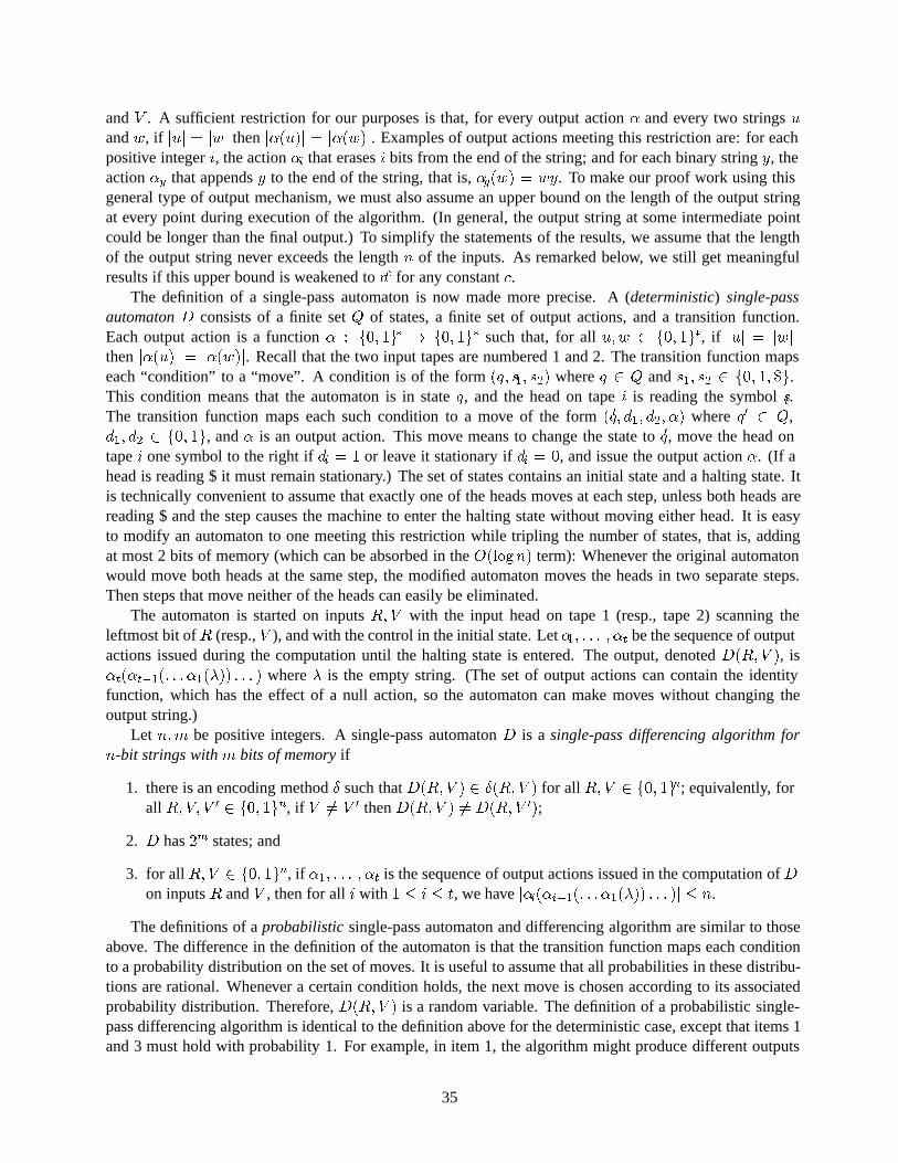
and V . A sufficient restriction for our purposes is that, for every output action � and every two strings uand w, if juj = jwj then j�(u)j = j�(w)j. Examples of output actions meeting this restriction are: for eachpositive integer i, the action �i that erases i bits from the end of the string; and for each binary string y, theaction �y that appends y to the end of the string, that is, �y(w) = wy. To make our proof work using thisgeneral type of output mechanism, we must also assume an upper bound on the length of the output stringat every point during execution of the algorithm. (In general, the output string at some intermediate pointcould be longer than the final output.) To simplify the statements of the results, we assume that the lengthof the output string never exceeds the length n of the inputs. As remarked below, we still get meaningfulresults if this upper bound is weakened to nc for any constant c.

The definition of a single-pass automaton is now made more precise. A (deterministic) single-passautomaton D consists of a finite set Q of states, a finite set of output actions, and a transition function.Each output action is a function � : f0; 1g� ! f0; 1g� such that, for all u;w 2 f0; 1g�, if juj = jwjthen j�(u)j = j�(w)j. Recall that the two input tapes are numbered 1 and 2. The transition function mapseach “condition” to a “move”. A condition is of the form (q; s1; s2) where q 2 Q and s1; s2 2 f0; 1; $g.This condition means that the automaton is in state q, and the head on tape i is reading the symbol si.The transition function maps each such condition to a move of the form (q0; d1; d2; �) where q0 2 Q,d1; d2 2 f0; 1g, and � is an output action. This move means to change the state to q0, move the head ontape i one symbol to the right if di = 1 or leave it stationary if di = 0, and issue the output action �. (If ahead is reading $ it must remain stationary.) The set of states contains an initial state and a halting state. Itis technically convenient to assume that exactly one of the heads moves at each step, unless both heads arereading $ and the step causes the machine to enter the halting state without moving either head. It is easyto modify an automaton to one meeting this restriction while tripling the number of states, that is, addingat most 2 bits of memory (which can be absorbed in the O(logn) term): Whenever the original automatonwould move both heads at the same step, the modified automaton moves the heads in two separate steps.Then steps that move neither of the heads can easily be eliminated.

The automaton is started on inputs R;V with the input head on tape 1 (resp., tape 2) scanning theleftmost bit of R (resp., V ), and with the control in the initial state. Let �1; : : : ; �t be the sequence of outputactions issued during the computation until the halting state is entered. The output, denoted D(R;V ), is�t(�t�1(: : : �1(�)) : : : ) where � is the empty string. (The set of output actions can contain the identityfunction, which has the effect of a null action, so the automaton can make moves without changing theoutput string.)

Let n;m be positive integers. A single-pass automaton D is a single-pass differencing algorithm forn-bit strings with m bits of memory if

1. there is an encoding method � such that D(R;V ) 2 �(R; V ) for all R; V 2 f0; 1gn; equivalently, forall R;V; V 0 2 f0; 1gn, if V 6= V 0 then D(R;V ) 6= D(R;V 0);

2. D has 2m states; and

3. for all R;V 2 f0; 1gn, if �1; : : : ; �t is the sequence of output actions issued in the computation of Don inputs R and V , then for all i with 1 � i � t, we have j�i(�i�1(: : : �1(�)) : : : )j � n.

The definitions of a probabilistic single-pass automaton and differencing algorithm are similar to thoseabove. The difference in the definition of the automaton is that the transition function maps each conditionto a probability distribution on the set of moves. It is useful to assume that all probabilities in these distribu-tions are rational. Whenever a certain condition holds, the next move is chosen according to its associatedprobability distribution. Therefore, D(R;V ) is a random variable. The definition of a probabilistic single-pass differencing algorithm is identical to the definition above for the deterministic case, except that items 1and 3 must hold with probability 1. For example, in item 1, the algorithm might produce different outputs

35

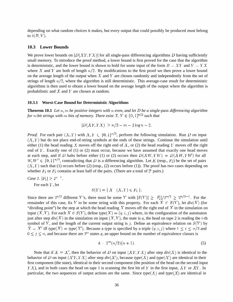
depending on what random choices it makes, but every output that could possibly be produced must belongto �(R; V ).

10.3 Lower Bounds

We prove lower bounds on jD(XY; YX)j for all single-pass differencing algorithms D having sufficientlysmall memory. To introduce the proof method, a lower bound is first proved for the case that the algorithmis deterministic, and the lower bound is shown to hold for some input of the form R = XY and V = Y Xwhere X and Y are both of length n=2. By modifications to the first proof we then prove a lower boundon the average length of the output when X and Y are chosen randomly and independently from the set ofstrings of length n=2, where the algorithm is still deterministic. This average-case result for deterministicalgorithms is then used to obtain a lower bound on the average length of the output where the algorithm isprobabilistic and X and Y are chosen at random.

10.3.1 Worst-Case Bound for Deterministic Algorithms

Theorem 10.1 Let n;m be positive integers with n even, and let D be a single-pass differencing algorithmfor n-bit strings with m bits of memory. There exist X;Y 2 f0; 1gn=2 such that

jD(XY; YX)j � n=2�m � 2 logn� 2:

Proof. For each pair (X;Y ) with X;Y 2 f0; 1gn=2, perform the following simulation. Run D on input(X;Y ) but do not place end-of-string symbols at the ends of these strings. Continue the simulation untileither (1) the head reading X moves off the right end of X , or (2) the head reading Y moves off the rightend of Y . Exactly one of (1) or (2) must occur, because we have assumed that exactly one head movesat each step, and if D halts before either (1) or (2) occurs then D(XW;YW ) = D(XW;YW0) for allW;W 0 2 f0; 1gn=2, contradicting that D is a differencing algorithm. Let F1 (resp., F2) be the set of pairs(X;Y ) such that (1) occurs before (2) (resp., (2) occurs before (1)). The proof has two cases depending onwhether F1 or F2 contains at least half of the pairs. (There are a total of 2n pairs.)

Case 1. jF1j � 2n�1.

For each Y , letS(Y ) = fX j (X;Y ) 2 F1 g:

Since there are 2n=2 different Y ’s, there must be some Y with jS(Y )j � jF1j=2n=2 � 2n=2�1. For theremainder of this case, fix Y to be some string with this property. For each X 2 S(Y ), let div(X) (for“dividing point”) be the step at which the head reading X moves off the right end of X in the simulation oninput (X;Y ). For each X 2 S(Y ), define type(X) = (q; i; j) where, in the configuration of the automatonjust after step div(X) in the simulation on input (X;Y ), the state is q, the head on tape 2 is reading the i-thsymbol of Y , and the length of the current output string is j. Define an equivalence relation on S(Y ) byX � X 0 iff type(X) = type(X0). Because a type is specified by a triple (q; i; j) where 1 � i � n=2 and0 � j � n, and because there are 2m states q, an upper bound on the number of equivalence classes is

k = 2m(n=2)(n+ 1): (5)

Note that if X � X0, then the behavior of D on input (XY; Y X) after step div(X) is identical to thebehavior of D on input (X0Y; Y X) after step div(X0), because type(X) and type(X0) are identical in theirfirst component (the state), identical in their second component (the position of the head on the second inputY X), and in both cases the head on tape 1 is scanning the first bit of Y in the first input, XY or X0Y . Inparticular, the two sequences of output actions are the same. Since type(X) and type(X0) are identical in

36

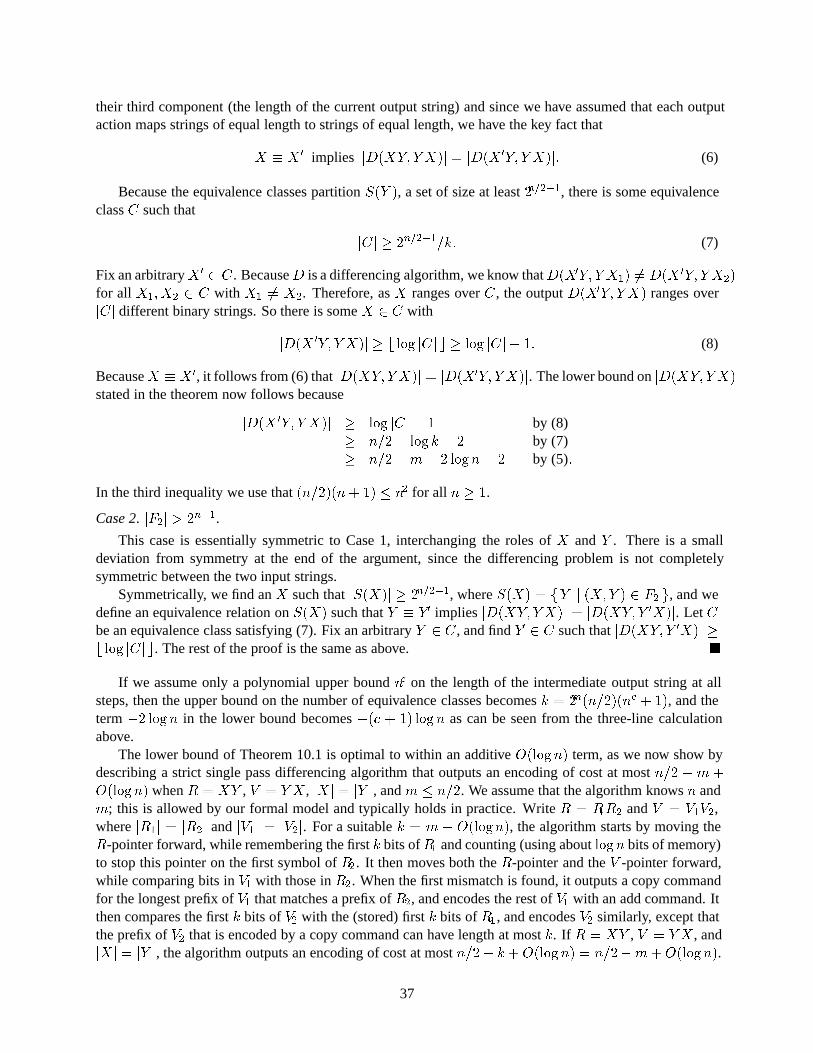
their third component (the length of the current output string) and since we have assumed that each outputaction maps strings of equal length to strings of equal length, we have the key fact that

X � X 0 implies jD(XY; YX)j = jD(X0Y; Y X)j: (6)

Because the equivalence classes partition S(Y ), a set of size at least 2n=2�1, there is some equivalenceclass C such that

jCj � 2n=2�1=k: (7)

Fix an arbitrary X0 2 C . BecauseD is a differencing algorithm, we know thatD(X0Y; Y X1) 6= D(X 0Y; Y X2)for all X1;X2 2 C with X1 6= X2. Therefore, as X ranges over C , the output D(X0Y; Y X) ranges overjCj different binary strings. So there is some X 2 C with

jD(X 0Y; Y X)j � b log jCj c � log jCj � 1: (8)

BecauseX � X0, it follows from (6) that jD(XY; YX)j = jD(X0Y; Y X)j. The lower bound on jD(XY; YX)jstated in the theorem now follows because

jD(X 0Y; Y X)j � log jCj � 1 by (8)� n=2� logk � 2 by (7)� n=2�m � 2 logn� 2 by (5):

In the third inequality we use that (n=2)(n+ 1) � n2 for all n � 1.

Case 2. jF2j > 2n�1.

This case is essentially symmetric to Case 1, interchanging the roles of X and Y . There is a smalldeviation from symmetry at the end of the argument, since the differencing problem is not completelysymmetric between the two input strings.

Symmetrically, we find an X such that jS(X)j � 2n=2�1, where S(X) = fY j (X;Y ) 2 F2 g, and wedefine an equivalence relation on S(X) such that Y � Y0 implies jD(XY; YX)j = jD(XY; Y 0X)j. Let Cbe an equivalence class satisfying (7). Fix an arbitrary Y 2 C , and find Y0 2 C such that jD(XY; Y 0X)j �b log jCj c. The rest of the proof is the same as above. �

If we assume only a polynomial upper bound nc on the length of the intermediate output string at allsteps, then the upper bound on the number of equivalence classes becomes k = 2m(n=2)(nc + 1), and theterm �2 logn in the lower bound becomes �(c + 1) logn as can be seen from the three-line calculationabove.

The lower bound of Theorem 10.1 is optimal to within an additive O(logn) term, as we now show bydescribing a strict single pass differencing algorithm that outputs an encoding of cost at most n=2 � m +O(logn) when R = XY , V = Y X , jXj = jY j, and m � n=2. We assume that the algorithm knows n andm; this is allowed by our formal model and typically holds in practice. Write R = R1R2 and V = V1V2,where jR1j = jR2j and jV1j = jV2j. For a suitable k = m � O(logn), the algorithm starts by moving theR-pointer forward, while remembering the first k bits ofR1 and counting (using about logn bits of memory)to stop this pointer on the first symbol of R2. It then moves both the R-pointer and the V -pointer forward,while comparing bits in V1 with those in R2. When the first mismatch is found, it outputs a copy commandfor the longest prefix of V1 that matches a prefix of R2, and encodes the rest of V1 with an add command. Itthen compares the first k bits of V2 with the (stored) first k bits of R1, and encodes V2 similarly, except thatthe prefix of V2 that is encoded by a copy command can have length at most k. If R = XY , V = Y X , andjXj = jY j, the algorithm outputs an encoding of cost at most n=2� k +O(logn) = n=2�m+O(logn).

37

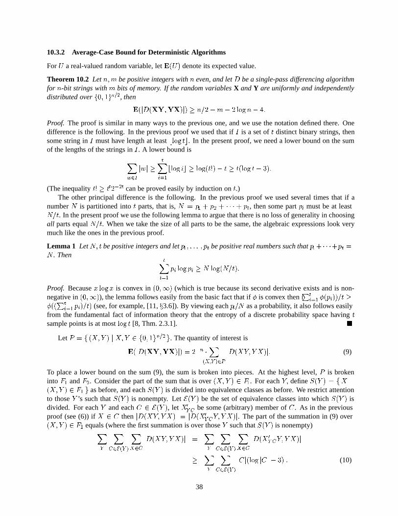
10.3.2 Average-Case Bound for Deterministic Algorithms

For U a real-valued random variable, let E(U) denote its expected value.

Theorem 10.2 Let n;m be positive integers with n even, and let D be a single-pass differencing algorithmfor n-bit strings with m bits of memory. If the random variables X and Y are uniformly and independentlydistributed over f0; 1gn=2, then

E(jD(XY;YX)j) � n=2�m � 2 logn� 4:

Proof. The proof is similar in many ways to the previous one, and we use the notation defined there. Onedifference is the following. In the previous proof we used that if I is a set of t distinct binary strings, thensome string in I must have length at least blog tc. In the present proof, we need a lower bound on the sumof the lengths of the strings in I . A lower bound is

Xw2I

jwj �tX

i=1

blog ic � log(t!)� t � t(log t� 3):

(The inequality t! � tt2�2t can be proved easily by induction on t.)The other principal difference is the following. In the previous proof we used several times that if a

number N is partitioned into t parts, that is, N = p1 + p2 + � � � + pt, then some part pi must be at leastN=t. In the present proof we use the following lemma to argue that there is no loss of generality in choosingall parts equal N=t. When we take the size of all parts to be the same, the algebraic expressions look verymuch like the ones in the previous proof.

Lemma 1 Let N; t be positive integers and let p1; : : : ; pt be positive real numbers such that p1+ � � �+pt =N . Then

tXi=1

pi log pi � N log(N=t):

Proof. Because x logx is convex in (0;1) (which is true because its second derivative exists and is non-negative in (0;1)), the lemma follows easily from the basic fact that if � is convex then (

Pti=1 �(pi))=t �

�((Pt

i=1 pi)=t) (see, for example, [11, x3.6]). By viewing each pi=N as a probability, it also follows easilyfrom the fundamental fact of information theory that the entropy of a discrete probability space having tsample points is at most log t [8, Thm. 2.3.1]. �

Let P = f (X;Y ) j X;Y 2 f0; 1gn=2 g. The quantity of interest is

E(jD(XY;YX)j) = 2�n �X

(X;Y )2P

jD(XY; YX)j: (9)

To place a lower bound on the sum (9), the sum is broken into pieces. At the highest level, P is brokeninto F1 and F2. Consider the part of the sum that is over (X;Y ) 2 F1. For each Y; define S(Y ) = fX j(X;Y ) 2 F1 g as before, and each S(Y ) is divided into equivalence classes as before. We restrict attentionto those Y ’s such that S(Y ) is nonempty. Let E(Y ) be the set of equivalence classes into which S(Y ) isdivided. For each Y and each C 2 E(Y ), let X0

Y C be some (arbitrary) member of C . As in the previousproof (see (6)) if X 2 C then jD(XY; YX)j = jD(X0

Y CY; Y X)j. The part of the summation in (9) over(X;Y ) 2 F1 equals (where the first summation is over those Y such that S(Y ) is nonempty)X

Y

XC2E(Y )

XX2C

jD(XY; YX)j =XY

XC2E(Y )

XX2C

jD(X 0Y CY; Y X)j

�XY

XC2E(Y )

jCj(log jCj � 3) : (10)

38

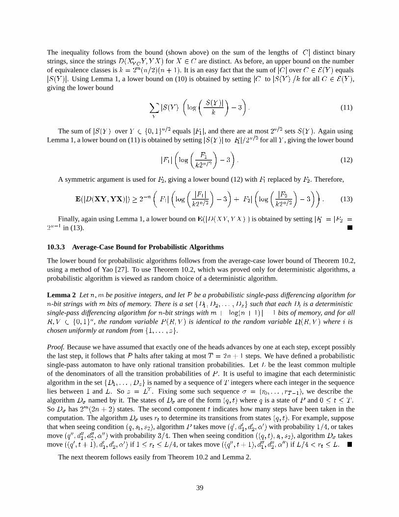
The inequality follows from the bound (shown above) on the sum of the lengths of jCj distinct binarystrings, since the strings D(X0

Y CY; Y X) for X 2 C are distinct. As before, an upper bound on the numberof equivalence classes is k = 2m(n=2)(n+ 1). It is an easy fact that the sum of jCj over C 2 E(Y ) equalsjS(Y )j. Using Lemma 1, a lower bound on (10) is obtained by setting jCj to jS(Y )j=k for all C 2 E(Y ),giving the lower bound

XY

jS(Y )j

�log

�jS(Y )j

k

�� 3

�: (11)

The sum of jS(Y )j over Y 2 f0; 1gn=2 equals jF1j, and there are at most 2n=2 sets S(Y ). Again usingLemma 1, a lower bound on (11) is obtained by setting jS(Y )j to jF1j=2n=2 for all Y , giving the lower bound

jF1j

�log

�jF1j

k2n=2

�� 3

�: (12)

A symmetric argument is used for F2, giving a lower bound (12) with F1 replaced by F2. Therefore,

E(jD(XY;YX)j) � 2�n�jF1j

�log

�jF1j

k2n=2

�� 3

�+ jF2j

�log

�jF2j

k2n=2

�� 3

��: (13)

Finally, again using Lemma 1, a lower bound on E(jD(XY; Y X)j) is obtained by setting jF1j = jF2j =2n�1 in (13). �

10.3.3 Average-Case Bound for Probabilistic Algorithms

The lower bound for probabilistic algorithms follows from the average-case lower bound of Theorem 10.2,using a method of Yao [27]. To use Theorem 10.2, which was proved only for deterministic algorithms, aprobabilistic algorithm is viewed as random choice of a deterministic algorithm.

Lemma 2 Let n;m be positive integers, and let P be a probabilistic single-pass differencing algorithm forn-bit strings with m bits of memory. There is a set fD1;D2; : : : ;Dzg such that each Di is a deterministicsingle-pass differencing algorithm for n-bit strings with m + dlog(n+ 1)e + 1 bits of memory, and for allR; V 2 f0; 1gn, the random variable P (R;V ) is identical to the random variable Di(R;V ) where i ischosen uniformly at random from f1; : : : ; zg.

Proof. Because we have assumed that exactly one of the heads advances by one at each step, except possiblythe last step, it follows that P halts after taking at most T = 2n+ 1 steps. We have defined a probabilisticsingle-pass automaton to have only rational transition probabilities. Let L be the least common multipleof the denominators of all the transition probabilities of P . It is useful to imagine that each deterministicalgorithm in the set fD1; : : : ;Dzg is named by a sequence of T integers where each integer in the sequencelies between 1 and L. So z = LT . Fixing some such sequence � = (r0; : : : ; rT�1), we describe thealgorithm D� named by it. The states of D� are of the form (q; t) where q is a state of P and 0 � t � T .So D� has 2m(2n + 2) states. The second component t indicates how many steps have been taken in thecomputation. The algorithm D� uses rt to determine its transitions from states (q; t). For example, supposethat when seeing condition (q; s1; s2), algorithm P takes move (q0; d01; d

02; �

0) with probability 1=4, or takesmove (q00; d001 ; d

002; �

00) with probability 3=4. Then when seeing condition ((q; t); s1; s2), algorithm D� takesmove ((q0; t+ 1); d01; d

02; �

0) if 1 � rt � L=4, or takes move ((q00; t+ 1); d001; d002; �

00) if L=4 < rt � L. �

The next theorem follows easily from Theorem 10.2 and Lemma 2.

39

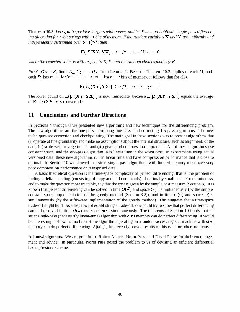
Theorem 10.3 Let n;m be positive integers with n even, and let P be a probabilistic single-pass differenc-ing algorithm for n-bit strings with m bits of memory. If the random variables X and Y are uniformly andindependently distributed over f0; 1gn=2, then

E(jP (XY;YX)j) � n=2�m � 3 logn� 6

where the expected value is with respect to X, Y, and the random choices made by P .

Proof. Given P , find fD1;D2; : : : ;Dzg from Lemma 2. Because Theorem 10.2 applies to each Di, andeach Di has m + dlog(n+ 1)e+ 1 � m + logn+ 2 bits of memory, it follows that for all i,

E(jDi(XY;YX)j) � n=2�m � 3 logn� 6:

The lower bound on E(jP (XY;YX)j) is now immediate, because E(jP (XY;YX)j) equals the averageof E(jDi(XY;YX)j) over all i.

11 Conclusions and Further Directions

In Sections 4 through 8 we presented new algorithms and new techniques for the differencing problem.The new algorithms are the one-pass, correcting one-pass, and correcting 1.5-pass algorithms. The newtechniques are correction and checkpointing. The main goal in these sections was to present algorithms that(i) operate at fine granularity and make no assumptions about the internal structure, such as alignment, of thedata; (ii) scale well to large inputs; and (iii) give good compression in practice. All of these algorithms useconstant space, and the one-pass algorithm uses linear time in the worst case. In experiments using actualversioned data, these new algorithms run in linear time and have compression performance that is close tooptimal. In Section 10 we showed that strict single-pass algorithms with limited memory must have verypoor compression performance on transposed data.

A basic theoretical question is the time-space complexity of perfect differencing, that is, the problem offinding a delta encoding (consisting of copy and add commands) of optimally small cost. For definiteness,and to make the question more tractable, say that the cost is given by the simple cost measure (Section 3). It isknown that perfect differencing can be solved in time O(n2) and space O(1) simultaneously (by the simpleconstant-space implementation of the greedy method (Section 3.2)), and in time O(n) and space O(n)simultaneously (by the suffix-tree implementation of the greedy method). This suggests that a time-spacetrade-off might hold. As a step toward establishing a trade-off, one could try to show that perfect differencingcannot be solved in time O(n) and space o(n) simultaneously. The theorems of Section 10 imply that nostrict single-pass (necessarily linear-time) algorithm with o(n) memory can do perfect differencing. It wouldbe interesting to show that no linear-time algorithm operating on a random-access register machine with o(n)memory can do perfect differencing. Ajtai [1] has recently proved results of this type for other problems.

Acknowledgments. We are grateful to Robert Morris, Norm Pass, and David Pease for their encourage-ment and advice. In particular, Norm Pass posed the problem to us of devising an efficient differentialbackup/restore scheme.

40

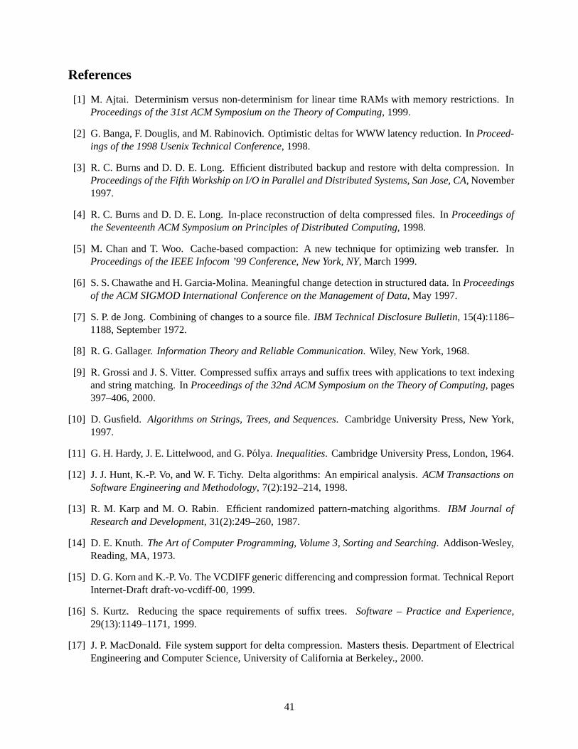
References

[1] M. Ajtai. Determinism versus non-determinism for linear time RAMs with memory restrictions. InProceedings of the 31st ACM Symposium on the Theory of Computing, 1999.

[2] G. Banga, F. Douglis, and M. Rabinovich. Optimistic deltas for WWW latency reduction. In Proceed-ings of the 1998 Usenix Technical Conference, 1998.

[3] R. C. Burns and D. D. E. Long. Efficient distributed backup and restore with delta compression. InProceedings of the Fifth Workship on I/O in Parallel and Distributed Systems, San Jose, CA, November1997.

[4] R. C. Burns and D. D. E. Long. In-place reconstruction of delta compressed files. In Proceedings ofthe Seventeenth ACM Symposium on Principles of Distributed Computing, 1998.

[5] M. Chan and T. Woo. Cache-based compaction: A new technique for optimizing web transfer. InProceedings of the IEEE Infocom ’99 Conference, New York, NY, March 1999.

[6] S. S. Chawathe and H. Garcia-Molina. Meaningful change detection in structured data. In Proceedingsof the ACM SIGMOD International Conference on the Management of Data, May 1997.

[7] S. P. de Jong. Combining of changes to a source file. IBM Technical Disclosure Bulletin, 15(4):1186–1188, September 1972.

[8] R. G. Gallager. Information Theory and Reliable Communication. Wiley, New York, 1968.

[9] R. Grossi and J. S. Vitter. Compressed suffix arrays and suffix trees with applications to text indexingand string matching. In Proceedings of the 32nd ACM Symposium on the Theory of Computing, pages397–406, 2000.

[10] D. Gusfield. Algorithms on Strings, Trees, and Sequences. Cambridge University Press, New York,1997.

[11] G. H. Hardy, J. E. Littelwood, and G. Polya. Inequalities. Cambridge University Press, London, 1964.

[12] J. J. Hunt, K.-P. Vo, and W. F. Tichy. Delta algorithms: An empirical analysis. ACM Transactions onSoftware Engineering and Methodology, 7(2):192–214, 1998.

[13] R. M. Karp and M. O. Rabin. Efficient randomized pattern-matching algorithms. IBM Journal ofResearch and Development, 31(2):249–260, 1987.

[14] D. E. Knuth. The Art of Computer Programming, Volume 3, Sorting and Searching. Addison-Wesley,Reading, MA, 1973.

[15] D. G. Korn and K.-P. Vo. The VCDIFF generic differencing and compression format. Technical ReportInternet-Draft draft-vo-vcdiff-00, 1999.

[16] S. Kurtz. Reducing the space requirements of suffix trees. Software – Practice and Experience,29(13):1149–1171, 1999.

[17] J. P. MacDonald. File system support for delta compression. Masters thesis. Department of ElectricalEngineering and Computer Science, University of California at Berkeley., 2000.

41

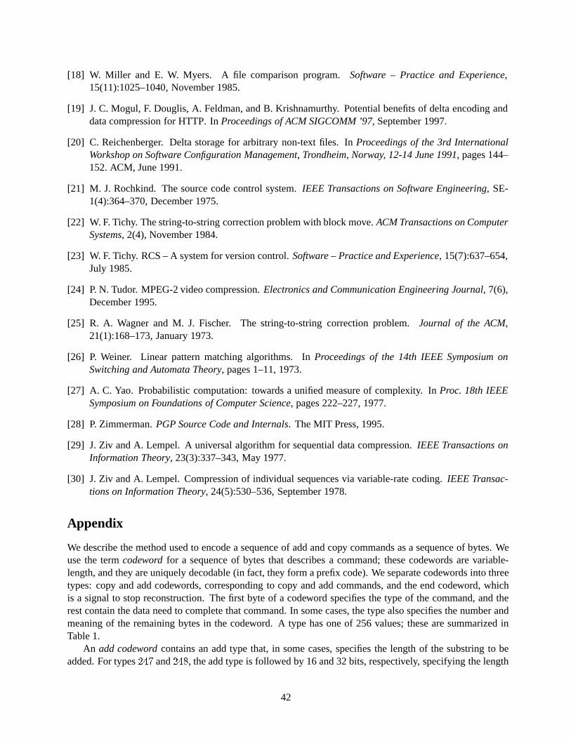
[18] W. Miller and E. W. Myers. A file comparison program. Software – Practice and Experience,15(11):1025–1040, November 1985.

[19] J. C. Mogul, F. Douglis, A. Feldman, and B. Krishnamurthy. Potential benefits of delta encoding anddata compression for HTTP. In Proceedings of ACM SIGCOMM ’97, September 1997.

[20] C. Reichenberger. Delta storage for arbitrary non-text files. In Proceedings of the 3rd InternationalWorkshop on Software Configuration Management, Trondheim, Norway, 12-14 June 1991, pages 144–152. ACM, June 1991.

[21] M. J. Rochkind. The source code control system. IEEE Transactions on Software Engineering, SE-1(4):364–370, December 1975.

[22] W. F. Tichy. The string-to-string correction problem with block move. ACM Transactions on ComputerSystems, 2(4), November 1984.

[23] W. F. Tichy. RCS – A system for version control. Software – Practice and Experience, 15(7):637–654,July 1985.

[24] P. N. Tudor. MPEG-2 video compression. Electronics and Communication Engineering Journal, 7(6),December 1995.

[25] R. A. Wagner and M. J. Fischer. The string-to-string correction problem. Journal of the ACM,21(1):168–173, January 1973.

[26] P. Weiner. Linear pattern matching algorithms. In Proceedings of the 14th IEEE Symposium onSwitching and Automata Theory, pages 1–11, 1973.

[27] A. C. Yao. Probabilistic computation: towards a unified measure of complexity. In Proc. 18th IEEESymposium on Foundations of Computer Science, pages 222–227, 1977.

[28] P. Zimmerman. PGP Source Code and Internals. The MIT Press, 1995.

[29] J. Ziv and A. Lempel. A universal algorithm for sequential data compression. IEEE Transactions onInformation Theory, 23(3):337–343, May 1977.

[30] J. Ziv and A. Lempel. Compression of individual sequences via variable-rate coding. IEEE Transac-tions on Information Theory, 24(5):530–536, September 1978.

Appendix

We describe the method used to encode a sequence of add and copy commands as a sequence of bytes. Weuse the term codeword for a sequence of bytes that describes a command; these codewords are variable-length, and they are uniquely decodable (in fact, they form a prefix code). We separate codewords into threetypes: copy and add codewords, corresponding to copy and add commands, and the end codeword, whichis a signal to stop reconstruction. The first byte of a codeword specifies the type of the command, and therest contain the data need to complete that command. In some cases, the type also specifies the number andmeaning of the remaining bytes in the codeword. A type has one of 256 values; these are summarized inTable 1.

An add codeword contains an add type that, in some cases, specifies the length of the substring to beadded. For types 247 and 248, the add type is followed by 16 and 32 bits, respectively, specifying the length

42

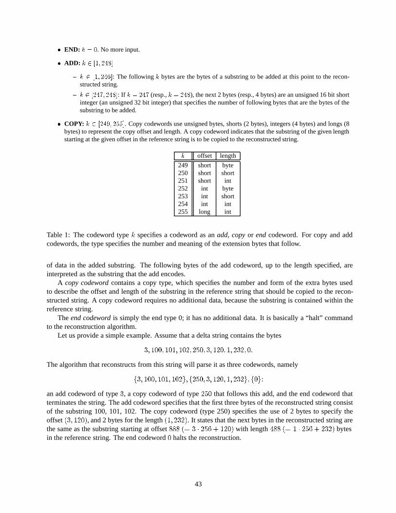
� END: k = 0. No more input.

� ADD: k 2 [1; 248]

– k 2 [1; 246]: The following k bytes are the bytes of a substring to be added at this point to the recon-structed string.

– k 2 [247; 248]: If k = 247 (resp., k = 248), the next 2 bytes (resp., 4 bytes) are an unsigned 16 bit shortinteger (an unsigned 32 bit integer) that specifies the number of following bytes that are the bytes of thesubstring to be added.

� COPY: k 2 [249; 255]. Copy codewords use unsigned bytes, shorts (2 bytes), integers (4 bytes) and longs (8bytes) to represent the copy offset and length. A copy codeword indicates that the substring of the given lengthstarting at the given offset in the reference string is to be copied to the reconstructed string.

k offset length

249 short byte250 short short251 short int252 int byte253 int short254 int int255 long int

Table 1: The codeword type k specifies a codeword as an add, copy or end codeword. For copy and addcodewords, the type specifies the number and meaning of the extension bytes that follow.

of data in the added substring. The following bytes of the add codeword, up to the length specified, areinterpreted as the substring that the add encodes.

A copy codeword contains a copy type, which specifies the number and form of the extra bytes usedto describe the offset and length of the substring in the reference string that should be copied to the recon-structed string. A copy codeword requires no additional data, because the substring is contained within thereference string.

The end codeword is simply the end type 0; it has no additional data. It is basically a “halt” commandto the reconstruction algorithm.

Let us provide a simple example. Assume that a delta string contains the bytes

3; 100; 101; 102; 250; 3; 120; 1; 232; 0.

The algorithm that reconstructs from this string will parse it as three codewords, namely

f3; 100; 101; 102g; f250; 3; 120; 1; 232g; f0g:

an add codeword of type 3, a copy codeword of type 250 that follows this add, and the end codeword thatterminates the string. The add codeword specifies that the first three bytes of the reconstructed string consistof the substring 100, 101, 102. The copy codeword (type 250) specifies the use of 2 bytes to specify theoffset (3; 120), and 2 bytes for the length (1; 232). It states that the next bytes in the reconstructed string arethe same as the substring starting at offset 888 (= 3 � 256 + 120) with length 488 (= 1 � 256 + 232) bytesin the reference string. The end codeword 0 halts the reconstruction.

43