L. Gradilone 1 , S. Artiles 1 , E. Mendoza 1 , I. Morales-Fariña 1

Compact Data Strutures
(To compress is to Conquer)
Antonio Fariña, Javier D. Fernández and Miguel A. Martinez-Prieto
23TH AUGUST 2017
3rd KEYSTONE Training SchoolKeyword search in Big Linked Data

Introduction
Basic compression
Sequences
Bit sequences
Integer sequences
A brief Review about Indexing
PAGE 2
Agenda
images: zurb.com

Compact data structures lie at the intersection of Data Structures (indexing) and Information Theory (compression): One looks at data representations that not only permit space close to the minimum possible (as in compression) but also require that those representations allow one to efficiently carry out some operations on the data.
Introduction to Compact Data Structures
COMPACT DATA STRUCTURES: TO COMPRESS IS TO CONQUERPAGE 3
“
of 784
IntroductionWhy compression?
Disks are cheap !! But they are also slow!
Compression can help more data to fit in main memory.
(access to memory is around 106 times faster than HDD)
CPU speed is increasing faster
We can trade processing time (needed to uncompress data) by space.
of 785
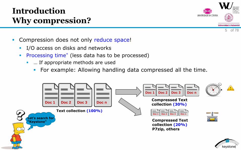
IntroductionWhy compression?
Compression does not only reduce space!
I/O access on disks and networks
Processing time* (less data has to be processed)
… If appropriate methods are used
For example: Allowing handling data compressed all the time.
Text collection (100%)
Doc 1 Doc 2 Doc 3 Doc nCompressed Text collection (30%)
Doc 1 Doc 2 Doc 3 Doc n
Compressed Text collection (20%)P7zip, others
Doc 1 Doc 2 Doc 3 Doc n
Let’s search for “Keystone"
of 786
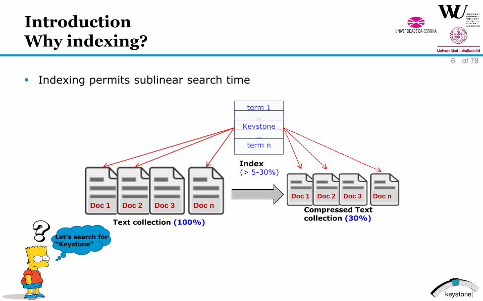
IntroductionWhy indexing?
Indexing permits sublinear search time
Text collection (100%)
Doc 1 Doc 2 Doc 3 Doc nCompressed Text collection (30%)
Doc 1 Doc 2 Doc 3 Doc n
term 1
…
Keystone
…
term n
(> 5-30%)Index
Let’s search for “Keystone"

of 787
IntroductionWhy compact data structures?
Self-indexes:
sublinear search time
Text implicitly kept
Text collection
Doc 1 Doc 2 Doc 3 Doc n
term 1
…
Keystone
…
term n
(> 5-30%)Index
0 0 0 01 1
0 1
0 1 0 10 0
1
0
Self-index (WT, WCSA,…)
term 1
…
Keystone
…
term n
Let’s search for “Keystone"
Introduction
Basic compression
Sequences
Bit sequences
Integer sequences
A brief Review about Indexing
PAGE 8
Agenda
images: zurb.com

Compressing aims at representing data within less space. How does it work? Which are the most traditional compression techniques?
Compression
COMPACT DATA STRUCTURES: TO COMPRESS IS TO CONQUERPAGE 9
“

of 7810
Basic CompressionModeling & Coding
A compressor could use as a source alphabet:
A fixed number of symbols (statistical compressors)
1 char, 1 word
A variable number of symbols (dictionary-based compressors)
1st occ of ‘a’ encoded alone, 2nd occ encoded with next one ‘ax’
Codes are built using symbols of a target alphabet:
Fixed length codes (10 bits, 1 byte, 2 bytes, …)
Variable length codes (1,2,3,4 bits/bytes …)
Classification (fixed-to-variable, variable-to-fixed,…)
-- statisticalInput alphabet
dictionary var2var
Target alphabet
fixed
var
fixed var

of 7811
Basic CompressionMain families of compressors
Taxonomy
Dictionary based (gzip, compress, p7zip… )
Grammar based (BPE, Repair)
Statistical compressors (Huffman, arithmetic, Dense, PPM,… )
Statistical compressors
Gather the frequencies of the source symbols.
Assign shorter codewords to the most frequent symbols.
Obtain compression

of 7812
Basic CompressionDictionary-based compressors
How do they achieve compression?
Assign fixed-length codewords to variable-length symbols (text substrings)
The longer the replaced substring the better compression
Well-known representatives: Lempel-Ziv family
LZ77 (1977): GZIP, PKZIP, ARJ, P7zip
LZ78 (1978)
LZW (1984): Compress, GIF images
of 7813
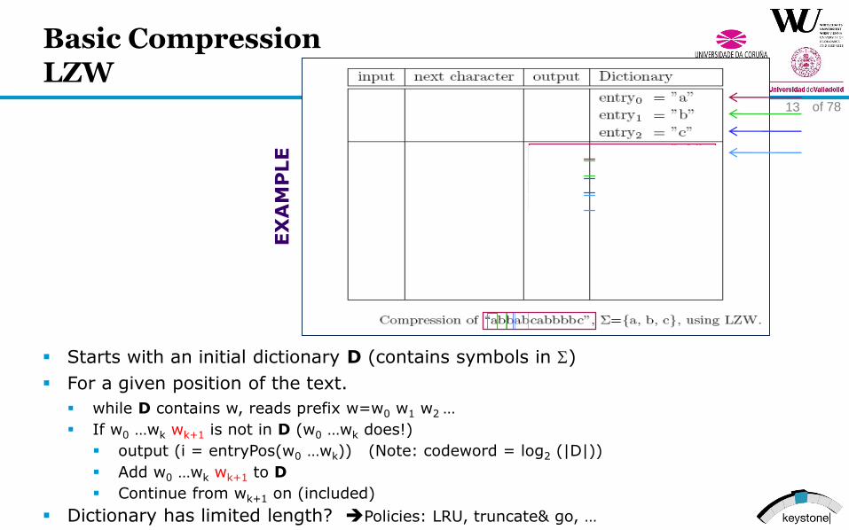
Basic CompressionLZW
Starts with an initial dictionary D (contains symbols in S)
For a given position of the text.
while D contains w, reads prefix w=w0 w1 w2 …
If w0 …wk wk+1 is not in D (w0 …wk does!)
output (i = entryPos(w0 …wk)) (Note: codeword = log2 (|D|))
Add w0 …wk wk+1 to D
Continue from wk+1 on (included)
Dictionary has limited length? Policies: LRU, truncate& go, …
EX
AM
PLE

of 7814
Basic CompressionLZW
Starts with an initial dictionary D (contains symbols in S)
For a given position of the text.
while D contains w, reads prefix w=w0 w1 w2 …
If w0 …wk wk+1 is not in D (w0 …wk does!)
output (i = entryPos(w0 …wk)) (Note: codeword = log2 (|D|))
Add w0 …wk wk+1 to D
Continue from wk+1 on (included)
Dictionary has limited length? Policies: LRU, truncate& go, …
EX
AM
PLE

of 7815
Basic CompressionGrammar-based – BPE - Repair
Replaces pairs of symbols by a new one, until no pair repeats twice
Adds a rule to a Dictionary.
A B C D E A B D E F D E D E F A B E C D
A B C G A B G F G G F A B E C D
H C G H G F G G F H E C D
H C G H I G I H E C D
DE G
AB H
GF I
Source sequence
Dictionary of Rules
Final Repair Sequence

of 7816
Basic CompressionStatistical compressors
Assign shorter codewords to the most frequent symbols
Must gather symbol frequencies for each symbol c in S.
Compression is lower bounded by the (zero-order) empirical entropy of thesequence (S).
Most representative method: Huffman coding
n= num of symbols
nc= occs of symbol c
H0(S) <= log (|S|)n H0(S) = lower bound of the size of S compressed with a zero-order compressor

of 7817
Basic CompressionStatistical compressors: Huffman coding
Optimal prefix free coding
No codeword is a prefix of one another.
Decoding requires no look-ahead!
Asymptotically optimal: |Huffman(S)| <= n(H0(S)+1)
Typically using bit-wise codewords
Yet D-ary Huffman variants exist (D=256 byte-wise)
Builds a Huffman tree to generate codewords

of 7818
Basic CompressionStatistical compressors: Huffman coding
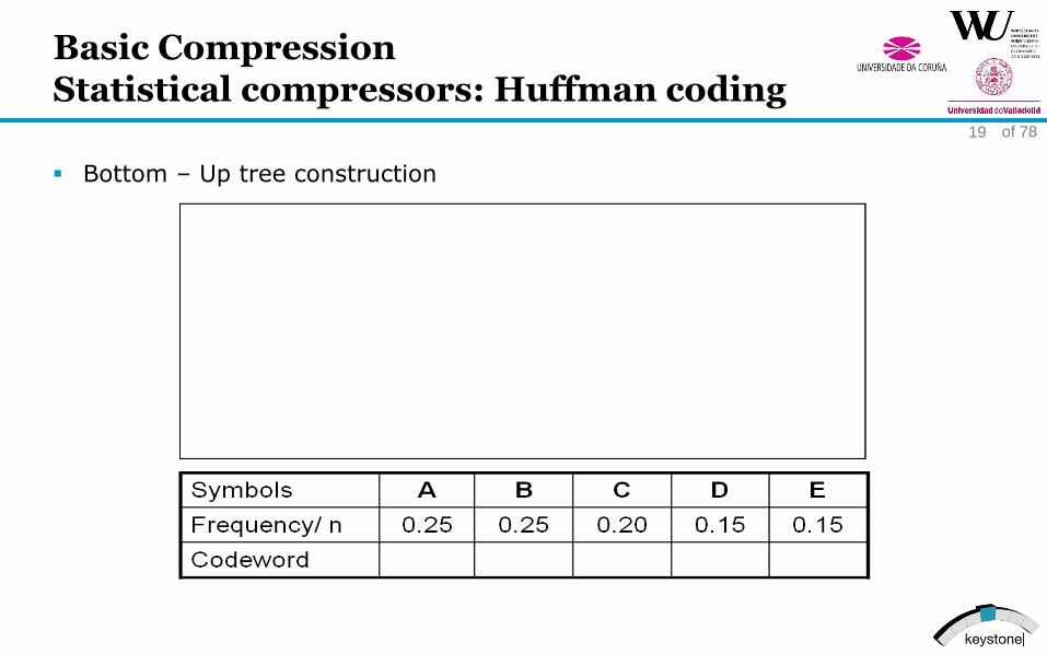
Sort symbols by frequency: S=ADBAAAABBBBCCCCDDEEE
of 7819
Basic CompressionStatistical compressors: Huffman coding
Bottom – Up tree construction

of 7820
Basic CompressionStatistical compressors: Huffman coding
Bottom – Up tree construction

of 7821
Basic CompressionStatistical compressors: Huffman coding
Bottom – Up tree construction

of 7822
Basic CompressionStatistical compressors: Huffman coding
Bottom – Up tree construction

of 7823
Basic CompressionStatistical compressors: Huffman coding
Bottom – Up tree construction

of 7824
Basic CompressionStatistical compressors: Huffman coding
Branch labeling
of 7825
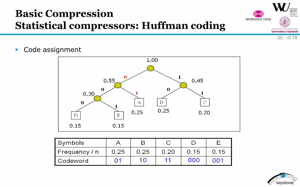
Basic CompressionStatistical compressors: Huffman coding
Code assignment

of 7826
Basic CompressionStatistical compressors: Huffman coding
Compression of sequence S= ADB…
ADB… 01 000 10 …

of 7827
Basic CompressionBurrows-Wheeler Transform (BWT)
Given S= mississipii$, BWT(S) is obtained by: (1) creating a Matrix M with allcircular permutations of S$, (2) sorting the rows of M, and (3) taking the lastcolumn.
mississippi$
$mississippi
i$mississipp
pi$mississip
ppi$mississi
ippi$mississ
sippi$missis
ssippi$missi
issippi$miss
sissippi$mis
ssissippi$mi
ississippi$m
$mississippi
i$mississipp
ippi$mississ
issippi$miss
ississippi$m
mississippi$
pi$mississip
ppi$mississi
sippi$missis
sissippi$mis
ssippi$missi
ssissippi$mi
sort
L = BWT(S)F

of 7828
Basic CompressionBurrows-Wheeler Transform: reversible (BWT-1)
Given L=BWT(S), we can recover S=BWT-1(L)
$mississippi
i$mississipp
ippi$mississ
issippi$miss
ississippi$m
mississippi$
pi$mississip
ppi$mississi
sippi$missis
sissippi$mis
ssippi$missi
ssissippi$mi
LF
1
2
3
4
5
6
7
8
9
10
11
12
Steps:
1. Sort L to obtain F
2. Build LF mapping so that
If L[i]=‘c’, and
k= the number of times ‘c’ occurs in L[1..i], and
j=position in F of the kth occurrence of ‘c’
Then set LF[i]=j
Example: L[7] = ‘p’, it is the 2nd ‘p’ in L LF[7] = 8 which is the 2nd occ of ‘p’ in F
2
7
9
10
6
1
8
3
11
12
4
5
LF

of 7829
Basic CompressionBurrows-Wheeler Transform: reversible (BWT-1)
Given L=BWT(S), we can recover S=BWT-1(L)
$mississippi
i$mississipp
ippi$mississ
issippi$miss
ississippi$m
mississippi$
pi$mississip
ppi$mississi
sippi$missis
sissippi$mis
ssippi$missi
ssissippi$mi
1
2
3
4
5
6
7
8
9
10
11
12
2
7
9
10
6
1
8
3
11
12
4
5
LF
Steps:
1. Sort L to obtain F
2. Build LF mapping so that
If L[i]=‘c’, and
k= the number of times ‘c’ occurs in L[1..i], and
j=position in F of the kth occurrence of ‘c’
Then set LF[i]=j
Example: L[7] = ‘p’, it is the 2nd ‘p’ in L LF[7] = 8 which is the 2nd occ of ‘p’ in F
3. Recover the source sequence S in n steps:
Initially p=l=6 (position of $ in L); i=0; n=12;
In each step: S[n-i] = L[p];
p = LF[p];
i = i+1;
-
-
-
-
-
-
-
-
-
-
-
$
SLF

of 7830
Basic CompressionBurrows-Wheeler Transform: reversible (BWT-1)
Given L=BWT(S), we can recover S=BWT-1(L)
Steps:
1. Sort L to obtain F
2. Build LF mapping so that
If L[i]=‘c’, and
k= the number of times ‘c’ occurs in L[1..i], and
j=position in F of the kth occurrence of ‘c’
Then set LF[i]=j
Example: L[7] = ‘p’, it is the 2nd ‘p’ in L LF[7] = 8 which is the 2nd occ of ‘p’ in F
3. Recover the source sequence S in n steps:
Initially p=l=6 (position of $ in L); i=0; n=12;
Step i=0: S[n-i] = L[p]; S[12]=‘$’
p = LF[p]; p = 1
i = i+1; i=1
$mississippi
i$mississipp
ippi$mississ
issippi$miss
ississippi$m
mississippi$
pi$mississip
ppi$mississi
sippi$missis
sissippi$mis
ssippi$missi
ssissippi$mi
1
2
3
4
5
6
7
8
9
10
11
12
2
7
9
10
6
1
8
3
11
12
4
5
LF
-
-
-
-
-
-
-
-
-
-
-
$
SLF
of 7831
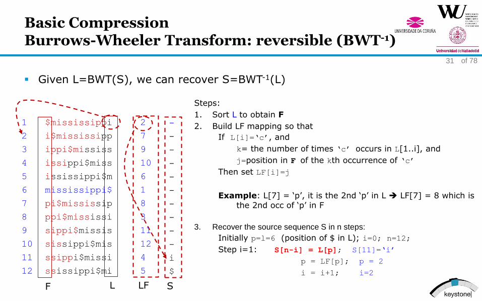
Basic CompressionBurrows-Wheeler Transform: reversible (BWT-1)
Given L=BWT(S), we can recover S=BWT-1(L)
Steps:
1. Sort L to obtain F
2. Build LF mapping so that
If L[i]=‘c’, and
k= the number of times ‘c’ occurs in L[1..i], and
j=position in F of the kth occurrence of ‘c’
Then set LF[i]=j
Example: L[7] = ‘p’, it is the 2nd ‘p’ in L LF[7] = 8 which isthe 2nd occ of ‘p’ in F
3. Recover the source sequence S in n steps:
Initially p=l=6 (position of $ in L); i=0; n=12;
Step i=1: S[n-i] = L[p]; S[11]=‘i’
p = LF[p]; p = 2
i = i+1; i=2
$mississippi
i$mississipp
ippi$mississ
issippi$miss
ississippi$m
mississippi$
pi$mississip
ppi$mississi
sippi$missis
sissippi$mis
ssippi$missi
ssissippi$mi
1
2
3
4
5
6
7
8
9
10
11
12
2
7
9
10
6
1
8
3
11
12
4
5
LF
-
-
-
-
-
-
-
-
-
-
i
$
SLF

of 7832
Basic CompressionBurrows-Wheeler Transform: reversible (BWT-1)
Given L=BWT(S), we can recover S=BWT-1(L)
Steps:
1. Sort L to obtain F
2. Build LF mapping so that
If L[i]=‘c’, and
k= the number of times ‘c’ occurs in L[1..i], and
j=position in F of the kth occurrence of ‘c’
Then set LF[i]=j
Example: L[7] = ‘p’, it is the 2nd ‘p’ in L LF[7] = 8 which isthe 2nd occ of ‘p’ in F
3. Recover the source sequence S in n steps:
Initially p=l=6 (position of $ in L); i=0; n=12;
Step i=1: S[n-i] = L[p]; S[11]=‘i’
p = LF[p]; p = 2
i = i+1; i=2
m
i
s
s
i
s
s
i
p
p
i
$
$mississippi
i$mississipp
ippi$mississ
issippi$miss
ississippi$m
mississippi$
pi$mississip
ppi$mississi
sippi$missis
sissippi$mis
ssippi$missi
ssissippi$mi
1
2
3
4
5
6
7
8
9
10
11
12
2
7
9
10
6
1
8
3
11
12
4
5
LF SLF

of 7833
Basic CompressionBzip2: Burrows-Wheeler Transform (BWT)
BWT. Many similar symbols appear adjacent
MTF.
Output the position of the current symbol within S ‘
Keep the alphabet S ‘= {a,b,c,d,e,… } sorted so that the last used symbol is moved to the begining of S ‘ .
RLE.
If a value (0) appears several times (000000 6 times)
replace it by a pair <value,times> <0,6>
Huffman stage.
Why does it work?In a text it is likely that “he” is preceeded by “t”, “ssisii” by “i”, …
Introduction
Basic compression
Sequences
Bit sequences
Integer sequences
A brief Review about Indexing
PAGE 34
Agenda
images: zurb.com

We want to represent (compactly) a sequence of elements and to efficiently handle them.
(Who is in the 2nd position?? How many Barts up to position 5?? Where is the 3rd Bart??)
Sequences
COMPACT DATA STRUCTURES: TO COMPRESS IS TO CONQUERPAGE 35
“
1 2 3 4 5 6 7 8 9

of 7836
SequencesPlain Representation of Data
Given a Sequence of
n integers
m = maximum value
We can represent it with n ⌈log2(m+1)⌉ bits
16 symbols x 3 bits per symbol = 48 bits array of two 32-bit ints
Direct access (access to an integer + bit operations)
4 1 4 4 4 4 1 4 2 4 1 1 2 3 4 41 2 3 4 5 6 7 8 9 10 11 12 13 14 15 16
100 010 100 100 100 100 001 100 010 100 001 001 010 011 100 1001 2 3 4 5 6 7 8 9 10 11 12 13 14 15 16

of 7837
SequencesCompressed Representation of Data (H0)
Is it compressible?
Ho(S) = 1.59 (bits per symbol)
Huffman: 1.62 bits per symbol
26 bits: No direct access!
(but we could add sampling)
Symbol 4 1 2 3
Occurrences (nc) 9 4 2 1
0 1
16
7
1
43
0
1
2
0
1
2 3 1 4
9
4 1 4 4 4 4 1 4 2 4 1 1 2 3 4 41 2 3 4 5 6 7 8 9 10 11 12 13 14 15 16
1 01 000 0011 1 1 1 01 1 000 1 01 01 1 11 5 10 15 20 25
of 7838
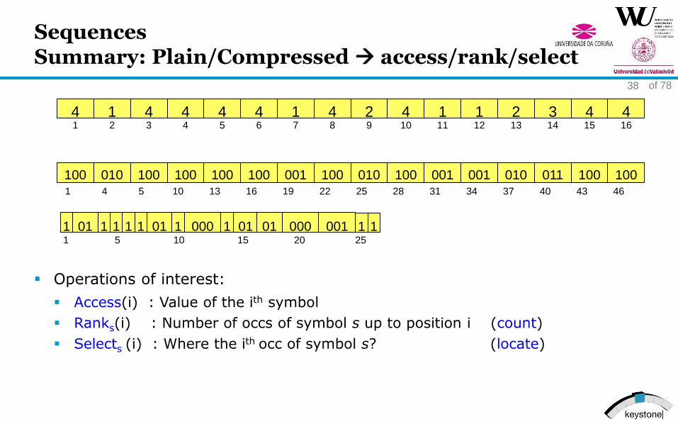
SequencesSummary: Plain/Compressed access/rank/select
Operations of interest:
Access(i) : Value of the ith symbol
Ranks(i) : Number of occs of symbol s up to position i (count)
Selects (i) : Where the ith occ of symbol s? (locate)
4 1 4 4 4 4 1 4 2 4 1 1 2 3 4 41 2 3 4 5 6 7 8 9 10 11 12 13 14 15 16
100 010 100 100 100 100 001 100 010 100 001 001 010 011 100 1001 4 5 10 13 16 19 22 25 28 31 34 37 40 43 46
1 01 000 0011 1 1 1 01 1 000 1 01 01 1 11 5 10 15 20 25
Introduction
Basic compression
Sequences
Bit sequences
Integer sequences
A brief Review about Indexing
PAGE 39
Agenda
images: zurb.com

of 7840
Bit Sequencesaccess/rank/select on bitmaps
Rank1(6) = 3
Rank0(10) = 5
0 1 0 0 1 1 0 1 1 0 0 0 0 0 0 1 0 0 0 0 01 2 3 4 5 6 7 8 9 10 11 12 13 141516 1718 19 20 21
B=
select0(10) =15
access (19) = 0
see [Navarro 2016]

of 7841
Bit SequencesApplications
Bitmaps a basic part of most Compact Data Structures
Example: (We will see it later in the CSA)
S: AAABBCCCCCCCCDDDEEEEEEEEEEFG n log s bits
B: 1001010000000100100000000011 n bits
D: ABCDEFG s log s bits
Saves space:
Fast access/rank/select is of interest !!
Where is the 2nd C?
How many Cs up to position k?
HDT Bitmaps from
Javi's talk !!!
of 7842
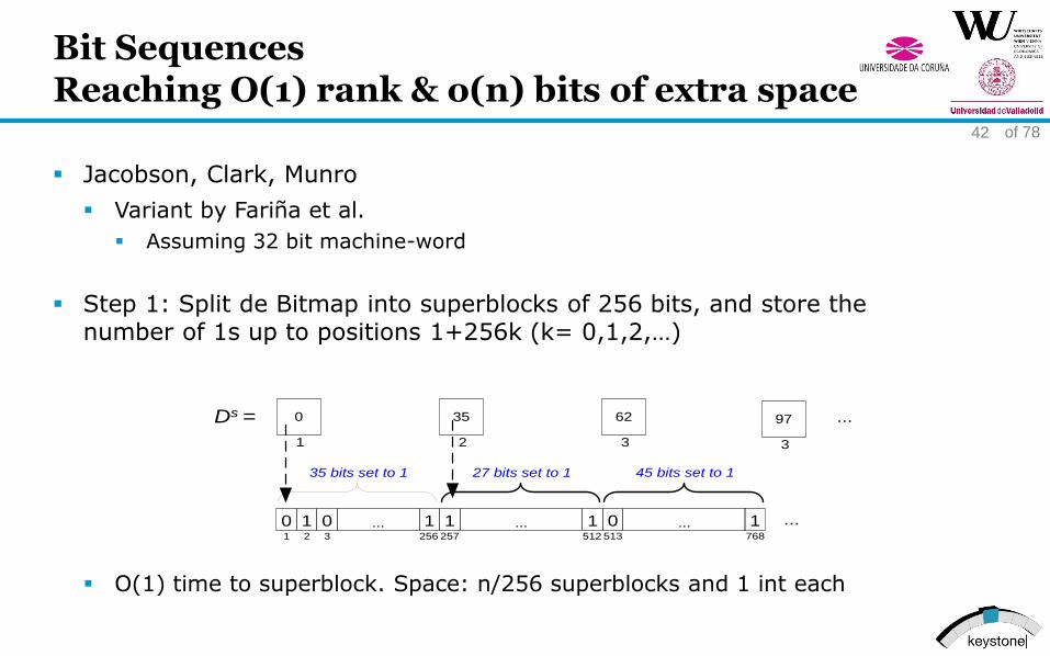
Bit SequencesReaching O(1) rank & o(n) bits of extra space
Jacobson, Clark, Munro
Variant by Fariña et al.
Assuming 32 bit machine-word
Step 1: Split de Bitmap into superblocks of 256 bits, and store thenumber of 1s up to positions 1+256k (k= 0,1,2,…)
O(1) time to superblock. Space: n/256 superblocks and 1 int each
0 1 0 ... 11 2 3 256
35 bits set to 1
1 ... 1257 512
27 bits set to 1
350
1 2
Ds = 62
3
0 ... 1513 768
45 bits set to 1
...
97
3
...

of 7843
Bit SequencesReaching O(1) rank & o(n) bits of extra space
Step 2: For each superblock of 256 bits
Divide it into 8 blocks of 32 bits each (machine word size)
Store the number of ones from the beginning of the superblock
O(1) time to the blocks, 8 blocks per superblock, 1 byte each
1 1 0 ... 11 2 3 256
35 bits set to 1
1 ... 0257 512
27 bits set to 1
350
1 2
Ds = 62
3
0 ... 1513 768
45 bits set to 1
...
97
3
...
1 1 0 ... 11 2 3 32
4 bits set to 1
0 ... 133 64
6 bits set to 1
...
40
1 2
Db = 25
7
...
1 ... 0224 256
8 bits set to 1
300
44

of 7844
Bit SequencesReaching O(1) rank & o(n) bits of extra space
Step 3: Rank within a 32 bit block
Finally solving:
rank1( D , p ) = Ds[ p / 256 ] + Db[ p / 32 ] + rank1(blk, i)
where i= p mod 32
Ex: rank1(D,300) = 35 + 4 + 4 = 43
Yet, how to compute rank1(blk, i) in constant time?
1 0 0 1 0 0 0 0 1 1 0 0 0 1 0 1 1 0 0 0 0 1 0 0 0 1 1 0 0 1 0 1blk =
1 2 3 4 5 6 7 8 9 10 11 12 13 14 15 16 17 18 19 20 21 22 23 24 25 26 27 28 29 30 31 32

of 7845
Bit SequencesReaching O(1) rank & o(n) bits of extra space
How to compute rank1 (blk, i) in constant time?
Option 1: popcount within a machine word
Option 2: Universal Table onesInByte (solution for each byte)
Only 256 entries storing values [0..8]
Finally, sum value onesInByte for the 4 bytes in blk
Overall space: 1.375 n bits
1 0 0 1 0 0 0 0 1 1 0 0 0 1 0 1 1 0 0 0 0 1 0 0 0 1 1 0 0 1 0 1blk =
1 2 3 4 5 6 7 8 9 10 11 12 13 14 15 16 17 18 19 20 21 22 23 24 25 26 27 28 29 30 31 32
0 0 0 0 0 0 0 00 0 0 0 0 0 0 0 0 0 0 0blks =
1 2 3 4 5 6 7 8 9 10 11 12 13 14 15 16 17 18 19 20 21 22 23 24 25 26 27 28 29 30 31 32
1 0 0 1 0 0 0 0 1 1 0 0
Shift 32 – 12 = 20 posicións
Rank1(blk,12)
Val binary OnesInByte
0 00000000 0
1 00000001 1
2 00000010 1
3 00000011 2
252 11111100 6
253 11111101 7
254 11111110 7
255 11111111 8
... ... ...
of 7846
Bit SequencesSelect1 in O(log n) with the same structures
select1(p)
In practice, binary search using rank

of 7848
Bit SequencesCompressed representations
Compressed Bit-Sequence representations exist !!
Compressed [Raman et al, 2002]
For very sparse bitmaps [Okanohara and Sadakane, 2007]
... see [Navarro 2016]
Introduction
Basic compression
Sequences
Bit sequences
Integer sequences
A brief Review about Indexing
PAGE 49
Agenda
images: zurb.com
of 7850
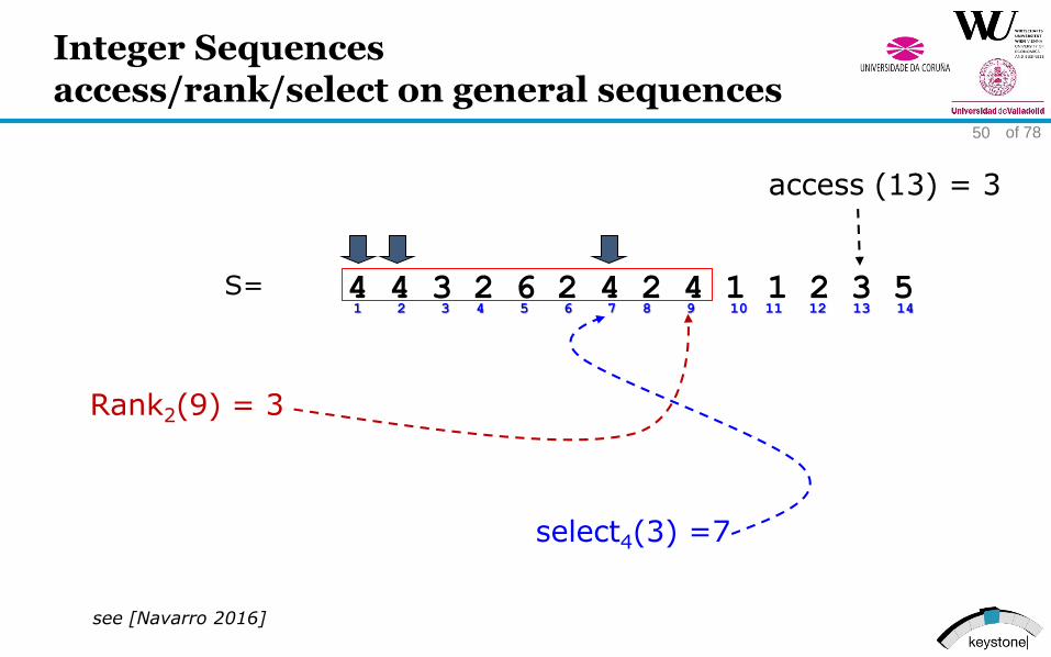
Integer Sequencesaccess/rank/select on general sequences
Rank2(9) = 3
S=
select4(3) =7
access (13) = 3
4 4 3 2 6 2 4 2 4 1 1 2 3 51 2 3 4 5 6 7 8 9 10 11 12 13 14
see [Navarro 2016]
of 7851
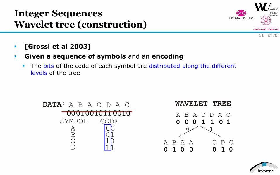
[Grossi et al 2003]
Given a sequence of symbols and an encoding
The bits of the code of each symbol are distributed along the differentlevels of the tree
000100101100 A B A C D A C
0 0 0 0
101 1
0 1
A B A A C D C
0 1 0 10 0
1
0
DATA
SYMBOL CODE
WAVELET TREEA B A C D A C
CD
00011011
BA
Integer SequencesWavelet tree (construction)

of 7852
Searching for the 1st occurrence of ‘D’?
52 OF 74
DATA
SYMBOL CODE
WAVELET TREEA B A C D A C
CD
00011011
BA
A B A C D A C
0 0 0 01 10 1
A B A A C D C
0 1 0 10 0
it is the 2nd bit in B1
Where is the 2nd ‘1’?
at pos 5.
0
1
Where is the1st ‘1’?
at pos 2.
Broot
B0 B1
Integer SequencesWavelet tree (select)

of 7853
Recovering Data: extracting the next symbol
Which symbol appears in the 6th position?
A B A C D A C
0 0 0 01 10 1
A B A A C D C
0 1 0 10 0
Which bit occurs at position 4 in B0?
How many ‘0’s are there up to pos 6?
it is the 4th‘0’
0
1
It is set to 0
The codeword read is ’00’ A
DATA
SYMBOL CODE
WAVELET TREEA B A C D A C
CD
00011011
BA
Broot
B0 B1
Integer SequencesWavelet tree (access)

of 7854
Recovering Data: extracting the next symbol
Which symbol appears in the 7th position?
A B A C D A C
0 0 0 01 10 1
A B A A C D C
0 1 0 10 0
Which bit occurs at position 3 in B1?
How many ‘1’s are there up to pos 7?
it is the 3rd‘1’
0
1
It is set to 0
The codeword read is ’10’ C
TEXT
SYMBOL CODE
WAVELET TREEA B A C D A C
CD
00011011
BA
B1
Broot
B0
Integer SequencesWavelet tree (access)

of 7855
How many C’s are there up to position 7?
A B A C D A C
0 0 0 01 10 1
A B A A C D C
0 1 0 10 0
How many 0s up to position 3 in B1?
How many ‘1’s are there up to pos 7?
it is the 3rd‘1’
0
1
2 !!
TEXT
SYMBOL CODE
WAVELET TREEA B A C D A C
CD
00011011
BA
B1
Broot
B0
Select (locate symbol)
Access and Rank:
Integer SequencesWavelet tree (rank)

of 7856
Each level contains n + o(n) bits
Rank/select/access expected O(log s) time
A B A C D A C
0 0 0 01 10 1
A B A A C D C
0 1 0 10 0
1
0
WAVELET TREE
00010010110010
DATA
SYMBOL CODE
A B A C D A C
CD
00011011
BA
n + o(n) bits
n + o(n) bits
n ⌈log s ⌉ (1 + o(1)) bits
Integer SequencesWavelet tree (space and times)

of 7857
Using Huffman coding (or others) unbalanced
Rank/select/access O(H0(S)) time
A B A C D A C
1 0 1 10 00 1
B C D C A A A
0 1 0 0
0
WAVELET TREE
1 000 1 01 001 1 01
DATA
SYMBOL CODE
A B A C D A C
CD
100001001
BA
nH0(S) + o(n) bits0 1
B D C C
1 0
Integer SequencesHuffman-shaped (or others) Wavelet tree

Introduction
Basic compression
Sequences
Bit sequences
Integer sequences
A brief Review about Indexing
PAGE 58
Agenda
images: zurb.com

Inverted Indexes are the most well-known index for text […]
Suffix Arrays are powerful but huge full-text indexes. Self-indexes trade a more compact space by performance
A brief review about indexing
COMPACT DATA STRUCTURES: TO COMPRESS IS TO CONQUERPAGE 59
“

of 7860
A brief Review about IndexingText indexing: well-known structures from the Web
Traditional indexes (with or without compression)
Inverted Indexes, Suffix Arrays,...
Compressed Self-indexes
Wavelet trees, Compressed Suffix Arrays, FM-index, LZ-index, …
implicit text
auxiliar structure explicit text

of 7861
A brief Review about IndexingInverted indexes
Space-time trade-off
DCCcommunicationscompressionimagedatainformationCliffLogde
0 142
104 165 341506368
219 445
DCC is held at the Cliff Lodge convention center. It is an
international forum for current work on data compression
and related applications. DCC addresses not only
compression methods for specific types of data (text,
image, video, audio, space, graphics, web content, [...]
... also the use of techniques from information theory and
data compression in networking, communications, and
storage applications involving large datasets (including
image and information mining, retrieval, archiving,
backup, communications, and HCI).
99 207 336128 3951925
Vocabulary Posting Lists
Indexed text
Searches
Word posting of that word
Phrase intersection of postingsDo
c1
Do
c2
Compression
- Indexed text (Huffman,...)
- Posting lists (Rice,...)
1
1 22
1 21 21 211
DCCcommunicationscompressionimagedatainformationCliffLodge
Vocabulary Posting Lists
Full-positional information Doc-addressing inverted index
of 7862
A brief Review about IndexingInverted indexes
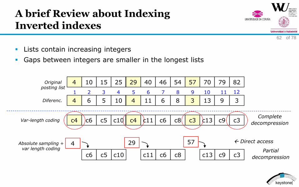
Lists contain increasing integers
Gaps between integers are smaller in the longest lists
4 10 15 25 29 40 46 54 57 70 79 82Original posting list
1 2 3 4 5 6 7 8 9 10 11 12
4 6 5 10 4 11 6 8 3 13 9 3Diferenc.
4
c6 c5 c10
29
c11 c6 c8
57
c13 c9 c3
Absolute sampling + var length coding
Direct access
Partial
decompression
c4 c6 c5 c10 c4 c11 c6 c8 c3 c13 c9 c3Var-length codingComplete
decompression
of 7863
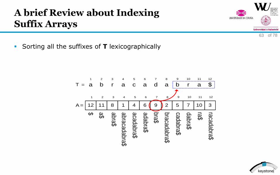
A brief Review about IndexingSuffix Arrays
Sorting all the suffixes of T lexicographically
a b r a c a d a b r a $
1 2 3 4 5 6 7 8 9 10 11 12
T =
12 11 8 1 4 6 9 2 5 7 10 3
1 2 3 4 5 6 7 8 9 10 11 12
A =
abracadabra$
acadabra$
$ a$ adabra$
bra$
bracadabra$
cadabra$
abra$
dabra$
ra$
racadabra$

of 7864
A brief Review about IndexingSuffix Arrays
Binary search for any pattern: “ab”
a b r a c a d a b r a $
1 2 3 4 5 6 7 8 9 10 11 12
T =
12 11 8 1 4 6 9 2 5 7 10 3
1 2 3 4 5 6 7 8 9 10 11 12
A =
P = a b

of 7865
A brief Review about IndexingSuffix Arrays
Binary search for any pattern: “ab”
a b r a c a d a b r a $
1 2 3 4 5 6 7 8 9 10 11 12
T =
12 11 8 1 4 6 9 2 5 7 10 3
1 2 3 4 5 6 7 8 9 10 11 12
A =
P = a b

of 7866
A brief Review about IndexingSuffix Arrays
Binary search for any pattern: “ab”
a b r a c a d a b r a $
1 2 3 4 5 6 7 8 9 10 11 12
T =
12 11 8 1 4 6 9 2 5 7 10 3
1 2 3 4 5 6 7 8 9 10 11 12
A =
P = a b

of 7867
A brief Review about IndexingSuffix Arrays
Binary search for any pattern: “ab”
a b r a c a d a b r a $
1 2 3 4 5 6 7 8 9 10 11 12
T =
12 11 8 1 4 6 9 2 5 7 10 3
1 2 3 4 5 6 7 8 9 10 11 12
A =
P = a b

of 7868
A brief Review about IndexingSuffix Arrays
Binary search for any pattern: “ab”
a b r a c a d a b r a $
1 2 3 4 5 6 7 8 9 10 11 12
T =
12 11 8 1 4 6 9 2 5 7 10 3
1 2 3 4 5 6 7 8 9 10 11 12
A =
P = a b

of 7869
A brief Review about IndexingSuffix Arrays
Binary search for any pattern: “ab”
a b r a c a d a b r a $
1 2 3 4 5 6 7 8 9 10 11 12
T =
12 11 8 1 4 6 9 2 5 7 10 3
1 2 3 4 5 6 7 8 9 10 11 12
A =
P = a b

of 7870
A brief Review about IndexingSuffix Arrays
Binary search for any pattern: “ab”
a b r a c a d a b r a $
1 2 3 4 5 6 7 8 9 10 11 12
T =
12 11 8 1 4 6 9 2 5 7 10 3
1 2 3 4 5 6 7 8 9 10 11 12
A =
locations
Noccs = (4-3)+1Occs = A[3] .. A[4] = {8, 1}
Fast SpaceO(m lg n) O(4n)O(m lg n + noccs) + |T|
P = a b

of 7871
A brief Review about IndexingBWT FM-index
BWT(S) + other structures it is an index
• C[c] : for each char c in S , stores the number of occs
in S of the chars that are lexicographically smaller
than c.C[$]=0 C[i]=1 C[m]=5 C[p]=6 C[s]=8
• OCC(c, k): Number of occs of char c in the prefix of
L: L [1 ..k]
For k in [1..12]
Occ[$] = 0,0,0,0,0,1,1,1,1,1,1,1
Occ[i] = 1,1,1,1,1,1,1,2,2,2,3,4
Occ[m] = 0,0,0,0,1,1,1,1,1,1,1,1
Occ[p] = 0,1,1,1,1,1,2,2,2,2,2,2
Occ[s] = 0,0,1,2,2,2,2,2,3,4,4,4
• Char L[i] occurs in F at position LF(i):
LF(i) = C[L[i]] + Occ(L[i],i)

of 7874
A brief Review about IndexingBWT FM-index
Count (S[1,u], P[1,p])
• Count (S, “issi”)
s
s
i
C[$]=0 C[i]=1 C[m]=5 C[p]=6 C[s]=8
Occ[$] = 0,0,0,0,0,1,1,1,1,1,1,1
Occ[i] = 1,1,1,1,1,1,1,2,2,2,3,4
Occ[m] = 0,0,0,0,1,1,1,1,1,1,1,1
Occ[p] = 0,1,1,1,1,1,2,2,2,2,2,2
Occ[s] = 0,0,1,2,2,2,2,2,3,4,4,4

of 7875
A brief Review about IndexingBWT FM-index
Representing L with a wavelet tree occ is “compressed”

of 7876
Bibliography
1. M. Burrows and D. J. Wheeler. A block-sorting lossless data compression algorithm. Technical Report 124,Digital Systems Research Center, 1994. http://gatekeeper.dec.com/pub/DEC/SRC/researchreports/.
2. F. Claude and G. Navarro. Practical rank/select queries over arbitrary sequences. In Proc. 15th SPIRE,LNCS 5280, pages 176–187, 2008.
3. Paolo Ferragina and Giovanni Manzini. An experimental study of an opportunistic index. In Proc. 12thACM-SIAM Symposium on Discrete Algorithms (SODA), Washington (USA), 2001.
4. Paolo Ferragina and Giovanni Manzini. Indexing compressed text. Journal of the ACM, 52(4):552-581,2005.
5. Philip Gage. A new algorithm for data compression. C Users Journal, 12(2):23–38, February 1994
6. A. Golynski, I. Munro, and S. Rao. Rank/select operations on large alphabets: a tool for text indexing. InProc. 17th SODA, pages 368–373, 2006.
7. R. Grossi, A. Gupta, and J. Vitter. High-order entropy-compressed text indexes. In Proc. 14th SODA,pages 841–850, 2003.

of 7877
Bibliography
8. David A. Huffman. A method for the construction of minimum-redundancy codes. Proc. of the Institute ofRadio Engineers, 40(9):1098-1101, 1952
9. N. J. Larsson and Alistair Moffat. Off-line dictionary-based compression. Proceedings of the IEEE,88(11):1722–1732, 2000
10. U. Manber and G. Myers. Suffix arrays: a new method for on-line string searches. SIAM J. Comp.,22(5):935–948, 1993
11. Alistair Moffat, Andrew Turpin: Compression and Coding Algorithms .Kluwer 2002, ISBN 0-7923-7668-4
12. I. Munro. Tables. In Proc. 16th FSTTCS, LNCS 1180, pages 37–42, 1996.
13. Gonzalo Navarro , Veli Mäkinen, Compressed full-text indexes, ACM Computing Surveys (CSUR), v.39n.1, p.2-es, 2007
14. Gonzalo Navarro. Compact Data Structures -A practical approach. Cambridge University Press, 570pages, 2016
15. D. Okanohara and K. Sadakane. Practical entropy-compressed rank/select dictionary. In Proc. 9thALENEX, 2007.

of 7878
Bibliography
16. R. Raman, V. Raman, and S. Rao. Succinct indexable dictionaries with applications to encoding k-arytrees and multisets. In Proc. 13th SODA, pages 233–242, 2002.
17. Edleno Silva de Moura, Gonzalo Navarro, Nivio Ziviani, and Ricardo Baeza-Yates. Fast and flexible wordsearching on compressed text. ACM Transactions on Information Systems, 18(2):113–139, 2000.
18. Ian H. Witten, Alistair Moffat, and Timothy C. Bell. Managing Gigabytes: Compressing and IndexingDocuments and Images. Morgan Kaufmann, 1999.
19. Ziv, J. and Lempel, A. 1977. A universal algorithm for sequential data compression. IEEE Transactions onInformation Theory 23, 3, 337–343.
20. Ziv, J. and Lempel, A. 1978. Compression of individual sequences via variable-rate coding. IEEETransactions on Information Theory 24, 5, 530–536.

Compact Data Strutures
(To compress is to Conquer)
Antonio Fariña, Javier D. Fernández and Miguel A. Martinez-Prieto
23TH AUGUST 2017
3rd KEYSTONE Training SchoolKeyword search in Big Linked Data
(Thanks: slides partially by: Susana Ladra, E. Rodríguez, & José R. Paramá)