COMP 578 Discovering Clusters in Databases Keith C.C. Chan Department of Computing The Hong Kong...

COMP 578Discovering Clusters in Databases

Keith C.C. Chan

Department of Computing

The Hong Kong Polytechnic University

2

Discovering Clusters

4

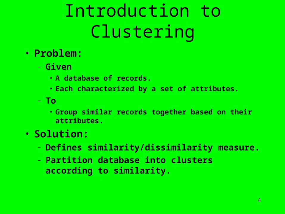
Introduction to Clustering

• Problem:– Given

• A database of records.

• Each characterized by a set of attributes.

– To• Group similar records together based on their attributes.

• Solution:– Defines similarity/dissimilarity measure.– Partition database into clusters according to

similarity.

5

An Example of Clustering:Analysis of Insomnia慢性失眠 68 記憶力下降 5口干 54 目澀 5易醒 53 難集中精神 5難入睡 51 氣促 4疲倦乏力 45 皮膚痕癢 4多夢 37 暗瘡 3頭痛 33 潮熱 3大便干結秘 32 黑眼圈 2痛症 30 鼻塞流涕 2慢性病 28 口渴欲飲 2多尿夜尿 24 抽搐 2上消化道症狀 23 聽力下降 2頭暈 21 聲沙 1心煩 14 煩熱 1心悸 13 震顫 1盜汗 12 視朦 1口苦 12 皮膚干 1急躁或煩躁 9 憂鬱 1胸部不適 8 脫髮 1月經紊亂 8 上瞼下垂 1肢冷 7 口臭 1咳 7 口渴 1易感冒 6 胸部熱 1耳鳴 6 下肢浮腫 1食少 6口或牙痛 6大便溏 5要食西藥 5怕冷 5

FromPatientHistory

6

Analysis of Insomnia (2)•Cluster 1: 多夢易醒型

•多夢 , 易醒 , 難入睡 , 口干 , 大便干結或秘 , 或有頭暈頭痛 , 舌淡紅光滑苔薄白 , 脈弦或滑或弦滑 .

•Cluster 2: 口干易醒難睡型•Cluster 3: 難入睡型•Cluster 4: 多夢難睡型•Cluster 5: 口干型•Cluster 6: 頭痛型

7

Applications of clustering• Psychiatry

– To refine or even redefine current diagnostic categories.

• Medicine– Sub-classification of patients with a particular syndrome.

• Social services – To identify groups with particular requirements or which are

particularly isolated.– So that social services could be economically and effectively

allocated.

• Education – Clustering teachers into distinct styles on the basis of teaching

behaviour.

8

Similarity and Dissimilarity (1)

• Many clustering techniques begin with a similarity matrix.

• Numbers in matrix indicate degree of similarity between two records.

• Similarity between two records ri and rj is some function of their attribute values, i.e. sij = f(ri, rj)

• Where ri = [ai1, ai2, …, aip] and rj = [aj1, aj2, …, ajp] are the attributes values for ri and rj.

9

Similarity and Dissimilarity (2)• Most similarity measures are:

– Symmetric, i.e., sij = sji.– Non negative.– Scaled so as to have an upper limit of unity.

• Dissimilarity measure can be:– dij = 1 - sij– Also symmetric and non negative. – dij + dik djk for all i, j ,k.

– Also called distance measure.

• The most commonly used distance measure is Euclidean distance.

10

Some common dissimilarity measures

• Euclidean distance:

• City block:

• ‘Canberra’ metric:

• Angular separation:

2

1

1

2 ))((

p

kjkik aa

p

kjkik aa

1

||

p

kjkikjkik aaaa

1

)/(||

p

k

p

k jkik

p

k jkik

aa

aa

1 12

122

1

][

11

Examples of a similarity /dissimilarity matrix

000.1475.0350.0005.0750.0

000.1425.0175.0344.0

000.1200.0150.0

000.1062.0

000.1

54321

5

4

3

2

1

S

12

Hierarchical clustering techniques

• Clustering consists of a series of partitions/merging.– May run from a single cluster containing all records

to n clusters each containing a single record.

• Two popular approaches.– agglomerative & divisive methods

• Results may be represented by a dendrogram– Diagram illustrating the fusions or divisions made at

each successive stage of the analysis.

13

Hierarchical-Agglomerative Clustering (1)

• Proceed by a series of successive fusions of n records into groups.

• Produces a series of partitions of the data, Pn, Pn-1, …, P1.

• The first partition Pn, consists of n single-member clusters.

• The last partition P1, consists of a single group containing all n records.

14


• Basic operations:– START:

• Clusters C1, C2, …, Cn each containing a single individual.

– Step 1.• Find nearest pair of distinct clusters, say, Ci and Cj.

• Merge Ci and Cj.

• Delete Cj and decrement number of cluster by one.

– Step 2.• If number of cluster equal one then stop, else return to 1.

15


• Single linkage clustering– Also known as nearest neighbour technique.– The distance between groups is defined as the closest

pair of records from each group.

Cluster BdAB

Cluster A

Single linkage distance

16

Example of single linkage clustering (1)

• Given the following distance matrix.

0.00.30.50.80.9

0.00.40.90.10

0.00.50.6

0.00.2

0.0

54321

5

4

3

2

1

1D

17


• The smallest entry is that for record 1 and 2.• They are joined to form a two-member cluster.• Distances between this cluster and the other

three records are obtained as– d(12)3 = min[d13,d23] = d23 = 5.0– d(12)4 = min[d14,d24] = d24 = 9.0– d(12)5 = min[d15,d25] = d25 = 8.0

18


• A new matrix may now be constructed whose entries are inter-individual distances and cluster-individual values.

0.00.30.50.8

0.00.40.9

0.00.5

0.0

543)12(

5

4

3

)12(

2D

19


• The smallest entry in D2 is that for individuals 4 and 5, so these now form a second two-member cluster, and a new set of distances found– d(12)3 = 5.0 as before– d(12)(45) = min[d14,d15,d25,d25] = d25 = 8.0– d(45)3 = min[d34,d35] = d34 = 4.0

20


• These may be arranged in a matrix D3:

0.00.40.8

0.00.5

0.0

)45(3)12(

)45(

3

)12(D

21


• The smallest entry is now d(45)3 and so individual 3 is added to the cluster containing individuals 4 and 5.

• Finally the groups containing individuals 1, 2 and 3, 4, 5 are combined into a single cluster.

• The partitions produced at each stage are as follows: Stage Groups

P5 [1], [2], [3], [4], [5]P4 [1 2], [3], [4], [5]P3 [1 2], [3], [4 5]P2 [1 2], [3 4 5]P1 [1 2 3 4 5]

22


• Single linkage dendrogram

1

2

3

4

5

0.01.02.03.04.05.0Distance (d)

23

Multiple Linkage Clustering (1)

• Complete linkage clustering– Also known as furthest neighbour technique.– Distance between groups is now defined as that of

the most distant pair of individuals.

• Group-average clustering– Distance between two clusters is defined as the

average of the distances between all pairs of individuals between the two clusters.

24

Multiple Linkage Clustering (2)

• Centroid clustering– Groups once formed are represented by the mean

values computed for each attribute (i.e. a mean vector).

– Inter-group distance is now defined in terms of distance between two such mean vectors.

Cluster BdAB

Cluster A

Complete linkage distance Centroid cluster analysis

dAB

Cluster A

Object B

25

Weaknesses of Agglomerative Hierarchical Clustering

• The problem of Chaining– A tendency to cluster together, at

relatively low level, individuals linked by a series of intermediates.

– May cause the methods to fail to resolve relatively distinct clusters when there are a small number of individuals (noise points) lying between them.

26

Hierarchical - Divisive methods

• Divide n records successively into finer groupings.

• Approach 1: Monothetic– Divide the data on the basis of the possession or otherwise of a

single specified attribute.– Generally used for data consisting binary variables.

• Approach 2: Polythetic– Divisions are based on the values taken by all attributes.

• Less popular than agglomerative hierarchical techniques

27

Problems of hierarchical clustering

• Biased towards finding ‘spherical’ clusters.• Deciding of appropriate number of clusters for

the data is difficult.• Computational time is high due to requirement

to calculate the similarity or dissimilarity of each pair of objects.

28

Optimization clustering techniques (1)

• Form clusters by either minimizing or maximizing some numerical criterion.

• Quality of clustering measured by within-group (W) and between-group dispersion (B).

• W and B can also be interpreted as intra-class and inter-class distance respectively.

• To cluster data, minimize W and maximize B.

• The number of possible clustering partition is vast.

• 2,375,101 possible groupings for just 15 records to be clustered into 3 groups.

29


• To find grouping to optimize clustering criterion, rearranging records and keep new one only if it provides an improvement.

• This is a hill-climbing algorithm known as the k-means algorithm

– a) Generate p initial clusters.– b) Calculate the change in clustering criterion produced by

moving each record from its own to another cluster.– c) Make the change which leads to the greatest improvement

in the value of the clustering criterion.– d) Repeat step (b) and (c) until no move of a single individual

causes the clustering criterion to improve.

30


• Numerical example

Record Variable 1 Variable 2 1 1.0 1.0 2 1.4 2.0 3 3.0 5.0 4 5.0 7.0 5 3.5 6.0 6 4.5 5.0 7 3.5 4.5

31


• Take any two records as initial cluster means, say:

• Remaining records examined in sequence.• They are allocated to the closest group based on

their Euclidean distance to the cluster mean.

Group 1 Group2 Record 1 4

Cluster Mean [1.0, 1.0] [5.0, 7.0]

32


• Compute distance to Cluster Mean leads to the following series of steps.

Group 1 Group 2 Records Distance to

Cluster Mean Records Distance to

Cluster Mean Step 1 1 0 4 0 Step 2 2 1.08 2 6.16 Step 3 3 4.47 3 2.83 Step 4 5 5.59 5 1.80 Step 5 6 5.32 6 2.06 Step 6 7 4.30 7 2.92

•Cluster A={1, 2} Cluster B={3, 4, 5, 6, 7}•Compute new Cluster Means for A and B:

(1.2, 1.5) and (3.9, 5.5)•Repeat until there are no changes in the Cluster Means.

33


Group 1 Group 2 Records Distance to

Cluster Mean Records Distance to

Cluster Mean Step 1 1 0.54 1 5.35 Step 2 2 0.54 2 4.30 Step 3 3 3.94 3 1.03 Step 4 4 6.69 4 1.86 Step 5 5 5.05 5 0.64 Step 6 6 4.81 6 0.78 Step 7 7 3.78 7 1.08

• Second iteration.

•Cluster A={1, 2} Cluster B={3, 4, 5, 6, 7}•Computer new Cluster Means for A and B:

(1.2, 1.5) and (3.9, 5.5)•STOP as there are no changes in the Cluster Means.

34

Properties and problems ofoptimization clustering techniques

• The structure of cluster found is always ‘spherical’.

• Users need to decide how many groups to be clustered.

• The method is scale dependent.• Different solutions may be obtained from the

raw data and from the data standardized in some particular way.

35

Clustering discrete-valued data (1)

– Basic concept• Based on a simple voting principle called Condorset.

• Measure distance between input records and assign them to specific clusters.

• Pairs of records are compared by the values of the individual fields.

• No. of fields with same values determine the degree to which the records are similar.

• No. of fields with different values determine the degree to which the records are different.

36

Clustering discrete-valued data - (2)

• Scoring mechanism– When a pair of records has the same value for the

same field, the field gets a vote of +1.– When a pair of records does not have the same value

for a field, the field gets a vote of -1.– The overall score is calculated as the sum of scores

for and against placing the record in a given cluster.

37


• Assignment of record to a cluster– A record is assigned to a cluster if the overall score

of that cluster is the highest among all other clusters.

– A record is assigned to a new cluster if the overall scores of all clusters turn out to be negative.

38


• There are a number of passes over the set with records, and therefore the cluster centers are reviewed for potential reassignment to a different cluster.

• Termination criteria– Maximum number of passes is achieved.– Maximum number of clusters is reached.– Cluster centers do not change significantly as

measured by a user-determined margin.

39

An Example - (1)

• Assume 5 records with 5 fields, each field takes on a value either 0, 1 or 2:– record 1 : 0 1 0 2 1 – record 2 : 0 2 1 2 1– record 3 : 1 2 2 1 1– record 4 : 1 1 2 1 2– record 5 : 1 1 2 0 1

40

An Example - (2)

• Creation of first cluster:– Since record 1 is the first record of the data set, it is

assigned to cluster 1.

• Addition of record 2:– Comparison between record 1 and 2:

• Number of positive vote = 3

• Number of negative vote = 2

• Overall score = 3-2 = 1

• Since the overall score is positive, record 2 are assigned to cluster 1.

41

An Example - (3)

• Addition of record 3:– Score between record 1 and 3 = -3– Score between record 2 and 3 = -1– Overall score for cluster 1 = score between record

1,3 and 2,3 = -3 + -1 = -4– Since the overall score is negative, record 3 is

assigned to a new cluster (cluster 2).

42

An Example - (4)

• Addition of record 4:– Score between record 1 and 4 = -3– Score between record 2 and 4 = -5– Score between record 3 and 4 = 1– Overall score for cluster 1 = -8– Overall score for cluster 2 = 1– Therefore, record 4 is assigned to cluster 2.

43

An Example - (5)

• Addition of record 5:– Score between record 1 and 5 = -1– Score between record 2 and 5 = -3– Score between record 3 and 5 = 1– Score between record 4 and 5 = 1– Overall score for cluster 1 = -4– Overall score for cluster 2 = 2– Therefore, record 5 is assigned to cluster 2.

44

An Example - (6)

• Overall cluster distribution of 5 records after iteration 1:– Cluster 1 : record 1 and 2– Cluster 2 : record 3, 4 and 5

COMP 578 Discovering Clusters in Databases Keith C.C. Chan Department of Computing The Hong Kong...

Documents

Transcript of COMP 578 Discovering Clusters in Databases Keith C.C. Chan Department of Computing The Hong Kong...