Admission Control in Cellular

Communications Networks

by

Dimitri A. Papaioannou

Submitted to the

Department of Electrical Engineering and Computer Science

in partial fulfillment of the requirements

for the degree of

Master of Science

at the

MASSACHUSETTS INSTITUTE OF TECHNOLOGY

June 1997

@ Massachusetts Institute of Technology,All rights reserved.

M 7Author ..

--- " -epartment of Electrical Engineering and Computer ScienceJune 18, 1997

Certified by...Dimitri P. Bertsekas

Ie) s ofeps oLZf Electrical Engineering-;7

Accepted by .....

-esis Supervisor

Arthur C. ..Smith.Arthur C. Smith

Chairman, Department Committee on Graduate Students

Channel Allocation and

Channel Allocation and Admission Control in Cellular

Communications Networks

by

Dimitri A. Papaioannou

Submitted to the Department of Electrical Engineering and Computer Scienceon June 18, 1997, in partial fulfillment of the

requirements for the degree ofMaster of Science

Abstract

In Frequency Divided Multiple Access cellular communication systems a limited frequencyis divided into orthogonal channels that are assigned to mobile subscribers. Channels thatare in use in a certain cell site cannot be reused in neighboring cells due to co-channel in-terference. One of the challenges in providing multimedia wireless services is to maximizethe service provided and maintain certain quality measures subject to the restrictions ofbandwidth and channel reuse constraints by implementing good call admission and channelassignment strategies. In this thesis, the problem of call admission and channel allocation ina cellular network is formulated as a continuous time controlled Markov process and approx-imate dynamic programming is used, with conjunction with compact state representationarchitectures to obtain call admission and channel allocation policies.

Thesis Supervisor: Dimitri P. BertsekasTitle: Professor of Electrical Engineering

Acknowledgments

I would like to thank professor Dimitri Bertsekas for his help and guidance in this research

and for the inspiration he provided with his enthusiasm for the subject.

I would also like to thank my office mates who have made my stay at LIDS comfortable

and enjoyable. I am grateful for their help and their support and most importantly for their

friendship. I would also like to thank the members of the NDP group who have guided me

with their advice, inspired me with their dedication and team spirit, and shared with me

many happy occasions.

I would like to thank my dear friends Marina, Apostolos, Vaggelis, Panagiotis, and Aris who

are far in distance but always close to my heart. I would like to thank John, Karin, and

Angela for being my family away from home, and Silvia for her constant support.

Finally, I would like to thank my parents Alexandros and Despina and my sister Natalia who

have been a source of love and inspiration throughout my life. I owe my every accomplishment

to them, including the completion of this thesis.

Contents

1 Introduction

1.1 Problem Statem ent . . . . . . . . . . . . . . . . . . . . . . . . . . . . . . . .

1.2 NDP M ethodology . . . . . . . . . . . . . . . . . . . . . . . . . . . . . . ..

1.2.1 The Dynamic Programming Methodology and its Limitations . . . . .

1.2.2 Formulation of the Dynamic Programming Problem, and the Policy

Iteration Algorithm ..... ........... ........... .

1.2.3 Compact Representation Methods and Approximate Policy Iteration .

1.3 Thesis Presentation ..........................

2 Pro

2.1

2.2

2.3

2.4

blem Description

Description of a Cellular System . . .

Operation of a Cellular System . . .

Performance Measures ........

Channel Allocation Schemes .....

2.4.1 Fixed Channel Allocation ..

2.4.2 Dynamic Channel Allocation

2.4.3 Hybrid Channel Allocation .

2.4.4 Handoff Prioritizing Schemes.

17

.. ... ... .... ... .... ... 17

. .... ... .... ... .... ... 18

. .... ... .... ... .... .. . 19

. .... ... .... .. ..... .. . 19

. .... ... .... .. ..... .. . 19

. .... ... .... .. .... ... . 19

. .... ... ... ... ... .... . 20

. .... ... ... ... ... .... . 2 0

3 Continuous Time Controlled Markov Processes and Dynamic Program-

ming

3.1 Continuous Time Controlled Markov Processes .................

3.2 Uncontrollable State Components ........................

4 Problem Formulation

4.1 Formulation of the Problem as a Markov Decision Process ..........

4.2 Motivation and Implementation .........................

4.3 The Channel Allocation Problem without Handoffs . ..............

4.3.1 Description of Training Parameters and Experimental Results . .

4.4 The Call Admission Problem with Handoffs

4.4.1 Small Systems: Exact Results and Simulation . ............

4.4.2 Large Systems: Comparison of Features and Methodologies ......

4.5 Conclusions of this Section ............................

5 Conclusion

5.1 Discussion of Results ..........

5.2 Extensions and Possible Improvements

5.2.1 Extensions ............

5.2.2 Possible Improvements . . . . .

22

22

26

.. ..... . 58

60

.. ... .... .... .... 60

. . . . . . . . . . . . . . . . . . 60

List of Figures

4-1 Comparison of heuristic policies and approximate dynamic programming with

optimistic TD(0) for a system with uniform traffic. . ............... 32

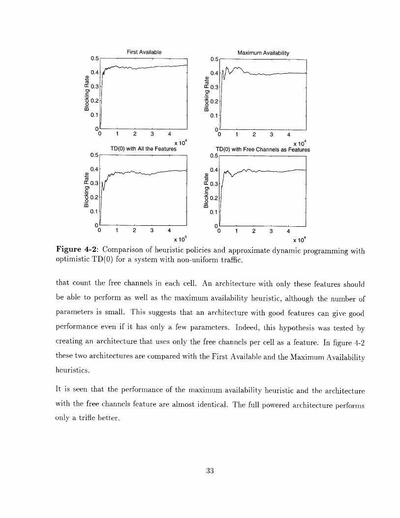
4-2 Comparison of heuristic policies and approximate dynamic programming with

optimistic TD(0) for a system with non-uniform traffic. . ............ 33

4-3 Illustration of the optimal cost-to-go and optimal policy for a 2-cell system

with 10 channels. It is always optimal to accept in cell 1, while the acceptance

in cell 2 is a generalized threshold policy. . .................. . 38

4-4 Illustration of the optimal cost-to-go and optimal policy for a 2-cell system

with 10 channels. ................................. 40

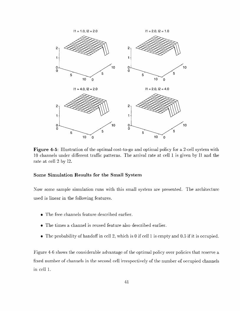
4-5 Illustration of the optimal cost-to-go and optimal policy for a 2-cell system

with 10 channels under different traffic patterns. The arrival rate at cell 1 is

given by 11 and the rate at cell 2 by 12. ..................... 41

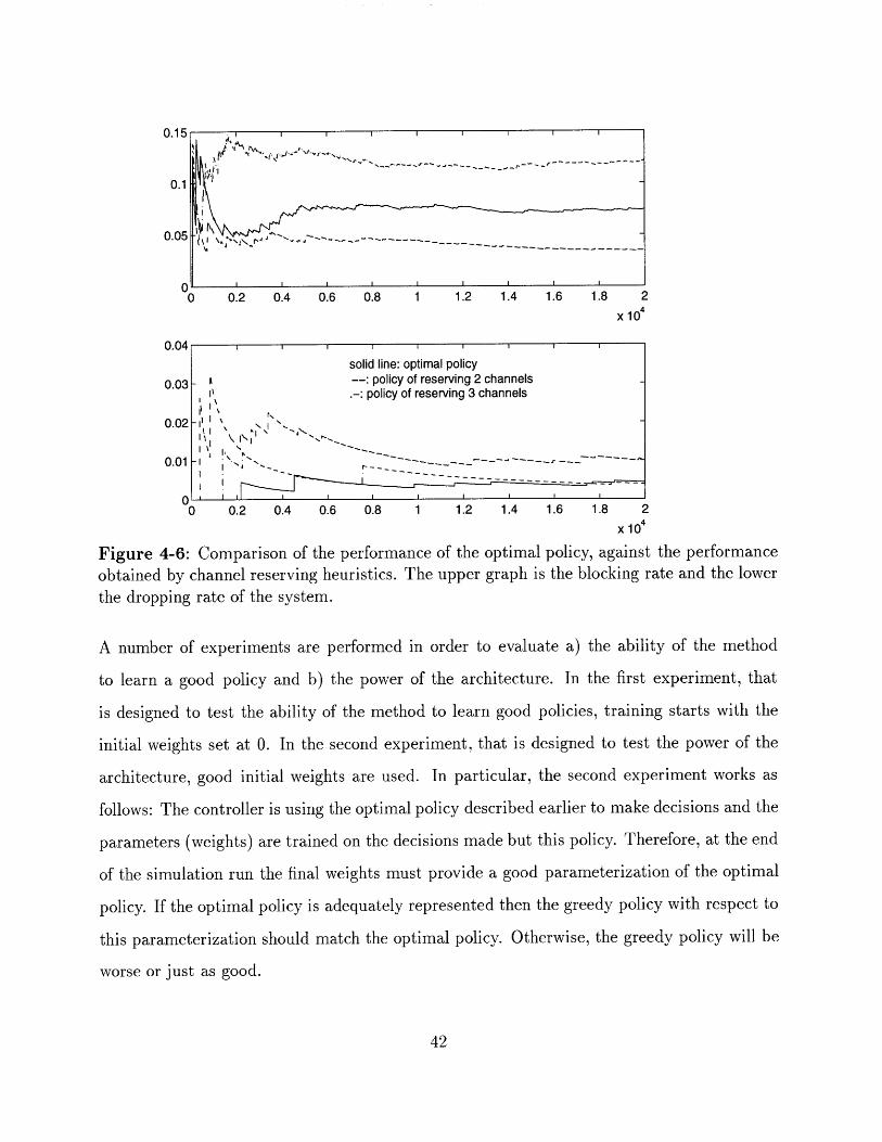
4-6 Comparison of the performance of the optimal policy, against the performance

obtained by channel reserving heuristics. The upper graph is the blocking rate

and the lower the dropping rate of the system. . ................. 42

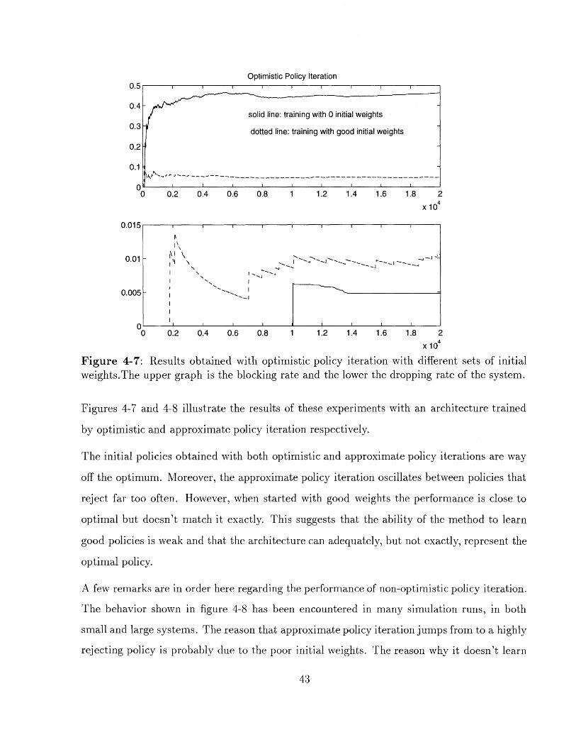
4-7 Results obtained with optimistic policy iteration with different sets of initial

weights.The upper graph is the blocking rate and the lower the dropping rate

of the system. ............ .. ... ................. .... 43

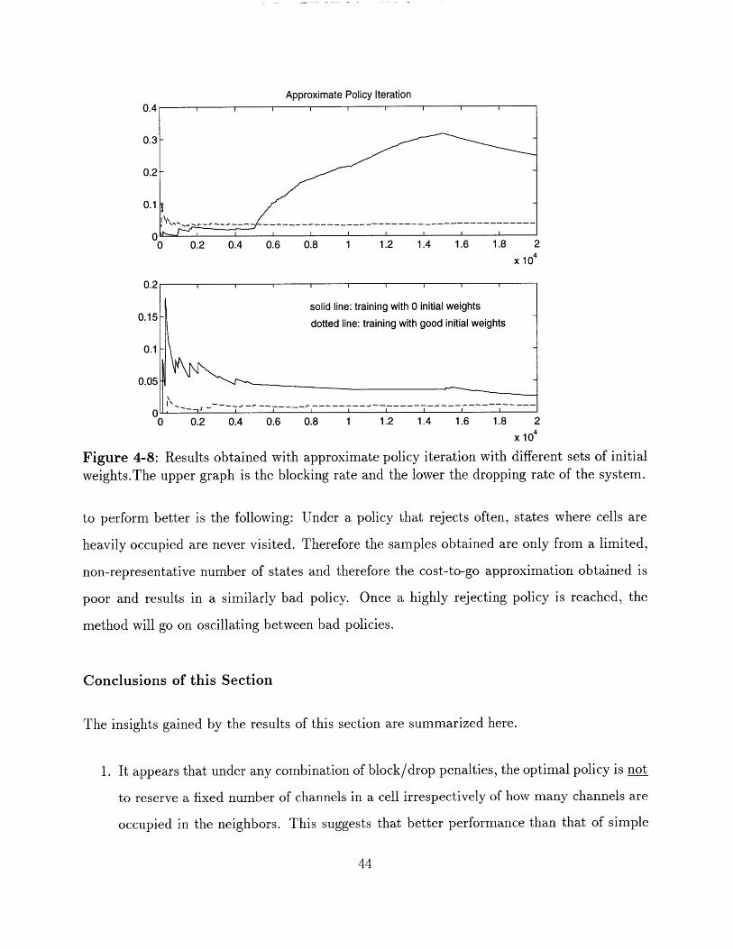
4-8 Results obtained with approximate policy iteration with different sets of initial

weights.The upper graph is the blocking rate and the lower the dropping rate

of the system. .................. ................. 44

4-9 Performance of heuristic policies. ............... . . . . . . . . .... 48

4-10 Performance of certain architectures trained by TD(0) in a system with uni-

form handoff probability .............................. 49

4-11 Performance of certain architectures trained by TD(0) in a system with uni-

form handoff probability .............................. 50

4-12 Performance of TD(0) in a system with uniform handoff probability and good

initial weighs for a system with uniform handoff probability. . .... .. .. 51

4-13 Performance of TD(0) in a system with uniform handoff probability and good

initial weighs for a system with uniform handoff probability . ...... . 52

4-14 Performance of heuristic policies in a system with non-uniform handoff prob-

abilities. . . . . . . . . . . . . . . . . . . . . . . . . . . . . . . . . . . . . .. . 53

4-15 Performance of TD(0) in a system with non-uniform handoff probability. . 54

4-16 Performance of TD(0) in a system with non-uniform handoff probability. . 55

4-17 Performance of TD(0) in a system with non-uniform handoff probability and

good initial weights. . .. .. . . . . . .. .. ... .. . . . . . .. .... 56

4-18 Performance of TD(0) in a system with non-uniform handoff probability and

good initial weights.................................

Chapter 1

Introduction

1.1 Problem Statement

In Frequency Divided Multiple Access cellular communication systems a limited frequency is

divided into orthogonal channels that are assigned to mobile subscribers. Channels that are in

use in a certain cell site cannot be reused in neighboring cells due to co-channel interference.

One of the challenges in providing multimedia wireless services is to maximize the service

provided and maintain certain quality measures subject to the restrictions of bandwidth and

channel reuse constraints.

The quality of service is typically measured by the probability with which a user is denied

service and the probability with which a call is terminated before completion. The first

performance measure is called new call blocking probability and the second handoff blocking

probability or call dropping. New call blocking occurs when a user attempting a call is denied

access to the network, typically because there is no available channel. Handoff blocking

occurs when an ongoing call is forced to terminate before completion. This occurs when the

mobile subscriber crosses cell boundaries and there is no available channel in the new cell.

Handoff blocking is highly undesirable and in many cellular systems a number of channels,

called guard channels is reserved for handling only handoff calls. A significant challenge is to

design a channel allocation and call admission strategy to minimize handoff blocking while

maintaining the new call blocking probability at an admissible level.

In this thesis the call admission and channel assignment problem is formulated as a continuous

time Markov decision problem. The number of states is finite but huge, thus the optimal

solution is computationally intractable. In order to obtain good suboptimal policies, the cost

function of the problem is approximated by a parameterized architecture. The architecture is

trained by approximately policy iteration via simulation to obtain values for the parameters

that will describe good policies.

1.2 NDP Methodology

1.2.1 The Dynamic Programming Methodology and its Limitations

The theory of dynamic programming provides a unifying mathematical framework for sequen-

tial decision-making under uncertainty. Most dynamic decision problems can be cast into a

dynamic program formulation. Ideally, one would like to use the theory of dynamic program-

ming to obtain closed-form analytical expressions of an optimal policy. However, because of

the nonlinear character of the dynamic programming equations, an analytical solution is often

not possible. Although there are iterative numerical algorithms that, in principle, converge

to the optimal policy, these algorithms cannot be applied to very complex problems, because

the computational burden becomes excessive. This barrier on the successful application of

dynamic programming to practical problems was termed by Bellman the "curse of dimen-

sionality", referring mainly to the severe computational requirements when attempting to

tackle large-scale, dynamic decision problems. Furthermore, the dynamic programming for-

mulation depends on an accurate mathematical model of the underlying dynamic system and

the decision-maker's objectives. However, in many complex problems of practical interest,such a model is not available.

The idea behind approximate dynamic programming is to develop a methodology which allows

the practical application of dynamic programming to problems that suffer either from the

curse of dimensionality or by the lack of an accurate mathematical model. This methodology

combines the theory of dynamic programming, function approximation techniques, and the

use of computer simulation to provide the basis for a rational approach to complex, sequential

decision problems under uncertainty.

1.2.2 Formulation of the Dynamic Programming Problem, and the

Policy Iteration Algorithm

Consider a discrete-time dynamic system evolving under the equation

Xk+l = f(xk, Uk, Wk) (1.1)

where xk, represents the state, wk a random disturbance, and uk a control action chosen from

some appropriate set of controls U(xk).

In the infinite horizon, discounted version of the dynamic programming formulation the ob-

jective is to choose the control actions Xk in such a way as to minimize the expected value of

an additive discounted cost

J*(xo) = E ak k, g k, Wk) (1.2)k=0

where a E (0, 1) is a discount factor, and g(x, u, w) is the one-stage cost function.

A stationary policy u is a function mapping states to controls and the cost-to-go of p starting

at state xo is defined to be

J,(xo) = E akg(Xk, P (k), k)k=0

(1.3)

It can be shown [1] that if the one-stage costs are bounded then then J*(x) and J,(x) are the

unique solutions of the Bellman equations

and

J*(x) min E {g(x, u, w,) + aJ(f(x, u, w)}uEU(x)

J,(x) = E {g(x, y(x), w,) + aJ(f(x, fu(x), w)}

(1.4)

(1.5)

where the expectation is taken with respect to the random parameter w.

When the state space and disturbance spaces are finite, it can be shown that the right hand

sides of equations (1.4) and (1.5) respectively can be written as

and

(TJ)(i) mim g(i, u) + a pi,(u) J(j)uEU(i) j

n

(TJg)(i) g(i, p(i)) + a~ p(a(i))J(j)j=1

(1.6)

(1.7)

where the states are now represented by integers i and pij denotes the transition probabilities

from state i to state j. Also the dynamic programming operators T and T, are defined for

convenience.

In this case the following algorithm, known as policy iteration can be used to obtain the

optimal cost-to-go for the dynamic program.

The algorithm starts with an arbitrary initial policy 'o and then performs the following two

steps

Step 1: Given the policy yk, perform a policy evaluation step that computes the solution to

the linear system of equations Jk(i) = Tk J(i), i= 1,... ,n.

Step 2: We then perform a policy improvement step which computes a new policy pk+1 as

pk+1(i) = arg min [ g(i,u)+Pij(u) Jk(] = 1 . ,n.uEU(i)

If Jk+1 (i) = Jk(i) for all i, then the algorithm terminates with policy pk. Otherwise, we

repeat Steps 1-2 replacing pk with the new policy 1 k+y1

1.2.3 Compact Representation Methods and Approximate Policy

Iteration

Let J*(i) denote the optimal expected cost from state i. The neuro-dynamic programming

methodology attempts to approximate this function by a class of functions J(i, r), para-

meterized by a vector r, termed a compact representation or an architecture. If the class of

functions described by the parameterization is wide enough then, by adjusting the parameters

r through training, a good approximation to the optimal objective function may be obtained.

The measure of closeness to the optimal cost-to-go is measured by the sup norm

V|J - J*| = sup IJ(i)- J*(i)

and is referred as the power of the architecture. Unfortunately, in most cases, the power of the

architecture cannot be known beforehand. The parameters of the architecture are updated

by the following algorithm known as Approximate Policy Iteration.

Approximate Policy Iteration

Approximate Policy Iteration, like normal policy iteration, consists of two stages: policy

evaluation and policy improvement. The policy evaluation step is performed approximately

via Monte-Carlo simulation and the policy improvement step is obtained by training the

weight vector r. The procedure works as follows:

Given a policy y, the cost-to-go J, associated with this policy is not known. Instead, we have

an approximation architecture provided by the function J(i, r,) evaluated at a specific set of

parameters or weights r,. The Approximate Policy Iteration algorithm works as described

below:

First, an initial set of parameters ro is chosen, possibly parameterizing some known initial

policy. Then the following steps are performed.

policy improvement An initial state io is chosen, where by trajectories are generated as

follows: From each state i, an action is chosen from the set of available actions U(i) by

computing

/-k+ (i) = arg min g(i, u) + pi, (u)(j, r,k))

Then the next state is selected according to the probabilities pij(ltk+l(i)), and following

the state transition from i to j, the cost g(i,pk+l(i)) is incurred. Let the number of

steps starting from a state i until trajectory termination be denoted by M(i) (M(i)

may be deterministic or a random variable). For each state i that is visited during the

trajectory, a cost sample c(i, m) is computed, where m denotes the mth simulation run.

policy evaluation When a satisfactory number of cost samples is obtained for each state

visited, the new policy is evaluated by a policy evaluation step, which amounts to

computing appropriate values for the parameter vector r,k+1

Let S denote the set of states that has been visited, and M(i) the number of cost

samples that have been obtained for each state i. A way of obtaining the set of weights

corresponding to this new policy is by solving the Least Squares problem

M(i)

min (J(i, r) - c(i, ))(1.8)

iES m=1

Approximate Policy Iteration with TD(A)

The linear least squares problem (1.8) can be solved iteratively by the following method.

After simulating the mth trajectory io,... iN, update the weights by the relation

N-1

rm+1 = rm - ym VJ(ik,

k=O

r) J(ik, r)

N-1

- E g(imY (im) im+i))m=k

where 7m is a suitably chosen step-size.

By defining dk = (ik, ik+l)+ J(ik+l, r) - J(ik, r), the incremental algorithm (1.9) can be

written as

N-1

rm+, = rm - "^m E VJ(ik, r)(dk + dk+l +... + dN-1)

k=O

(1.10)

The dks are called temporal differences. There is a variant of this iterative algorithm that is

motivated by learning methods and is known as TD(A) . In TD(A) the temporal differences

obtained at earlier stages are discounted by a factor of A E [0, 1].

N-1 N-1

rm+1 = rm -m S VJ(ik, r) dk k-m

k=O k=m

(1.11)

The iterative algorithm 1.11 can be used in two different scenaria.

(1.9)

1. The parameters r, are stored in a place in memory different from the place where r is

stored and the updates are performed after a satisfactory number of trajectory runs.

2. The parameters are updated after each trajectory run. In this case, instead of J(ik, r),

J(ik, rm) appears on the right side of (1.10). It is also possible to update the weights

after each state transition. This method, called Optimistic Policy Iteration, is actually

not a true policy iteration because the parameters are updated before there is enough

statistical data to evaluate the present policy. Although it is not clear whether this

algorithm will produce improved policies and there is no theory to support such an

assumption, it has been successful in many practical cases [21].

Feature-Based Architectures

It was mentioned earlier that finding an appropriate parameterized class of functions J(i, r)

is essential for the performance of these methods. A popular choice of architecture is based

on Neural Networks that have been theoretically shown to be universal approximators for any

continuous function defined in some bounded interval [11]. Furthermore, they have known

considerable experimental success. The drawback of using Neural Networks on a problem

of large dimension is that they get increasingly harder to train as the number of parameters

increases.

Another approach is to simplify the state before it becomes an input to the architecture byforming a reduced state representation. A way to construct a reduced representation of the

state is through the use of features. Features are important characteristics of the state that

describe numerically intuitive facts or heuristic policies for the system under question, and

aim to capture the prevailing characteristics of the problem. For example, in a game of poker,important features of the state (a hand of cards in this case) would be the number of cards

of equal value in the hand, the highest card, the number of cards of the same suit, etc...

Given k features, f1i,... , fk, a reduced state architecture can be defined by making it a

function of the features and the weights J(f(i), r). If the features are good, in the sense

that they capture the essential nonlinearities of the problem, then the functional form of the

architecture need not be very complicated. Indeed, for many problems, a linear feature-based

architecture J(f(i), r) = fk(i)rk can give very good results [19], [2].

1.3 Thesis Presentation

This thesis is organized as follows. In chapter 2, the nature of the channel allocation and call

admission problem in cellular networks is described and a review of related work in the field

is presented.

In chapter 3, the dynamic programming approach for solving continuous time Semi-Markov

decision problems is described.

In chapter 4 the channel allocation and call admission problem is formulated in the sequential

Markov decision framework. Details of the simulation are discussed and experimental results

presented.

In chapter 5 the conclusions and suggestions for future work are discussed.

Chapter 2

Problem Description

2.1 Description of a Cellular System

This thesis attempts to solve the problem of admission control and channel allocation in

a cellular communications network. In this chapter the operation of a cellular network is

described and related work in the field is described.

A cellular communications system consists of the following units.

ing Office (MTSO), which is the central coordinating element.

cessor and cellular switch and is responsible for controlling the

billing activities.

A Mobile Telephone Switch-

It contains the cellular pro-

call processes and handling

The mobile units, which are mobile telephones containing a control unit, a transceiver, and

an antenna.

The base stations or cell cites which is a fixed interconnected network providing the interface

between the mobiles and the MTSO. Each cell site has a control unit, radio cabinets, antennas,a power plant, and data terminals. The base station communicates with the MTSO and the

mobile units via wireless data links.

The geographical area within which a mobile unit can communicate with a particular base

station is called a cell. Cells have approximately circular shape and are overlapping to

ensure the continuity of communications when users are migrating form one cell to another.

However, cells are usually depicted as non-overlapping hexagonal regions to facilitate analysis

and simulation.

2.2 Operation of a Cellular System

A set of fixed set of frequency ranges called channels is allocated to each base station. When

a mobile unit wants to communicate with another mobile or the base station it sends a call

request to the base station with the strongest signal reception (this is usually the nearest

base station). The base station attempts to allocate a channel for the call. If the allocation

fails the call is rejected. This is termed new call blocking or simply call blocking. If the call is

accepted, the channel allocated to the mobile unit cannot be used in neighboring base stations

because of interference between channels termed co-channel interference. The largest radius

out of which a channel can be reused is called the reuse distance. In this thesis only FDMA

(Freequency Division Multiple Access systems are considered. In FDMA systems channels

are orthogonal and there is no interference between neighboring channels that are in use in

the same cell.

For a call in progress there are two alternatives. Either the call terminated in the cell where

it originated, in which case the channel is freed, or the mobile unit crosses the border of the

current cell and moves to neighboring cell. The procedure of crossing cell regions while a call

is in progress is termed a handoff. When a handoff is requested, the base station of the new

cell tries to allocate a channel from the call. If it fails the call is forced to terminate. This

kind of call termination is called handoff blocking or call dropping. Call dropping is much

more undesirable than new call blocking.

2.3 Performance Measures

2.4 Channel Allocation Schemes

Channel Allocation Schemes are divided into three major categories consisting of Fixed Chan-

nel Allocation, Dynamic Channel Allocation, and Hybrid Channel Allocation.

2.4.1 Fixed Channel Allocation

In fixed channel allocation schemes a set of channels is permanently assigned to each base

station such that the reuse constraints are satisfied. In the simplest case, where the traffic

throughout the network is uniform, the same number of channels is assigned to each cell.

Finding the pattern that maximizes the number of channels for each cell is equivalent to a

graph coloring problem. If the traffic is nonuniform then the channel allocation scheme must

be such that cells that handle heavier traffic are assigned more cells. Nonuniform channel

allocation patterns are discussed in [22].

An alternative to nonuniform pattern allocation are channel borrowing schemes, in which cells

that have all their nominal channels occupied can borrow a free channel from a neighbor.

There are several channel borrowing schemes some of which result in significant improvement

in the blocking rate of the system [7], [18].

Fixed channel allocation schemes have the advantage that are simple to implement but the

disadvantage that they cannot capture the effects of temporal changes in the traffic pattern

of the system.

2.4.2 Dynamic Channel Allocation

To overcome the problem of temporal and spatial variations in the traffic pattern of the

system, dynamic channel allocation schemes have been proposed. In these schemes there is

no fixed assignment of channels to cell but rather channels are kept in a central pool and are

assigned dynamically to new calls that enter the system provided that this assignment does

not violate the reuse constraints. Nearly all dynamic channel allocation schemes employ some

reward function that is used to evaluate the relative advantage of using each candidate channel

[4], [15], [9], [19]. Some dynamic channel allocation schemes employ channel rearrangement,

that involves rearranging the channels in a single cell, or in the whole system, to obtain some

favorable allocation pattern.

2.4.3 Hybrid Channel Allocation

Hybrid channel allocation schemes combine fixed and dynamic allocation by maintaining

fixed and dynamic sets of channels. Fixed cells are assigned according to some uniform or

nonuniform fixed channel scheme and the channels in the dynamic set are assigned to new

calls according to some dynamic allocation strategy. An important subproblem of hybrid

channel allocation is determining the ratio of fixed to dynamic channels which is in general a

quantity depending on the traffic load [14], [17], [15].

2.4.4 Handoff Prioritizing Schemes

The methods described so far treat new call arrivals and handed off calls in the same way

and do not account for the fact that handoff dropping is much more undesirable than new

call blocking. Recently a number of handoff prioritizing schemes have been proposed. They

can be divided into three major categories.

* Guard Channel Schemes reserve a number of channels exclusively for handoff calls. The

remaining channels can be used to handle both new call arrivals and handoffs. It can

be shown [13] that increasing the number of guard channels results in an increase in

the blocking probability. Therefore, finding the optimal number of guard channels for

each cell is a difficult problem that requires knowledge of the traffic pattern and careful

estimation of the channel occupancy time distribution. The disadvantage of guard

channels are similar to the disadvantages of the fixed channel assignments schemes in

that they are unable to capture spatial and temporal variations in the system traffic.

* Handoff Queuing Schemes employ measurements of the power level received by the base

station to decide whether a call is about to handoff into a new cell. If the new cell does

not have any free channels the call is queued. The call remains queued until a channel

in the neighboring cell is freed or the power level drops below a certain threshold in

which case the call is dropped. Several handoff queuing strategies have been proposed

and some analytical results obtained for special cases [12], [20].

* New Call Queuing Schemes were proposed for the reason that new call attempts are less

sensitive to delays than handoff call attempts. A number of guard channels is reserved

for handling handoff traffic. When a new call arrives and all the non-guard channels

are blocked, the new call is queued. Admission strategies that use new call blocking

result not only in a decrease in the handoff blocking rate but also in an increase in the

total traffic carried by the system [10] 1,[6].

All the strategies discussed employ either a fixed number of guard channels or queuing of

handoffs. As mentioned in the description of guard channels, selecting the correct subset of

guard channels is critical for the performance of the strategy. However, the optimal number

of guard channels can be decided only for a fixed traffic pattern, therefore the performance

will decrease if the traffic pattern of the network changes. For handoff queuing schemes

reserving guard channels is not necessary, but additional information is necessary, like the

measurements of the power of the mobiles signal and maybe of the rate at which the power

is decreasing. As a conclusion, there are no good handoff prioritizing strategies for systems

with varied traffic where no power measurements are available. This fact indicates that the

problem is extremely challenging and suggests that it may be difficult to find good features

to form a compact state representation.

1This paper contains some errors that are discussed and corrected in [5]

Chapter 3

Continuous Time Controlled Markov

Processes and Dynamic Programming

3.1 Continuous Time Controlled Markov Processes

A Continuous Time Controlled Semi-Markov Process is described by the following.

* A state space S, which is assumed to be finite for the purposes of this thesis.

* A set of actions or controls U, together with a collection of subsets of U, U(x), that

describe the available actions at state x. It is useful to introduce the set K = {(x, u)lx e

S, u E U(x)}.

* A bounded continuous function g : K - R, that describes the costs incurred.

* A stochastic kernel Q(.Ik) on B(R + ) x S with k e K, called the transition law.

The kth transition time is denoted by tk, and we use the notation Xk = X(tk) and

Uk = u(tk). For any Borel subset B of R + , j E S, and (i, u) E K we have

Q(B, ji,u) = P{tk+l - tk E B, k+l -- j = Uk = U}

and Q satisfies the condition

0 °Q(dr, j k) < o00

for every j E S, k E K.

Given the initial state x0 , the objective is to minimize a measure of the discounted average

cost, given by

J*(xo) = lim EN-+>o

{ -*g(( i), u(ti))di o (3.1)

which can be equivalently written as

J*(xo) = Ek=0 ik

e-t g(xk, Uk)dt xo}

An admissible policy is a sequence of functions (po0, l, . . .) withPk :

(3.2)

S -+ U, and Pk(X) E

U(x). If Pk = p Vk the policy is called stationary. With this notation, the cost of a stationary

policy is denoted

J, (xo) E k

k=0 t

e t g(xk, P (xk))dt xo

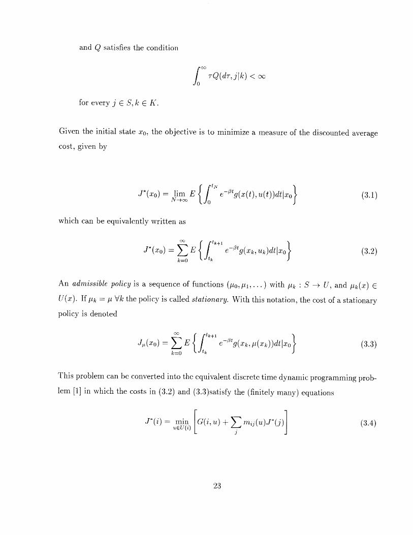
This problem can be converted into the equivalent discrete time dynamic programming prob-

lem [1] in which the costs in (3.2) and (3.3)satisfy the (finitely many) equations

J*(i) = minuEU(i)

G(i, u) + mij(u)J*(j)J

(3.3)

(3.4)

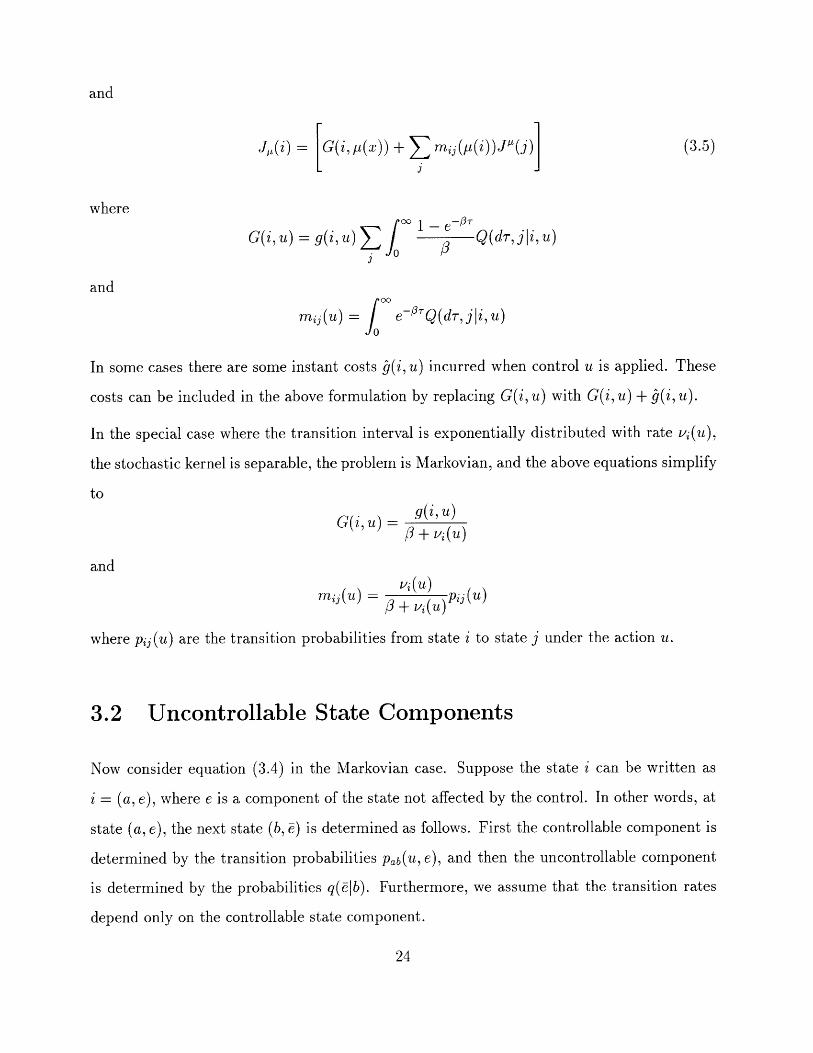
and

J,(i) = [G(ip(x)) + mi(p(i))J"(j) (3.5)

where

G(i, u) g(i, u) Q (d ji, a)

and

ms/(u) = J e-'Q(dT, ji, u)

In some cases there are some instant costs g(i, u) incurred when control u is applied. These

costs can be included in the above formulation by replacing G(i, u) with G(i, u) + g(i, u).

In the special case where the transition interval is exponentially distributed with rate vi(u),

the stochastic kernel is separable, the problem is Markovian, and the above equations simplify

toS g(i,u)

G(, u) = ()u +Vi (U)

and

m(u)= Pi ( (U)S+ Vi(u)

where pij(u) are the transition probabilities from state i to state j under the action u.

3.2 Uncontrollable State Components

Now consider equation (3.4) in the Markovian case. Suppose the state i can be written as

i = (a, e), where e is a component of the state not affected by the control. In other words, at

state (a, e), the next state (b, e) is determined as follows. First the controllable component is

determined by the transition probabilities Pab(u, e), and then the uncontrollable component

is determined by the probabilities q(elb). Furthermore, we assume that the transition rates

depend only on the controllable state component.

By setting J(i) = - q(e a)J*(a, e). Then equation (3.4) can be written as

J(a)= q(ela) minuEU(a,e)

G(a, e, u)+ V Pab(u,

J

In the problem treaded in this thesis, some more simplifications are possible and will be

discussed in the next chapter.

)J(b) (3.6)

Chapter 4

Problem Formulation

4.1 Formulation of the Problem as a Markov Decision

Process

In this section the call admission and channel allocation problem is formulated as a continuous

time controlled Markov process. The discounted cost to be minimized is the negative of the

number of users in the system, plus the instant penalties incurred if a call is blocked or

dropped.

Assume a cellular network with N cells and M channels. The state of the system is fully

described by the pair (A, e), where A is the occupancy matrix defined as

1 if channel j is used in cell i,

0 otherwise.

and e denotes the current event. The current event may be an arrival, a departure, or a

handoff request. This component of the state is uncontrollable.

The arrival processes in each cell are independent, Poisson with parameter Ai, where i is the

cell number. The holding time in each cell, that is the time before either a departure or a

handoff request, is exponentially distributed with mean 1/yu for all the cells. The probability

of a handoff from cell i to cell j is given by pij.

The problem belongs to the class of continuous time controlled Markov processes with un-

controllable state components, so equation (3.6) of the previous section applies. The equation

can be simplified further because the transition rates do not depend on the control, and the

next state is deterministic. In particular, VA(U) = VA and PAA(u) = 6(A, f(A, e, u)).

where (x, y) =1 if x = y,

0 otherwise

and f(A, e, u) is a deterministic function that uniquely determines the next state.

With these simplifications equation (3.6) reduces to

+A J(A)=+ V q(ejA) minuCU(A,e)

G(A, e, u) + -A J(f(A,e,+ V

The transition rates VA and the probabilities q(elA) can be computed by the system para-

meters as follows:

Define mi = E - A- = number of channels occupied in cell i.

m = E mi = number of channles occupied in the system.

Also let pi = k Pik, where the sum is over the neighbors of cell i.

The transition rate out of a state A is given by

VA A j + my (4.2)j=1

The transition probabilities q(efA) at each state can be expressed as a function of these

numbers.

u)) (4.1)

Pr{Next event is an arrival at cell klA} = fk (4.3)VA

Pr{Next event is a departure from channel j of cell k|A} = (1 - Pk)pAkj (4.4)VA

Pr{Next event is a handoff from channel j of cell i to cell kA} = ,LPik (4.5)VA

4.2 Motivation and Implementation

Even for relatively small cellular networks, the state space is too large to allow analytical or

exact computational solutions. Just a 10-cell, 10-channel system has a state space of approx-

imately 2100 _ 1.27 - 1030 states and the systems typically considered are much larger than

that. For that reason the problem has been mostly attacked by well thought out heuristics.

The idea of obtaining channel assignment strategies by minimizing a cost function has been

reported in [9], where a heuristically derived energy function is used and trained by means

of a neural network architecture, and in [19] where a Markov decision model is used and the

cost-to-go is approximated by a compact representation architecture. This is the approach

adopted in this thesis.

The N cells of the system are assumed to be arranged in a two dimensional array of hexagonal

blocks, of horizontal dimension Nh, and vertical dimension N,. Each cell has an equal number

M of channels assigned. Throughout the network there is a fixed reuse distance of r cells.

There is no predefined set of channels that a cell can use (as in fixed assignment strategies).

Every channel can be used in the cell provided that the reuse constraints are not violated.

Random events are generated from a random distribution with the probabilities described.

The control actions available in the present implementation are described below.

* Upon a new call arrival, the available control actions are to accept or reject the call

(in the call admission problem) and to allocate a channel if the call is accepted (in the

channel allocation problem). The decision to accept is available only if there exists

at least one free channel, and the channel assignment decision is subject to the reuse

constraints of the network.

* Upon a a call departure, the available set of actions is to perform a channel rearrange-

ment in the cell from which the call departed. The set of rearrangements available is

moving a call from an occupied channel to the channel that has just been freed.

* Upon handoff from one cell to the other, the set of decisions is the following. If the call

cannot be accepted due to channel unavailability it departs and a channel rearrangement

is performed in the cell from which the handoff was initiated. Otherwise, each free

channel is considered for accepting the call while simultaneously a rearrangement is

performed (if possible) in the cell from which the handoff was initiated.

Given the current event e, and a control action u the next state is uniquely determined and

denoted f(A, e, u). In the neuro-dynamic programming approach the decision is chosen by

the control u that minimizes the approximate cost-to-go.

u =arg min {g(A, e, u) + J(f(A, e,u))uEUA

In the above equation a = 1O+V"

In the current implementation, the approximation j is a linear architecture of features. Differ-

ent sets of features were used and compared for both the channel allocation and the admission

control problem. A number of heuristic controllers were also implemented for comparison.

These controllers use some predefined strategy to select decisions. The performance of the

controllers was measured by the blocking and dropping rates attained by the system.

4.3 The Channel Allocation Problem without Handoffs

In the simple channel allocation problem without admission control, the handoff probabilities

pij are set to 0 and the only events that can occur are arrivals and departures. The decision

set differs from the one just described in that upon a new call arrival the option to reject is

no longer available, and the only option considered is the call placement (provided that there

are free channels in the cell).

The initial set of features implemented is the one used in [19].

1. An availability feature. For each cell i the feature Fi is defined by Fi(A) = number of

free channels in cell i. This feature attempts to capture the ability of the system to

accept new calls.

2. A packing feature for each (cell,channel) pair. For each cell i and channel c the feature

fi,, is defined by fi,,(A) = number of times channel c is reused in a radius from cell i

equal to the reuse distance of the system. This feature attempts to capture the efficiency

with which channels are reused in the system.

The results obtained in [19] show that the performance of the approximate dynamic program-

ming method was better than the performance of BDCL which is one of the best available

heuristic algorithms [8]. It turns out that the performance of the neuro-dynamic approach

is very close to the performance of the heuristic algorithm that selects a channel such that

the total number of free channels in the system is maximized. This is one the of best known

heuristics for the channel assignment problem and it is used in this thesis for comparison

throughout the experiments.

4.3.1 Description of Training Parameters and Experimental Results

The first implementation uses the features described and is trained by TD(A) . The para-

meters of the implementation are briefly discussed.

Discount Factor The discount factor a defined as a = " is set to 0.995, in order forf+v

future rewards to weight considerably. Experiments with lower values of a were also

implemented but the results were almost identical.

Initial State The initial state is throughout an empty system. It is a non-representative

state, but the process transitions very fast from the uninteresting region of a nearly

empty system to a nearly full and consequently the cost samples collected in the initial

phases are insignificant.

Initial Weights Initially, negative weights were used for the features associated with the

free channels. It turns out that the initial choice of weights was of small importance in

this particular version of the problem.

Step-size Rule The step-size rule used is of the form yt = - where yo is an initial value

and t is increased by 1 every 1000 iterations. Training is particularly sensitive to the

choice of the initial value of the step-size which depends in an unpredictable fashion on

the number of features and the size of the system.

Value of A The default value for A in all the tests is 0. Other values of A where tested and

compared.

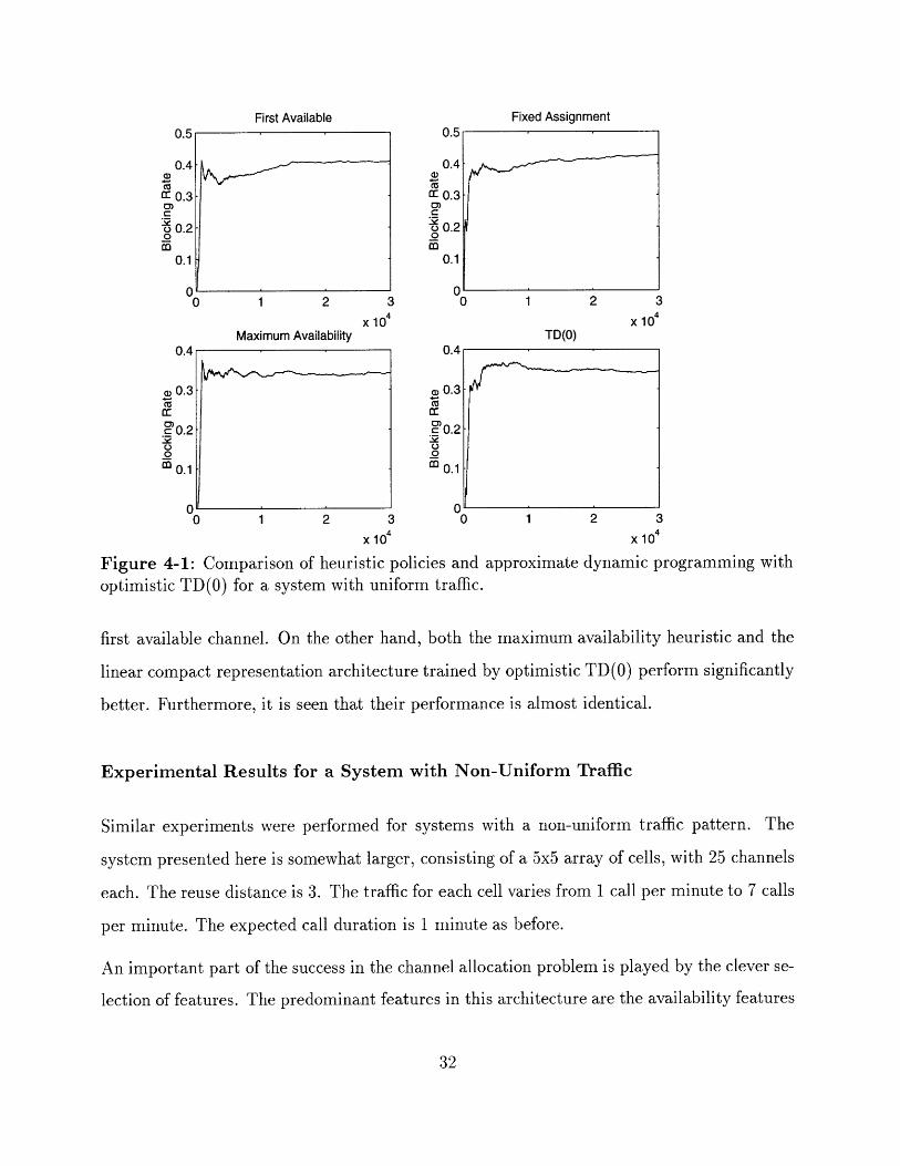
Experimental Results for a System with Uniform Traffic

Several simulations were performed for large and small systems under light and heavy traffic

conditions. The results presented here are for a 4x4 array of cells with 16 channels in each

cell. The reuse distance is 2. The arrival rate is 4 calls per minute uniformly throughout

the system and the average call duration time is 2 minutes. The performance measure is the

steady state blocking rate of the algorithm. Figure 4-1 illustrates the relative performance

of the approximate dynamic programming approach compared to the performance of some

heuristics.

The optimal fixed assignment strategy, under which 4 channels are assigned to each cell, does

not perform any better than the simplest dynamic assignment strategy which is to assign the

Firt valaleFixd ssgnen

C

¢r

oo

m

0.0

0.4

caCC 0.3C

3 0.2o

0.1

n

0 1 2 3

x 104 x 104

Maximum Availability TD(0)

0 1 2 3

x 104 X 104

Figure 4-1: Comparison of heuristic policies and approximate dynamic programming withoptimistic TD(O) for a system with uniform traffic.

first available channel. On the other hand, both the maximum availability heuristic and the

linear compact representation architecture trained by optimistic TD(O) perform significantly

better. Furthermore, it is seen that their performance is almost identical.

Experimental Results for a System with Non-Uniform Traffic

Similar experiments were performed for systems with a non-uniform traffic pattern. The

system presented here is somewhat larger, consisting of a 5x5 array of cells, with 25 channels

each. The reuse distance is 3. The traffic for each cell varies from 1 call per minute to 7 calls

per minute. The expected call duration is 1 minute as before.

An important part of the success in the channel allocation problem is played by the clever se-

lection of features. The predominant features in this architecture are the availability features

Fixed AssignmentFirst Available

Cz

0r

oirn

(~

Maximum AvailabilityU.0

0.4(a

Cr 0.3C

5 0.2o

0.1

n0 1 2 3 4 0 1 2 3 4

x104 X 104

TD(0) with All the Features TD(0) with Free Channels as Features

a'CU

0)

0oO

x 10 4 X 10 4

Figure 4-2: Comparison of heuristic policies and approximate dynamic programming withoptimistic TD(O) for a system with non-uniform traffic.

that count the free channels in each cell. An architecture with only these features should

be able to perform as well as the maximum availability heuristic, although the number of

parameters is small. This suggests that an architecture with good features can give good

performance even if it has only a few parameters. Indeed, this hypothesis was tested by

creating an architecture that uses only the free channels per cell as a feature. In figure 4-2

these two architectures are compared with the First Available and the Maximum Availability

heuristics.

It is seen that the performance of the maximum availability heuristic and the architecture

with the free channels feature are almost identical. The full powered architecture performs

only a trifle better.

First Available,,

- v

0 1 2 3 4 0 1 2 3 4x 104

x 104

TD(0) with All the Features TD(0) with Free Channels as Features

r r

Varying the Value of A

It is shown in [3] that TD(A) with a linear architecture converges under the following condi-

tions.

1. The step-sizes yt are positive, deterministic, and satisfy E-t 7t = c0 and Et=0 7t2 <

00.

2. The underlying Markov chain corresponding to the policy being evaluated is aperiodic

and has a single recurrent class.

3. There are fewer parameters than states and the features are linearly independent.

This result establishes the validity of approximate policy iteration. The performance bound

obtained under the above assumptions deteriorates as the value of A decreases. This suggests

that values of A that are close to 1 will attain better performance. There are no convergence

guarantees for optimistic policy iteration but it often used in large problems because, when

it converges, it converges much faster than non-optimistic policy iteration. The performance

varies as a function of A but not consistently with the theory for approximate policy iteration.

Determining the best value for A is a matter of trial and error. In the following table, the

setup of the non-uniform traffic problem is used to compare different values of A.

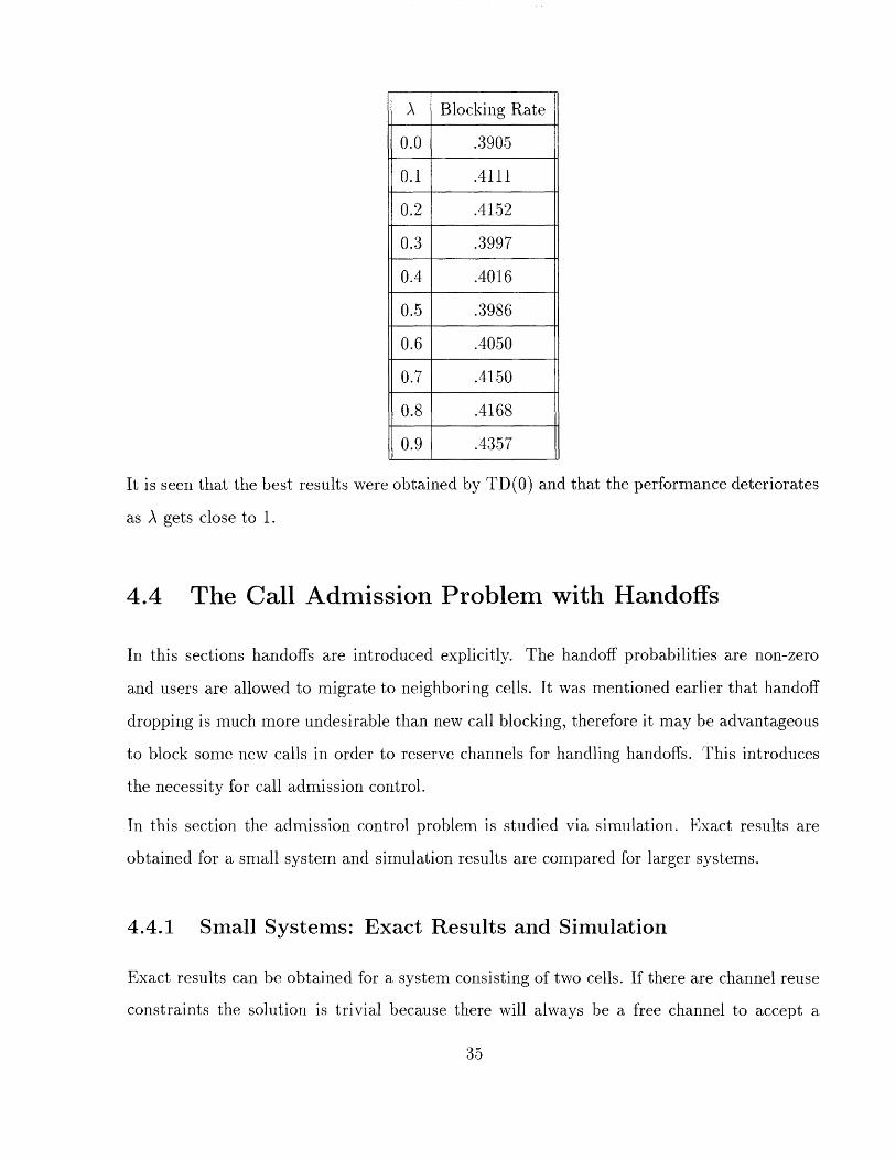
It is seen that the best results were obtained

as A gets close to 1.

by TD(0) and that the performance deteriorates

4.4 The Call Admission Problem with Handoffs

In this sections handoffs are introduced explicitly. The handoff probabilities are non-zero

and users are allowed to migrate to neighboring cells. It was mentioned earlier that handoff

dropping is much more undesirable than new call blocking, therefore it may be advantageous

to block some new calls in order to reserve channels for handling handoffs. This introduces

the necessity for call admission control.

In this section the admission control problem is studied via simulation. Exact results are

obtained for a small system and simulation results are compared for larger systems.

4.4.1 Small Systems: Exact Results and Simulation

Exact results can be obtained for a system consisting of two cells. If there are channel reuse

constraints the solution is trivial because there will always be a free channel to accept a

A Blocking Rate

0.0 .3905

0.1 .4111

0.2 .4152

0.3 .3997

0.4 .4016

0.5 .3986

0.6 .4050

0.7 .4150

0.8 .4168

0.9 .4357

handoff (namely the channel from which the handoff departed). Therefore it is interesting to

focus on the system without reuse distance constraints.

The study of this small system gives important insights on the form of the optimal policy as

well as its dependence on the parameters of the problem. Some insights can also be obtained

on things that can go wrong with simulation and training.

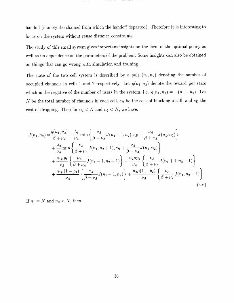
The state of the two cell system is described by a pair (ni, n2 ) denoting the number of

occupied channels in cells 1 and 2 respectively. Let g(ni, n2) denote the reward per state

which is the negative of the number of users in the system, i.e. g(nl, n2) = -(nl + n2). Let

N be the total number of channels in each cell, cB be the cost of blocking a call, and cD the

cost of dropping. Then for nl < N and n2 < N, we have.

g(nl,n 2 ) Amin VA J(nl +1,2), CB + VA J(n, n 2 )}

+ J(n min (n, n2 + 1), cB + J(n, n2

VA VA VA

+ { VA J(ni - 1, n 2 1)2/P { -A (n 1, n2- 1)VA +VA VA VA

_+_ n - Pi) +AA J(n - 1, n2) + n 2C1(1 - p 2 ) -A J(nln2 -1)}

VA VA VA VA

(4.6)

If nl = N and n2 < N, then

J(I 2)-- g(nI, n2)J(121 , 2)

/ + VA

+ - min/VA

3+A J(ni, n 2 +13 -J t/A

+ nipp1 i VAVA + VA

npll(1 - Pi) {CDVAD

1 - 1, n2 + 1

VAP+V1

) n2+ P2VA

-1,n 2) +

VA

n221(1 - P2)

VA

1,n2 - 1)}

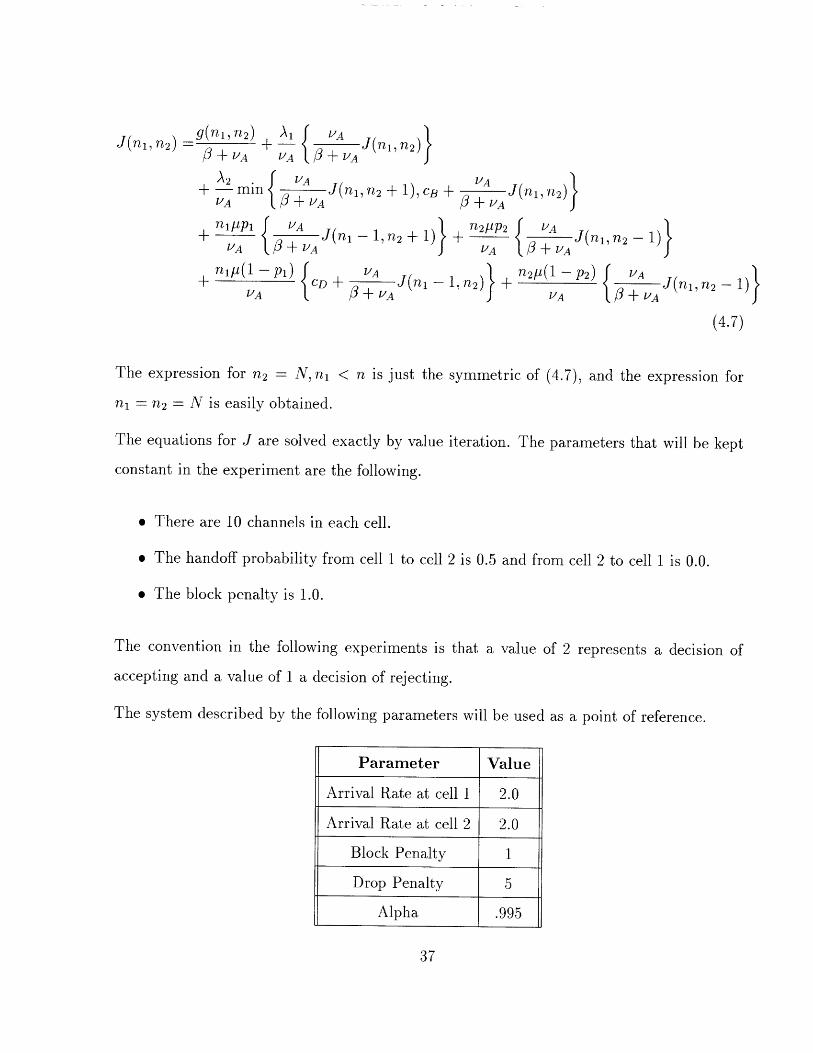
(4.7)

The expression for n2 = N, nl < n is just the symmetric of (4.7), and the expression for

nl = n2 = N is easily obtained.

The equations for J are solved exactly by value iteration. The parameters that will be kept

constant in the experiment are the following.

* There are 10 channels in each cell.

* The handoff probability from cell 1 to cell 2 is 0.5 and from cell 2 to cell 1 is 0.0.

* The block penalty is 1.0.

The convention in the following experiments is that a value of 2 represents a decision of

accepting and a value of 1 a decision of rejecting.

The system described by the following parameters will be used as a point of reference.

A VA (ni, 2)VA + VA

C+ A J(ni, n2)}1 3 + VA

Parameter Value

Arrival Rate at cell 1 2.0

Arrival Rate at cell 2 2.0

Block Penalty 1

Drop Penalty 5

Alpha .995

Arrival Rate at Cell 1: 2.0Arrival Rate at Cell 2: 2.0Block Penalty: 1Drop Penalty: 5Alpha: 0.995

Decision for Arrivals at cell 1 Decision for Arrivals at 2

10

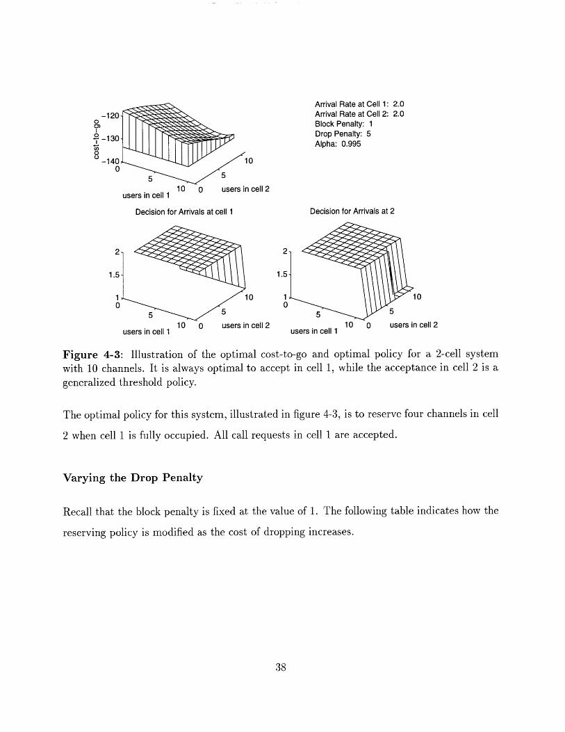
Figurewith 10

4-3:

10 0 users in cell 2 10 0 users in cell 2,ers in cell 1 users in cell 1

Illustration of the optimal cost-to-go and optimal policy for a 2-cell systemchannels. It is always optimal to accept in cell 1, while the acceptance in cell 2 is a

generalized threshold policy.

The optimal policy for this system, illustrated in figure 4-3, is to reserve four channels in cell

2 when cell 1 is fully occupied. All call requests in cell 1 are accepted.

Varying the Drop Penalty

Recall that the block penalty is fixed at the value of 1. The following table indicates how the

reserving policy is modified as the cost of dropping increases.

-120o

S-130

-1400

10

n cell 2

US

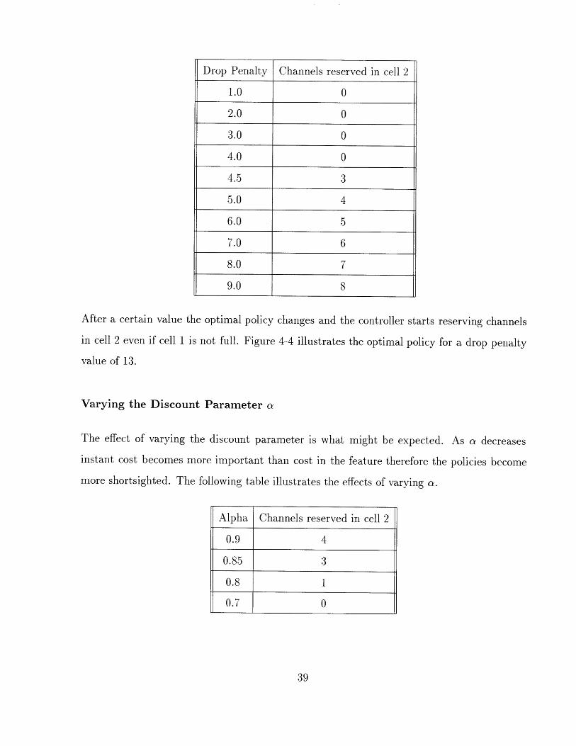
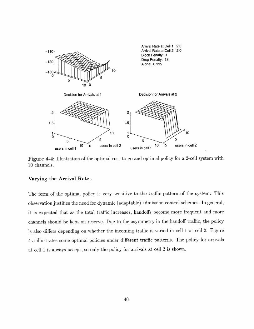
After a certain value the optimal policy changes and the controller starts reserving channels

in cell 2 even if cell 1 is not full. Figure 4-4 illustrates the optimal policy for a drop penalty

value of 13.

Varying the Discount Parameter a

The effect of varying the discount parameter is what might be expected. As a decreases

instant cost becomes more important than cost in the feature therefore the policies become

more shortsighted. The following table illustrates the effects of varying a.

Drop Penalty Channels reserved in cell 2

1.0 0

2.0 0

3.0 0

4.0 0

4.5 3

5.0 4

6.0 5

7.0 6

8.0 7

9.0 8

Alpha Channels reserved in cell 2

0.9 4

0.85 3

0.8 1

0.7 0

Arrival Rate at Cell 1: 2.0Arrival nate at Cell 2: 2.uBlock Penalty: 1Drop Penalty: 13Alpha: 0.995

10

Decision for Arrivals at 1 Decision for Arrivals at 2

2

1.5

10

2

1.5

0 10

10

10 0 users in cell 2 10 0 users in cell 2users in cell 1 users in cell 1

Figure 4-4: Illustration of the optimal cost-to-go and optimal policy for a 2-cell system with10 channels.

Varying the Arrival Rates

The form of the optimal policy is very sensitive to the traffic pattern of the system. This

observation justifies the need for dynamic (adaptable) admission control schemes. In general,

it is expected that as the total traffic increases, handoffs become more frequent and more

channels should be kept on reserve. Due to the asymmetry in the handoff traffic, the policy

is also differs depending on whether the incoming traffic is varied in cell 1 or cell 2. Figure

4-5 illustrates some optimal policies under different traffic patterns. The policy for arrivals

at cell 1 is always accept, so only the policy for arrivals at cell 2 is shown.

11 = 1.0, 12 = 2.0

21

1 x

05

10 0

11 = 4.0, 12 = 2.0 11 = 2.0, 12 = 4.0

2

1

0 00

Figure 4-5: Illustration of the optimal cost-to-go and optimal policy for a 2-cell system with10 channels under different traffic patterns. The arrival rate at cell 1 is given by 11 and therate at cell 2 by 12.

Some Simulation Results for the Small System

Now some sample simulation runs with this small system are presented. The architecture

used is linear in the following features.

* The free channels feature described earlier.

* The times a channel is reused feature also described earlier.

* The probability of handoff in cell 2, which is 0 if cell 1 is empty and 0.5 if it is occupied.

Figure 4-6 shows the considerable advantage of the optimal policy over policies that reserve a

fixed number of channels in the second cell irrespectively of the number of occupied channels

in cell 1.

11 = 2.0, 12 = 1.0

O,0

0.1

0.05

n

.UV4

0.03

0.02

0.01

0 0.2 0.4 0.6 0.8 1 1.2 1.4 1.6 1.8 2x 104

0 0.2 0.4 0.6 0.8 1 1.2 1.4 1.6 1.8 2

x 104

Figure 4-6: Comparison of the performance of the optimal policy, against the performanceobtained by channel reserving heuristics. The upper graph is the blocking rate and the lower

the dropping rate of the system.

A number of experiments are performed in order to evaluate a) the ability of the method

to learn a good policy and b) the power of the architecture. In the first experiment, that

is designed to test the ability of the method to learn good policies, training starts with the

initial weights set at 0. In the second experiment, that is designed to test the power of the

architecture, good initial weights are used. In particular, the second experiment works as

follows: The controller is using the optimal policy described earlier to make decisions and the

parameters (weights) are trained on the decisions made but this policy. Therefore, at the end

of the simulation run the final weights must provide a good parameterization of the optimal

policy. If the optimal policy is adequately represented then the greedy policy with respect to

this parameterization should match the optimal policy. Otherwise, the greedy policy will be

worse or just as good.

4I I I I I I I

Ili --' -'\ I '

-- -.. . .--. - -- --

N

I I I I I I

solid line: optimal policy_ -- : policy of reserving 2 channels

.- : policy of reserving 3 channels

i \

S-- --- - - ----

C15

tj0 0.2 0.4 0.6 0.8 1 1.2 1.4 1.6 1.8 2x 104

Optimistic Policy IterationU.0

0.4

0.3

0.2

0.1

n

U.U1 I

0.0

0.00

0 0.2 0.4 0.6 0.8 1 1.2 1.4 1.6 1.8 2

x 104

0 0.2 0.4 0.6 0.8 1 1.2 1.4 1.6 1.8 2

x 104

Figure 4-7: Results obtained with optimistic policy iteration with different sets of initialweights.The upper graph is the blocking rate and the lower the dropping rate of the system.

Figures 4-7 and 4-8 illustrate the results of these experiments with an architecture trained

by optimistic and approximate policy iteration respectively.

The initial policies obtained with both optimistic and approximate policy iterations are way

off the optimum. Moreover, the approximate policy iteration oscillates between policies that

reject far too often. However, when started with good weights the performance is close to

optimal but doesn't match it exactly. This suggests that the ability of the method to learn

good policies is weak and that the architecture can adequately, but not exactly, represent the

optimal policy.

A few remarks are in order here regarding the performance of non-optimistic policy iteration.

The behavior shown in figure 4-8 has been encountered in many simulation runs, in both

small and large systems. The reason that approximate policy iteration jumps from to a highly

rejecting policy is probably due to the poor initial weights. The reason why it doesn't learn

solid line: training with 0 initial weights

olittd line: training with good initial weights

-- dotted line: training with good initial weights

' .. , -. ..

n,

Approximate Policy IterationU.4

0.3

0.2

0.1

0

0.2

0.15

0.1

0.05

n

0 0.2 0.4 0.6 0.8 1 1.2 1.4 1.6 1.8 2

x 104

0 0.2 0.4 0.6 0.8 1 1.2 1.4 1.6 1.8 2

x 104

Figure 4-8: Results obtained with approximate policy iteration with different sets of initialweights.The upper graph is the blocking rate and the lower the dropping rate of the system.

to perform better is the following: Under a policy that rejects often, states where cells are

heavily occupied are never visited. Therefore the samples obtained are only from a limited,

non-representative number of states and therefore the cost-to-go approximation obtained is

poor and results in a similarly bad policy. Once a highly rejecting policy is reached, the

method will go on oscillating between bad policies.

Conclusions of this Section

The insights gained by the results of this section are summarized here.

1. It appears that under any combination of block/drop penalties, the optimal policy is not

to reserve a fixed number of channels in a cell irrespectively of how many channels are

occupied in the neighbors. This suggests that better performance than that of simple

I-- - I I -

-f

^^

v0 0.2 0.4 0.6 0.8 1 1.2 1.4 1.6 1.8 2x 104

_

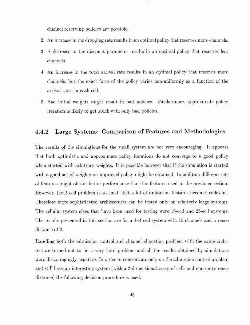
channel reserving policies are possible.

2. An increase in the dropping rate results in an optimal policy that reserves more channels.

3. A decrease in the discount parameter results in an optimal policy that reserves less

channels.

4. An increase in the total arrival rate results in an optimal policy that reserves more

channels, but the exact form of the policy varies non-uniformly as a function of the

arrival rates in each cell.

5. Bad initial weights might result in bad policies. Furthermore, approximate policy

iteration is likely to get stuck with only bad policies.

4.4.2 Large Systems: Comparison of Features and Methodologies

The results of the simulations for the small system are not very encouraging. It appears

that both optimistic and approximate policy iterations do not converge to a good policy

when started with arbitrary weights. It is possible however that if the simulation is started

with a good set of weights an improved policy might be obtained. In addition different sets

of features might obtain better performance than the features used in the previous section.

However, the 2 cell problem is so small that a lot of important features become irrelevant.

Therefore more sophisticated architectures can be tested only on relatively large systems.

The cellular system sizes that have been used for testing were 16-cell and 25-cell systems.

The results presented in this section are for a 4x4 cell system with 16 channels and a reuse

distance of 2.

Handling both the admission control and channel allocation problem with the same archi-

tecture turned out to be a very hard problem and all the results obtained by simulations

were discouragingly negative. In order to concentrate only on the admission control problem

and still have an interesting system (with a 2-dimensional array of cells and non-unity reuse

distance) the following decision procedure is used.

Suppose that the system is in state A. Upon a call arrival, the channel that will accept the

call is decided with the maximum availability heuristic. The approximate cost-to-go of the

resulting state, A, is computed and the call is accepted if aJ(A) < Blocking Cost + aJ(A).

Upon handoffs and departures, the channel allocation and rearrangement decisions are also

made with the maximum availability heuristic, so there is no choice of actions when these

events occur.

Features

The following is a list of features that were implemented and their description.

1. Free channels This is the feature described in section 4.3, that counts the free channels

in each cell.

2. Number of times a channel is reused This feature is also described in section 4.3.

3. Handoff probability This feature is a measure of the probability of a handoff in a cell

i. For each neighbor j the number of users mj is computed and the feature has the

value E jpj', where the summation is over the neighbors of i.

4. Drop probability This feature is the probability that a cell will be dropped in cell i,

given that the next event is a handoff into i. It provides a measure of the danger of an

imminent drop.

5. Used channels This is just the average reward and can be used either as a cell by cell

feature or as a global feature. The reason that the reward has been chosen to serve as

a feature is the following: The choice of the magnitude of the drop and block penalties

is arbitrary and it might be the case that their accumulative effect is so mush larger

than the effect of average rewards, so that the training method does not "recognize" the

necessity of keeping a large number of users. In some simulations this feature resulted

in a performance improvement.

The architectures compared in this section are composed of combinations of the features

described. Other features were also tested but resulted in poor performance.

Simulation Results for a System with Uniform Handoff Probability

For easy reference the architectures will be denoted by sets of numbers that correspond to

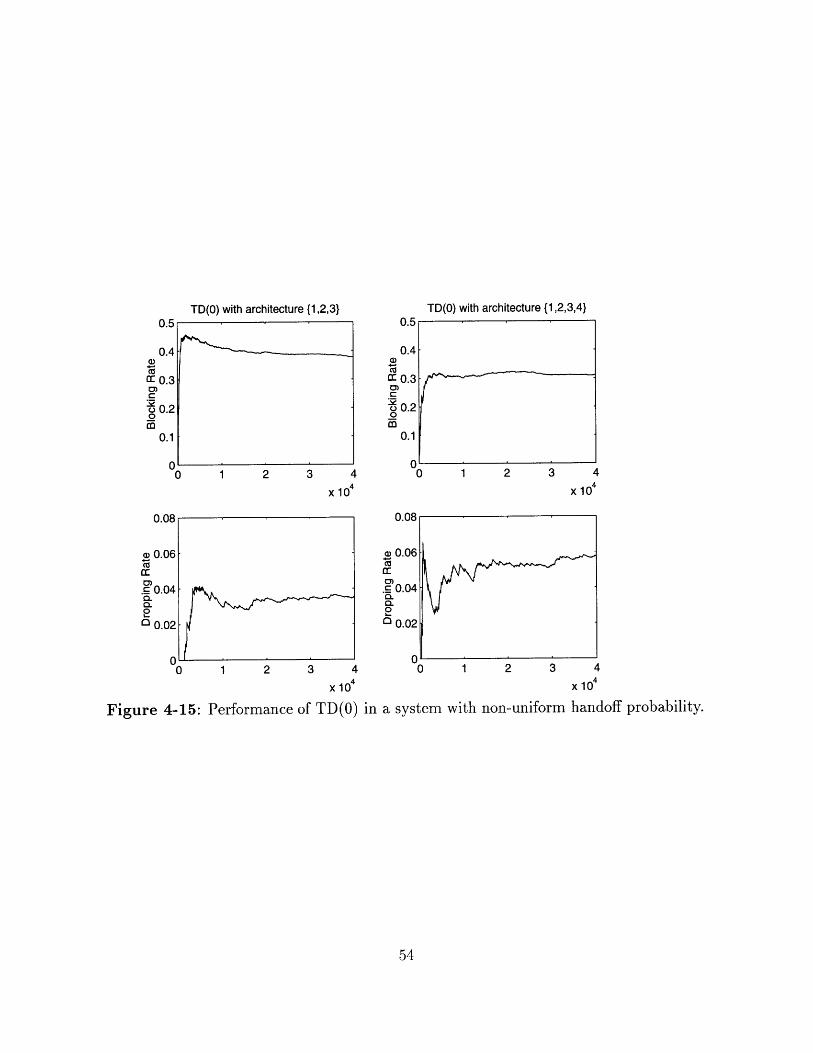
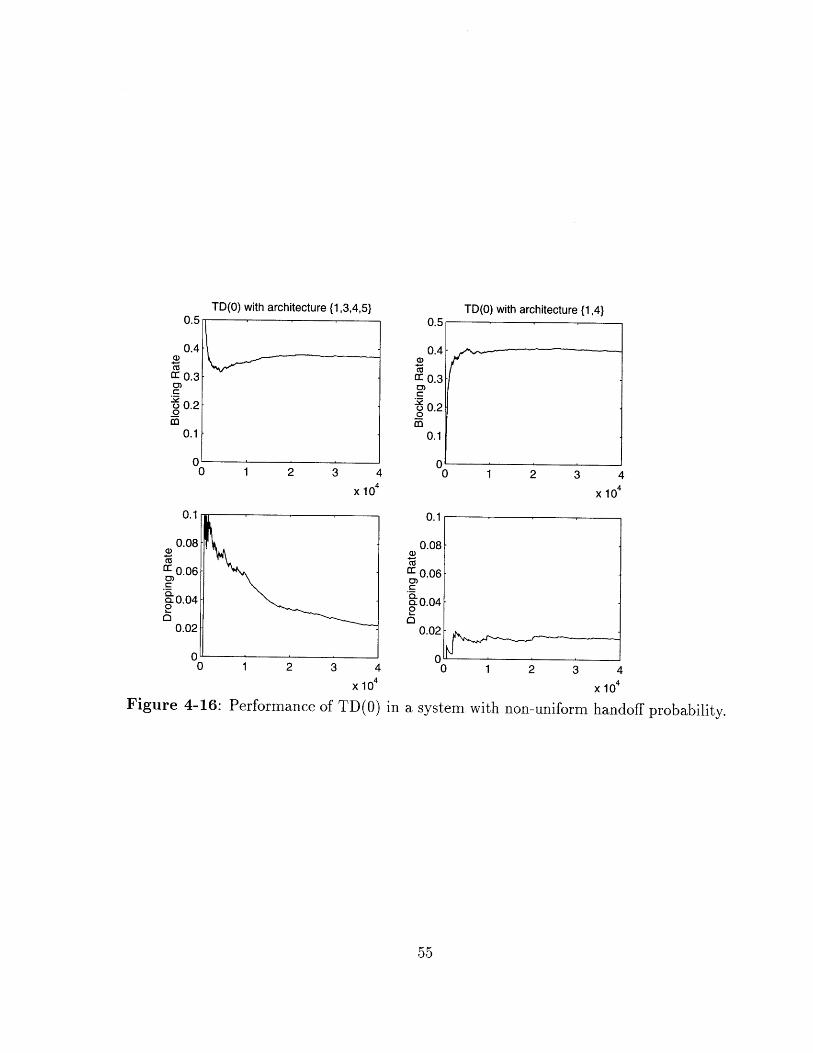
the features described. The architectures discussed here are {1,2,3}, {1,2,3,4}, { 1,3,4,5}, and

{1,4}.

The heuristic against which these architectures are compared is described by the following

strategy.

* All allocation and rearrangement decisions are made by the maximum availability heur-

istic.

* A new call request is rejected if the cell in which the call arrives has less free channels

than a prespecified fixed number.

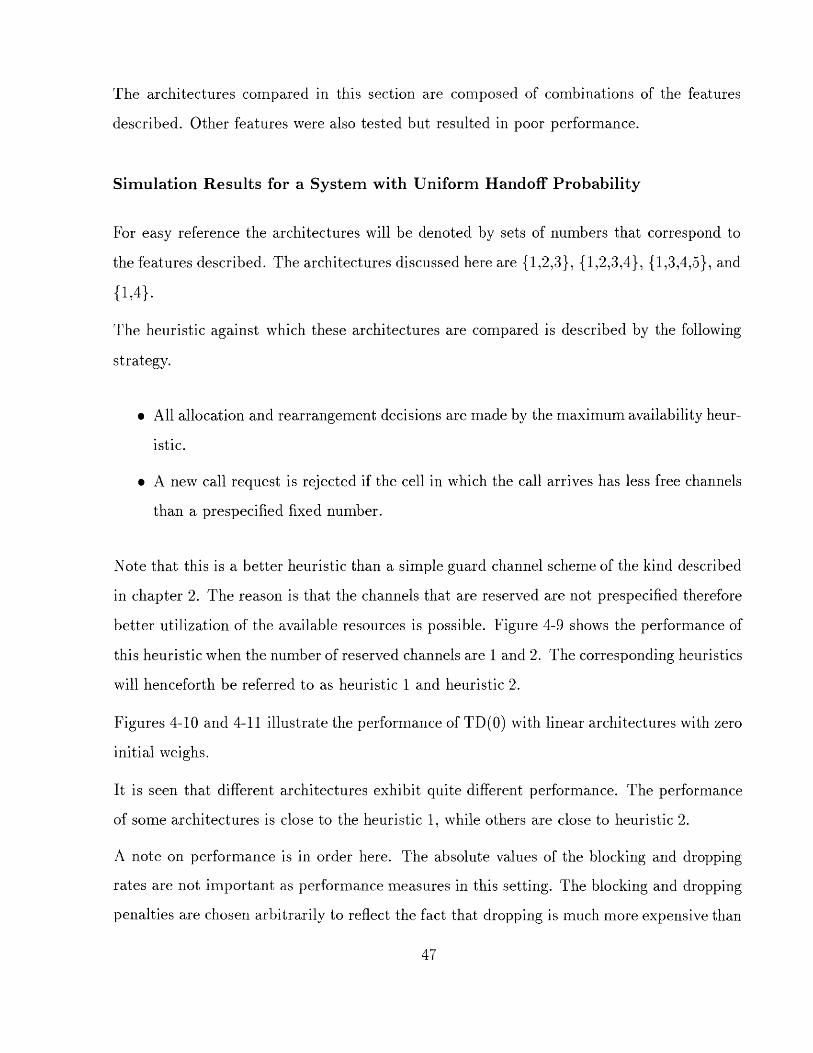
Note that this is a better heuristic than a simple guard channel scheme of the kind described

in chapter 2. The reason is that the channels that are reserved are not prespecified therefore

better utilization of the available resources is possible. Figure 4-9 shows the performance of

this heuristic when the number of reserved channels are 1 and 2. The corresponding heuristics

will henceforth be referred to as heuristic 1 and heuristic 2.

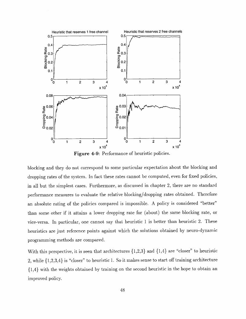
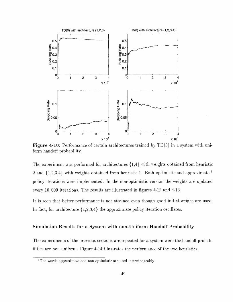
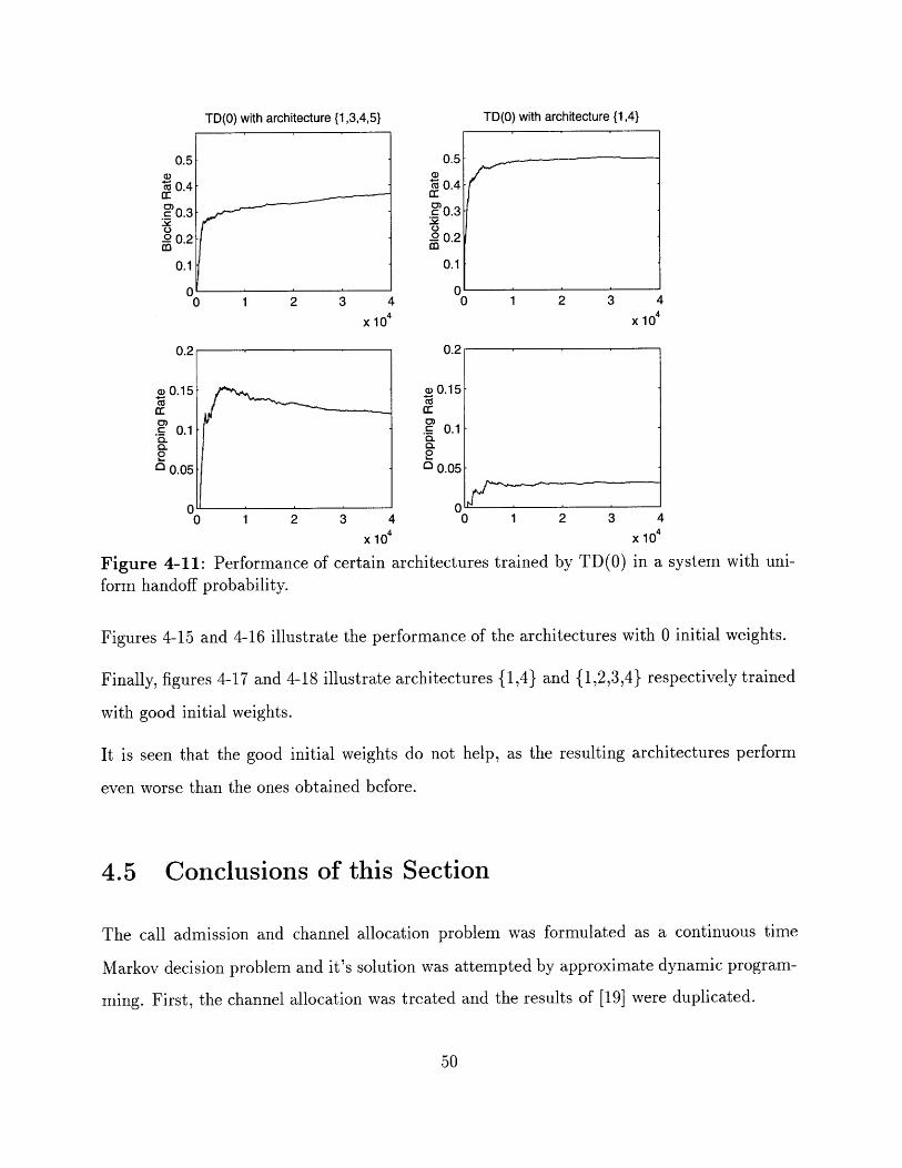
Figures 4-10 and 4-11 illustrate the performance of TD(0) with linear architectures with zero

initial weighs.

It is seen that different architectures exhibit quite different performance. The performance

of some architectures is close to the heuristic 1, while others are close to heuristic 2.

A note on performance is in order here. The absolute values of the blocking and dropping

rates are not important as performance measures in this setting. The blocking and dropping

penalties are chosen arbitrarily to reflect the fact that dropping is much more expensive than

Heuristic that reserves 2 free channelsU.0

0.4Ca

0.3

S0.2om

0.1

n0 1 2 3 4

x 104 x 104

1 2 3 4

x 104 x 104

Figure 4-9: Performance of heuristic policies.

blocking and they do not correspond to some particular expectation about the blocking and

dropping rates of the system. In fact these rates cannot be computed, even for fixed policies,

in all but the simplest cases. Furthermore, as discussed in chapter 2, there are no standard

performance measures to evaluate the relative blocking/dropping rates obtained. Therefore

an absolute rating of the policies compared is impossible. A policy is considered "better"

than some other if it attains a lower dropping rate for (about) the same blocking rate, or

vice-versa. In particular, one cannot say that heuristic 1 is better than heuristic 2. These

heuristics are just reference points against which the solutions obtained by neuro-dynamic

programming methods are compared.

With this perspective, it is seen that architectures {1,2,3} and {1,4} are "closer" to heuristic

2, while {1,2,3,4} is "closer" to heuristic 1. So it makes sense to start off training architecture

{1,4} with the weights obtained by training on the second heuristic in the hope to obtain an

improved policy.

Heuristic that reserves 1 free channel

v0 2 3 4

I

TD(0) with architecture {1,2,3,4}

0.5

ca 0.4Cc

r 0.32

S0.2

0.1

0 00 1 2 3 4

x 104 X 104

a,

2 0.050

n

a

a

U 1 2 4 U 1 z d 4

x 104 x 104

Figure 4-10: Performance of certain architectures trained by TD(0) in a system with uni-form handoff probability.

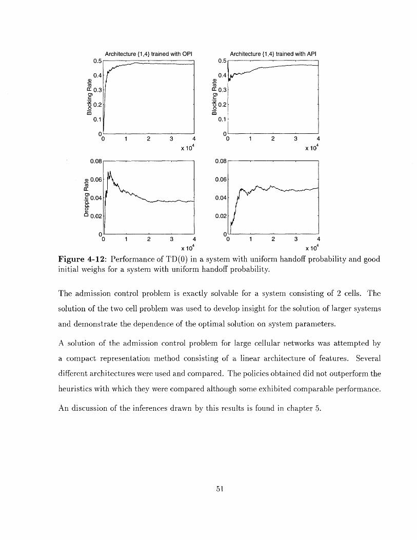
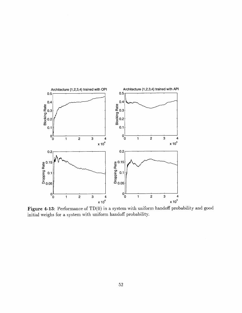
The experiment was performed for architectures {1,4} with weights obtained from heuristic

2 and {1,2,3,4} with weights obtained from heuristic 1. Both optimistic and approximate 1

policy iterations were implemented. In the non-optimistic version the weights are updated

every 10, 000 iterations. The results are illustrated in figures 4-12 and 4-13.

It is seen that better performance is not attained even though good initial weighs are used.

In fact, for architecture {1,2,3,4} the approximate policy iteration oscillates.

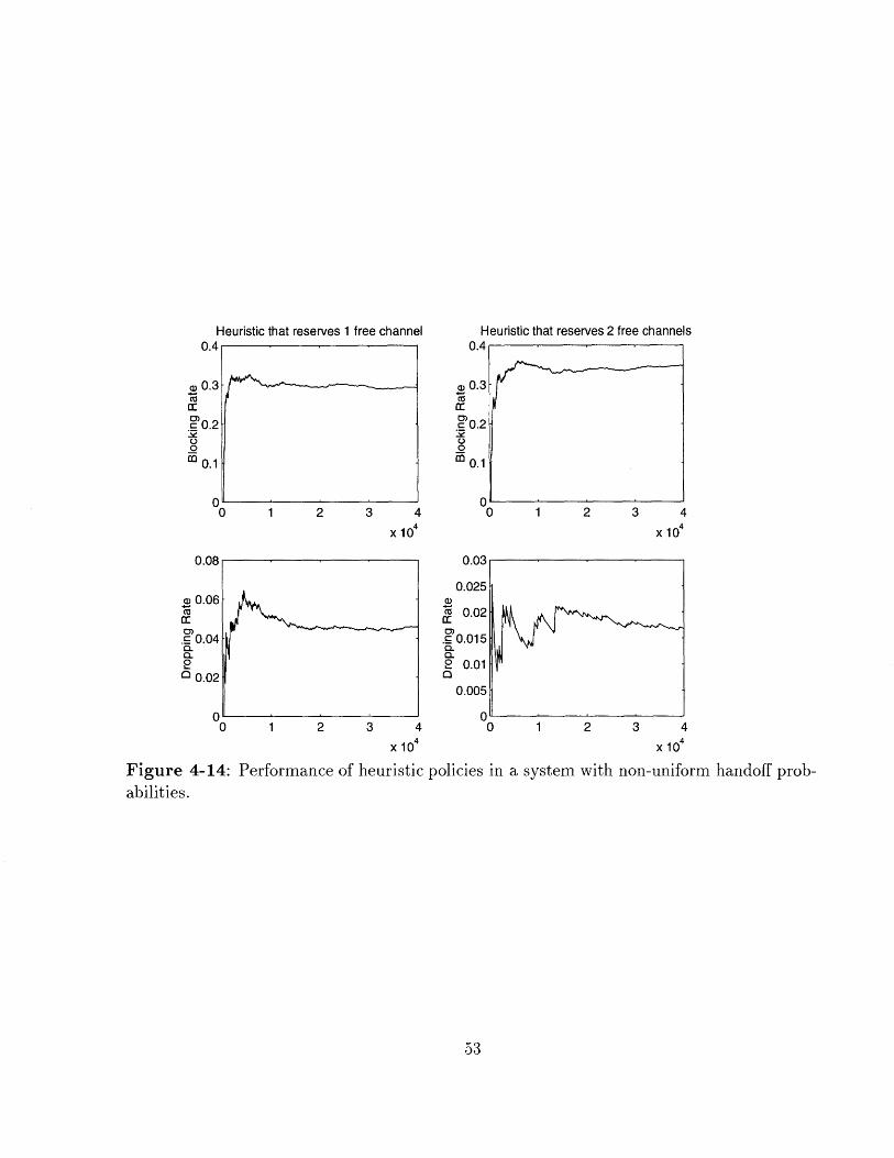
Simulation Results for a System with non-Uniform Handoff Probability

The experiments of the previous sections are repeated for a system were the handoff probab-

ilities are non-uniform. Figure 4-14 illustrates the performance of the two heuristics.

1The words approximate and non-optimistic are used interchangeably

TD(0) with architecture {1,2,3}

IrsJ_v

TD(0) with architecture {1,3,4,5}

U I 4

x 104 X 104

V0 1 2

Figure 4-11: Performanceform handoff probability.

0.1

a 0.15n"0.S0.1

C.a-

0oL.) 0.05

n

3 4 0 1 2 3 4

X 104 X 10 4

certain architectures trained by TD(O) in a system with uni-

Figures 4-15 and 4-16 illustrate the performance of the architectures with 0 initial weights.

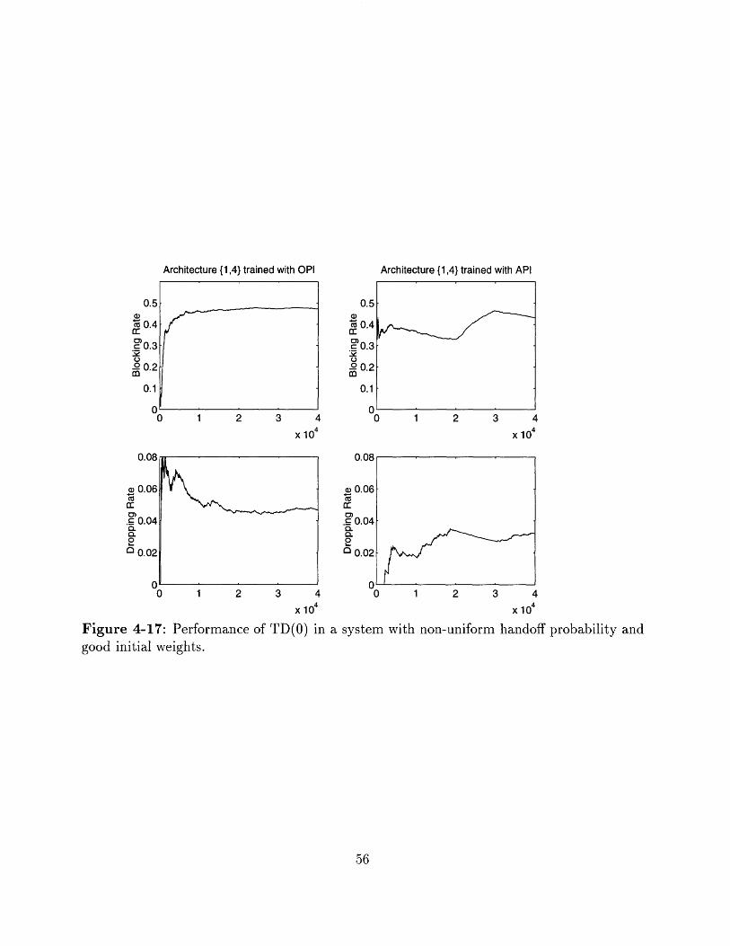
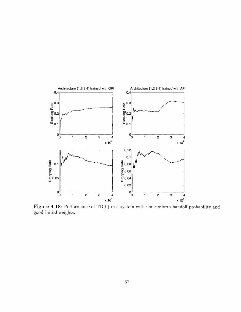
Finally, figures 4-17 and 4-18 illustrate architectures {1,4} and {1,2,3,4} respectively trained

with good initial weights.

It is

even

seen that the good initial weights do not help, as the resulting architectures perform

worse than the ones obtained before.

4.5 Conclusions of this Section

The call admission and channel allocation problem was formulated as a continuous time

Markov decision problem and it's solution was attempted by approximate dynamic program-

ming. First, the channel allocation was treated and the results of [19] were duplicated.

TD(0) with architecture {1,4}

!

I I J

Architecture (1,4} trained with OPI

1 2 3 4

x 10 4

0.5

0.4

rr0.3

S0.2

0.1

00 1 2 3 4

X 104

0 1 2 3 4 0 1 2

x 104

Figure 4-12: Performance of TD(0O) in a system with uniforminitial weighs for a system with uniform handoff probability.

The admission control problem is exactly solvable for a system consisting of 2 cells. The

solution of the two cell problem was used to develop insight for the solution of larger systems

and demonstrate the dependence of the optimal solution on system parameters.

A solution of the admission control problem for large cellular networks was attempted by

a compact representation method consisting of a linear architecture of features. Several

different architectures were used and compared. The policies obtained did not outperform the

heuristics with which they were compared although some exhibited comparable performance.

An discussion of the inferences drawn by this results is found in chapter 5.

0

U.b

0.4

0

0.1

r

U.U

. 0.00.

0.0

0

o 0.0

3 4

x 104

handoff probability and good

^ _

Architecture {1,4} trained with API-

1 -~-c~---

Architecture {1,2,3,4} trained with OPI

0.3

0.2

0.1

1 2 3 4

x 104

x 104

1 2 3 4

x 104

0 1 2 3 4

X 104

Figure 4-13: Performance of TD(O) in a system with uniform handoff probability and good

initial weighs for a system with uniform handoff probability.

C==

.o0

0.

~0.1

0

o 0.0

Architecture {1,2,3,4} trained with API

Heuristic that reserves 2 free channels

x 104 x 104

1 2 3 4 1 2 3 4

x 104 x 104

Figure 4-14:abilities.

Performance of heuristic policies in a system with non-uniform handoff prob-

0.

0.

oc

O.

Ca

cEC1

00'-0._=a3

Heuristic that reserves 1 free channel

a,

TD(O) with architecture {1,2,3,4}U.b

0.4

0.3

S0.2m

0.1

n

1 2 3 4

x 104

C 1 2 3 4

x 104

0 1 2 3 4

x 104

Figure 4-15: Performance of TD(O) in a system with non-uniform handoff probability.

0

0.4

" 0.3

5 0.2o

0.1

n

0.0

a0.0

a-oo 0.0

x 104

TD(O) with architecture {1,2,3},,

i

~-~

r-^

0.5

0.4

Cza0o.3

S0.20

0.1

00

TD(O) with architecture {1,3,4,5}

1 2 3 4

x 104

0 1 2 3 4

x 104

Figure 4-16: Performance of TD(O) in

0 1 2 3 4

x 104

0.08aD

cr 0.06Co

.0.0400

u.1.Jls----

0 1 2 3 4

x 104

a system with non-uniform handoff probability.

ra

CL0.a0

TD(O) with architecture {1,4}

I ' ' '0.1

Architecture {1,41 trained with API

0.5

CO 0.4

0.3C.o

1 2 3 4

x 104

0.08

0.06

. 0.04a0 nno002

1 2 3 4

x 104

1 2 3

x 10

1 2 3 4

x 104

Figure 4-17: Performance of TD(O) ingood initial weights.

a system with non-uniform handoff probability and

11

0

0.4

~0.3

o 0.2m

0.1

n

0.08

S0.06CO

. 0.04

0C 0.02

X

104

Architecture {1,4} trained with OPI

"i-~_.v

Architecture {1,2,3,4} trained with OPI

x 104 x 104

0.

2 0.00

0 1 2 3 4

x 1040 1 2 3 4

X 104

Figure 4-18: Performance of TD(O) in a system with non-uniform handoff probability andgood initial weights.

U.

(1a)Cr.c 0..'0)0.

CO0.(

Architecture {1,2,3,4) trained with API

Chapter 5

Conclusion

5.1 Discussion of Results

This thesis has presented both a success and a failure of the same methodology applied to two

related but dissimilar problems. An exposition of the differences between the two problems

will provide partial understanding of this gap in performance and perhaps illustrate some of

the limitations of the methodology.

I present here a detailed analysis of the differences between the two problems and their

possible relation to the results obtained. In the discussion that follows 4 will denote a vector

of features. The architecture J is in the form of the inner product w', where w is a parameter

vector.

1. The first important difference between the two problems is the structure of the decision

maker. In the channel allocation problem no instant costs are incurred therefore the

decision is made by comparing the values of w'o(x) for x in some set of states. On the

other hand, in the call admission problem the controller has to make a decision of the

form min {c + aw'4(x), aw'4(x)}. The important difference here is that the absolute

value of the weights in the first case is unimportant and only their relative magnitude

is significant, while in the call admission problem the absolute value of the weights is

critical. To illustrate this claim suppose that there is only one feature in the architecture

(the free channels for example). In the channel allocation problem every negative value

of the weight will result to the same decision (the maximum availability heuristic). On

the other hand, in the call admission problem a small w will result in a policy that

always rejects while a large value of w will result in a policy that always accepts. Only

a small range of values might give a non-trivial policy. Since training over a state space

of that size involves a lot of noise, it is highly unlikely that the correct values for the

weights (assuming that they exist) will be found.

2. For the channel allocation problem a good feature is already known, while in the call

admission problem it is unclear what would be a good feature. I have experimented

with heuristic policies that use estimates of the one-stage drop rate (the probability that

the next event will be a drop) of the system but they were not very successful. Part of

the reason why they were not successful is included in the following items in this list.

3. It appears that the call admission problem good heuristic policies must look ahead

several steps into the future instead than just one step. The reason is that while in the

channel allocation problem there is only one interesting type of events (call arrivals), in

the call admission problem there are two competing types of events. Making decisions

just by looking at next stage information cannot result in a good policy. This is

the reason that channel reserving architectures perform so well. On the other hand,

in the channel allocation problem, one stage lookahead is sufficient to obtain a good

assignment strategy.

4. Finally, the call admission problem is more complicated in structure in that it involves

a tradeoff. In the channel allocation problem the sole objective is to minimize the block-

ing rate. The call admission problem has to compromise the conflicting objectives of

minimizing the blocking rate and the dropping rate. It is possible that linear architec-

tures cannot capture this behavior unless perhaps they involve a feature that explicitly

accounts for this tradeoff.

5.2 Extensions and Possible Improvements

5.2.1 Extensions

It was mentioned in chapter 2 that several cellular network systems use signal strength

information to obtain better policies via the use of new call or handoff queuing. The issue of

queuing can be addressed by the methods described in this thesis. In addition to the channel

allocation and admission control decisions, a control for choosing a queued call to dequeue

is introduced. In fact, I have addressed the problem of handoff queuing and I have extended

the model and the simulator to handle these decisions. Unfortunately the simulation results

were unsuccessful and are not presented in this thesis.

Another interesting extension of the problem is to consider different classes of users each with

different service rate and different rewards. In this more general context handoff requests

can be consider as new user arrivals of a different class. A successful application of the

neuro-dynamic programming approach to admission control for multiple user classes in the

context of routing in integrated service networks can be found in [16].

5.2.2 Possible Improvements

This research is by no means exhaustive. A particular class of methods was implemented and

evaluated. There are other possible courses one can take that might lead to success. Here is

a list of suggested variations.

* Using combinations of the suggested features with a neural network architecture. While

a neural network with many parameters and layers is harder to train, the architectures

obtained are much more powerful.

* The cost-to-go of complicated threshold policies has significant nonlinearities (see for

example figure 4-4). As a result it might be hard for linear architectures to capture

threshold policies. An alternative is to use an action network. Instead of constructing

an approximation of the cost to go, an approximation of the the policy is directly given

by a function ~(x, r). Then policies are directly approximated by solving incrementally

the least squares problem min, Exs((x, r) - p(x))2 , where S is the subset of states

visited in a trajectory. Action networks as discussed in [3].

* It has been mentioned that the attempt solve both the admission control and channel

allocation problem with the same architecture were unsuccessful. The same was true

for the call admission problem with queues. The problem is probably that the features

that are good for one type of decisions confuse the decision making for another type of

decisions. An idea to get around this problem would be to create a separate architecture

for each type of decisions. Clearly this idea is inapplicable if the training is done

using an approximation of the cost-to-go, because there is only one cost-to-go function.

However, if the action network approach is used then is no reason why there shouldn't

be a different action network for each type of decisions, each with different features

that are specific to the decision type.

* Clearly the weakness of the architecture is one of the prevailing problems here. In fact J

may be a very poor approximation to the optimal policy for any choice of the parameters.

As a result, the controller makes decisions by comparing very noisy quantities. An idea

due to professor Bertsekas for getting around this problem is instead of learning J(x),

to have an architecture that learns a function R(x, x) that tries to approximate the

difference of the cost-to-go between two neighboring states. Another idea, also due to

professor Bertsekas, is to train an architecture that will depend both on the state and

the controls A(x, u, u') that approximates the relative advantage of using control u in

state x instead of control u'. This corresponds to approximate advantage updating.

Advantage updating is discussed in [3].

Bibliography

[1] Dimitri P. Bertsekas, 1995. Dynamic Programming and Optimal Control, Athena Sci-

entific, Belmont MA.

[2] Dimitri P. Bertsekas and Segey loffe, 1996. Temporal Differences-Based Policy Iteration

and Applications in Neuro-Dynamic Programming LIDS-P-2349

[3] Dimitri P. Bertsekas, 1996. Neuro-Dynamic Programming, Athena Scientific, Belmont

MA.

[4] D. C. Cox and D. 0. reudink, Dynamic Channel Assignment in Two Dimension Large-

Scale Mobile Radio Systems, Bell Sys. Tech. J., vol. COM-20, 1972, pp. 1611-28.

[5] Daigle J. N., R. Guerin, and N. Jain 1992. Comments on "Queuing-Blocking System

with Two-Arrival Streams and Guard Channel."

[6] Daigle J. N., and Jain N. 1992. A Queuing System with Two Arrival Streams and

Reserved Servers with Application to Cellular Telephone.

[7] J. S. Engel and M. Peritsky, Statistical Optimum Dynamic Server Assignment in Sys-

tems with Interfering Servers, IEEE Transactions on Vehicular Technology, vol. VT-22,

1973, pp. 203-9.

[8] Said M. Elnoubi, Rajendra Singh, Someshwar C. Gupta. A New Frequency Channel

Assignment Algorithm in High Capacity Mobile Communication Systems, IEEE Trans-

actions on Vehicular Technology, vol. VT-31, no. 3, 1982.

[9] Romano Fantacci, A Dynamic Channel Allocation Technique Based on Hopfield Neural

Netowrks IEEE Transactions on Vehicular Technology, vol. 45 No.1 February 1996.

[10] Roch Guerin, Queuing-Blocking System with Two Arrival Streams and Guard Channels,

IEEE Transactions on Communications, vol. 36, no.2, 1988.

[11] Simon Haykin, 1994 Neural Networks. A Comprehensive Foundation Mcmillan College

Publishing Company, New York.

[12] D. Hong and S. S. Rappaport, Traffic Model and Performance Analysis for Cellular Mo-

bile Radio Telephone Systems with Prioritized and Nonprioritizes Handoff Procedures,

IEEE Transactions on Vehicular Technology, vol. VT-35, no. 3, 1986.

[13] Se-Hyun and Dong-Wan Tcha Prioritized Channel Assignment in a Cellular Radio Net-

work IEEE Trans. on Communications, Vol. 40, no. 7, July 1992

[14] T. J. Kahwa and N. Georganas, A Hybrid Channel Assignment Scheme in Large Scale

Cellular-Structured Mobile Communication Systems, IEEE Transactions on Communic-

ations, vol. COM-26, 1978, pp. 432-38.

[15] I. Katzela and M. Naghshineh, Channel Assignment Schemes for Cellular Mobile Tele-

communication Systems: A Comprehensive Survey, IEEE Personal Communications,

June 1996.

[16] Peter Marbach, Oliver Mihatsch, Miriam Schulte, John N. Tsitsiklis, Reinforcement

Learning for Call Admission Control and Routing in Integrated Service Networks, sub-

mitted to NIPS

[17] J. Sin and N. Georganas, A Simulation Study of a Hybrid Channel Assignment scheme

for Cellular Land-Mobile Radio Systems with Erlang-C Service, IEEE Transactions on

Communications, vol. COM-9, 1981, pp. 143-47.

[18] R. Singh, S. M. Eloubi, and C. Gupta, A New Frequency Channel Assignment Algorithm

in High Capacity Mobile Communications Systems, IEEE Transactions on Vehicular

Technology, vol. VT-31, 1982.

[19] Satinder Singh and Dimitri P. Bertsekas Reinforcement Learning for Dynamic Channel

Allocation in Cellular Telephone Systems. NIPS 1996

[20] S. Tekinay and B. Jabbari, A Measurement-Based Prioritization Scheme for Handovers

in Mobile Cellular Networks, IEEE Journal on Selected Areas in Communications, vol.

10, no. 8, 1992.

[21] Tesauro, G. J., 1995 Temporal Difference Learning and TD-gammon Communications

of the ACM, Vol. 38, pp. 59-94.

[22] M. Zhang and T.S. Yum, The Non-Uniform Pattern Allocation Algorithm for Cellular

Mobile Systems, IEEE Transactions on Vehicular Technology, vol. VT-40, 1991, pp.387-

91.