Communication-Optimal Parallel Algorithm forStrassen’s Matrix Multiplication

Regular Submission

Grey Ballard∗

EECS DepartmentUC Berkeley

Berkeley, CA 94720ballard@eecs.berkeley.edu

James Demmel∗ †

Mathematics Departmentand CS Division

UC BerkeleyBerkeley, CA 94720

demmel@cs.berkeley.edu

Olga Holtz‡

Mathematics DepartmentsUC Berkeleyand TU Berlin

Berkeley, CA 94720holtz@math.berkeley.edu

Benjamin Lipshitz∗

EECS DepartmentUC Berkeley

Berkeley, CA 94720lipshitz@berkeley.edu

Oded Schwartz§

EECS DepartmentUC Berkeley

Berkeley, CA 94720odedsc@eecs.berkeley.edu

ABSTRACTParallel matrix multiplication is one of the most studied fun-damental problems in distributed and high performance com-puting. We obtain a new parallel algorithm that is based onStrassen’s fast matrix multiplication and minimizes communi-cation. The algorithm outperforms all known parallel matrixmultiplication algorithms, classical and Strassen-based, bothasymptotically and in practice.

A critical bottleneck in parallelizing Strassen’s algorithmis the communication between the processors. Ballard, Dem-mel, Holtz, and Schwartz (SPAA’11) prove lower bounds onthese communication costs, using expansion properties of theunderlying computation graph. Our algorithm matches theselower bounds, and so is communication-optimal. It exhibitsperfect strong scaling within the maximum possible range.

∗Research supported by Microsoft (Award #024263) andIntel (Award #024894) funding and by matching funding byU.C. Discovery (Award #DIG07-10227). Additional supportcomes from Par Lab affiliates National Instruments, Nokia,NVIDIA, Oracle, and Samsung.†Research is also supported by DOE grants DE-SC0003959,DE- SC0004938, and DE-AC02-05CH11231.‡Research supported by the Sofja Kovalevskaja programmeof Alexander von Humboldt Foundation and by the NationalScience Foundation under agreement DMS-0635607, whilevisiting the Institute for Advanced Study.§Research supported by U.S. Department of Energy grantsunder Grant Numbers DE-SC0003959.

Permission to make digital or hard copies of all or part of this work forpersonal or classroom use is granted without fee provided that copies arenot made or distributed for profit or commercial advantage and that copiesbear this notice and the full citation on the first page. To copy otherwise, torepublish, to post on servers or to redistribute to lists, requires prior specificpermission and/or a fee.SPAA’12, June 25–27, 2012, Pittsburgh, Pennsylvania, USA.Copyright 2012 ACM 978-1-4503-0743-7/11/06 ...$10.00.

Benchmarking our implementation on a Cray XT4, weobtain speedups over classical and Strassen-based algorithmsranging from 24% to 184% for a fixed matrix dimensionn = 94080, where the number of nodes ranges from 49 to7203.

Our parallelization approach generalizes to other fast ma-trix multiplication algorithms.

Categories and Subject Descriptors: F.2.1 [Analysis ofAlgorithms and Problem Complexity]: Numerical Algorithmsand Problems: Computations on matricesACM General Terms: algorithmsKeywords: parallel algorithms, communication-avoidingalgorithms, fast matrix multiplication

1. INTRODUCTIONMatrix multiplication is one of the most fundamental al-

gorithmic problems in numerical linear algebra, distributedcomputing, scientific computing, and high-performance com-puting. Parallelization of matrix multiplication has beenextensively studied (e.g., [9, 6, 11, 1, 25, 20, 34, 10, 23, 30, 4,3]). It has been addressed using many theoretical approaches,algorithmic tools, and software engineering methods in orderto optimize performance and obtain faster and more efficientparallel algorithms and implementations.

We obtain a new parallel algorithm based on Strassen’sfast matrix multiplication.1 It is more efficient than anyother parallel matrix multiplication algorithm of which weare aware, including those that are based on classical (Θ(n3))multiplication, and those that are based on Strassen’s andother Strassen-like matrix multiplications. We compare theefficiency of the new algorithm with previous algorithms,and provide both asymptotic analysis (Sections 3 and 4) andbenchmarking data (Section 5).

1.1 The communication bottleneckTo design efficient parallel algorithms, it is necessary not

only to load balance the computation, but also to minimizethe time spent communicating between processors. Theinter-processor communication costs are in many cases sig-nificantly higher than the computational costs. Moreover,hardware trends predict that more problems will becomecommunication-bound in the future [19, 18]. Even matrixmultiplication becomes communication-bound when run onsufficiently many processors. Given the importance of com-munication costs, it is preferable to match the performanceof an algorithm to a communication lower bound, obtaininga communication-optimal algorithm.

1.2 Communication costs of matrix multipli-cation

We consider a distributed-memory parallel machine modelas described in Section 2.1. The communication costs aremeasured as a function of the number of processors P , thelocal memory size M in words, and the matrix dimensionn. Irony, Toledo, and Tiskin [23] proved that in the dis-tributed memory parallel model, the bandwidth cost of clas-

sical n-by-n matrix multiplication is bounded by Ω(

n3

PM1/2

)words. Using their technique one can also deduce a memory-

independent bandwidth cost bound of Ω(

n2

P2/3

)[3] and gener-

alize it to other classes of algorithms [5]. For a shared-memorymodel similar bounds were shown in [2]. Until recently, par-allel classical matrix multiplication algorithms (e.g., “2D” [9,34], and “3D” [6, 1]) have minimized communication onlyfor specific M values. The first algorithm that minimizesthe communication costs for the entire range of M has re-cently been obtained by Solomonik and Demmel [30]. SeeSection 4.1 for more details.

None of these lower bounding techniques and paralleliza-tion approaches generalize to fast matrix multiplication, suchas [32, 26, 7, 29, 28, 13, 33, 14, 12, 35]. A communicationcost lower bound for fast matrix multiplication algorithmshas only recently been obtained [4]: Strassen’s algorithm runon a distributed-memory parallel machine has bandwidth

1Our actual implementation uses the Winograd variant [36];see Appendix A for details.

cost Ω((

n

M1/2

)ω0

· MP

)and latency cost Ω

((n

M1/2

)ω0

· 1P

),

where ω0 = log2 7 (see Section 2.4). These bounds generalizeto other, but not all, fast matrix multiplication algorithms,with ω0 being the exponent of the computational complexity.

In the sequential case,2 the lower bounds are attained bythe natural recursive implementation [32] which is thus opti-mal. However, a parallel communication-optimal Strassen-based algorithm was not previously known. Previous parallelalgorithms that use Strassen (e.g., [20, 25, 17]), decrease thecomputation costs at the expense of higher communicationcosts. The factors by which these algorithms exceed thelower bounds are typically small powers of P and M , asdiscussed in Section 4. However both P and M can be large(e.g. on a modern supercomputer, one may have P ∼ 105

and M ∼ 109).

1.3 Parallelizing Strassen’s matrix multipli-cation in a communication efficient way

The main impetus for this work was the observation of theasymptotic gap between the communication costs of existingparallel Strassen-based algorithms and the communicationlower bounds. Because of the attainability of the lowerbounds in the sequential case, we hypothesized that the gapcould be closed by finding a new algorithm rather than bytightening the lower bounds.

We made three observations from the lower bound resultsof [4] that lead to the new algorithm. First, the lower boundsfor Strassen are lower than those for classical matrix multi-plication. This implies that in order to obtain an optimalStrassen-based algorithm, the communication pattern for anoptimal algorithm cannot be that of a classical algorithm butmust reflect the properties of Strassen’s algorithm. Second,the factor Mω0/2−1 that appears in the denominator of thecommunication cost lower bound implies that an optimal al-gorithm must use as much local memory as possible. That is,there is a tradeoff between memory usage and communication(the same is true in the classical case). Third, the proof of thelower bounds shows that in order to minimize communicationcosts relative to computation, it is necessary to perform eachsub-matrix multiplication of size Θ(

√M) × Θ(

√M) on a

single processor.With these observations and assisted by techniques from

previous approaches to parallelizing Strassen, we developeda new parallel algorithm which achieves perfect load balance,minimizes communication costs, and in particular performsasymptotically less computation and communication than ispossible using classical matrix multiplication.

1.4 Our contributions and paper organizationOur main contribution is a new algorithm we call

Communication-Avoiding Parallel Strassen, or CAPS.

Theorem 1.1. CAPS asymptotically minimizes computa-tional and bandwidth costs over all parallel Strassen-basedalgorithms. It also minimizes latency cost up to a logarithmicfactor in the number of processors.

CAPS performs asymptotically better than any previousprevious classical or Strassen-based parallel algorithm. It alsoruns faster in practice. The algorithm and its computationaland communication cost analyses are presented in Section 3.

2See [4] for a discussion of the sequential memory model.

There we show that it matches the communication cost lowerbounds.

We provide a review and analysis of previous algorithmsin Section 4. We also consider two natural combinations ofpreviously known algorithms (Sections 4.4 and 4.5). One ofthese new algorithms that we call “2.5D-Strassen” performsbetter than all previous algorithms, but is still not optimal,and performs worse than CAPS.

We discuss our implementations of the new algorithms andcompare their performance with previous ones in Section 5to show that our new CAPS algorithm outperforms previ-ous algorithms not just asymptotically, but also in practice.Benchmarking our implementation on a Cray XT4, we ob-tain speedups over classical and Strassen-based algorithmsranging from 24% to 184% for a fixed matrix dimensionn = 94080, where the number of nodes ranges from 49 to7203.

In Section 6 we show that our parallelization methodapplies to other fast matrix multiplication algorithms. Italso applies to classical recursive matrix multiplication, thusobtaining a new optimal classical algorithm that matches the2.5D algorithm of Solomonik and Demmel [30]. In Section 6,we also discuss numerical stability, hardware scaling, andfuture work.

2. PRELIMINARIES

2.1 Communication modelWe model communication of distributed-memory parallel

architectures as follows. We assume the machine has Pprocessors, each with local memory of size M words, whichare connected via a network. Processors communicate viamessages, and we assume that a message of w words canbe communicated in time α+ βw. The bandwidth cost ofthe algorithm is given by the word count and denoted byBW (·), and the latency cost is given by the message countand denoted by L(·). Similarly the computational cost isgiven by the number of floating point operations and denotedby F (·). We call the time per floating point operation γ.

We count the number of words, messages and floating pointoperations along the critical path as defined in [37]. Thatis, two messages that are communicated between separatepairs of processors simultaneously are counted only once, asare two floating point operations performed in parallel ondifferent processors. This metric is closely related to thetotal running time of the algorithm, which we model as

αL(·) + βBW (·) + γF (·).

We assume that (1) the architecture is homogeneous (thatis, γ is the same on all processors and α and β are thesame between each pair of processors), (2) processors cansend/receive only one message to/from one processor at atime and they cannot overlap computation with communi-cation (this latter assumption can be dropped, affecting therunning time by a factor of at most two), and (3) there is nocommunication resource contention among processors. Thatis, we assume that there is a link in the network betweeneach pair of processors. Thus lower bounds derived in thismodel are valid for any network, but attainability of thelower bounds depends on the details of the network.

2.2 Strassen’s algorithm

Strassen showed that 2× 2 matrix multiplication can beperformed using 7 multiplications and 18 additions, insteadof the classical algorithm that does 8 multiplications and4 additions [32]. By recursive application this yields analgorithm with multiplies two n× n matrices O(nω0) flops,where ω0 = log2 7 ≈ 2.81. Winograd improved the algorithmto use 7 multiplications and 15 additions in the base case,thus decreasing the hidden constant in the O notation [36].We review the Strassen-Winograd algorithm in Appendix A.

2.3 Previous work on parallel StrassenIn this section we breifly describe previous efforts to par-

allelize Strassen. More details, including communicationanalyses, are in Section 4. A summary appears in Table 1.

Luo and Drake [25] explored Strassen-based parallel al-gorithms that use the communication patterns known forclassical matrix multiplication. They considered using a clas-sical 2D parallel algorithm and using Strassen locally, whichcorresponds to what we call the “2D-Strassen” approach (seeSection 4.2). They also consider using Strassen at the highestlevel and performing a classical parallel algorithm for eachsubproblem generated, which corresponds to what we call the“Strassen-2D”approach. The size of the subproblems dependson the number of Strassen steps taken (see Section 4.3). Luoand Drake also analyzed the communication costs for thesetwo approaches.

Soon after, Grayson, Shah, and van de Geijn [20] improvedon the Strassen-2D approach of [25] by using a better classicalparallel matrix multiplication algorithm and running on amore communication-efficient machine. They obtained betterperformance results compared to a purely classical algorithmfor up to three levels of Strassen’s recursion.

Kumar, Huang, Johnson, and Sadayappan [24] imple-mented Strassen’s algorithm on a shared memory machine.They identified the tradeoff between available parallelism andtotal memory footprint by differentiating between “partial”and “complete” evaluation of the algorithm, which corre-sponds to what we call depth-first and breadth-first traversalof the recursion tree (see Section 3.1). They show that byusing ` DFS steps before using BFS steps, the memory foot-print is reduced by a factor of (7/4)` compared to using allBFS steps. They did not consider communication costs intheir work.

Other parallel approaches [17, 22, 31] have used more com-plex parallel schemes and communication patterns. However,they restrict attention to only one or two steps of Strassenand obtain modest performance improvements over classicalalgorithms.

2.4 Strassen lower boundsFor Strassen-based algorithms, the bandwidth cost lower

bound has been proved using expansion arguments on thecomputation graph, and the latency cost lower bound is animmediate corollary.

Theorem 2.1. (Memory-dependent lower bound) [4] Con-sider a Strassen-based algorithm running on P processorseach with local memory size M . Let BW (n, P,M) be thebandwith cost and L(n, P,M) be the latency cost of the al-gorithm. Assume that no intermediate values are computedtwice. Then

BW (n, P,M) = Ω

((n√M

)ω0

· MP

),

L(n, P,M) = Ω

((n√M

)ω0

· 1

P

).

A memory-independent lower bound has recently beenproved using the same expansion approach:

Theorem 2.2. (Memory-independent lower bound) [3]Consider a Strassen-based algorithm running on P processors.Let BW (n, P ) be the bandwith cost and L(n, P ) be the latencycost of the algorithm. Assume that no intermediate valuesare computed twice. Assume only one copy of the input datais stored at the start of the algorithm and the computation isload-balanced in an asymptotic sense. Then

BW (n, P ) = Ω

(n2

P 2/ω0

),

and the latency cost is L(n, P ) = Ω(1).

Note that when M = O(n2/P 2/ω0), the memory-dependent lower bound is dominant, and when M =Ω(n2/P 2/ω0), the memory-independent lower bound is domi-nant.

3. COMMUNICATION-AVOIDINGPARALLEL STRASSEN

In this section we present the CAPS algorithm, and proveit is communication-optimal. See Algorithm 1 for a concisepresentation and Algorithm 2 for a more detailed description.

Theorem 3.1. CAPS has computational cost Θ(

nω0

P

),

bandwidth cost Θ(

max

nω0

PMω0/2−1 ,n2

P2/ω0

), and latency

cost Θ(

max

nω0

PMω0/2 logP, logP)

.

By Theorems 2.1 and 2.2, we see that CAPS has optimalcomputational and bandwidth costs, and that its latencycost is at most logP away from optimal. Thus Theorem 1.1follows. We prove Theorem 3.1 in Section 3.5.

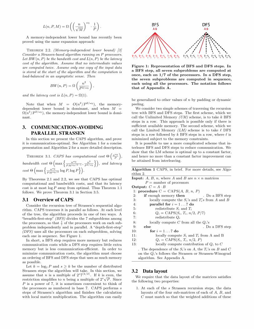
3.1 Overview of CAPSConsider the recursion tree of Strassen’s sequential algo-

rithm. CAPS traverses it in parallel as follows. At each levelof the tree, the algorithm proceeds in one of two ways. A“breadth-first-step” (BFS) divides the 7 subproblems amongthe processors, so that 1

7of the processors work on each sub-

problem independently and in parallel. A “depth-first-step”(DFS) uses all the processors on each subproblem, solvingeach one in sequence. See Figure 1.

In short, a BFS step requires more memory but reducescommunication costs while a DFS step requires little extramemory but is less communication-efficient. In order tominimize communication costs, the algorithm must choosean ordering of BFS and DFS steps that uses as much memoryas possible.

Let k = log7 P and s ≥ k be the number of distributedStrassen steps the algorithm will take. In this section, weassume that n is a multiple of 2s7dk/2e. If k is even, therestriction simplifies to n being a multiple of 2s

√P . Since

P is a power of 7, it is sometimes convenient to think ofthe processors as numbered in base 7. CAPS performs ssteps of Strassen’s algorithm and finishes the calculationwith local matrix multiplication. The algorithm can easily

Figure 1: Representation of BFS and DFS steps. Ina BFS step, all seven subproblems are computed atonce, each on 1/7 of the processors. In a DFS step,the seven subproblems are computed in sequence,each using all the processors. The notation followsthat of Appendix A.

be generalized to other values of n by padding or dynamicpeeling.

We consider two simple schemes of traversing the recursiontree with BFS and DFS steps. The first scheme, which wecall the Unlimited Memory (UM) scheme, is to take k BFSsteps in a row. This approach is possible only if there issufficient available memory. The second scheme, which wecall the Limited Memory (LM) scheme is to take ` DFSsteps in a row followed by k BFS steps in a row, where ` isminimized subject to the memory constraints.

It is possible to use a more complicated scheme that in-terleave BFS and DFS steps to reduce communication. Weshow that the LM scheme is optimal up to a constant factor,and hence no more than a constant factor improvement canbe attained from interleaving.

Algorithm 1 CAPS, in brief. For more details, see Algo-rithm 2.Input: A, B, n, where A and B are n× n matrices

P = number of processorsOutput: C = A ·B1: procedure C = CAPS(A, B, n, P )2: if enough memory then . Do a BFS step3: locally compute the Si’s and T ′i s from A and B4: parallel for i = 1 . . . 7 do5: redistribute Si and Ti

6: Qi = CAPS(Si, Ti, n/2, P/7)7: redistribute Qi

8: locally compute C from all the Qi’s9: else . Do a DFS step

10: for i = 1 . . . 7 do11: locally compute Si and Ti from A and B12: Qi = CAPS(Si, Ti, n/2, P )13: locally compute contribution of Qi to C

. The dependence of the Si’s on A, the Ti’s on B and Con the Qi’s follows the Strassen or Strassen-Winogradalgorithm. See Appendix A.

3.2 Data layoutWe require that the data layout of the matrices satisfies

the following two properties:

1. At each of the s Strassen recursion steps, the datalayouts of the four sub-matrices of each of A, B, andC must match so that the weighted additions of these

sub-matrices can be performed locally. This techniquefollows [25] and allows communication-free DFS steps.

2. Each of these submatrices must be equally distributedamong the P processors for load balancing.

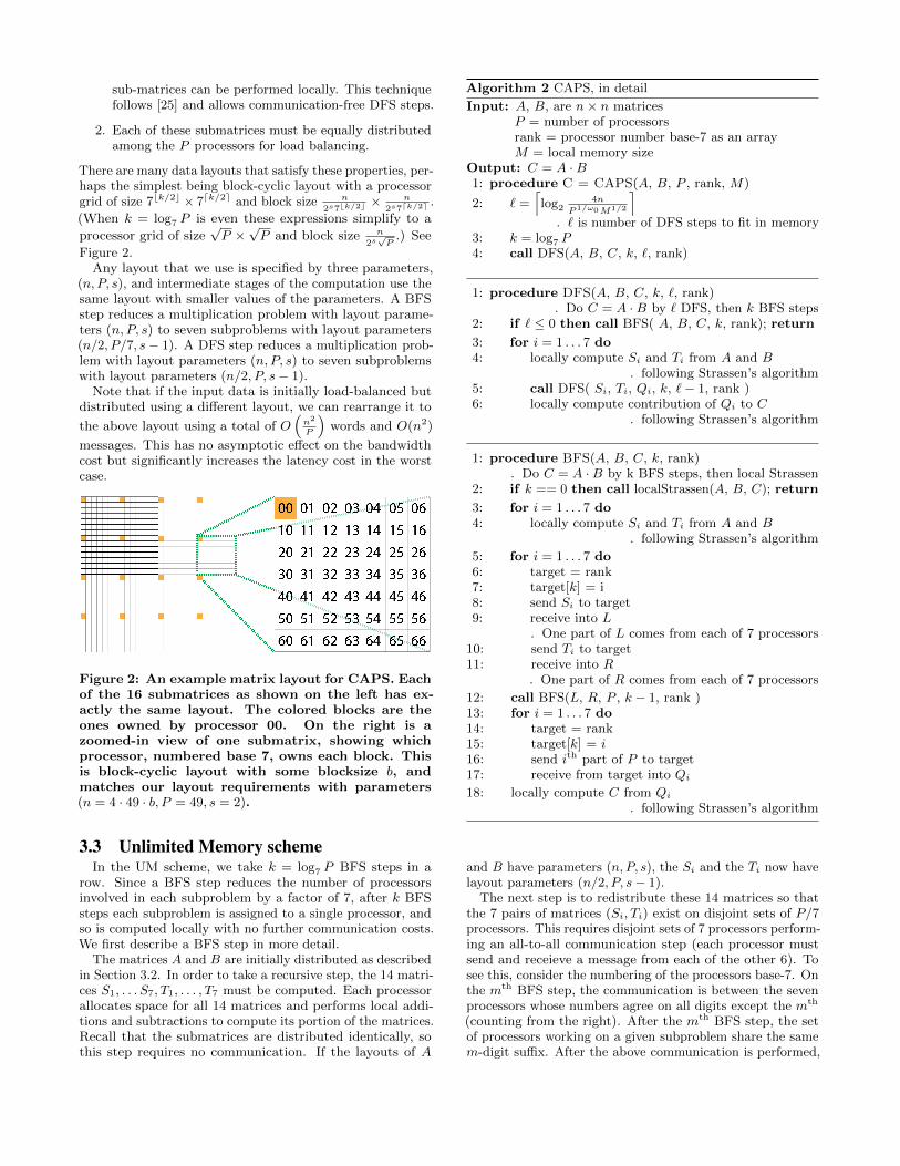
There are many data layouts that satisfy these properties, per-haps the simplest being block-cyclic layout with a processorgrid of size 7bk/2c × 7dk/2e and block size n

2s7bk/2c × n

2s7dk/2e .

(When k = log7 P is even these expressions simplify to a

processor grid of size√P ×

√P and block size n

2s√P

.) See

Figure 2.Any layout that we use is specified by three parameters,

(n, P, s), and intermediate stages of the computation use thesame layout with smaller values of the parameters. A BFSstep reduces a multiplication problem with layout parame-ters (n, P, s) to seven subproblems with layout parameters(n/2, P/7, s− 1). A DFS step reduces a multiplication prob-lem with layout parameters (n, P, s) to seven subproblemswith layout parameters (n/2, P, s− 1).

Note that if the input data is initially load-balanced butdistributed using a different layout, we can rearrange it to

the above layout using a total of O(

n2

P

)words and O(n2)

messages. This has no asymptotic effect on the bandwidthcost but significantly increases the latency cost in the worstcase.

Figure 2: An example matrix layout for CAPS. Eachof the 16 submatrices as shown on the left has ex-actly the same layout. The colored blocks are theones owned by processor 00. On the right is azoomed-in view of one submatrix, showing whichprocessor, numbered base 7, owns each block. Thisis block-cyclic layout with some blocksize b, andmatches our layout requirements with parameters(n = 4 · 49 · b, P = 49, s = 2).

3.3 Unlimited Memory schemeIn the UM scheme, we take k = log7 P BFS steps in a

row. Since a BFS step reduces the number of processorsinvolved in each subproblem by a factor of 7, after k BFSsteps each subproblem is assigned to a single processor, andso is computed locally with no further communication costs.We first describe a BFS step in more detail.

The matrices A and B are initially distributed as describedin Section 3.2. In order to take a recursive step, the 14 matri-ces S1, . . . S7, T1, . . . , T7 must be computed. Each processorallocates space for all 14 matrices and performs local addi-tions and subtractions to compute its portion of the matrices.Recall that the submatrices are distributed identically, sothis step requires no communication. If the layouts of A

Algorithm 2 CAPS, in detail

Input: A, B, are n× n matricesP = number of processorsrank = processor number base-7 as an arrayM = local memory size

Output: C = A ·B1: procedure C = CAPS(A, B, P , rank, M)

2: ` =⌈log2

4n

P1/ω0M1/2

⌉. ` is number of DFS steps to fit in memory

3: k = log7 P4: call DFS(A, B, C, k, `, rank)

1: procedure DFS(A, B, C, k, `, rank). Do C = A ·B by ` DFS, then k BFS steps

2: if ` ≤ 0 then call BFS( A, B, C, k, rank); return

3: for i = 1 . . . 7 do4: locally compute Si and Ti from A and B

. following Strassen’s algorithm5: call DFS( Si, Ti, Qi, k, `− 1, rank )6: locally compute contribution of Qi to C

. following Strassen’s algorithm

1: procedure BFS(A, B, C, k, rank). Do C = A ·B by k BFS steps, then local Strassen

2: if k == 0 then call localStrassen(A, B, C); return

3: for i = 1 . . . 7 do4: locally compute Si and Ti from A and B

. following Strassen’s algorithm

5: for i = 1 . . . 7 do6: target = rank7: target[k] = i8: send Si to target9: receive into L

. One part of L comes from each of 7 processors10: send Ti to target11: receive into R

. One part of R comes from each of 7 processors

12: call BFS(L, R, P , k − 1, rank )13: for i = 1 . . . 7 do14: target = rank15: target[k] = i16: send ith part of P to target17: receive from target into Qi

18: locally compute C from Qi

. following Strassen’s algorithm

and B have parameters (n, P, s), the Si and the Ti now havelayout parameters (n/2, P, s− 1).

The next step is to redistribute these 14 matrices so thatthe 7 pairs of matrices (Si, Ti) exist on disjoint sets of P/7processors. This requires disjoint sets of 7 processors perform-ing an all-to-all communication step (each processor mustsend and receieve a message from each of the other 6). Tosee this, consider the numbering of the processors base-7. Onthe mth BFS step, the communication is between the sevenprocessors whose numbers agree on all digits except the mth

(counting from the right). After the mth BFS step, the setof processors working on a given subproblem share the samem-digit suffix. After the above communication is performed,

the layout of Si and Ti has parameters (n/2, P/7, s− 1), andthe sets of processors that own the Ti and Si are disjointfor different values of i. Note that since each all-to-all onlyinvolves seven processors no matter how large P is, thisalgorithm does not have the scalability issues that typicallycome from an all-to-all communication pattern.

3.3.1 Memory requirementsThe extra memory required to take one BFS step is the

space to store all 7 triples Sj , Tj , Qj . Since each of thosematrices is 1

4the size of A, B, and C, the extra space

required at a given step is 7/4 the extra space required forthe previous step. We assume that no extra memory isrequired for the local multiplications.3 Thus, the total localmemory requirement for taking k BFS steps is given by

MemUM(n, P ) =3n2

P

k∑i=0

(7

4

)i

=7n2

P 2/ω0− 4n2

P

= Θ

(n2

P 2/ω0

).

3.3.2 Computation costsThe computation required at a given BFS step is that of the

local additions and subtractions associated with computingthe Si and Ti and updating the output matrix C with theQi. Since Strassen performs 18 additions and subtractions,the computational cost recurrence is

FUM(n, P ) = 18

(n2

4P

)+ FUM

(n

2,P

7

)with base case FUM(n, 1) = csn

ω0 − 6n2, where cs is theconstant of Strassen’s algorithm. See Appendix A for moredetails. The solution to this recurrence is

FUM(n, P ) =csn

ω0 − 6n2

P= Θ

(nω0

P

).

3.3.3 Communication costsConsider the communication costs associated with the

UM scheme. Given that the redistribution within a BFSstep is performed by an all-to-all communication step amongsets of 7 processors, each processor sends 6 messages andreceives 6 messages to redistribute S1, . . . , S7, and the samefor T1, . . . , T7. After the products Qi = SiTi are computed,each processor sends 6 messages and receive 6 messages toredistribute Q1, . . . , Q7. The size of each message variesaccording to the recursion depth, and is the number of words

a processor owns of any Si, Ti, or Qi, namely n2

4Pwords.

As each of the Qi is computed simultaneously on disjointsets of P/7 processors, we obtain a cost recurrence for theentire UM scheme:

BWUM(n, P ) = 36n2

4P+BWUM

(n

2,P

7

)LUM(n, P ) = 36 + LUM

(n

2,P

7

)3If one does not overwrite the input, it is impossible to runStrassen in place; however using a few temporary matricesaffects the analysis here by a constant factor only.

with base case LUM(n, 1) = BWUM(n, 1) = 0. Thus

BWUM(n, P ) =12n2

P 2/ω0− 12n2

P= Θ

(n2

P 2/ω0

)LUM(n, P ) = 36 log7 P = Θ (logP ) . (1)

3.4 Limited Memory schemeIn this section we discuss a scheme for traversing Strassen’s

recursion tree in the context of limited memory. In the LMscheme, we take ` DFS steps in a row followed by k BFSsteps in a row, where ` is minimized subject to the memoryconstraints. That is, we use a sequence of DFS steps toreduce the problem size so that we can use the UM schemeon each subproblem without exceeding the available memory.

Consider taking a single DFS step. Rather than allocatingspace for and computing all 14 matrices S1, T1, . . . , S7, T7 atonce, the DFS step requires allocation of only one subproblem,and each of the Qi will be computed in sequence.

Consider the ith subproblem: as before, both Si and Ti

can be computed locally. After Qi is computed, it is used toupdate the corresponding quadrants of C and then discardedso that its space in memory (as well as the space for Si andTi) can be re-used for the next subproblem. In a DFS step,no redistribution occurs. After Si and Ti are computed, allprocessors participate in the computation of Qi.

We assume that some extra memory is available. To beprecise, assume the matrices A, B, and C require only 1

3of

the available memory:

3n2

P≤ 1

3M. (2)

In the LM scheme, we set

` = max

0,

⌈log2

4n

P 1/ω0M1/2

⌉. (3)

The following subsection shows that this choice of ` issufficient not to exceed the memory capacity.

3.4.1 Memory requirementsThe extra memory requirement for a DFS step is the space

to store one subproblem. Thus, the extra space required atthis step is 1/4 the space required to store A, B, and C. Thelocal memory requirements for the LM scheme is given by

MemLM(n, P ) =3n2

P

`−1∑i=0

(1

4

)i

+ MemUM

( n2`, P)

≤ M

3

`−1∑i=0

(1

4

)i

+7(

n2`

)2P 2/ω0

≤ 127

144M < M,

where the last line follows from (3) and (2). Thus, the limitedmemory scheme does not exceed the available memory.

3.4.2 Computation costsAs in the UM case, the computation required at a given

DFS step is that of the local additions and subtractionsassociated with computing the Si and Ti and updating theoutput matrix C with the Qi. However, since all processorsparticipate in each subproblem and the subproblems are

computed in sequence, the recurrence is given by

FLM(n, P ) = 18

(n2

4P

)+ 7 · FLM

(n2, P).

After ` steps of DFS, the size of a subproblems is n2`× n

2`,

and there are P processors involved. We take k BFS stepsto compute each of these 7` subproblems. Thus

FLM

( n2`, P)

= FUM

( n2`, P),

and

FLM (n, P ) =18n2

4P

`−1∑i=0

(7

4

)i

+ 7` · FUM

( n2`, P)

=csn

ω0 − 6n2

P= Θ

(nω0

P

).

3.4.3 Communication costsSince there are no communication costs associated with a

DFS step, the recurrence is simply

BWLM(n, P ) = 7 ·BWLM

(n2, P)

LLM(n, P ) = 7 · LLM

(n2, P)

with base cases

BWLM

( n2`, P)

= BWUM

( n2`, P)

LLM

( n2`, P)

= LUM

( n2`, P).

Thus the total communication costs are given by

BWLM (n, P ) = 7` ·BWUM

( n2`, P)≤ 12 · 4ω0−2nω0

PMω0/2−1

= Θ

(nω0

PMω0/2−1

).

LLM (n, P ) = 7` · LUM

( n2`, P)≤ (4n)ω0

PMω0/236 log7 P

= Θ

(nω0

PMω0/2logP

). (4)

3.5 Communication optimalityProof. (of Theorem 3.1). In the case that M ≥

MemUM(n, P ) = Ω(

n2

P2/ω0

)the UM scheme is possible.

Then the communication costs are given by (1) which matchesthe lower bound of Theorem 2.2. Thus the UM scheme iscommunication-optimal (up to a logarithmic factor in the la-tency cost and assuming that the data is initially distributedas described in Section 3.2). For smaller values of M , theLM scheme must be used. Then the communication costsare given by (4) and match the lower bound of Theorem 2.1,so the LM scheme is also communication-optimal.

We note that for the LM scheme, since both the compu-tational and communication costs are proportional to 1

P,

we can expect perfect strong scaling: given a fixed problemsize, increasing the number of processors by some factorwill decrease each cost by the same factor. However, thisstrong scaling property has a limited range. As P increases,holding everything else constant, the global memory sizePM increases as well. The limit of perfect strong scaling isexactly when there is enough memory for the UM scheme.See [3] for details.

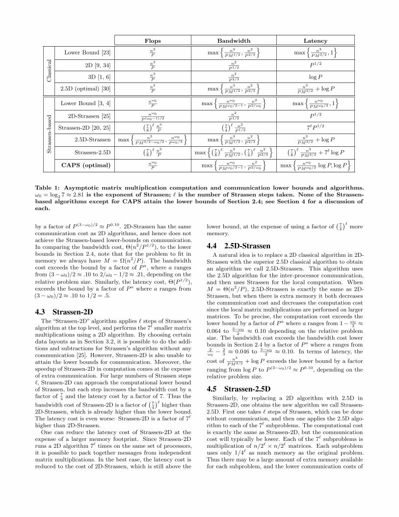
4. ANALYSIS OF OTHER ALGORITHMSIn the section we detail the asymptotic communication

costs of other matrix multiplication algorithms, both classicaland Strassen-based. These communication costs and thecorresponding lower bounds are summarized in Table 1.

Many of the algorithms described in this section are hybridsof two different algorithms. We use the convention that thenames of the hybrid algorithms are composed of the names ofthe two component algorithms, hyphenated. The first namedescribes the algorithm used at the top level, on the largestproblems, and the second describes the algorithm used atthe base level on smaller problems.

4.1 Classical AlgorithmsClassical algorithms must communicate asymptotically

more than an optimal Strassen-based algorithm. To comparethe lower bounds, it is necessary to consider three casesfor the memory size: when the memory-dependent boundsdominate for both classical and Strassen, when the memory-dependent bound dominates for classical, but the memory-independent bound dominates for Strassen, and when thememory-independent bounds dominate for both classical andStrassen. This analysis is detailed in Appendix B. Briefly,the factor by which the classical bandwidth cost exceedsthe Strassen bandwidth cost is P a where a ranges from2ω0− 2

3≈ 0.046 to 3−ω0

2≈ 0.10 depending on the relative

problem size. The same sort of analysis is used throughoutSection 4 to compare each algorithm with the Strassen-basedlower bounds.

Various parallel classical matrix multiplication algorithmsminimize communication relative to the classical lowerbounds for certain amounts of local memory M . For ex-ample, Cannon’s algorithm [9] minimizes communication forM = O(n2/P ). Several more practical algorithms exist (suchas SUMMA [34]) which use the same amount of local memoryand have the same asymptotic communication costs. Wecall this class of algorithms “2D” because the communicationpatterns follow a two-dimensional processor grid.

Another class of algorithms, known as “3D” [6, 1] becausethe communication pattern maps to a three-dimensionalprocessor grid, uses more local memory and reduces com-munication relative to 2D algorithms. This class of algo-rithms minimizes communication relative to the classicallower bounds for M = Ω(n2/P 2/3). As shown in [3], it is

not possible to use more memory than M = Θ(n2/P 2/3) toreduce communication.

Recently, a more general algorithm has been developedwhich minimizes communication in all cases. Because itreduces to a 2D and 3D for the extreme values of M butinterpolates for the values between, it is known as the “2.5D”algorithm [30].

4.2 2D-StrassenOne idea to parallelize Strassen-based algorithms is to

use a 2D classical algorithm for the inter-processor commu-nication, and use the fast matrix multiplication algorithmlocally [25]. We call such an algorithm “2D-Strassen”. 2D-Strassen is straightforward to implement, but cannot attainall the computational speedup from Strassen since it usesa classical algorithm for part of the computation. In par-ticular, it does not use Strassen for the largest matrices,when Strassen provides the greatest reduction in computa-tion. As a result, the computational cost exceeds Θ(nω0/P )

Flops Bandwidth Latency

Cla

ssic

al

Lower Bound [23] n3

Pmax

n3

PM1/2 ,n2

P2/3

max

n3

PM3/2 , 1

2D [9, 34] n3

Pn2

P1/2 P 1/2

3D [1, 6] n3

Pn2

P2/3 logP

2.5D (optimal) [30] n3

Pmax

n3

PM1/2 ,n2

P2/3

n3

PM3/2 + logP

Str

ass

en-b

ase

d

Lower Bound [3, 4] nω0

Pmax

nω0

PMω0/2−1 ,n2

P2/ω0

max

nω0

PMω0/2 , 1

2D-Strassen [25] nω0

P (ω0−1)/2n2

P1/2 P 1/2

Strassen-2D [20, 25](78

)` n3

P

(74

)` n2

P1/2 7`P 1/2

2.5D-Strassen max

n3

PM3/2−ω0/2 ,nω0

Pω0/3

max

n3

PM1/2 ,n2

P2/3

n3

PM3/2 + logP

Strassen-2.5D(78

)` n3

Pmax

(78

)` n3

PM1/2 ,(74

)` n2

P2/3

(78

)` n3

PM3/2 + 7` logP

CAPS (optimal) nω0

Pmax

nω0

PMω0/2−1 ,n2

P2/ω0

max

nω0

PMω0/2 logP, logP

Table 1: Asymptotic matrix multiplication computation and communication lower bounds and algorithms.ω0 = log2 7 ≈ 2.81 is the exponent of Strassen; ` is the number of Strassen steps taken. None of the Strassen-based algorithms except for CAPS attain the lower bounds of Section 2.4; see Section 4 for a discussion ofeach.

by a factor of P (3−ω0)/2 ≈ P 0.10. 2D-Strassen has the samecommunication cost as 2D algorithms, and hence does notachieve the Strassen-based lower-bounds on communication.In comparing the bandwidth cost, Θ(n2/P 1/2), to the lowerbounds in Section 2.4, note that for the problem to fit inmemory we always have M = Ω(n2/P ). The bandwidthcost exceeds the bound by a factor of P a, where a rangesfrom (3−ω0)/2 ≈ .10 to 2/ω0 − 1/2 ≈ .21, depending on the

relative problem size. Similarly, the latency cost, Θ(P 1/2),exceeds the bound by a factor of P a where a ranges from(3− ω0)/2 ≈ .10 to 1/2 = .5.

4.3 Strassen-2DThe “Strassen-2D” algorithm applies ` steps of Strassen’s

algorithm at the top level, and performs the 7` smaller matrixmultiplications using a 2D algorithm. By choosing certaindata layouts as in Section 3.2, it is possible to do the addi-tions and subtractions for Strassen’s algorithm without anycommunication [25]. However, Strassen-2D is also unable toattain the lower bounds for communication. Moreover, thespeedup of Strassen-2D in computation comes at the expenseof extra communication. For large numbers of Strassen steps`, Strassen-2D can approach the computational lower boundof Strassen, but each step increases the bandwidth cost by afactor of 7

4and the latency cost by a factor of 7. Thus the

bandwidth cost of Strassen-2D is a factor of(74

)`higher than

2D-Strassen, which is already higher than the lower bound.The latency cost is even worse: Strassen-2D is a factor of 7`

higher than 2D-Strassen.One can reduce the latency cost of Strassen-2D at the

expense of a larger memory footprint. Since Strassen-2Druns a 2D algorithm 7` times on the same set of processors,it is possible to pack together messages from independentmatrix multiplications. In the best case, the latency cost isreduced to the cost of 2D-Strassen, which is still above the

lower bound, at the expense of using a factor of(74

)`more

memory.

4.4 2.5D-StrassenA natural idea is to replace a 2D classical algorithm in 2D-

Strassen with the superior 2.5D classical algorithm to obtainan algorithm we call 2.5D-Strassen. This algorithm usesthe 2.5D algorithm for the inter-processor communication,and then uses Strassen for the local computation. WhenM = Θ(n2/P ), 2.5D-Strassen is exactly the same as 2D-Strassen, but when there is extra memory it both decreasesthe communication cost and decreases the computation costsince the local matrix multiplications are performed on largermatrices. To be precise, the computation cost exceeds thelower bound by a factor of P a where a ranges from 1− ω0

3≈

0.064 to 3−ω02≈ 0.10 depending on the relative problem

size. The bandwidth cost exceeds the bandwidth cost lowerbounds in Section 2.4 by a factor of P a where a ranges from2ω0− 2

3≈ 0.046 to 3−ω0

2≈ 0.10. In terms of latency, the

cost of n3

PM3/2 + logP exceeds the lower bound by a factor

ranging from logP to P (3−ω0)/2 ≈ P 0.10, depending on therelative problem size.

4.5 Strassen-2.5DSimilarly, by replacing a 2D algorithm with 2.5D in

Strassen-2D, one obtains the new algorithm we call Strassen-2.5D. First one takes ` steps of Strassen, which can be donewithout communication, and then one applies the 2.5D algo-rithm to each of the 7` subproblems. The computational costis exactly the same as Strassen-2D, but the communicationcost will typically be lower. Each of the 7` subproblems ismultiplication of n/2` × n/2` matrices. Each subproblemuses only 1/4` as much memory as the original problem.Thus there may be a large amount of extra memory availablefor each subproblem, and the lower communication costs of

the 2.5D algorithm help. The choice of ` that minimizes thebandwidth cost is

`opt = max

0,⌈log2

n

M1/2P 1/3

⌉.

The same choice minimizes the latency cost. Note that

when M ≥ n2

P2/3 , taking zero Strassen steps is optimal withrespect to communication. With ` = `opt, the bandwidthcost is a factor of P 1−ω0/3 ≈ P 0.064 above the lower boundsof Section 2.4. Additionally, the computation cost is notoptimal, and using ` = `opt, the computation cost exceeds theoptimal by a factor of P 1−ω0/3M3/2−ω0/2 ≈ P 0.064M0.096.

It is also possible to take ` > `opt steps of Strassen todecrease the comptutation cost further. However the de-creased computation cost comes at the expense of highercommunication cost, as in the case of Strassen-2D. In partic-ular, each extra step over `opt increases the bandwidth costby a factor of 7

4and the latency cost by a factor of 7. As

with Strassen-2D, it is possible to use extra memory to packtogether messages from several subproblems and decreasethe latency cost, but not the bandwidth cost.

5. PERFORMANCE RESULTSWe have implemented CAPS using MPI on a Cray XT4,

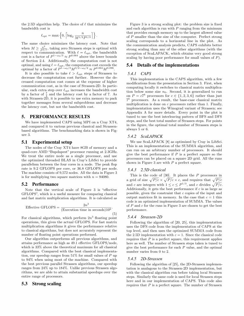
and compared it to various previous classical and Strassen-based algorithms. The benchmarking data is shown in Fig-ure 3.

5.1 Experimental setupThe nodes of the Cray XT4 have 8GB of memory and a

quad-core AMD “Bupdapest” processor running at 2.3GHz.We treat the entire node as a single processor, and usethe optimized threaded BLAS in Cray’s LibSci to provideparallelism between the four cores in a node. The peak floprate is 9.2 GFLOPS per core, or 36.8 GFLOPS per node.The machine consists of 9,572 nodes. All the data in Figure 3is for multiplying two square matrices with n = 94080.

5.2 PerformanceNote that the vertical scale of Figure 3 is “effective

GFLOPS”, which is a useful measure for comparing classicaland fast matrix multiplication algorithms. It is calculated as

Effective GFLOPS =2n3

(Execution time in seconds)109.

(5)For classical algorithms, which perform 2n3 floating pointoperations, this gives the actual GFLOPS. For fast matrixmultiplication algorithms it gives the performance relativeto classical algorithms, but does not accurately represent thenumber of floating point operations performed.

Our algorithm outperforms all previous algorithms, andattains performance as high as 49.1 effective GFLOPS/node,which is 33% above the theoretical maximum for all classicalalgorithms. Compared with the best classical implementa-tion, our speedup ranges from 51% for small values of P upto 94% when using most of the machine. Compared withthe best previous parallel Strassen algorithms, our speedupranges from 24% up to 184%. Unlike previous Strassen algo-rithms, we are able to attain substantial speedups over theentire range of processors.

5.3 Strong scaling

Figure 3 is a strong scaling plot: the problem size is fixedand each algorithm is run with P ranging from the minimumthat provides enough memory up to the largest allowed valueof P smaller than the size of the computer. Perfect strongscaling corresponds to a horizontal line in the plot. Asthe communication analysis predicts, CAPS exhibits betterstrong scaling than any of the other algorithms (with theexception of ScaLAPACK, which obtains very good strongscaling by having poor performance for small values of P ).

5.4 Details of the implementations

5.4.1 CAPSThis implementation is the CAPS algorithm, with a few

modifications from the presentation in Section 3. First, whencomputing locally it switches to classical matrix multiplica-tion below some size n0. Second, it is generalized to runon P = c7k processors for c ∈ 1, 2, 3, 6 rather than just7k processors. As a result, the base-case classical matrixmultiplication is done on c processors rather than 1. Finally,implementation uses the Winograd variant of Strassen; seeAppendix A for more details. Every point in the plot istuned to use the best interleaving pattern of BFS and DFSsteps, and the best total number of Strassen steps. For pointsin the figure, the optimal total number of Strassen steps isalways 5 or 6.

5.4.2 ScaLAPACKWe use ScaLAPACK [8] as optimized by Cray in LibSci.

This is an implementation of the SUMMA algorithm, andcan run on an arbitrary number of processors. It shouldgive the best performance if P is a perfect square so theprocessors can be placed on a square 2D grid. All the runsshown in Figure 3 are with P a perfect square.

5.4.3 2.5D classicalThis is the code of [30]. It places the P processors in

a grid of size√P/c ×

√P/c × c, and requires that

√P/c

and c are integers with 1 ≤ c ≤ P 1/3, and c divides√P/c.

Additionally, it gets the best performance if c is as large aspossible, given the constraint that c copies of the input andoutput matrices fit in memory. In the case that c = 1 thiscode is an optimized implementation of SUMMA. The valuesof P and c for the runs in Figure 3 are chosen to get the bestperformance.

5.4.4 Strassen-2DFollowing the algorithm of [20, 25], this implementation

uses the DFS code from the implementation of CAPS at thetop level, and then uses the optimized SUMMA code fromthe 2.5D implementation with c = 1. Since the classical coderequires that P is a perfect square, this requirement applieshere as well. The number of Strassen steps taken is tuned togive the best performance for each P value, and the optimalnumber varies from 0 to 2.

5.4.5 2D-StrassenFollowing the algorithm of [25], the 2D-Strassen implemen-

tation is analagous to the Strassen-2D implementation, butwith the classical algorithm run before taking local Strassensteps. Similarly the same code is used for local Strassen stepshere and in our implementation of CAPS. This code alsorequires that P is a perfect square. The number of Strassen

0

10

20

30

40

50

P=49 P=343 P=2401

Effe

ctive

GFL

OPS

per

nod

e absolute maximum for all classical algorithms

CAPS2.5D-Strassen

2D-StrassenStrassen-2D

2.5D ClassicalScaLAPACK

Figure 3: Strong scaling performance of various matrix multiplication algorithms on Cray XT4 for fixedproblem size n = 94080. The top line is CAPS as described in Section 3, and substantially outperforms all theother classical and Strassen-based algorithms. The horizontal axis is the number of nodes in log-scale. Thevertical axis is effective GFLOPS, which are a performance measure rather than a flop rate, as discussed inSection 5.2. See Section 5.4 for a description of each implementation.

steps is tuned for each P value, and the optimal numbervaries from 0 to 3.

5.4.6 2.5D-StrassenThis implementation uses the 2.5D implementation to

reduce the problem to one processor, then takes severalStrassen steps. The processor requirements are the sameas for the 2.5D implementation. The number of Strassensteps is tuned for each number of processors, and the optimalnumber varies from 0 to 3. We also tested the Strassen-2.5D algorithm, but its performance was always lower than2.5D-Strassen in our experiments.

6. CONCLUSIONS/FUTURE WORK

6.1 Stability of fast matrix multiplicationCAPS has the same stability properties as sequential ver-

sions of Strassen. For a complete discussion of the stabil-ity of fast matrix multiplication algorithms, see [21, 16].We highlight a few main points here. The tightest errorbounds for classical matrix multiplication are component-wise: |C−C| ≤ nε|A|·|B|, where C is the computed result andε is the machine precision. Strassen and other fast algorithms

do not satisfy component-wise bounds but do satisfy theslightly weaker norm-wise bounds: ‖C− C‖ ≤ f(n)ε‖A‖‖B‖,where ‖A‖ = maxi,j aij and f is polynomial in n [21]. Ac-curacy can be improved with the use of diagonal scalingmatrices: D1CD3 = D1AD2 · D−1

2 BD3. It is possible tochoose D1,D2,D3 so that the error bounds satisfy either|C−C| ≤ f(n)ε‖A(i, :)‖‖B(:, j)‖ or ‖C−C‖ ≤ f(n)ε‖|A|·|B|‖.By scaling, the error bounds on Strassen become comparableto those of many other dense linear algebra algorithms, suchas LU and QR decomposition [15]. Thus using Strassen forthe matrix multiplications in a larger computation will oftennot harm the stability at all.

6.2 Hardware scalingAlthough Strassen performs asymptotically less compu-

tation and communication than classical matrix multipli-cation, it is more demanding on the hardware. That is, ifone wants to run matrix multiplication near the peak CPUspeed, Strassen is more demanding of the memory size andcommunication bandwidth. This is because the ratio ofcomputational cost to bandwidth cost is lower for Strassenthan for classical. From the lower bounds in Section 2.4, theasymptotic ratio of computational cost to bandwidth cost

is Mω0/2−1 for Strassen-based algorithms, versus M1/2 forclassical algorithms. This means that it is harder to runStrassen near peak than it is to run classical matrix multipli-cation near peak. In terms of the machine parameters β andγ introduced in Section 2.1, the condition to be able to becompute-bound is γM1/2 ≥ cβ for classical matrix multipli-cation and γMω0/2−1 ≥ c′β for Strassen. Here c and c′ areconstants that depend on the constants in the communica-tion and computational costs of classical and Strassen-basedmatrix multiplication.

The above inequalities may guide hardware design as longas classical and Strassen matrix multiplication are consideredimportant computations. They apply both to the distributedcase, where M is the local memory size and β is the inversenetwork bandwidth, and to the sequential/shared-memorycase where M is the cache size and β is the inverse memory-cache bandwidth.

6.3 Optimizing on-node performanceNote that although our implementation performs above

the classical peak performance, it performs well below thecorresponding Strassen-Winograd peak, defined by the timeit takes to perform csn

ω0/P flops at the peak speed of eachprocessor. To some extent, this is because Strassen is moredemanding on the hardware, as noted above. However wehave not yet analyzed whether the amount our performanceis below Strassen peak can be entirely accounted for basedon machine parameters. It is also possible that a high per-formance shared memory Strassen implementation mightprovide substantial speedups for our implementation.

6.4 Testing on various architecturesWe have implemented and benchmarked CAPS on only

one architecture, a Cray XT4. It remains to check thatit outperforms other matrix multiplication algorithms on avariety of architectures. On some architectures it may bemore important to consider the topology of the network andredesign the algorithm to minimize contention, which wehave not done.

6.5 Improvements to the algorithmTo be practically useful, it is important to generalize the

number of processors on which CAPS can run. To attainthe communication lower bounds, CAPS as presented inSection 3 must run on P a power of seven processors. Ofcourse, CAPS can then be run on any number of processorsby simply ignoring no more than 6

7of them and incurring

a constant factor overhead. Thus we can run on arbitraryP and attain the communication and computation lowerbounds up to a constant factor. However the computationtime is still dominant in most cases, and it is preferableto attain the computation lower bound exactly. It is anopen question whether any algorithm can run on arbitraryP , attain the computation lower bound exactly, and attainthe communication lower bound up to a constant factor.

Moreover, although the communication costs of this al-gorithm match the lower bound up to a constant factor inbandwidth, and up to a logP factor in latency, it is anopen question to determine the optimal constant in the lowerbound and perhaps provide a new algorithm that matches itexactly. Note that in the analysis of CAPS in Section 3, theconstants could be slightly improved.

6.6 Parallelizing other recursive algorithms

6.6.1 Other fast matrix multiplication algorithmsOur approach of executing a recursive algorithm in parallel

by traversing the recursion tree in DFS (sequential) or BFS(parallel) manners is not limited to Strassen’s algorithm. Allfast matrix multiplication algorithms are built out of waysto multiply a m×n matrix by a n× k matrix using q < mnkmultiplications. Like with Strassen and Strassen-Winograd,they compute q linear combinations of entries of each of Aand B, multiply these pairwise, then compute the entriesof C as linear combinations of these.4 CAPS can be easilygeneralized to any such multiplication, with the followingmodifications:

• The number of processors P is a power of q.

• The data layout must be such that all m× n blocks ofA, all n× k blocks of B, and all m× k blocks of C aredistributed equally among the P processors with thesame layout.

• The BFS and DFS determine whether the q multipli-cations are performed in parallel or sequentially.

The communication costs are then exactly as above, but withω0 = 3 logmnk q.

It is unclear whether any of the faster matrix multiplica-tion algorithms are useful in practice. One reason is thatthe fastest algorithms are not explicit. Rather, there arenon-constructive proofs that the algorithms exist. To imple-ment these algorithms, they would have to be found, whichappears to be a difficult problem. The generalization ofCAPS described in this section does apply to all of them, sowe have proved the existence of a communication-avoidingnon-explicit parallel algorithm corresponding to every fastmatrix multiplication algorithm. We conjecture that the al-gorithms are all communication-optimal, but that is not yetproved since the lower bound proofs in [4, 3] may not applyto all fast matrix multiplication algorithms. In cases wherethe lower bounds do apply, they match the performance ofthe generalization of CAPS, and so they are communication-optimal.

6.6.2 Another communication-optimal classicalalgorithm

We can apply our parallelization approach to recursiveclassical matrix multiplication to obtain a communication-optimal algorithm. This algorithm has the same asymptoticcommunication costs as the 2.5D algorithm [30], althoughthe constants in its communication costs are higher. Weobserved comparable performance to the 2.5D algorithm onour experimental platform. As with CAPS, this algorithmhas not been optimized for contention, whereas the 2.5Dalgorithm is very well optimized for contention on torusnetworks.

7. REFERENCES[1] R. C. Agarwal, S. M. Balle, F. G. Gustavson, M. Joshi,

and P. Palkar. A three-dimensional approach to parallelmatrix multiplication. IBM Journal of Research andDevelopment, 39:39–5, 1995.

4By [27], all fast matrix multiplication algorithms can beexpressed in this bilinear form.

[2] A. Aggarwal, A. K. Chandra, and M. Snir.Communication complexity of PRAMs. Theor. Comput.Sci., 71:3–28, March 1990.

[3] G. Ballard, J. Demmel, O. Holtz, B. Lipshitz, andO. Schwartz. Strong scaling of matrix multiplicationalgorithms and memory-independent communicationlower bounds, 2012. Manuscript, submitted to SPAA2012.

[4] G. Ballard, J. Demmel, O. Holtz, and O. Schwartz.Graph expansion and communication costs of fastmatrix multiplication. In SPAA ’11: Proceedings of the23rd annual symposium on parallelism in algorithmsand architectures, pages 1–12, New York, NY, USA,2011. ACM.

[5] G. Ballard, J. Demmel, O. Holtz, and O. Schwartz.Minimizing communication in numerical linear algebra.SIAM J. Matrix Analysis Applications, 32(3):866–901,2011.

[6] J. Berntsen. Communication efficient matrixmultiplication on hypercubes. Parallel Computing,12(3):335 – 342, 1989.

[7] D. Bini. Relations between exact and approximatebilinear algorithms. applications. Calcolo, 17:87–97,1980. 10.1007/BF02575865.

[8] L. S. Blackford, J. Choi, A. Cleary, E. DSAzevedo,J. Demmel, I. Dhillon, J. Dongarra, S. Hammarling,G. Henry, A. Petitet, K. Stanley, D. Walker, and R. C.Whaley. ScaLAPACK Users’ Guide. SIAM,Philadelphia, PA, USA, May 1997. Also available fromhttp://www.netlib.org/scalapack/.

[9] L. Cannon. A cellular computer to implement theKalman filter algorithm. PhD thesis, Montana StateUniversity, Bozeman, MN, 1969.

[10] J. Choi. A new parallel matrix multiplication algorithmon distributed-memory concurrent computers.Concurrency: Practice and Experience, 10(8):655–670,1998.

[11] J. Choi, D. W. Walker, and J. J. Dongarra. PUMMA:Parallel universal matrix multiplication algorithms ondistributed memory concurrent computers.Concurrency: Practice and Experience, 6(7):543–570,1994.

[12] H. Cohn, R. D. Kleinberg, B. Szegedy, and C. Umans.Group-theoretic algorithms for matrix multiplication.In FOCS, pages 379–388, 2005.

[13] D. Coppersmith and S. Winograd. On the asymptoticcomplexity of matrix multiplication. SIAM Journal onComputing, 11(3):472–492, 1982.

[14] D. Coppersmith and S. Winograd. Matrixmultiplication via arithmetic progressions. InProceedings of the Nineteenth Annual ACM Symposiumon Theory of Computing, STOC ’87, pages 1–6, NewYork, NY, USA, 1987. ACM.

[15] J. Demmel, I. Dumitriu, and O. Holtz. Fast linearalgebra is stable. Numerische Mathematik,108(1):59–91, 2007.

[16] J. Demmel, I. Dumitriu, O. Holtz, and R. Kleinberg.Fast matrix multiplication is stable. NumerischeMathematik, 106(2):199–224, 2007.

[17] F. Desprez and F. Suter. Impact of mixed-parallelismon parallel implementations of the Strassen andWinograd matrix multiplication algorithms: Research

articles. Concurr. Comput. : Pract. Exper., 16:771–797,July 2004.

[18] S. H. Fuller and L. I. Millett, editors. The Future ofComputing Performance: Game Over or Next Level?The National Academies Press, Washington, D.C.,2011. 200 pages, http://www.nap.edu.

[19] S. L. Graham, M. Snir, and C. A. Patterson, editors.Getting up to Speed: The Future of Supercomputing.Report of National Research Council of the NationalAcademies Sciences. The National Academies Press,Washington, D.C., 2004. 289 pages,http://www.nap.edu.

[20] B. Grayson, A. Shah, and R. van de Geijn. A highperformance parallel Strassen implementation. InParallel Processing Letters, volume 6, pages 3–12, 1995.

[21] N. J. Higham. Accuracy and Stability of NumericalAlgorithms. SIAM, Philadelphia, PA, 2nd edition, 2002.

[22] S. Hunold, T. Rauber, and G. Runger. Combiningbuilding blocks for parallel multi-level matrixmultiplication. Parallel Computing, 34:411–426, July2008.

[23] D. Irony, S. Toledo, and A. Tiskin. Communicationlower bounds for distributed-memory matrixmultiplication. J. Parallel Distrib. Comput.,64(9):1017–1026, 2004.

[24] B. Kumar, C.-H. Huang, R. Johnson, andP. Sadayappan. A tensor product formulation ofStrassen’s matrix multiplication algorithm withmemory reduction. In Proceedings of SeventhInternational Parallel Processing Symposium, pages 582–588, apr 1993.

[25] Q. Luo and J. Drake. A scalable parallel Strassen’smatrix multiplication algorithm for distributed-memorycomputers. In Proceedings of the 1995 ACM symposiumon Applied computing, SAC ’95, pages 221–226, NewYork, NY, USA, 1995. ACM.

[26] V. Y. Pan. New fast algorithms for matrix operations.SIAM Journal on Computing, 9(2):321–342, 1980.

[27] R. Raz. On the complexity of matrix product. SIAM J.Comput., 32(5):1356–1369 (electronic), 2003.

[28] F. Romani. Some properties of disjoint sums of tensorsrelated to matrix multiplication. SIAM Journal onComputing, 11(2):263–267, 1982.

[29] A. Schonhage. Partial and total matrix multiplication.SIAM Journal on Computing, 10(3):434–455, 1981.

[30] E. Solomonik and J. Demmel. Communication-optimalparallel 2.5D matrix multiplication and LUfactorization algorithms. In Euro-Par’11: Proceedingsof the 17th International European Conference onParallel and Distributed Computing. Springer, 2011.

[31] F. Song, J. Dongarra, and S. Moore. Experiments withStrassen’s algorithm: From sequential to parallel. InProceedings of Parallel and Distributed Computing andSystems (PDCS). ACTA, Nov. 2006.

[32] V. Strassen. Gaussian elimination is not optimal.Numer. Math., 13:354–356, 1969.

[33] V. Strassen. Relative bilinear complexity and matrixmultiplication. Journal fur die reine und angewandteMathematik (Crelles Journal), 1987(375–376):406–443,1987.

[34] R. A. van de Geijn and J. Watts. SUMMA: scalable

universal matrix multiplication algorithm. Concurrency- Practice and Experience, 9(4):255–274, 1997.

[35] V. V. Williams. Breaking the Coppersmith-Winogradbarrier, 2012. Manuscript.

[36] S. Winograd. On the multiplication of 2 × 2 matrices.Linear Algebra Appl., 4(4):381–388., October 1971.

[37] C.-Q. Yang and B. Miller. Critical path analysis for theexecution of parallel and distributed programs. InProceedings of the 8th International Conference onDistributed Computing Systems, pages 366–373, Jun.1988.

APPENDIXA. STRASSEN-WINOGRAD ALGORITHM

The Strassen-Winograd algorithm is usually preferred toStrassen’s algorithm in practice since it requires fewer addi-tions. We use it for our implementation of CAPS. Divide theinput matrices A,B and output matrix C into 4 submatrices:

A =

[A11 A12

A21 A22

]B =

[B11 B12

B21 B22

]C =

[C11 C12

C21 C22

]

Then form 7 linear combinations of the submatrices of eachof A and B, call these Ti and Si, respectively; multiplythem pairwise; then form the submatrices of C as linearcombinations of these products:

T0 = A11 S0 = B11 Q0 = T0 · S0 U1 = Q0 + Q3

T1 = A12 S1 = B21 Q1 = T1 · S1 U2 = U1 + Q4

T2 = A21 + A22 S2 = B12 + B11 Q2 = T2 · S2 U3 = U1 + Q2

T3 = T2 − A12 S3 = B22 − S2 Q3 = T3 · S3 C11 = Q0 + Q1

T4 = A11 − A21 S4 = B22 − B12 Q4 = T4 · S4 C12 = U3 + Q5

T5 = A12 + T3 S5 = B22 Q5 = T5 · S5 C21 = U2 − Q6

T6 = A22 S6 = S3 − B21 Q6 = T6 · S6 C22 = U2 + Q2

This is one step of Strassen-Winograd. The algorithmis recursive since it can be used for each of the 7 smallermatrix multiplications. In practice, one often uses only afew steps of Strassen-Winograd, although to attain O(nω0)computational cost, it is necessary to recursively apply it allthe way down to matrices of size O(1)×O(1). The precisecomputational cost of Strassen-Winograd is

F(n) = csnω0 − 5n2.

Here cs is a constant depending on the cutoff point at whichone switches to the classical algorithm. For a cutoff size ofn0, the constant is cs = (2n0 + 4)/nω0−2

0 which is minimizedat n0 = 8 yielding a computational cost of approximately3.73nω0−5n2. If using Strassen-Winograd with cutoff n0 thisshould be substituted into the computational cost expressionsof Section 3.

B. COMMUNICATION-COST RATIOSIn this section we derive the ratio R of classical to Strassen-

based bandwidth cost lower bounds that appear in the begin-ning of Section 4. Note that both classical and Strassen-basedlower bounds are attained by optimal algorithms. Similarderivations apply to the other ratios quoted in that section.Because the bandwidth cost lower bounds are different inthe memory-dependent and the memory-independent cases,and the threshold between these is different for the classicaland Strassen-based bounds, it is necessary to consider threecases.

Case 1. M = Ω(n2/P ) and M = O(n2/P 2/ω0). The firstcondition is necessary for there to be enough memory tohold the input and output matrices; the second conditionputs both classical and Strassen-based algorithms in thememory-dependent case. Then the ratio of the bandwidthcosts is:

R = Θ

(n3

PM1/2

/nω0

PMω0/2−1

)= Θ

((n2

M

)(3−ω0)/2).

Using the two bounds that define this case, we obtain R =O(P (3−ω0)/2) and R = Ω(P 3/ω0−1).

Case 2. M = Ω(n2/P 2/ω0) and M = O(n2/P 2/3). Thismeans that in the classical case the memory-dependent lowerbound dominates, but in the Strassen-based case the memory-independent lower bound dominates. Then the ratio is:

R = Θ

(n3

PM1/2

/n2

P 2/ω0

)= Θ

((n2

M

)1/2

P 2/ω0−1

).

Using the two bounds that define this case, we obtain R =O(P 3/ω0−1) and R = Ω(P 2/ω0−2/3).

Case 3. M = O(P 2/3). This means that both the classi-cal and Strassen-based lower bounds are dominated by thememory-independent cases. Then the ratio is:

R = Θ

(n2

P 2/3

/n2

P 2/ω0

)= Θ

(P 2/ω0−2/3

).

Overall, depending on the ratio of the problem size to theavailable memory, the factor by which the classical bandwidthcosts exceed the Strassen-based bandwidth costs is betweenΘ(P 2/ω0−2/3) and Θ(P (3−ω0)/2).