Communication in Repeated Games with Costly

Monitoring

Elchanan Ben-Porath1 and Michael Kahneman

January, 2002

1The department of Economics and the Center for Rationality, the Hebrew University of

Jerusalem, and the Eitan Berglas School of Economics, Tel-Aviv University. Correspondence:

Elchanan Ben-Porath, the Center for Rationality, Feldman building, the Hebrew University, Givaat-

Ram, Jerusalem, Israel. e-mail: benporat@math.huji.ac.il Fax: 972-2-6513681.

Abstract

We study repeated games with discounting where perfect monitoring is possible, but costly.

It is shown that if players can make public announcements, then every payoff vector which is

an interior point in the set of feasible and individually rational payoffs can be implemented

in a sequential equilibrium of the repeated game when the discount factor is high enough.

Thus, efficiency can be approximated even when the cost of monitoring is high, provided

that the discount factor is high enough.

Key words: Repeated games, costly monitoring, communication.

1

1 INTRODUCTION

The basic results in the theory of repeated games (Aumann and Shapley, 1976; Fudenburg

and Maskin, 1986, and Rubinstein, 1979) establish that every individual rational payoff,

(that is, a feasible payoff which is above the minmax point), is a perfect equilibrium payoff.

In particular, repetition can enable players to obtain efficient outcomes in equilibrium. An

important assumption that underlies these results is that each player can costlessly observe

the past actions of the other players. Here we assume that perfect monitoring is possible but

costly. It is shown that if players can make public announcements then, under a standard

assumption of full dimensionality of the payoff set, the limit set of sequential equilibrium

payoffs contains the set of individual rational payoffs. Thus, efficiency can be approximated

even when the cost of monitoring is high, provided that the discount factor is high enough.

In particular, as the discount factor tends to 1, monitoring can be more sparse so that the

average cost of monitoring per period tends to zero.

The setup is as follows: The starting point is an n-person one-shot game G. We now

consider an extension of G, G, in which each player i can observe the actions of some set of

players Q at a cost Ci(Q). Formally, we associate with each action ai for player i and any set

of players different from i, Q, an action (ai, Q).When (ai, Q) is played, player i observes the

actions that were played by members of Q and her payoff is her payoff in G minus the cost

of observation Ci(Q).1 The only assumption we make on Ci(Q) is that it is increasing, so if

Q0 ⊆ Q then Ci(Q0) ≤ Ci(Q).2 There are no restrictions on the costs of observing, so Ci(Q)can be any finite non-negative number. The game G is played repeatedly and we assume that

at the end of each period, players can make public announcements. The payoff in the repeated

game is a discounted sum of the one-shot payoffs. We are interested in the behavior of the set

1To obtain our result we only need to assume that player i can observe one other player at each period.2This assumption is in fact not necessary but it makes the exposition simpler.

2

V (G) which is the limit of the set of sequential equilibrium payoffs when the discount factor

tends to 1. The result is that V (G) contains the set of feasible and individually rational

payoffs of the original game G provided that the latter set is n−dimensional.To keep the exposition simple, we assume that player i observes only the action of

the members of Q and, of course, her own actions, but nothing else. However, our result

can be immediately extended to the case where each player can observe some public, or

even private, signal for free, provided that a standard assumption of common support is

satisfied.3 This extension is important because there are games of economic interest in the

literature which have this structure. One example is partnership games which have been

studied by Radner (1986) and Radner, Myerson and Maskin (1986). In these games, each

worker/partner chooses a level of effort and the profile of efforts determines a distribution

on the joint production. The joint production level is a public signal that is observed (for

free) by everyone. When low production is observed it is not clear if one of the players has

deviated or if it is just an unfortunate outcome. Radner, Myerson and Maskin provide an

example which demonstrates that this problem may cause equilibrium payoffs to be bounded

away from efficiency. Our result implies that if it is possible to observe the effort of a given

worker for some cost, (which can be arbitrarily high), then efficiency can be approximated

as the discount factor tends to 1.

Another celebrated example is repeated Cournot games with imperfect monitoring.

In these games the quantity that each firm produces is not observed. The only observable

parameter is the price of the product which is a stochastic function of the aggregate pro-

duction. Green and Porter (1984) and Abreu, Pearce and Stachetti (1986) have shown that

3A signal function is a stochastic function that associates with each profile of actions of the players a

probability distribution over a set of signals. The common support assumption is that all the probability

distributions that are associated with the different action profiles have the same support.

3

in symmetric games optimal equilibria have a simple structure and that efficiency cannot

be obtained. Again, our result implies that if monitoring is possible, then even if its cost is

high, efficiency can be approximated.

Most of the literature on games with imperfect monitoring has focused on games

with public signals.4 For example, in the partnership game the signal that each player

observes is the joint production level. In the Cournot game it is the price. In most real

interactions players observe private signals. For example, a real situation which exhibits the

problem modeled by the partnership game will almost surely have each worker observing

some private signal of the effort invested by other workers. The study of repeated games

with private monitoring has been relatively limited. Lehrer has studied two person games

where payoffs are evaluated by the limit of the means (Lehrer 1990, 1992a, and 1992b).

Fudenberg and Levine (1991) study N-person games with discounting but use an ²-sequential

equilibrium notion, which is a significantly weaker notion than sequential equilibrium. The

closest studies to the current one are Compte (1998) and Kandori and Matsushima (1998).

Kandori and Matsushima examine, as do we, the limit behavior of the set of sequential

equilibrium payoffs in a repeated game with discounting. They assume, as it is done here,

that players can make public announcements and that the signals that players observe have

a common support. They then provide two conditions on the signals which ensure that

every individual rational payoff belongs to the limit set of equilibrium payoffs. The first

condition is that if either player i or player j deviates, then the other players, putting their

information together, can statistically detect that. The second condition is that, given that

player i or player j have deviated, the other players, (putting their information together), can

statistically detect which one of them it was. Compte obtains a similar result using different

4General studies of such games can be found in Abreu, Pearce and Stachetti (1990), Fudenberg, Levine

and Maskin (1994), and Lehrer (1990b).

4

assumptions on the signals. Thus, the relationship of these two papers to the current study

is that the assumption of costly perfect monitoring is substituted by assumptions on the

informativeness of the signals.

The assumptions that underlie the basic Falk Theorem can be decomposed as follows:

(1) Each player can observe the action of every other player.

(2) Each observation is a perfect observation.

(3) Each observation is costless.

The current paper relaxes the third assumption.

In Ben-Porath and Kahneman (1996) we relaxed the first assumption and showed that

if each player can be observed by at least two other players then the limit set of sequential

equilibrium payoffs contains the set of individual rational payoffs5. In the equilibria that

we construct in the current paper we do not need to assume that a given player is observed

by more than two players. Since the construction here applies to the case where the cost of

monitoring is zero as well, the result in the current paper extends the result in the previous

paper for discounted games. Furthermore, in the equilibria that we construct here each

player is observed by just one other player in any given period. (However, in case of a

deviation the monitor of a given player i is substituted, so we do need at least two players

who have the ability to observe i.)

The equilibria that we will define are somewhat involved so it is worthwhile to list

the main ideas in the construction. We consider first the case of three or more players and

then comment on the case of two players. The first observation is that to obtain efficiency

monitoring, which is costly, should be sparse. This immediately implies that the monitoring

should be random and that the probability of being monitored in each particular period is

5In the first paper we also showed that if payoffs are evaluated by the lim inf of the means then it is

possible to cooperate even when each player can be monitored by only one other player.

5

low. Now, when the discount factor is close to one it is possible to inflict harsh punishments

and therefore it is possible to deter a player from deviating even when the probability of

detection is low. Next, we note that since the act of observing is costly and is itself unobserved

there is a need to provide incentives to do it. So if player j monitors player i in period t

then player j should be uncertain about the action of player i in period t. To deal with these

issues we propose an equilibrium which has the following general structure: Time is divided

into segments of K periods. Each player i has a player which monitors him, q(i). At the

beginning of a segment player q(i) chooses at random a period t1 in the segment in which

she will observe player i, and player i chooses at random a period t26 in which she ‘switches’

and plays an action which is different from the action that is specified by the main path.

At the end of the segment player i publicly announces the period t2 and her action in that

period and player q(i) announces the period t1 and her observation of the action of player i.

The two announcements are made simultaneously. If the announcements are incompatible

then one of the players has deviated. Conversely, if one of the players deviates - player q(i)

by guessing the action of player i rather than observing it, or player i by departing from

the main path more than once - then with a probability of at least 1K, (K is the number of

periods in a segment), there will be a mismatch in the announcements. Thus, the way to

deter players from deviating is to initiate a sufficiently severe punishment whenever there is a

mismatch in the announcements.7 Since it is impossible to tell which one of the two players,

6In fact player i chooses two periods but the reason for that is not important.7The idea of checking whether the player q(i) has monitored player i by having player i switch from the

main path is related to an idea which appears in Lehrer (1992a). Specifically, let ai and ai be two actions

for player i such that ai is less informative than ai, that is, there exist actions aj and aj for player j such

that if player i plays ai she can distinguish between aj and aj , (i.e., she gets a different signal in each case),

while if she plays ai she gets the same signal. In the equilibrium which Lehrer constructs a deviation from

ai to ai is deterred in the following way: Player j picks at random periods in which she randomizes between

aj and aj . Player i is then ”asked” to reveal his signals in these periods. If he gives a wrong answer he is

6

i or q(i), has deviated both of them are punished. The problem in punishing two players is

that in general it is impossible to punish the same pair of players (i, q(i)) repeatedly. So

if (i, q(i)) continue to make contradicting statements repeatedly there will be a period in

which it will not be possible to further decrease the payoffs of both of them. The reason

for this difficulty is that in general the minmax profile of actions for player i is different from

the minmax profile for player q(i) so it is impossible to minmax both players at the same

time. The way to deal with this problem is to change the monitoring assignment q( ) each

time that a mismatch of announcements occurs so that a new mismatch of announcements

will involve a pair of players that is different from the last pair that was punished. If, for

example, player i and her monitor k contradict each other, then the equilibrium moves to a

phase in which i and k are punished and the new monitoring assignment is such that i and

k do not monitor each other. So if there will be a new case of contradicting statements in

this punishment phase it will involve a pair of players different from (i, k). In this manner

the same pair of players is not punished twice in a row.

In the case of two players each player must monitor the other all along the game so

the construction has to be modified. The new feature here is that there are subgames in

which the harshness of the punishment that can be implemented is limited and therefore

there is a need to increase the density of the monitoring so that the probability of detection

in case of a deviation will be high enough.

At this point the reader might wonder why we chose theK−periods segment structurerather than work with simpler strategies in which each player i is monitored each period

with a small probability. The problem with these simpler strategies is that to have player

j randomize between monitoring and not monitoring player j has to be indifferent between

these two options which means that she has to be compensated in case she monitors. Now

punished.

7

the point is that if player j has to monitor player i in a long sequence of consecutive periods,

(such an event happens with a positive probability), then because of the discounting the

compensation that player j should receive in the subgame that follows is higher than what is

feasible.8 This problem of infeasible compensation does not arise in the equilibrium that we

have outlined because in this equilibrium the density of the monitoring is fixed (one period

every K periods).

The paper is organized as follows. The model and the results are presented in Section

2. In Section 3 we illustrate the main feature of the equilibria that we propose in the context

of a simple partnership game. Section 4 contains the proof of the result for the case where

the number of players is at least three. In Section 5 the case of two players is addressed.A

complete characterization of V (G) seems to be difficult to obtain and is beyond the scope of

this paper. However, in the concluding section, section 6, we make a few observations that

are related to this problem.

2 The Model and the Result

The component game G is defined as follows: Each player i, i ∈ N ≡ 1, ..., n, chooses anaction ai from a finite set of actions Ai. A profile of actions a, a ∈ A ≡ Πni=1Ai, determines

a payoff gi(a) for player i.

Let Σi denote the set of mixed actions for player i with a generic element αi. We let

gi(α), α ∈ Σ ≡ Πni=1 Σi, denote the expected payoff when α is played.

We assume that player i can perfectly observe the actions of a set of players Q, Q ⊆8Putting it a bit differently the problem is as follows: After a long sequence of consecutive periods in

which player j has monitored player i her payoff in the continuation of the game is so close to the maximal

payoff that is feasible that it will be impossible to compensate player j for the cost of monitoring in the next

period.

8

N − i for some cost Ci(Q), 0 <− Ci(Q) < ∞, where Ci(∅) = 0 and Ci(Q) ≥ Ci(Q0)

if Q ⊇ Q0. Formally, we extend the game by associating with each action ai 2n−1 actions(ai, Qi), Qi ⊆ N−i, so that when (a,Q) is played, (a,Q) = (aj, Qj)nj=1, player i learns theaction of each player inQi. Let G denote the extended game and let Ai, Σi, and gi denote,

respectively, the set of pure actions for player i, the set of mixed actions for player i, and

the expected payoff for player i. So,

Ai = Ai × 2N−i.

gi(a,Q) ≡ gi(a)− Ci(Qi).

The function gi9 is extended to the space of mixed actions in the obvious way.

Let:

Z ≡ maxi

maxa∈A,a0i∈Ai,Qi⊆N−i

gi(a0i, a−i)− gi(a,Qi).

Thus, Z is an upper bound on the benefit from a deviation in the extended game.

To state our results we need some additional definitions and notation. Let y be some

n−element vector. We let y−i, i ∈ N , denote the corresponding n− 1 element vector wherethe i’th element is missing. For each i ∈ N let mi ∈ Σ be a profile of mixed actions in G

such that:

mi−i ∈ argminα−i

maxαi

gi(αi, α−i).

mii ∈ argmaxαi

gi(αi,mi−i).

9Since gi depends only on a and Qi we will sometimes write gi(a,Qi).

9

Let vi ≡ gi(mi). The profile mi−i is a profile of minmax mixed actions against player

i and vi is the minmax payoff that players apart from player i can force on player i.We can

assume w.l.o.g. that:

v = (v1, ..., vn) = 0.

Let:

U ≡ (v1, ..., vn) | ∃ a ∈ A s.t. gi(a) = vi.

V ≡ Convex hull of U.

V ∗ ≡ v ∈ V | vi > 0.

We can now turn to the repeated game. We assume that the players have at their

disposal a public randomizing device. Such a device enables the players to implement in

each period any payoff vector v in the convex hull of the payoff vector set, V ∗. This

avoids uninteresting complications that come up when the convexification is done by playing

different actions in different periods. The device selects an outcome from the interval [0,1]

according to the uniform distribution. Let v =Pki=1 αiv

i where vi ∈ U and Pki=1 αi = 1. The

payoff v is implemented by partitioning the interval [0,1] to k sub-intervals where the length

of the i’th subinterval, Pi, is αi. If the random device selects a point in Pi then the players

play a profile of actions with payoff vi. Thus, the expected payoff is v. Formally, we introduce

the notion of an action function, fi : [0, 1] → Ai, which specifies the action of a player i

as a function of the outcome of the randomizing device. Let v ∈ V. We let f v = (f v1 , ..., fvn)denote a profile of action functions which induces a probability distribution on A with an

expected payoff vector v.

10

The repeated game is played as follows. Each period consists of three stages. In the

first stage a public randomizing device selects an outcome from the interval [0,1] according

to the uniform distribution. In the second stage the game G is played. In the third stage

players simultaneously make public announcements. Formally each player i selects a costless

message mi from a set Mi which is assumed to be countable10. Let M ≡ Πni=1 Mi. Let Ωi

denote the set of possible observations of player i in the extended game. That is:

Ωi =[

Qi∈2N−iAQi

where

AQi ≡ Πj∈Qi Aj.

A strategy for player i, Si, consists of an action strategy S1i and an announcement

strategy S2i . These strategies specify the action and announcement of player i at each period

t as a function of player i0s observations in the past. So, Si = (S1i , S2i ) where:

S1i = (S1i (t))

∞t=0, S

1i (t) : [0, 1]

t × Ωt−1i ×M t−1 → Σi

and

S2i = (S2i (t))

∞t=0, S

2i (t) : [0, 1]

t × Ωti ×M t−1 → ∆(Mi).

In the body of the paper we will describe the action strategy of a player i in a period

t as a function from the history of the game (as perceived by player i), to her set of action

functions. Specifically, a history of the game ht−1 ∈ Ωt−1 × M t−1, where Ω = Πni=1Ωi,

determines an expected payoff vector v for period t which will be implemented by playing

the profile of action functions f v.10Given a specific cost of monitoring and a payoff v ∈ V ∗ to be implemented Mi can be assumed to be

finite. However, if we want Mi to apply for every v ∈ V ∗ we need to assume that it is countable.

11

Player i0s expected payoffwhen all the players play the profile S and when the discount

factor is δ is:

vi(S, δ) = (1− δ)E[Σ∞t=0δt(gi(a(t), Q(t))]

where (a(t), Q(t)) is the profile of actions in the extended game G at time t, and where

the expectation is taken with respect to the probability measure on the histories which is

induced by the profile S.

Let V (G, δ) denote the set of sequential equilibrium payoff vectors when the discount

factor is δ. We are interested in:

V (G) ≡ limδ→1

V (G, δ).11

FM(1986) have shown that for the case of perfect monitoring V (G) = V ∗ when V ∗ is

n−dimensional. Thus, with perfect monitoring the closure of V (G) contains every feasibleand individually rational payoff inG. The main result of this paper is that every feasible and

individually rational payoff belongs to the limit set of sequential equilibrium payoffs, even

when perfect monitoring is costly. Formally, we show:

Theorem 1 :If V ∗ is n−dimensional, then:

Int V ∗ ⊆ V (G).

3 An Example

To demonstrate the main features of the equilibrium that we will present, we consider a simple

example of a partnership game that is based on RMM(1986). There are two partners, each

11To be precise v ∈ V (G) if there exists a δ < 1, δ = δ(v), such that v ∈ V (G, δ) for every δ < δ < 1.

12

of whom has two unobservable actions “work” (W ) and “shirk” (Sh). There are two possible

output levels: y = 0 and y = 12. The actions of the partners determine the probability of

each outcome. If both partners work, then y = 12 with probability 5/6, if both shirk then

y = 12 with probability 1/6, if one shirks and the other works then y = 12 with probability

1/2. Assume that the partners get an equal share of the output and that the disutilities

from working and shirking are 4 and 1, respectively. The expected payoff function of each

player is given in Figure 1.

w Sh

w 1,1 -1,2

Sh 2,-1 0,0Figure 1

RMM show that if each partner observes only the output level then V (G) does not

contain a point in which the sum of the payoffs of the players exceeds 1. In particular, this

implies that equilibrium payoffs are bounded away from efficiency.

Assume now that each partner can observe the action of the other partner for a

certain cost, C. Let λ be a number such that 12> λ > 0.We will show that if δ is sufficiently

close to 1, then there is an equilibrium in which the expected payoff for each player is

v∗ = (1− λ, 1− λ).

We have pointed out in the introduction that to keep the exposition as simple as

possible we assume that players do not observe anything for free beyond their own actions.

For the sake of consistency we will make this assumption here as well, i.e., we assume that the

players do not observe the output. At the end of the section we will show that the equilibrium

that we construct for the case where the output is not observed is an equilibrium for the

case where the outcome is observed as well.

Let K be a number such that:

13

C

K+12

K< λ. (1)

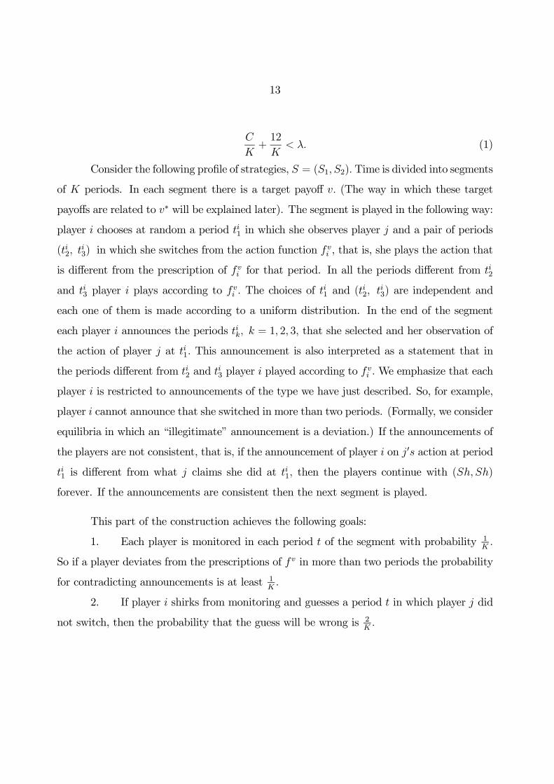
Consider the following profile of strategies, S = (S1, S2). Time is divided into segments

of K periods. In each segment there is a target payoff v. (The way in which these target

payoffs are related to v∗ will be explained later). The segment is played in the following way:

player i chooses at random a period ti1 in which she observes player j and a pair of periods

(ti2, ti3) in which she switches from the action function f

vi , that is, she plays the action that

is different from the prescription of fvi for that period. In all the periods different from ti2

and ti3 player i plays according to fvi . The choices of t

i1 and (t

i2, t

i3) are independent and

each one of them is made according to a uniform distribution. In the end of the segment

each player i announces the periods tik, k = 1, 2, 3, that she selected and her observation of

the action of player j at ti1. This announcement is also interpreted as a statement that in

the periods different from ti2 and ti3 player i played according to f

vi .We emphasize that each

player i is restricted to announcements of the type we have just described. So, for example,

player i cannot announce that she switched in more than two periods. (Formally, we consider

equilibria in which an “illegitimate” announcement is a deviation.) If the announcements of

the players are not consistent, that is, if the announcement of player i on j0s action at period

ti1 is different from what j claims she did at ti1, then the players continue with (Sh, Sh)

forever. If the announcements are consistent then the next segment is played.

This part of the construction achieves the following goals:

1. Each player is monitored in each period t of the segment with probability 1K.

So if a player deviates from the prescriptions of f v in more than two periods the probability

for contradicting announcements is at least 1K.

2. If player i shirks from monitoring and guesses a period t in which player j did

not switch, then the probability that the guess will be wrong is 2K.

14

3. When K is large the monitoring and switching are sparse so the average payoff

in a segment is close to the target payoff. In particular, the average cost of monitoring per

period, CK, is small.

It follows from 1 and 2 that if a player deviates the probability of punishment is at

least 1K. As we will see soon, even when K is large, it is not worthwhile to risk a punishment

when δ is high enough.

To complete the construction of the equilibrium S we need to show how to tailor

different segments together so that the given payoff v∗ ∈ V ∗ can be implemented. Second,we have to construct the equilibrium so that each player is indifferent to the periods in which

she monitors and switches, (otherwise she will not pick these periods at random.) This is

done as follows:

The target payoff of the first segment is v∗, the target payoff of the second segment

is v(2) = v∗ + ε(2) where ε(2) depends on the announcements of the players in the first

segment and precisely offsets the net cost12 of monitoring and switching in the first segment.

Specifically, let a(t) denote the profile of actions that was played in period t according to

the announcements of the players at the end of the segment and let a(t) denote the profile

of actions that were prescribed by the action function fv∗in period t. Define:

xi(t) ≡ gi(a(t))− gi(a(t)).

Thus, xi(t) is the cost (which might be negative) of switching at period t for player

i. (Note that in equilibrium xi(t) is zero if t 6= ti2, ti3, i = 1, 2.) It follows that the net costof monitoring and switching for player i is:

δti1C +

K−1Xt=0

δtxi(t).

12This net cost might be negative.

15

We therefore define ε(2) by the following equation:

2K−1Xt=K

δtεi(2) = δti1C +

K−1Xt=0

δtxi(t).

This definition of the term εi(2) makes player i indifferent to the periods in which she

monitors and switches and thus ensures that choosing these periods randomly is consistent

with the equilibrium. Note that inequality (1) and the fact that | xi(t) |= 0 for t 6= ti2, ti3, i =1, 2, and | xi(t) |<− 3 for t = t

i2, t

i3, i = 1, 2, imply that if δ is sufficiently close to 1, then

| ε(2) |< λ so that v(2) = v∗ + ε(2) ∈ V ∗. Thus, v(2) is a feasible payoff.The target payoffs of subsequent segments are defined in a similar way. Thus, the

target payoff in a segment k is v∗+ ε(k) where the ε(k) term depends on the announcements

of the players at the end of the k−1 segment and precisely offsets the net cost of monitoringand switching at that segment. Thus, the term ε(k) makes player i indifferent to the periods

in which she monitors and switches in the segment k − 1. Also, inequality (1) implies thatall the target payoffs are in the set of feasible payoffs.

We now show that the expected payoff in S = (S1, S2) is v∗. To see that note that

the payoff of player i in the `0th segment, seg(`), in units of the first period of the segment

can be written as:

K−1Xt=0

δt · v∗i +K−1Xt=0

δt · εi(`) +Ri(`)

where Ri (`) is the net cost of switching and monitoring in seg(`) and the εi(`) term is the

term that offsets the net cost of monitoring and switching in seg(`− 1). Thus Ri(`) is offsetby the εi(` + 1) term and the εi(`) term is offset by Ri(`− 1). It follows that the expectedpayoff of player i in S is (1− δ)

P∞t=0 δ

tv∗i = v∗i .

We have completed the definition of S = (S1, S2) and have shown that it generates

the payoff vector v∗. We now show that there exists δ = δ(K) such that for every δ ≤ δ < 1

16

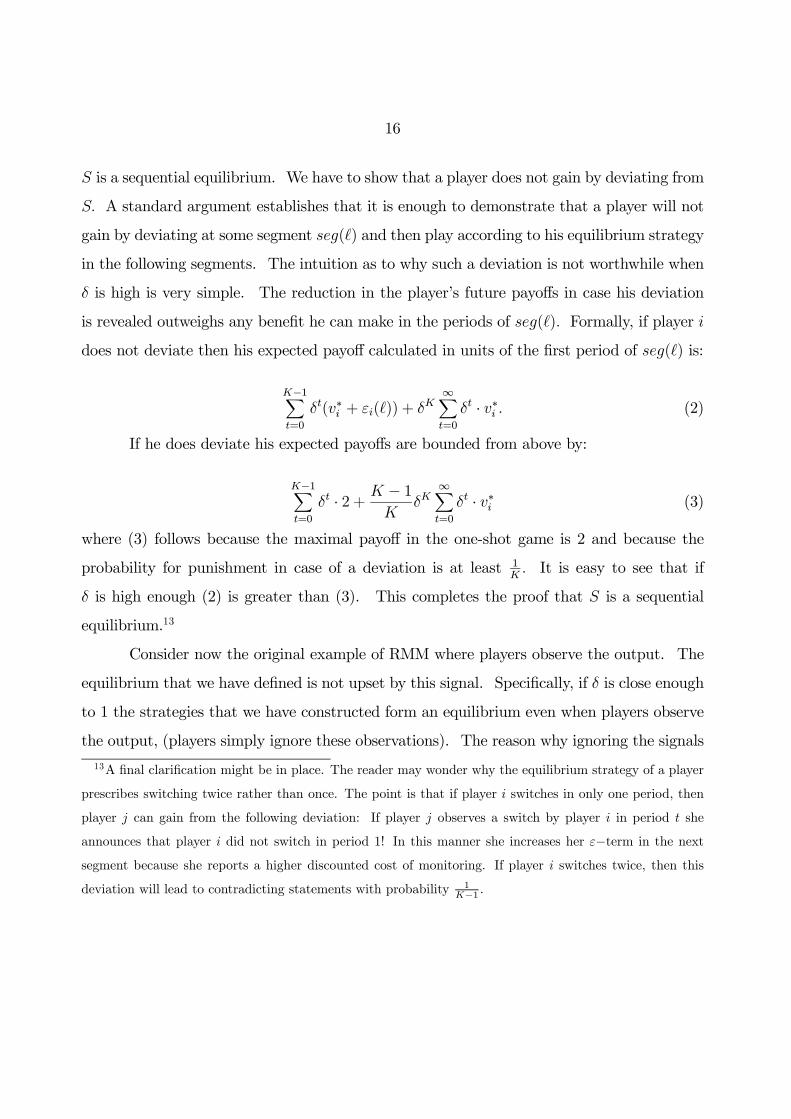
S is a sequential equilibrium. We have to show that a player does not gain by deviating from

S. A standard argument establishes that it is enough to demonstrate that a player will not

gain by deviating at some segment seg(`) and then play according to his equilibrium strategy

in the following segments. The intuition as to why such a deviation is not worthwhile when

δ is high is very simple. The reduction in the player’s future payoffs in case his deviation

is revealed outweighs any benefit he can make in the periods of seg(`). Formally, if player i

does not deviate then his expected payoff calculated in units of the first period of seg(`) is:

K−1Xt=0

δt(v∗i + εi(`)) + δK∞Xt=0

δt · v∗i . (2)

If he does deviate his expected payoffs are bounded from above by:

K−1Xt=0

δt · 2 + K − 1K

δK∞Xt=0

δt · v∗i (3)

where (3) follows because the maximal payoff in the one-shot game is 2 and because the

probability for punishment in case of a deviation is at least 1K. It is easy to see that if

δ is high enough (2) is greater than (3). This completes the proof that S is a sequential

equilibrium.13

Consider now the original example of RMM where players observe the output. The

equilibrium that we have defined is not upset by this signal. Specifically, if δ is close enough

to 1 the strategies that we have constructed form an equilibrium even when players observe

the output, (players simply ignore these observations). The reason why ignoring the signals

13A final clarification might be in place. The reader may wonder why the equilibrium strategy of a player

prescribes switching twice rather than once. The point is that if player i switches in only one period, then

player j can gain from the following deviation: If player j observes a switch by player i in period t she

announces that player i did not switch in period 1! In this manner she increases her ε−term in the next

segment because she reports a higher discounted cost of monitoring. If player i switches twice, then this

deviation will lead to contradicting statements with probability 1K−1 .

17

is consistent with equilibrium behavior is that the signals are imperfect, player i cannot

tell from her observation of the output what player j did and therefore she must monitor j

at some period. Specifically, if player i deviates by shirking from monitoring and guesses the

action of j in some period, relying only on her signals, the probability that player i will be

wrong is bounded from below by some number ρ > 0. When δ is close enough to 1 the loss

that player i will incur in case she is wrong outweighs the cost of monitoring so that even

when ρ is small it is not worthwhile to shirk from monitoring.

The general results that we will obtain in sections 4 and 5 for the case where there

are no signals can be extended to the case of public or private signals in the same manner

provided that the signals have a common support. The significance of this assumption is

that signals are imperfect so that a player cannot determine the action of another player

with certainty. This imperfection ensures that player i has an incentive to monitor. If,

by contrast player i had a perfect signal, sig, on the action of the player j she monitors, so

that when player i observes sig, she knows with certainty the action of player j, then player

i would have had no incentive to monitor j. In such a case player i prefers to wait until she

observes sig and report the action of player j at that period.

4 Three or More Players

In this section theorem 1 is proved for the case of three players or more. So let v∗ ∈ IntV ∗.We will construct a sequential equilibrium with payoff v∗.

To simplify the description of the equilibrium we will assume that the minmax profiles

of actions mi, i ∈ N are pure. The extension to the general case is simple and is provided

in the appendix.

The building blocks of the equilibrium are segments with a finite number of periods.

18

There are K-period and L-period segments. (The L-period segments are used to minmax

one of the players). A segment, seg, is characterized by a target payoff v and a monitoring

assignment q : N → N such that q(i) 6= i. So each player i has another player q(i) whichmonitors him. The segment implements an average payoff that is ‘close’ to v and ensures

that if one of the players deviates from the equilibrium strategies then she is caught with

a probability of at least 1Mwhere M = K,L is the length of the segment. Specifically the

segment is played as follows: player i plays the action function f vi in each period with the

following exception: Player i chooses at random a pair of periods (t1i , t2i ) in which she plays

some action that is different from the action prescribed by f vi . In addition, if player imonitors

another player k, then player i chooses at random a period tk in which she observes player k.

The choices of the tk and (t1i , t2i ) are independent and each one of them is made according to

the uniform distribution. At the end of the segment each player i announces the periods t1i

and t2i in which she switched from playing according to fvi , her pure actions at these periods,

and her observations of the players that she monitored. (So, if she monitors player k she

will announce the period tk and the action of player k at that period.) This announcement

is also interpreted as a statement that, in all periods different from t1i and t2i , player i played

according to fvi .We emphasize that player i is restricted to such announcements. Specifically,

she cannot announce that she switched in more than two periods or that she did not monitor

a player k which was assigned to her. (Formally, an ”illegitimate” message will be considered

a deviation).

Now it is easy to see that if player i deviates from the equilibrium behavior, (either by

lying about her action in a certain period, or by guessing the action of the player she monitors

instead of actually observing him), then with a probability of at least 1Mher announcement

will be inconsistent with the announcement of some other player. (The argument is similar

to the one in the example in section 3). In such a case player i and the player that she

19

contradicted will be punished in the segments that follow the current one.

Next, note that with the exception of at most 3N periods (three periods for each

player), the expected payoff vector in every other period is v. It follows that if K and δ are

large, the expected average payoff on the segment is close to v.

We can now turn to a complete description of a profile of strategies S = (S1, ..., Sn)

which is a sequential equilibrium with an expected payoff v∗. For this purpose it is convenient

to introduce the notion of a ’phase’. A phase is a sequence of segments such that the

announcements in each segment are consistent. A transition from one phase to another

occurs whenever there is a mismatch between the announcements of some player and her

monitor. If there is more than one pair of players that contradict each other then one pair of

the set of contradicting pairs is selected at random. (Each pair with an equal probability).

There are two types of phases. The first type are phases r(v) in which the expected

payoff is v and each phase is composed of a sequence of K− period segments. This set ofphases consists of the initial phase r(v∗), and then, for every pair of players i, j, there is a

phase r(v∗i,j) where v∗i,j is defined as follows: The payoffs of players i and j are v

∗i − η and

v∗j − η respectively and the payoff of a player k 6= i, j is v∗k. Thus, r(v∗i,j) is a phase in whichplayers i and j are punished by reducing their payoffs by η > 0. Note that since v∗ ∈ IntV ∗we can choose η > 0 so that v∗i,j ∈ IntV ∗ for every pair i, j. In fact we want to choose η so

that v∗i − 2η > 0 for every i ∈ N. The second type of phases are phases ri,j in which player iis first minmaxed for L periods and then in the subgame that follows the payoffs of players

i and j are approximately vi − 2η and vj − η respectively. (By approximately we mean that

there is a certain correction term which can be made negligible in comparison to η).

Before providing a detailed description of each phase it is worthwhile to see the general

structure of the equilibrium as it is reflected by the transition rule. The basic idea is simple

if the announcements of two players i and j contradict each other then one of them has

20

deviated and since it is unknown which one of them it was both are punished. Now, since it

is, in general, impossible to punish the same pair of players repeatedly (due to the fact that

it is, in general, impossible to jointly minmax a pair of players), the monitoring assignment

changes from one phase to the other so that in a phase where players i and k are punished

(r(v∗i,k), ri,k.or rk,i) they do not monitor each other and therefore if there will be contradicting

statements in this phase they will involve a pair of players which is different from (i, k).14

The transition rule is defined as follows: If player i and her monitor j make contradicting

statements, (which implies that one of them has deviated), then the next phase is r(v∗i,j)

unless one of them, say, i, is already punished in the current phase (i.e., the current phase

is r(v∗i,k), r(i,k) or r(k,i) for some k 6= i, j) in this case the next phase is r(i,j).(So player i is,first, minmaxed and after that the payoffs of i and j are reduced by η).

We now turn to a full definition of the different phases. Consider first a phase r(v)

(v ∈ Int V ∗). This phase is defined by a sequence of K−period segments (seg(`)∞`=1. Thetarget payoff of seg(1), v(1), is v and the target payoff of seg(`),v(`), is v + ε(`) where the

term ε(`) offsets the net costs of monitoring and switching in the previous segment, seg(`−1).Specifically let t denote the period t in the segment seg(` − 1). Let Ci(t) denote the costincurred by player i for monitoring in period t according to the announcement of player i.

(Ci(t) is zero unless player i says that she monitored in t). Let a(t) denote the profile of

actions that were played in period t according to the announcements of the players, and let

a(t) denote the profile of actions that were prescribed by fv(`−1) in t. Define:

xi(t) = gi(a(t))− gi(a(t))

The term xi(t) is the cost (which might be negative) of the switching at period t

for player i, (when no player switches xi(t) = 0). The term ε(`) is defined by the following

14So if (`,m) are a pair of players that contradict each other in a phase where i and k are punished, then

either ` 6= i, k or m 6= i, k.

21

equation:

2K−1Xt=K

δtεi(`) =K−1Xt=0

δt (Ci(t) + xi(t)))

This definition of the term ε(`) achieves two goals. First, it makes player i indifferent

to the periods in which she monitors and switches and in this way ensures that choosing

randomly the periods of monitoring and switching is consistent with equilibrium. Second,

the expected discounted payoff in the phase is v. (To see that recall the example).

Finally, note that since each player monitors in one period and switches only twice

Ci(t) + xi(t) equals zero except for at most 3N periods. It follows that εi(`) can be made

as small as we wish by taking K and δ to be large enough and therefore v + ε(`) can be

assumed to be a member of the set of feasible and individually rational payoffs, V ∗.15

Consider, now, the phase r(i,j). The phase is a sequence of segments (seg(`))∞`=1. The

segment seg(1) is an L−period segment in which player i is minmaxed. The target payoffin seg(1) is g(mi), (recall that mi is the profile of action that minmaxes player i) and player

i does not monitor and is not monitored. Thus the monitoring assignment is restricted to

the set of players different from i. (Note that there is no need to monitor player i because

his action in the profile mi is a best response). The segments that follow are K−periodsegments in which the monitoring assignment has the property that i and j do not monitor

each other. Let v(i,j) denote the payoff vector where the payoff of player i is v∗i − 2η, thepayoff of player j is v∗j − η, and the payoff of a player k, k 6= i, j is v∗k. The target payoff ofseg(`), ` ≥ 2, is v(i,j) + ε(`) where ε(`) offsets the costs of monitoring and switching in the

previous segment, seg(`− 1).We have completed the definition of the profile S = (S1, ..., Sn). We now show that

we can choose the parameters K,L, and η so that there exists a number δ < 1 such that for15The K and δ which ensure that the ε− terms are below a given term ε are an increasing function of the

cost C and the number of players, N.

22

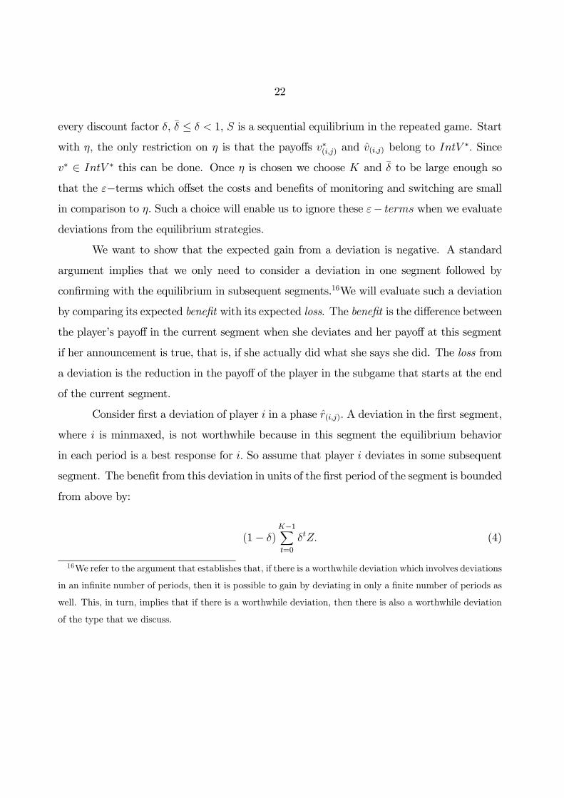
every discount factor δ, δ ≤ δ < 1, S is a sequential equilibrium in the repeated game. Start

with η, the only restriction on η is that the payoffs v∗(i,j) and v(i,j) belong to IntV∗. Since

v∗ ∈ IntV ∗ this can be done. Once η is chosen we choose K and δ to be large enough so

that the ε−terms which offset the costs and benefits of monitoring and switching are smallin comparison to η. Such a choice will enable us to ignore these ε− terms when we evaluatedeviations from the equilibrium strategies.

We want to show that the expected gain from a deviation is negative. A standard

argument implies that we only need to consider a deviation in one segment followed by

confirming with the equilibrium in subsequent segments.16We will evaluate such a deviation

by comparing its expected benefit with its expected loss. The benefit is the difference between

the player’s payoff in the current segment when she deviates and her payoff at this segment

if her announcement is true, that is, if she actually did what she says she did. The loss from

a deviation is the reduction in the payoff of the player in the subgame that starts at the end

of the current segment.

Consider first a deviation of player i in a phase r(i,j). A deviation in the first segment,

where i is minmaxed, is not worthwhile because in this segment the equilibrium behavior

in each period is a best response for i. So assume that player i deviates in some subsequent

segment. The benefit from this deviation in units of the first period of the segment is bounded

from above by:

(1− δ)K−1Xt=0

δtZ. (4)

16We refer to the argument that establishes that, if there is a worthwhile deviation which involves deviations

in an infinite number of periods, then it is possible to gain by deviating in only a finite number of periods as

well. This, in turn, implies that if there is a worthwhile deviation, then there is also a worthwhile deviation

of the type that we discuss.

23

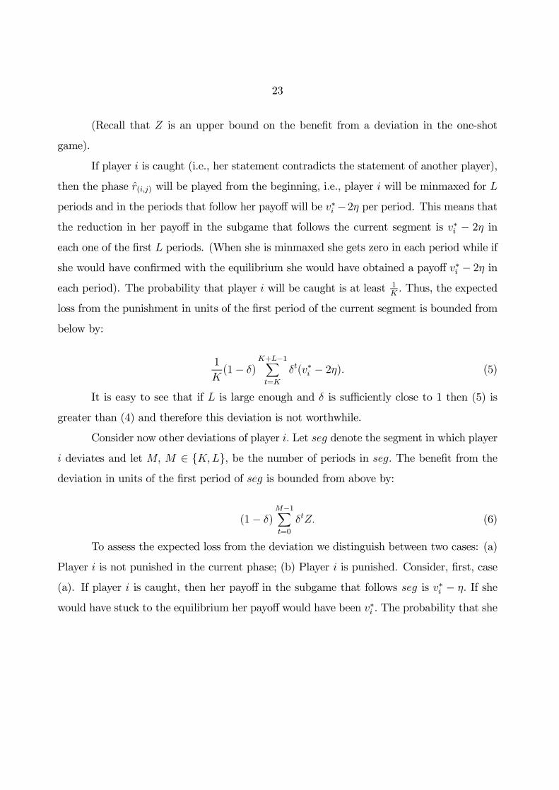
(Recall that Z is an upper bound on the benefit from a deviation in the one-shot

game).

If player i is caught (i.e., her statement contradicts the statement of another player),

then the phase r(i,j) will be played from the beginning, i.e., player i will be minmaxed for L

periods and in the periods that follow her payoff will be v∗i −2η per period. This means thatthe reduction in her payoff in the subgame that follows the current segment is v∗i − 2η ineach one of the first L periods. (When she is minmaxed she gets zero in each period while if

she would have confirmed with the equilibrium she would have obtained a payoff v∗i − 2η ineach period). The probability that player i will be caught is at least 1

K. Thus, the expected

loss from the punishment in units of the first period of the current segment is bounded from

below by:

1

K(1− δ)

K+L−1Xt=K

δt(v∗i − 2η). (5)

It is easy to see that if L is large enough and δ is sufficiently close to 1 then (5) is

greater than (4) and therefore this deviation is not worthwhile.

Consider now other deviations of player i. Let seg denote the segment in which player

i deviates and let M, M ∈ K,L, be the number of periods in seg. The benefit from the

deviation in units of the first period of seg is bounded from above by:

(1− δ)M−1Xt=0

δtZ. (6)

To assess the expected loss from the deviation we distinguish between two cases: (a)

Player i is not punished in the current phase; (b) Player i is punished. Consider, first, case

(a). If player i is caught, then her payoff in the subgame that follows seg is v∗i − η. If she

would have stuck to the equilibrium her payoff would have been v∗i . The probability that she

24

is caught is at least 1M. It follows that the expected loss from the deviation in units of the

first period of seg is bounded from below by:

1

M(1− δ)

∞Xt=M

δtη. (7)

It is easy to see that if δ is close enough to 1 (7) is greater than (6) and therefore the

deviation is not worthwhile.

Consider now Case (b). If the deviation of player i is revealed, then player i is

punished by being minmaxed for L periods and then getting an expected payoff v∗i − 2ηin each period. If player i would have confirmed with the equilibrium her expected payoff

would have been v∗i − η in each period that follows seg. It follows that in the first L periods

the loss is v∗i − η per period and after that it is η per period. Since v∗i − η > η we get that

the expected loss in this case is bounded from below by (7) as well. Therefore we obtain

again that if δ is close to 1 the deviation is not worthwhile.

We have shown that S is a sequential equilibrium17 and have thus proved that every

payoff vector v∗ in which the payoff of each player is above her minmax payoff in pure

actions can be implemented in a sequential equilibrium. In the appendix we show how the

proof can be easily extended for payoff vectors in which the payoff of each player is above

her minmax payoff in mixed actions.

17There is still room for some clarifying comments regarding: 1) Deviations where a player observes other

players more than once. 2. The beliefs of players outside the equilibrium path. These comments are

marginal to the main ideas in the construction and therefore they are delegated to the appendix.

25

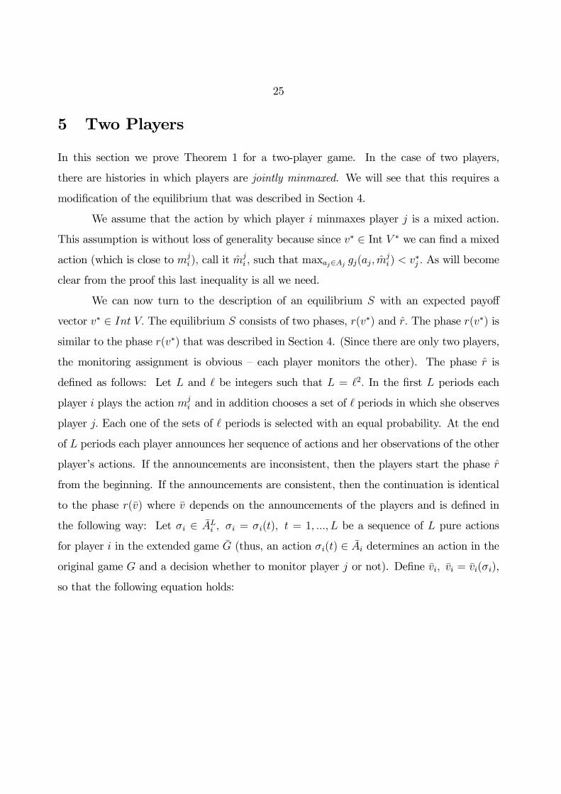
5 Two Players

In this section we prove Theorem 1 for a two-player game. In the case of two players,

there are histories in which players are jointly minmaxed. We will see that this requires a

modification of the equilibrium that was described in Section 4.

We assume that the action by which player i minmaxes player j is a mixed action.

This assumption is without loss of generality because since v∗ ∈ Int V ∗ we can find a mixedaction (which is close to mj

i ), call it mji , such that maxaj∈Aj gj(aj, m

ji ) < v

∗j . As will become

clear from the proof this last inequality is all we need.

We can now turn to the description of an equilibrium S with an expected payoff

vector v∗ ∈ Int V. The equilibrium S consists of two phases, r(v∗) and r. The phase r(v∗) issimilar to the phase r(v∗) that was described in Section 4. (Since there are only two players,

the monitoring assignment is obvious — each player monitors the other). The phase r is

defined as follows: Let L and ` be integers such that L = `2. In the first L periods each

player i plays the action mji and in addition chooses a set of ` periods in which she observes

player j. Each one of the sets of ` periods is selected with an equal probability. At the end

of L periods each player announces her sequence of actions and her observations of the other

player’s actions. If the announcements are inconsistent, then the players start the phase r

from the beginning. If the announcements are consistent, then the continuation is identical

to the phase r(v) where v depends on the announcements of the players and is defined in

the following way: Let σi ∈ ALi , σi = σi(t), t = 1, ..., L be a sequence of L pure actions

for player i in the extended game G (thus, an action σi(t) ∈ Ai determines an action in theoriginal game G and a decision whether to monitor player j or not). Define vi, vi = vi(σi),

so that the following equation holds:

26

(1− δ)

"L−1Xt=0

δtgi(σi(t),mij) +

∞Xt=L

δtvi

#

= (1− δ)

"L−1Xt=0

δt · 0 +∞Xt=L

δtv∗i

#= δLv∗i.

Thus, for every sequence of pure actions in the extended game, σi, player i is indiffer-

ent between playing σi in the minmax segment and receiving afterwards a payoff vi in each

period, and the path of one-shot payoffs P in which she receives 0 in the first L periods and

v∗i in every subsequent period. In particular, player i is indifferent among her pure actions in

the original game G and indifferent to the set of periods in which she observes player j. Note

that: (i) since gi(ai,mij) <− 0 for every ai ∈ Ai, di(σi) = vi(σi) − v

∗i >− 0 for every σi; (ii)

di(σi) can be as small as we wish for every σi if δ is sufficiently close to 1. So if v∗ ∈ Int Vwe can assume that v ∈ V and therefore v is a feasible payoff.

We now show that there is an L such that there exists a δ so that, for every δ > δ, S

is a sequential equilibrium. We need to consider two types of deviations:

(i) a deviation of a player in the minmax segment of the phase r

followed by confirming with the equilibrium after the end of the segment;

(ii) a deviation at any other segment followed, again, by confirming with

the equilibrium

It will become apparent that in evaluating these deviations we need to consider only

a finite horizon which consists of the segment in which the deviation occurs and the L periods

which follow it. Since δ is as close to 1 as we wish the effect of the discounting in this finite

horizon is negligible and can be ignored. Thus, we can evaluate a deviation in terms of

one-shot payoffs. So, for example, we will evaluate a payoff x in each of h periods by h · x.Also, in evaluating a deviation we will ignore, (as we did in section 4), the ε−terms

that offset the costs of monitoring and switching in K−period segments. These terms can

27

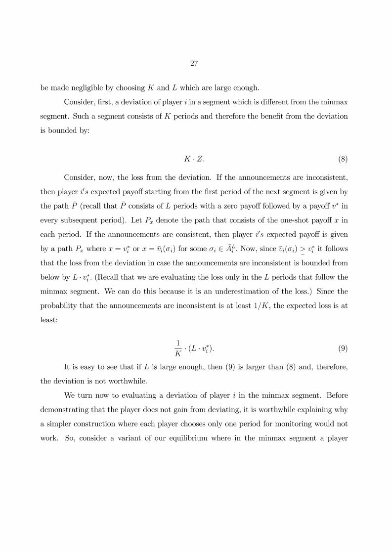
be made negligible by choosing K and L which are large enough.

Consider, first, a deviation of player i in a segment which is different from the minmax

segment. Such a segment consists of K periods and therefore the benefit from the deviation

is bounded by:

K · Z. (8)

Consider, now, the loss from the deviation. If the announcements are inconsistent,

then player i0s expected payoff starting from the first period of the next segment is given by

the path P (recall that P consists of L periods with a zero payoff followed by a payoff v∗ in

every subsequent period). Let Px denote the path that consists of the one-shot payoff x in

each period. If the announcements are consistent, then player i0s expected payoff is given

by a path Px where x = v∗i or x = vi(σi) for some σi ∈ ALi . Now, since vi(σi) >− v∗i it follows

that the loss from the deviation in case the announcements are inconsistent is bounded from

below by L · v∗i . (Recall that we are evaluating the loss only in the L periods that follow theminmax segment. We can do this because it is an underestimation of the loss.) Since the

probability that the announcements are inconsistent is at least 1/K, the expected loss is at

least:

1

K· (L · v∗i ). (9)

It is easy to see that if L is large enough, then (9) is larger than (8) and, therefore,

the deviation is not worthwhile.

We turn now to evaluating a deviation of player i in the minmax segment. Before

demonstrating that the player does not gain from deviating, it is worthwhile explaining why

a simpler construction where each player chooses only one period for monitoring would not

work. So, consider a variant of our equilibrium where in the minmax segment a player

28

chooses only one period in which she monitors the other player. Let ai and a0i be two pure

actions for player i in G such that:

yi ≡ gi(ai,mij)− gi(a0i,mi

j) > v∗i .

Consider a deviation where player i lies and announces that at some period t she

played a0i while in fact she played the action ai. Assume that this is the only deviation of

player i. The gain from the deviation if player i is not caught, that is, if the announcements

at the end of the segment are consistent, is yi. To evaluate the loss, note that the expected

payoff of player i starting with the first period of the next segment is v∗i . If player i is caught,

then she will be minmaxed for L periods and therefore her loss in this case is L · v∗i . Theprobability that player i will be caught is 1/L. It follows that expected loss is v∗i while the

expected gain is ((L− 1)/L) · yi. Thus, if L is large the deviation is worthwhile.We now show that a choice of ` =

√L periods of monitoring works and that S is

an equilibrium. We will evaluate a deviation of player i by comparing her gain from the

deviation in case she is not caught (that is, the case where the announcements at the end of

the segment are consistent), with her loss in case she is caught.

Let−ai,

−a0i∈−Aibe pure actions of player i in the extended game. Let yi = gi(ai,mi

j)−gi(a

0i,m

ij). Player i gains yi at period t if she announces that she played a

0i at t while in fact

she played ai at that period, and if she is not caught. Thus, the gain in a single period is

bounded from above by Z and therefore the gain from a deviation in k periods is bounded by

k ·Z. Consider now the loss of player i in case she is caught. If player i would have confirmedwith the equilibrium, then her expected payoff would have been given by the path P in

which she gets 0 for L periods and v∗i in every subsequent period. If player i deviates and is

caught, then her payoff is bounded from above by the payoff that corresponds to the path Pc

in which player i gets 0 for 2L periods and then v∗i in every subsequent period. This follows

because the maximal one-shot payoff of player i in each period in the minmax segment is

29

0 and if she is caught, then the game continues by playing the phase r from the beginning.

It follows that the loss from being caught is bounded from below by L · v∗i . Let p(k) denotethe probability that player i will be caught if she deviates in k periods. It follows that the

deviation is not worthwhile if the following inequality holds:

[1− p(k)]kZ < p(k)Lv∗i . (10)

Claim: There exists L such that (10) holds for every L >− L.

Lemma 2 There exists L such that if L >− L then:

p(k) >− 1−"µ1− 1

`

¶k#. (11)

Proof. It will be shown that:

1− p(k) <−µ1− 1

`

¶k. (12)

There are two types of deviations: (i) shirking from monitoring and (ii) giving a false

announcement regarding the pure action in the original game G, ai(t) ∈ Ai, that was playedin some period t.

Let aj and a0j, aj, a0j ∈ Aj, denote respectively two pure actions in the support of mi

j

which are assigned the highest and lowest probabilities, respectively. Let pj and p0j denote

these probabilities, respectively. Now, assume that player i monitors player j in only `− 1periods. Since player i must report on the actions of player j in ` periods her optimal

continuation is to select some additional period t and announce that she observed player j in

period t and that player j played the action aj. The probability that player i will be wrong

is at least p0j. If L is large enough, p0j >− 1/` and our claim follows for k = 1, (the case where

player i shirks in only one period). Suppose, now, that player i shirks in k periods where

30

k > 1. If player i is not caught at the end of the segment, then player i guessed correctly the

actions of player j in k periods. The probability of that is at most³1− p0j

´ksince p0j >− 1/`,

(12) follows.

Now suppose that player i deviates by lying about his pure action ai(t) ∈ Ai in someperiod t. Player i is caught if player j monitors player i at t. The probability of that is

`/L = 1/`. So our claim follows for k = 1. If player i lies about her actions in k periods then

the probability that she will not be caught is:

k−1Yh=0

Ã1− `

L− h!. (13)

Since (13) is lower than the r.h.s. of (12) the lemma follows.

We can now turn to the proof of the claim.

Let

λ ≡ v∗i

Z

and let θ be the smallest number such that θ ≥ λ

and

2e−θ

1− e−θ <v∗iZ

(14)

where e is the basis of the natural logarithm. Consider the following three cases:

1. 1 <− k <− λ`.

2. λ` <− k <− θ`.

3. θ` < k.

We have p(k) >− p(1) >− 1/` for every k >− 1. Thus, for 1 <− k <− λ` we have:

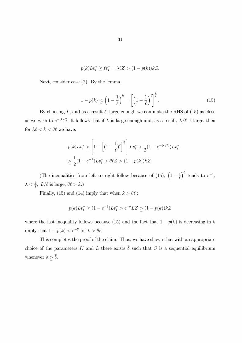
31

p(k)Lv∗i ≥ `v∗i = λ`Z > (1− p(k))kZ.

Next, consider case (2). By the lemma,

1− p(k) <−µ1− 1

`

¶k=

"µ1− 1

`

¶`#k`. (15)

By choosing L, and as a result `, large enough we can make the RHS of (15) as close

as we wish to e−(k/`). It follows that if L is large enough and, as a result, L/` is large, then

for λ` <− k <− θ` we have:

p(k)Lv∗i >−

1− ·(1− 1`)`¸k`

Lv∗i >− 12(1− e−(k/`))Lv∗i .>−1

2(1− e−λ)Lv∗i > θ`Z > (1− p(k))kZ

(The inequalities from left to right follow because of (15),³1− 1

`

´`tends to e−1,

λ < k`, L/` is large, θ` > k.)

Finally, (15) and (14) imply that when k > θ` :

p(k)Lv∗i ≥ (1− e−θ)Lv∗i > e−θLZ >− (1− p(k))kZ

where the last inequality follows because (15) and the fact that 1− p(k) is decreasing in kimply that 1− p(k) <− e

−θ for k > θ`.

This completes the proof of the claim. Thus, we have shown that with an appropriate

choice of the parameters K and L there exists δ such that S is a sequential equilibrium

whenever δ >− δ.

32

6 Conclusion

We have shown that V (G) contains the interior of V ∗. A complete characterization of V (G)

seems to be difficult to obtain and is beyond the scope of this paper. However, in this section

we make a few observations that are related to this problem.

Let bvi denote the minmax payoff for player i in G when the players different from i

can correlate their actions against i. That is,

bvi = minβ−i∈∆(A−i)

maxai∈Ai

gi(ai,β−i)

Let β−i ∈ ∆(A−i) be a probability distribution such that maxai gi(ai, β−i) = bvi.Define:

W = w ∈ Rn | ∃v ∈ V, bvi ≤ wi ≤ vi, i = 1, .., nWe claim that V (G) ⊆W.To see that we, first, observe that given a profile of strategies in the repeated game,

S−i, player i can guarantee a payoff of at least bvi as follows: Player i never spends moneyon observing the actions of the other players. Let β1−i ∈ ∆ (A−i) denote the probability

distribution on the profiles of actions of the players different from i in the original game G

in the first period. The action of player 1 in the first period is a1i where

a1i = arg maxai∈Ai

gi(ai,β1−i)

Assume that a1i , ...., at−1i have been defined. Let βt−i denote the probability distribu-

tion on the profile of the actions of the players different from i in period t given that player

i played a1i , ...., at−1i in the first t− 1 periods. Define:

ati = arg maxai∈Ai

gi(ai, βt−i)

33

It is easy to see that in each period t player i gets an expected payoff of at least bviand therefore he gets at least bvi in the repeated game.

Next, we observe that a payoff, w, in the repeated game G(δ) can be represented as

w = v − c where v ∈ V is the corresponding payoff in the repeated game G(δ) and c is thediscounted sum of the costs of monitoring in the different periods.

These two observations establish the claim.

We note that the set W is different from the set of individual rational payoffs, V ∗, in

two ways. Let w ∈W then,

1. wi may be smaller than vi, the individual rational payoff for player i.

2. The vector w may not belong to V, the convex hull of the set of payoff vectors in

G.

We now show that V (G) may indeed differ from V ∗ in these two ways. To see 1.

consider a 4-person game in which player 1 does not observe anything for free, not even his

payoff, while each one of the other players observes the actions of all the players for free.

We will show that if the cost for player 1 of observing the actions of any other player is

sufficiently high then it is possible to implement in equilibrium a payoff vector w such that

wi is ”close” to bvi .The idea is simple; If player 1 deviates in some period bt then the otherplayers correlate their actions against him for some number of periods, L, that is large enough

to offset the gain of player 1 in period bt. This is done in the following way: Assume w.l.o.g.that |A2| ≥ |Aj| for j = 3, 4. Player 2 conducts a private lottery according to the probabilitydistribution β−1 on A−1. (Recall that β−1 is a probability distribution such that maxa1g1(a1,

β−1) = bvi. ) Let (a2, a3, a4) be the outcome of the lottery. Since |A2| ≥ |Aj| for j = 3, 4

player 2 can communicate aj to player j in one period. Specifically, let fj,fj : Aj → A2,

be some bijection of Aj into A2. Player 2 communicates aj to player j by playing fj(aj) in

period bt + (j − 2). So after two periods players 3 and 4 know a3 and a4 and starting with

34

period bt+3 players 2,3 and 4 play (a2, a3, a4) for L periods where L is large enough to offsetthe gain of player 1 from the deviation in period bt. Now the point is this, if the cost forplayer 1 of observing any action of any other player is high enough then it is not worthwhile

for him to make any observation in any period t, bt + 1 ≤ t ≤ bt + L + 2. If player 1 doesn’tobserve any action he has no information on the actions of the other players and therefore

his maximal expected payoff in each period t in the punishment segment is cv1. Since alongthe equilibrium path player 1 gets an expected payoff w1 in each period, where w1 Â cv1, thenif L is large enough the deviation is not worthwhile.

We have shown that V (G) may contain points in which the payoffs of some of the

players are below their individual rational payoffs. The set V (G) may also contain points

which do not belong to V. To see that we note, without proof, that there are equilibria, which

are similar to the equilibria that were defined in section 4, in which some (or all) players

observe other players many times in each segment so that the average cost of monitoring

per period is not negligible. Thus, it is possible to diminish the payoff of players by forcing

them to spend money on monitoring. In particular, given a n-person game G a vector v ∈V ∗ and a vector α = (α1, .....,αn) such that 0≺ αi ≤ 1, i = 1, .., n, there exist cost functionsCi, i = 1, .., n, such that the payoff vector α · v belongs to V (G).

35

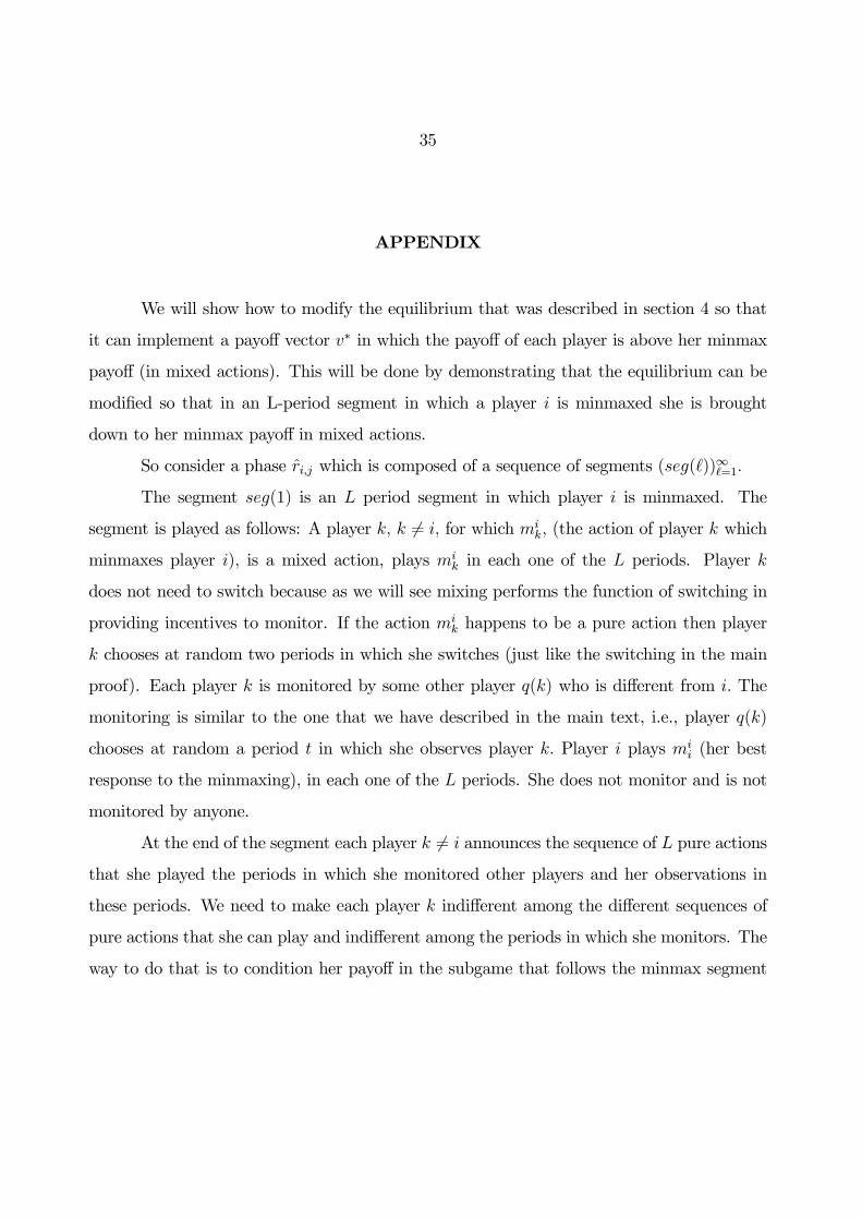
APPENDIX

We will show how to modify the equilibrium that was described in section 4 so that

it can implement a payoff vector v∗ in which the payoff of each player is above her minmax

payoff (in mixed actions). This will be done by demonstrating that the equilibrium can be

modified so that in an L-period segment in which a player i is minmaxed she is brought

down to her minmax payoff in mixed actions.

So consider a phase ri,j which is composed of a sequence of segments (seg(`))∞`=1.

The segment seg(1) is an L period segment in which player i is minmaxed. The

segment is played as follows: A player k, k 6= i, for which mik, (the action of player k which

minmaxes player i), is a mixed action, plays mik in each one of the L periods. Player k

does not need to switch because as we will see mixing performs the function of switching in

providing incentives to monitor. If the action mik happens to be a pure action then player

k chooses at random two periods in which she switches (just like the switching in the main

proof). Each player k is monitored by some other player q(k) who is different from i. The

monitoring is similar to the one that we have described in the main text, i.e., player q(k)

chooses at random a period t in which she observes player k. Player i plays mii (her best

response to the minmaxing), in each one of the L periods. She does not monitor and is not

monitored by anyone.

At the end of the segment each player k 6= i announces the sequence of L pure actionsthat she played the periods in which she monitored other players and her observations in

these periods. We need to make each player k indifferent among the different sequences of

pure actions that she can play and indifferent among the periods in which she monitors. The

way to do that is to condition her payoff in the subgame that follows the minmax segment

36

on her announcements at the end of the segment so that her total discounted payoff is fixed.

The precise way in which this is done is as follows. Let (A−i)L denote the sequence of profiles

of pure actions of the players different from i in the minmax segment. Let d(A−i)L → RN−1+

be a function such that for any two elements of (A−i)L,σ−i(t) and τ−i(t), t = 1, ..., L, and

every k ∈ N − i, k is indifferent between the path of payoffs that start with the sequencegk(σ−i(t),mi

i), t = 1, ..., L, and continues with a constant payoff d(σ−i(t))k, and the path

of payoffs that starts with the sequence gk(τ−i(t),mii) and continues with constant payoff

d(τ−i(t))k. Now it is easy to see that for any given L and ² > 0, if δ is close enough to

1, we can define d so that for every σ−i(t) ∈ (A−i)L, d(σ−i(t))k is a nonnegative numberwhich is smaller than ². Let Ct be the monitoring cost incurred by player k, according to her

announcement, at period t, 1 <− t <− L, in the minmax segment. Define ²0k by the equation:

∞Xt=L

δt²0k =L−1Xt=0

δt · Ct.

Thus, ²0k is the increase per period in the payoff of k which would precisely compensate

k for her cost of monitoring. Again, it is easy to see that for any L and ² > 0 if δ is close

enough to 1 then ²0k < ².

Define the vector payoff v as follows:

vk = v∗k + d(σ−i(t))k + ²0k, k 6= i, j

vj = v∗j − η + d(σ−i(t))j + ²0j

vi = v∗i − 2η.

If, at the end of the minmax segment, the announcements of the players are consistent, then

the continuation of the phase is identical to the phase r(v) and the monitoring assignment

has the property that players i and j do not monitor each other.

37

If the announcements are inconsistent then the next phase is determined by the

transition rule that was defined in the main proof (that is, the pair of players that contradict

each other are punished).

Some additional clarifying comments to the proof in Section 4 regarding:

1) Deviations where a player observes other players more than once.

2) The beliefs of players outside the equilibrium path.

1. Suppose that player 1 deviates by observing the actions of other players in several,

(or all), periods in a given segment. It is easy to see that player i cannot gain from such a

deviation because player i remains uncertain about the period in which his action is moni-

tored so he has no incentive to deviate by switching more than twice from the prescriptions

of the action function f v.

However, there is an additional potential difficulty in the construction of our equilib-

rium. Consider an out of equilibrium history, h, in which player i has deviated by observing

the actions of all, or some, of the other players in, say, all the periods except the last one

in the current segment, seg. (That is, the period that follows h is the last period in seg).

Assume furthermore that some players different from i have deviated by switching from the

action function more than twice so that player i knows that there is a positive probability

that players different from himself will make contradicting statements at the end of the seg-

ment. (This probability might in fact be close to 1 if, for example, player i observes that

some player j has deviated in all the M − 1 periods, M = K,L, that have been observed.)

Now this might make it worthwhile for player i to deviate from fv in the last period because

the probability that he will be punished is smaller than 1M. Specifically, suppose that player i

has switched twice in the firstM periods of, seg, and now upon observing that other players

have deviated decides to switch for the third time in the last period of seg. To see that

this deviation is in fact not worthwhile recall that in the case where there are several pairs

38

of players that contradict each other the transition function selects at random (from the set

of contradicting pairs), a pair of players to be punished. Now this means that even in the

case where player i observed deviations by other players his decision to deviate at the last

period of seg, (or at any other period), increases the probability that he will be selected for

punishment by at least 1M· 1N. This follows because the probability that the monitor of i,

q(i), will choose to observe i in the last period of seg is 1Mand because there are at most N

pairs of players which can contradict each other (a pair (j, q(j)) for every player j.)

Going back to the proof, we easily observe that for any positive probability p, (in

particular for p = 1M· 1N), there exists L(p) and δ(p) such that if L > L(p) and δ > δ(p)

then it is not worthwhile to deviate when the probability of punishment is greater than

p. Specifically, the arguments on pages 22, 23 and 24 carry through if we substitute 1Kin

expression (5) and 1Min expression (7) by any positive number p.

2. We have not been explicit about the definition of the beliefs outside the equilibrium

path. This deserves a comment. The point is that the beliefs of the players are not really

important, or more precisely, the condition of sequential rationality is satisfied for a general

class of beliefs including all the beliefs which satisfy the condition of consistency. To see

this note that since the game is a repeated game with complete information, that is, there is

no uncertainty about the payoffs in the one-shot game, the only significance of the imperfect

monitoring to the satisfaction of the condition of sequential rationality is the uncertainty that

it generates about the behavior of the players in the continuation of the game. In other words

the beliefs of a player about what happened in the past do not change her optimal behavior

in the continuation of the game as long as her beliefs about the behavior of the players in

the continuation of the game remain the same. Now, the announcements of the players at

the end of each segment18 determine the strategies of the players in the continuation of the

18Plus the outcome of a lottery if several pairs of players contradicted each other.

39

game. So in a period t,1 ≤ t ≤,M in a segment, seg, of length M, M = K,L, the beliefs of

a player i about what happened in the periods that preceded seg are completely irrelevant,

any belief, and in particular beliefs that satisfy consistency, would work. What matters

are the beliefs of player i about the play in seg. The discussion in the previous paragraph

highlights the fact that the only property of the beliefs of player i which is required to make

her strategy an optimal response is that for each period t, t ≥ t, player i assigns a positiveprobability which is bounded from below to being monitored at t. Call this property P.

It is easy to see that each system of beliefs which satisfies consistency satisfies P. Along

the equilibrium path P follows from Bayesian updating and outside the equilibrium path

P follows from belief revision which assumes a minimal number of deviations, (a condition

which is implied by consistency).

40

References

[1] D.Abreu, D.Pearce and E.Stachetti, “Optimal Cartel Equilibria with Imperfect Moni-

toring,” Journal of Economic Theory, 39 (1986), 251-269.

[2] D.Abreu, D.Pearce and E.Stachetti, “Toward a Theory of Discounted Repeated Games

with Imperfect Monitoring,” Econometrica, 58 (1990), 1041-1064.

[3] R.J.Aumann and L.Shapley, “Long-term Competition: A Game Theoretic Analysis,”

mimeo, 1976.

[4] E.Ben-Porath and M.Kahneman, “Communication in Repeated Games with Private

Monitoring,” Journal of Economic Theory, 76 (1996), 281-297.

[5] O. Compte, “Communication in Repeated Games with Imperfect Private Monitoring,”

Econometrica, 66 (1998), 597-626.

[6] E. Green and R. Porter, “Non-Cooperative Collusion under Imperfect Price Informa-

tion,” Econometrica, 52 (1984), 87-100.

[7] D.Fudenberg and D.Levine, “An Approximate Folk Theorem with Imperfect Private

Information,” Journal of Economic Theory, 54 (1991), 26-47.

[8] D.Fudenberg, D.Levine and E.Maskin, “The Folk Theorem with Imperfect Public In-

formation,” Econometrica, 62 (1994), 997-1040.

[9] D.Fudenberg and E.Maskin, “Folk Theorems for Repeated Games with Discounting and

Incomplete Information,” Econometrica, 54 (1986), 533-554.

[10] M.Kandori and H.Matsushima, “Private Observation, Communication and Collusion,”

Econometrica, 66 (1998), 627-652.

41

[11] D.Kreps and R.Wilson, “Sequential Equilibrium,” Econometrica, 50 (1982), 863-894.

[12] E.Lehrer, “Nash Equilibria of n-player Repeated Games with Semi-standard Informa-

tion,” International Journal of Game Theory, 19 (1990).

[13] ___________ “Correlated Equilibria in Two-Player Repeated Games with Nonob-

servable Actions,”Mathematics of Operations Research, 17 (1992), 175-199.

[14] ___________ “Two-Player Repeated Games with Nonobservable Actions and Ob-

servable Payoffs,”Mathematics of Operation Research, 17 (1992), 200-224.*

[15] R.Radner, “Repeated Partnership Games with Imperfect Monitoring and No Discount-

ing,” Review of Economic Studies, 53 (1986), 43-58.

[16] R.Radner, R.Myerson and E.Maskin, “An Example of a Repeated Partnership Game

with Discounting and with Uniformly Inefficient Equilibria,” Review of Economic

Studies, 53 (1986), 59-70.

[17] A.Rubinstein, “Equilibrium in Supergames with the Overtaking Criterion,” Journal

of Economic Theory, 27 (1979), 1-9.