Communication Cost in Parallel Query Processing Dan Suciu University of Washington Joint work with...
50
Communication Cost in Parallel Query Processing Dan Suciu University of Washington Joint work with Paul Beame, Paris Koutris and the Myria Team 1 Beyond MR - March 2015
-
Upload
janis-barton -
Category
Documents
-
view
219 -
download
3
Transcript of Communication Cost in Parallel Query Processing Dan Suciu University of Washington Joint work with...
Beyond MR - March 2015 1
Communication Cost in Parallel Query Processing
Dan Suciu
University of Washington
Joint work with Paul Beame, Paris Koutrisand the Myria Team

This Talk
• How much communication is needed to compute a query Q on p servers?

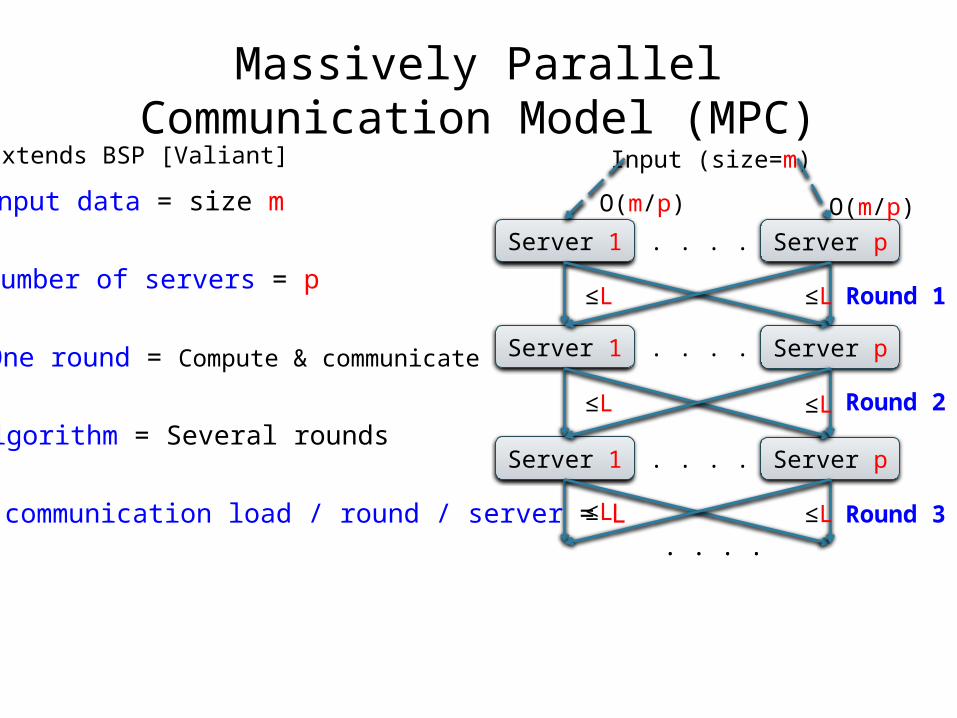
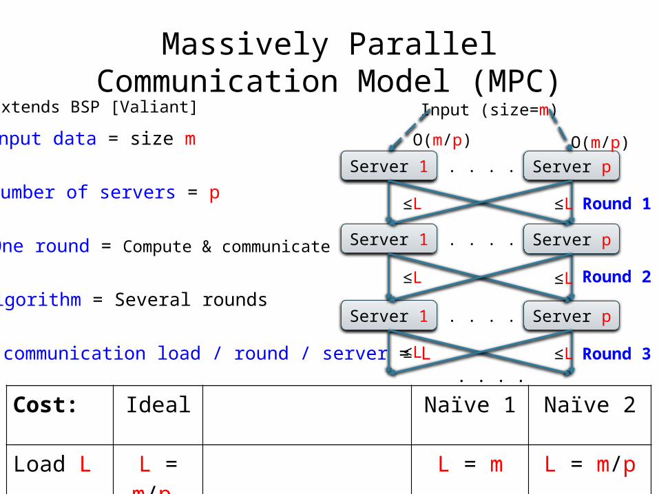
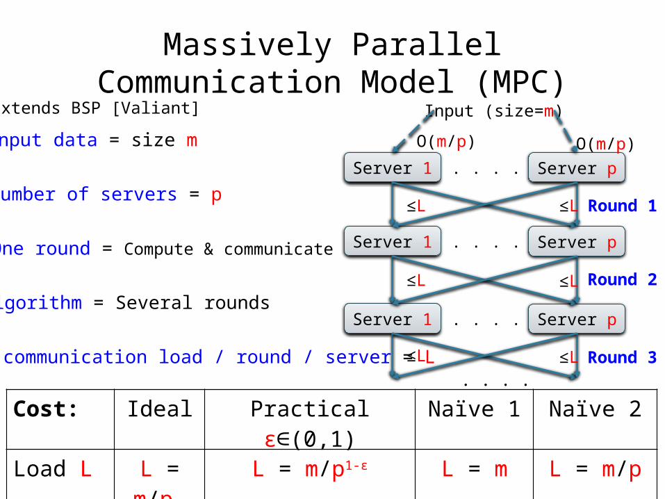
Massively Parallel Communication Model (MPC)
Server 1
Server p
. . . .
Input (size=m)
Input data = size m
Number of servers = p
O(m/p) O(m/p)
Extends BSP [Valiant]

Massively Parallel Communication Model (MPC)
Server 1
Server p
. . . .
Server 1
Server p
. . . .
Input (size=m)
Round 1
Input data = size m
One round = Compute & communicate
Number of servers = p
O(m/p) O(m/p)
Extends BSP [Valiant]
≤L ≤L

Massively Parallel Communication Model (MPC)
Server 1
Server p
. . . .
Server 1
Server p
. . . .
Server 1
Server p
. . . .
Input (size=m)
. . . .
Round 1
Round 2
Round 3. . . .
Input data = size m
Algorithm = Several rounds
One round = Compute & communicate
Number of servers = p
O(m/p) O(m/p)
Extends BSP [Valiant]
≤L
≤L
≤L
≤L
≤L
≤L
Massively Parallel Communication Model (MPC)
Server 1
Server p
. . . .
Server 1
Server p
. . . .
Server 1
Server p
. . . .
Input (size=m)
. . . .
Round 1
Round 2
Round 3. . . .
Input data = size m
Max communication load / round / server = L
Algorithm = Several rounds
One round = Compute & communicate
Number of servers = p≤L
≤L
≤L
≤L
≤L
≤L
O(m/p) O(m/p)
Extends BSP [Valiant]
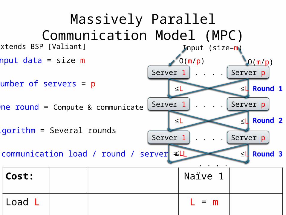
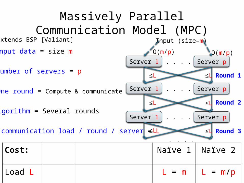
Cost: Ideal Practical ε (0,1)∈ Naïve 1 Naïve 2
Load L L = m/p L = m/p1-ε L = m L = m/p
Rounds r 1 O(1) 1 p
Massively Parallel Communication Model (MPC)
Server 1
Server p
. . . .
Server 1
Server p
. . . .
Server 1
Server p
. . . .
Input (size=m)
. . . .
Round 1
Round 2
Round 3. . . .
Input data = size m
Max communication load / round / server = L
Algorithm = Several rounds
One round = Compute & communicate
Number of servers = p≤L
≤L
≤L
≤L
≤L
≤L
O(m/p) O(m/p)
Extends BSP [Valiant]
Cost: Ideal Practical ε (0,1)∈ Naïve 1 Naïve 2
Load L L = m/p L = m/p1-ε L = m L = m/p
Rounds r 1 O(1) 1 p

12
Example: Join(x,y,z) = R(x,y), S(y,z)
Server 1
Server p
. . . .
R(x,y) ⋈ S(y,z) R(x,y) ⋈ S(y,z)
Output:• Each server computes
the local join R(x,y) ⋈ S(y,z)
Server 1
Server p
. . . .
Round 1
Round 1: each server• Sends record R(x,y) to server h(y) mod p• Sends record S(y,z) to server h(y) mod p
Input: R, S • Uniformly partitioned on p servers
|R|=|S|=m
Load L = O(m/p) w.h.p.Rounds r = 1
Assuming no skew
x y
a b
a c
b c
y z
b d
b e
c e⋈
R S
O(m/p) O(m/p)

13
Speedup
# processors (=p)
SpeedA load of L = m/p corresponds to linear speedup
A load of L = m/p1-ε corresponds to sub-linear speedup

14
Outline
• The MPC Model
• The Algorithm
• Skew matters
• Statistics matter
• Extensions and Open Problems

15
Overview
Computes a full conjunctive query in one round of communication, by partial replication.
• The tradeoff was discussed [Ganguli’92]• Shares Algorithm: [Afrati&Ullman’10]
– For MapReduce
• HyperCube Algorithm [Beame’13,’14]– Same as in Shares– But different optimization/analysis
16
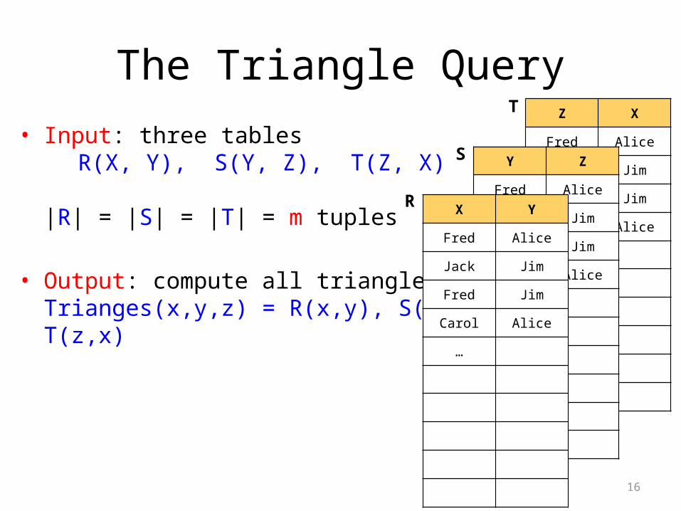
The Triangle Query
• Input: three tablesR(X, Y), S(Y, Z), T(Z, X)
|R| = |S| = |T| = m tuples
• Output: compute all trianglesTrianges(x,y,z) = R(x,y), S(y,z), T(z,x)
Z X
Fred Alice
Jack Jim
Fred Jim
Carol Alice
…
Y Z
Fred Alice
Jack Jim
Fred Jim
Carol Alice
…
X Y
Fred Alice
Jack Jim
Fred Jim
Carol Alice
…
R
S
T

17
Triangles in One Round
• Place servers in a cube p = p1/3 × p1/3 × p1/3
• Each server identified by (i,j,k)
i
j
k
(i,j,k)
p1/3
Server (i,j,k)
Trianges(x,y,z) = R(x,y), S(y,z), T(z,x) |R| = |S| = |T| = m tuples

18
Triangles in One Round
k
(i,j,k)
Z X
Fred Alice
Jack Jim
Fred Jim
Carol Alice
…
Jack JimY Z
Fred Alice
Jack Jim
Fred Jim
Carol Alice
Jim JackJim Jack
X Y
Fred Alice
Jack Jim
Fred Jim
Carol Alice
…
R
S
T
i = h2(Fred)
j = h1(Jim)
Fred JimFred Jim
Fred JimFred Jim
Jim Jack
Jim Jack
Fred JimJim Jack
Jim Jack
Fred Jim
Fred Jim
Jack JimJack Jim
Round 1:Send R(x,y) to all servers (h1(x),h2(y),*)Send S(y,z) to all servers (*, h2(y), h3(z))Send T(z,x) to all servers (h1(x), *, h3(z))
Output:compute locally R(x,y) S(y,z) T(z,x)⋈ ⋈
p1/3
Trianges(x,y,z) = R(x,y), S(y,z), T(z,x) |R| = |S| = |T| = m tuples

19
Communication load per server
Theorem If the data has “no skew”, thenthe HyperCube computes Triangles in one roundwith communication load/server O(m/p2/3) w.h.p.
Theorem Any 1-round algo. has L = Ω(m/p2/3 )
Sub-linear speedupCan we compute Triangles with L = m/p?
Trianges(x,y,z) = R(x,y), S(y,z), T(z,x) |R| = |S| = |T| = m tuples
No!

20
1.1M triples of Twitter data 220k triangles; p=64
2 roundshash-join
1 roundbroadcast 1 round
hypercube
local 1 or 2-step hash-join; local 1-step Leapfrog Trie-join (a.k.a. Generic-Join)
Trianges(x,y,z) = R(x,y), S(y,z), T(z,x) |R| = |S| = |T| = 1.1M

1.1M triples of Twitter data 220k triangles; p=64
Trianges(x,y,z) = R(x,y), S(y,z), T(z,x) |R| = |S| = |T| = 1.1M

HperCube Algorithm for Full CQ
• Write: p = p1 * p2 * … * pk
• Round 1: send Sj(xj1, xj2, …) to all servers whose coordinates agree with
hj1(xj1), hj2(xj2), …
• Output: compute Q locally
pi = the “share” of the variable xi
h1, …, hk =independent
randomfunctions

23
Computing Shares p1, p2, …, pk
Minimize Σj Lj[Afrati’10] nonlinear opt:
Minimize maxj Lj[Beame’13] linear opt:
Load/server from Sj : Lj = m / (pj1 * pj2 * … )
Optimization problem: find p1 * p2 * … * pk = p
Suppose all relations have the same size m

24
Fractional Vertex Cover
Hyper-graph: nodes x1, x2 …, hyper-edges S1, S2, …
• Vertex cover: a set of nodes that includes at least one node from each hyper-edge Sj
• Fractional vertex cover: v1, v2, … vk ≥ 0 s.t.:
• Fractional vertex cover value τ* = minv1,… vk Σi vi

Computing Shares p1, p2, …, pk
Theorem. Optimal shares are: pi = p vi* / τ*
Optimal load per server is: L = m / p1/τ*
1/p1/τ* = speedup
v1*, v2*, …, vk* = optimal fractional vertex cover
Can we do better? No:
Suppose all relations have the same size m
Theorem L = m / p1/τ* is also a lower bound.

26
Examples
t* = 2Triangles(x,y,z) = R(x,y), S(y,z), T(z,x)
L = m / p1/τ*
5-cycle: R(x,y), S(y,z), T(z,u), K(u,v), L(v,x) τ* = 5/2½
½
½
½
Integralvertexcover
τ* = 3/2
½
½½
Fractionalvertexcover

27
Lessons So Far
• MPC model: cost = communication load + rounds
• HyperCube: rounds=1, L = m/p1/τ* Sub-linear speedupNote: it only shuffles data! Still need to compute Q locally.
• Strong optimality guarantee: any algorithm with better load m/ps reports only 1/ps×τ*-1 fraction of answers.
Parallelism gets harder as p increases!
• Total communication = p×L = m × p1-1/τ*
MapReduce model is wrong! It encourages many reducers p

28
Outline
• The MPC Model
• The Algorithm
• Skew matters
• Statistics matter
• Extensions and Open Problems
29
Skew Matters
• If the database is skewed, the query becomes provably harder. We want to optimize for the common case (skew-free) and treat skew separately
• This is different from sequential query processing, were worst-case optimal algorithms (LFTJ, generic-join) are for arbitrary instances, skewed or not.

30
Skew Matters
• Join(x,y,z) = R(x,y),S(y,z)
L = m/p
• Suppose R, S are skewed, e.g. single value y
• The query becomes a cartesian product! Product(x,z) = R(x),S(z)
L = m/p1/2
τ* = 1
0 01
τ* = 2
1 1
Lets examine skew…

31
All You Need to Know About Skew
Hash-partition a bag of m data values to p bins
Fact 1 Expected size of any one fixed bin is m/p
Fact 2 Say that database is skewed if some value has degree > m/p. Then some bin has load > m/p
Fact 3 Conversely, if the database is skew-freethen max size of all bins = O(m/p) w.h.p.
Join: if degree < ∀ m/p then L = O(m/p) w.h.pTriangles: if degree < ∀ m/p1/3 then L = O(m/p2/3
) w.h.p
Hiding log p factors

32
The AGM InequalityAtserias, Grohe, Marx’13
Suppose all relations have the same size m
Theorem. [AGM] Let u1, u2, …, ul be an optimalfractional edge cover, and ρ* = u1+u2+ … +ul Then: |Q| ≤ mρ*

33
The AGM Inequality
Suppose all relations have the same size m
Fact. Any MPC algorithm using r roundsand load/server L satisfies r×L ≥ m / p1/ρ*
Proof.• Tightness of AGM: there exists db s.t. |Q| = mρ*
• AGM: one server reports only (r×L)ρ* answers• All p servers report only p×(r×L)ρ* answers
WAIT: we computed Join with L = m / p now we say L ≥ m / p1/2 ?

34
Lessons so Far
• Skew affects communication dramatically– w/o skew: L = m / p1/τ* fractional vertex cover– w/ skew: L ≥ m / p1/ρ* fractional edge cover
• E.g. Join from linear m/p to m/p1/2
• Focus on skew-free databases.Handle skewed values as a residual query.
35
Outline
• The MPC Model
• The Algorithm
• Skew matters
• Statistics matter
• Extensions and Open Problems

36
Statistics
• So far: all relations have same size m
• In reality, we know their sizes = m1, m2, …
Q1: What is the optimal choice of shares?
Q2: What is the optimal load L?
Will answer Q2, giving closed formula for L. Will answer Q1 indirectly, by showing that HyperCube takes advantage of statistics.

Statistics for Cartesian Product
S1(x)
S2(y
)
2-way product Q(x,y) = S1(x) × S2(y) |S1|=m1, |S2| = m2
Shares p = p1 × p2
L = max(m1 / p1 , m2 / p2)Minimized when m1 / p1 = m2 / p2
t-way product: Q(x1,…,xu) = S1(x1)× …×St(xt):

Fractional Edge Packing
Hyper-graph: nodes x1, x2 …, hyper-edges S1, S2, …
• Edge packing: a set of hyperedges Sj1, Sj2, …, Sjt that are pairwise disjoint (no common nodes)
• Fractional edge packing: u1, u2, … ul ≥ 0 s.t.:
• This is the dual of a fractional vertex cover v1, v2, …, vk
• By duality: maxu1,… ul Σj uj = minv1,, …, vk Σi vi = τ*
39
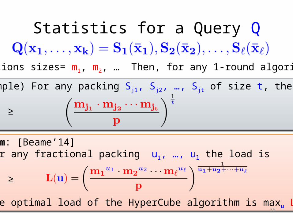
Statistics for a Query Q
Relations sizes= m1, m2, … Then, for any 1-round algorithm
Fact (simple) For any packing Sj1, Sj2, …, Sjt of size t, the load is:
L ≥
Theorem: [Beame’14] (1) For any fractional packing u1, …, ul the load is
L ≥
(2) The optimal load of the HyperCube algorithm is maxu L(u)
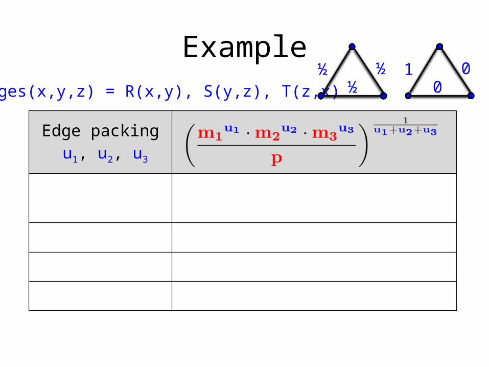
Example
Edge packing u1, u2, u3
1/2, 1/2, 1/2 (m1 m2 m3)1/3 / p2/3
1, 0, 0 m1 / p
0, 1, 0 m2 / p
0, 0, 1 m3 / p
Trianges(x,y,z) = R(x,y), S(y,z), T(z,x)0
01½
½½

Example
Edge packing u1, u2, u3
1/2, 1/2, 1/2 (m1 m2 m3)1/3 / p2/3
1, 0, 0 m1 / p
0, 1, 0 m2 / p
0, 0, 1 m3 / p
Trianges(x,y,z) = R(x,y), S(y,z), T(z,x)0
01½
½½

Example
Edge packing u1, u2, u3
1/2, 1/2, 1/2 (m1 m2 m3)1/3 / p2/3
1, 0, 0 m1 / p
0, 1, 0 m2 / p
0, 0, 1 m3 / p
Trianges(x,y,z) = R(x,y), S(y,z), T(z,x)0
01½
½½

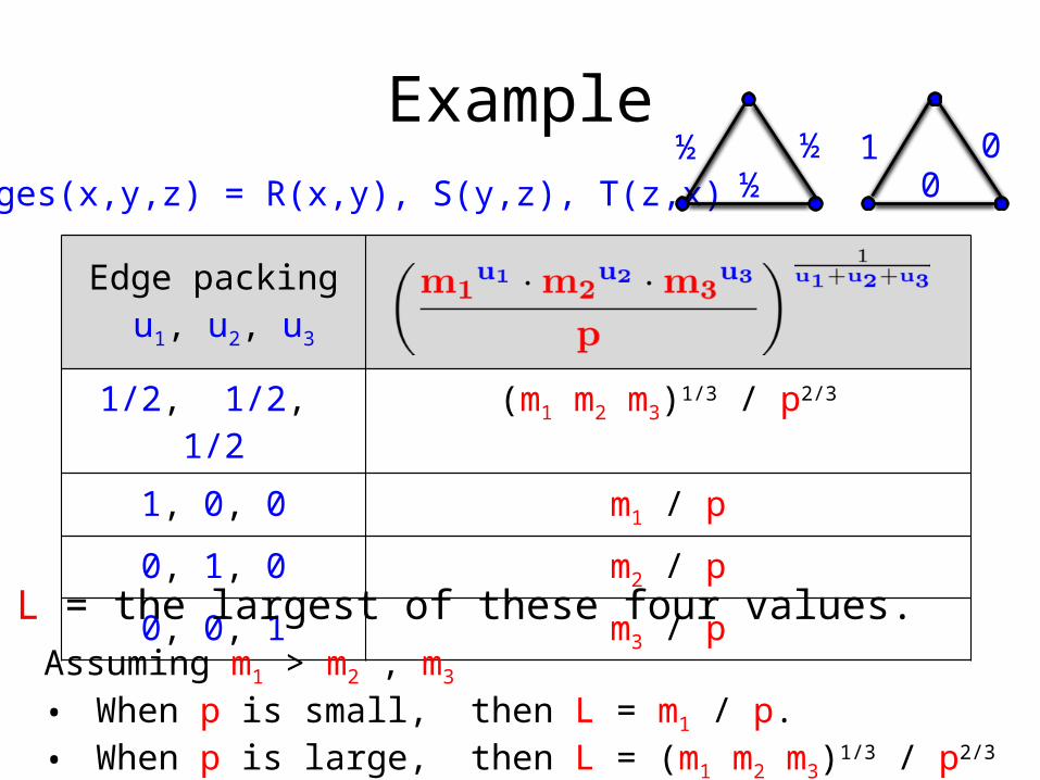
Example
Edge packing u1, u2, u3
1/2, 1/2, 1/2 (m1 m2 m3)1/3 / p2/3
1, 0, 0 m1 / p
0, 1, 0 m2 / p
0, 0, 1 m3 / p
Trianges(x,y,z) = R(x,y), S(y,z), T(z,x)
L = the largest of these four values.
00
1½½
½
Example
Edge packing u1, u2, u3
1/2, 1/2, 1/2 (m1 m2 m3)1/3 / p2/3
1, 0, 0 m1 / p
0, 1, 0 m2 / p
0, 0, 1 m3 / p
Trianges(x,y,z) = R(x,y), S(y,z), T(z,x)
L = the largest of these four values.
00
1½½
½
Assuming m1 > m2 , m3 • When p is small, then L = m1 / p. • When p is large, then L = (m1 m2 m3)1/3 / p2/3
45
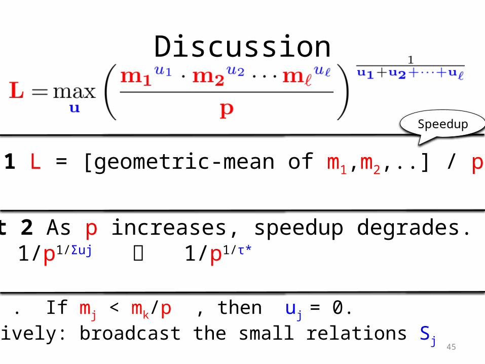
Discussion
Fact 3 . If mj < mk/p , then uj = 0.Intuitively: broadcast the small relations Sj
Fact 1 L = [geometric-mean of m1,m2,..] / p1/Σuj
Speedup
Fact 2 As p increases, speedup degrades. 1/p1/Σuj 1/p1/τ*
46
Outline
• The MPC Model
• The Algorithm
• Skew matters
• Statistics matter
• Extensions and Open Problems

47
Coping with Skew
There are at most O(p) heavy hitters: known by all servers.
HypeSkew algorithm:
1. Run HyperCube on the skew-free part of the database
2. In parallel, for each heavy hitter value c,run HyperSkew on the residual query Q[c/xi](Open problem: how many servers to allocate to c)
Definition A value c is a “heavy hitter” for xi in Sj if degreeSj(xi=c) > mj / pi, where pi = share of xi

48
Coping with Skew
What we know today:• Join(x,y,z) = R(x,y), S(y,z)
Optimal load L: between m/p and m/p1/2
• Triangles(X,Y,Z) = R(X,Y), S(Y,Z), T(Z,X)Optimal load L: between m/p1/3 and m/p1/2
General query Q: still ill understood
Open problem: upper/lower bounds for skewed values

49
Multiple Rounds
What we would like:• Reduce load below m/p1/τ*
– ACQ no-skew: load m/p, rounds O(1) [Afrati’14]– Challenge: large intermediate results
• Reduce the penalty of heavy hitters; – Triangles from m/p1/2 to m/p1/3 in 2 rounds– Challenge: the m/p1/ρ* barrier for skewed data
What else we know today:• Algorithms: [Beame’13,Afrati’14]. Limited.• Upper bound: [Beame’13]. Limited.Open problem: solve multi-rounds

50
More Resources
• Extended slides, exercises, open problems:PhD Open Warsaw, March 2015phdopen.mimuw.edu.pl/index.php?page=l15w1 or search for ‘phd open dan suciu’
• Papers:Beame, Koutris, S, [PODS’13, 14]Chu, Balazinska, S. [SIGMOD’15]
• Myria website: myria.cs.washington.edu/
Thank you!


![ECOMPOSITION CHEMA NORMALIZATIONpages.cs.wisc.edu/~paris/cs564-s18/lectures/lecture-07.pdf · EXAMPLE: INFORMATION LOSS CS 564 [Spring 2018] -Paris Koutris 8 name age phoneNumber](https://static.fdocuments.us/doc/165x107/5ab0784a7f8b9a1d168b5b67/ecomposition-chema-pariscs564-s18lectureslecture-07pdfexample-information-loss.jpg)