Common types of clinical trial design, study objectives ... · Common types of clinical trial...
64
Common types of clinical trial design, study objectives, randomisation and blinding, hypothesis testing, p-values and confidence intervals, sample size calculation David Brown
Transcript of Common types of clinical trial design, study objectives ... · Common types of clinical trial...

Common types of clinical trial design, study objectives, randomisation and blinding, hypothesis testing, p-values and confidence intervals, sample size calculation David Brown

Statistics
• Statistics looks at design and analysis • Our exercise noted an example of a flawed design
(single sample, uncontrolled, biased population selection, regression to the mean)
• And statistical theory can be used to understand the reason for the results
• Not a completely outrageous example

Case study
• Primary endpoint – recurrence rate post-treatment compared with historical rates observed 1-year pre-treatment
• Inclusion criteria include requirement that patient must have been treated for uveitis within the last 3 months

Results
Same problems here Uncontrolled blood pressure trial could be similar – inclusion criteria usually require a high value
Recurrence rates
(n=110) (n=168) pre-implantation (1-year) 68 (62%) 98 (58%) 34 weeks 2 (2%) 8 (5%) 1-year 4 (4%) 11 (7%) 2-years 11 (10%) 28 (17%) 3-years 33 (30%) 80 (48%)

Clinical Trials
• Prospective experiments in medical treatments
• Designed to test a hypothesis about a treatment – Testing of new drugs – Testing old drugs in new indications – Testing of new procedures Comparison of randomised groups

Contrast to Epidemiology
• Clinical trial – Groups differ only by intervention of interest – Patients allocated to treatment, do not choose it
• Epidemiology
– Treatment groups contain confounding factors – e.g. smoking and cancer
• patients have decided to smoke (not been allocated) • smokers tend to drink more coffee • cannot untangle confounding in a trial

Design of Clinical Trials
• Define the question to be answered – New drug better than placebo – New drug plus standard better than standard
alone – New drug better / no worse than a licensed drug
• Patient population • Posology (treatment schedule) • Outcome measure • Define success

Ideal Clinical Trial
• Randomised
• Double-blind
• Controlled (concurrent controls)

Pre-specification
• Everything pre-specified in the protocol
• Analysis pre-specified in the data analysis plan
• Avoids problems of “multiplicity” and “post-hoc” analysis
• There are always problems if people are free to choose anything after the data are unblinded

Controls
• What will the experimental treatment be compared to?
• Placebo control • Active control • Uncontrolled • Historical control
• Concurrent controls are ideal

Problems with uncontrolled trials
• “100 subjects treated, 80 got better, therefore treatment is 80% effective”
• Regression to the mean
• Placebo effect / study effect

Case study Treatment for depression
Drugs with no efficacy can seem impressive in uncontrolled trials
“Active” (n=101)
Placebo (n=102)
Active - Placebo (CI)
p-value
Baseline score 60.7 62.6 Change to Week 8 -22.6 -23.4 +0.8 (-3.1,4.7) p=0.66

Problems with historical controls • “100 subjects treated, 80 got better. This disease
was studied in 1994 and in a sample of 100, 50 got better. So the new treatment is 30% better than the standard”
• Patients may differ May be generally healthier - more time at the
gym • Treatment may differ - doctors more experienced
with the disease • Evaluation may differ - definition of “got better”

Randomisation
• Allocation of subjects to treatment or control • Avoiding bias • Subjective assignment can be biased
– Compassion - sicker patients on active – Enthusiast - Likely responders on treatment
• Systematic (by name, age etc.) can be biased – Lead to imbalance - patients entered based on
treatment allocation • Randomise after patient has been accepted for trial

Simple Randomisation
• A list is generated
• Each row independently randomised – Unpredictable – Could be unbalanced
Blocked Randomisation
• List generated in balanced blocks
• e.g. block size 4 ABBA, BABA • block size 8 ABAAABBA, AAABBBBA
– Small block size - balanced but more predictable – Large block size - less predictable but possible
imbalance

Stratified Randomisation
• Randomise within each strata – e.g. separate list for males and females – e.g. separate lists for older males, younger
males, older females, younger females
• Problematic with large number of important factors • Less necessary in large trials • Not essential for subgroup analyses to be done • Useful if want to ensure balance for a few important
factors

Minimisation / dynamic allocation
• Favours allocation to the group which minimises the imbalance across a range of characteristics e.g. sex, age, country
• Allocate with certainty, or with a probability > 0.5 • Not recommended in guideline • - properties not well understood • - costly mistakes can be made! • Only use if really necessary

Blinding
• Double-blind – Patient and investigator blind
• Single-blind – Patient blind
• Open • Blinded independent review

Why blind? • Avoiding bias • Why blind patients?
– Patients expectations can influence response – Might report more adverse events if known to be on
treatment – Might assume no efficacy if on placebo
• Why blind investigators? – May subconsciously influence outcome measures – Some endpoints controlled by investigators and could be
influenced by knowledge of treatment

How is blinding done?
• Test vs. Placebo – Make placebo identical to active
• Test vs. Active
– Make both treatments identical – OR construct placebo for each (double dummy)

Difficult to blind
• Trials involving surgery – Sham operations present ethical difficulties
• Trials of interventions such as massage or
psychotherapy – Impossible to blind (but can at least make
assessors blind)
Trial design - Parallel Group trials
• Patients are each randomised to ONE of the treatment arms
• The results from the 2 (or more) groups are compared at the end of the trial

Crossover trials
• Patients initially randomised to one of the treatment then “cross-over” to the other treatment
• Washout between treatment periods
• Difference between treatments for each patient considered adjusting for period effect
Crossover trials
Advantages Fewer patients needed Eliminates between patient variability Test is “Within-patient” Disadvantages Carry-over effects possible Can’t be used in curable diseases or for long-term treatment Data wasted when patients drop-out in first period Duration of trial (for each patient) longer

Sample size calculations • Give an approximate idea of the number of patients needed • to give a good chance of detecting the expected effect size • Linked to the analysis (or significance test) that will be
carried out at the end of the trial • The calculation requires:
– Treatment effect of interest – Estimated variability – Desired Power – Required significance level

Sample size calculations
• Sample size can never be “agreed”
• More subjects included – more chance of effect
(if it exists) being detected

Treatment Effect
• A treatment advantage of clinical interest • If the treatment has this effect it is worth developing • Large effect = small sample size
Variance
• General variability of the endpoint being measured • Can reduce variability with good trial design
• Large variance = large sample size

Significance level
• The significance level that the final analysis will be conducted at
• Also known as “Type I error” • Also known as “consumer’s risk” • Also known as “alpha” • The probability that an ineffective treatment will be
declared to be effective • Normally fixed at 0.05 (5%) • Low Type I error = high sample size

Power
• The probability of the study to detect the difference of interest (if the treatment really does have the expected effect)
• Also known as 1 minus the “Type II error” • Type II error is the probability that an effective
treatment will be declared to be ineffective • Type II error also known as “producer’s risk” • Common values for power 80% and 90% • High power = High sample size

Analysis and interpretation
• Hypothesis testing • P-values • Confidence intervals • Interpretation • Replication

How statistics works
• We can’t always measure everyone!
• “Sampling is the selection of individual observations intended to yield some knowledge about a population of concern for the purposes of statistical inference.”
• This gives ‘estimate’ plus associated ‘error’
– When we measure a quantity in a large number of individuals we call the pattern of values obtained a distribution.

• Calculate mean, median, mode, variability and standard deviation:
• 1, 2, 2, 2, 4, 4, 6
• Mean = Mode =
• Median = Variance =
• Standard Deviation =

• Calculate mean, median, mode, variability and standard deviation:
• 1, 2, 2, 2, 4, 4, 6
• Mean = 3 Mode = 2
• Median = 2 Variance = 18/7 or 18/6 • (18 from (-2)2+3×(-1)2+2×12+32) • Standard Deviation = sqrt VAR

The normal distribution
• Symmetrical,
• Mean = Median = Mode
• Mean ± 2 x sd covers most of distribution
• Many examples: height of people, blood pressure…

Central limit theorem
• As sample size increases, the sampling distribution of sample means approaches that of a normal distribution with a mean the same as the population and a standard deviation equal to the standard deviation of the population divided by the square root of n (the sample size).
• Or …the mean of several data values tends to follow a normal distribution, even if the data generating the distribution were non-normal
• Sampling repeatedly leads to a distribution that we can use!
Statistics as PROOF
– Hypothesis testing
– Type I and Type II error
– P-values and confidence intervals

An early hypothesis test
• Sir Ronald Aylmer Fisher (1890-1962) didn’t believe that a particular lady could determine the manner of tea preparation through taste alone, so he arranged an experiment … he lost!

Statistics as PROOF - hypothesis testing
• Null hypothesis (H0) is set a priori • If the trial aims to detect a difference, null hypothesis is that there
is no difference (hence “null”) • e.g. H0: there is no difference between the new treatment
and placebo • i.e. distributions in same place
• The “alternative hypothesis” (H1 or HA) is the hypothesis of interest
• e.g. H1:The new treatment is better than placebo • i.e distribution shift

An example from Fisher
• H0 – The lady can’t determine tea preparation through taste alone
• H1 – She can • n=8 cups of tea - test statistic is number of
correctly identified cups • If 8/8 Fisher was prepared to reject H0. • What are the chances of 8 successes if H0 true? The experiment provided the Lady with 8 randomly ordered cups of tea – 4 prepared by first adding milk, 4 prepared by first adding the tea. She was to select the 4 cups prepared by one method

• Answer: 1/70 (=0.014) – There are 70 ways of selecting 4 items from 8
• If there were 6 cups, 3 with milk first it would be 1/20 = 0.05

Type I and Type II error
Outcome Fail Succeed
True difference Type II error Company risk False accept H0 Power = 1-Type II
Correct!
No true difference Correct! Type I error False reject H0 Regulator’s risk
How can we tell the difference between a true effect and a false effect? We can’t!!

Type I and Type II error
• Type I error is of critical importance to regulators in assessing MAAs and must be maintained
• If nominal significance level set to 5%, Type I error can be said to be 5%
• Actually we are usually only testing in one direction – is drug better than placebo, not is drug different from placebo (i.e. better or worse) – so more accurately the type I error is set to 2.5% one-sided
• Otherwise likelihood of false positive increased
• Type II error less critical for regulatory purposes but not irrelevant – e.g. ethics, safety

1-sided vs. 2-sided inference
• Quote from ICH E9
• “The issue of one-sided or two-sided approaches to inference is controversial and a diversity of views can be found in the statistical literature. The approach of setting type I errors for one-sided tests at half the conventional type I error used in two-sided tests is preferable in regulatory settings. This promotes consistency with the two-sided confidence intervals that are generally appropriate for estimating the possible size of the difference between two treatments.”

P-values • The p-value is the probability of this data (or more extreme) IF H0 IS
TRUE. • Critical value is usually 5% or 0.05 (2.5% 1-sided, or 0.025 1-sided, but
p-values usually reported 2-sided – watch out for this if 1-sided p-values are reported but 0.05 still used as critical value)
• “A had a change from baseline of 3 points, while B achieved only 1 (p=0.005). This means the probability that A is better than B is 99.5%.” WRONG!!!
• P-values should be spelt out in full - not summarised as <, > etc.

P-values
• Null hypothesis: Coin is unbiased
• Alternative hypothesis: Coin is biased
• 20 coin tosses – 14 or more the same. p=11.5% (0.115)
• 20 coin tosses – 15 or more the same. p=4.1% (0.041)

P-values from coin tosses
• 1/1 same = 1.0 • 2/2 same = 0.5 • 3/3 same = 0.25 • 4/4 same = 0.125 • 5/5 same = 0.0625 • 6/6 same = 0.03125 • 7/7 same = 0.015625

Interpreting P-values
• Black and white or shades of grey? • P=0.0501 • P=0.0499 • If P=0.06 trends towards significance • Does P=0.04 trend towards non-significance?
• Easy to interpret P<0.05, what about P>0.05?

Interpreting non-significant P-values
• Which of the sentences below should be concluded from a non-significant P-value? A - Treatment effects are equivalent B - Treatment effects are similar C- No difference between effects of treatments D- No evidence of a difference between effects of
treatments E - Data are inconclusive

Example: Pre-clinical data – Incidence of blindness in mice following
exposure to test low dose or high dose low high total Blind 1 3 10 Not Blind 11 9 14 Totals 12 12 24 – No ‘significant’ difference between doses – Is it appropriate to conclude that high dose does
not increase incidence of blindness?

Interpreting non-significant P-values • Non-significant P-values …
• …DO NOT imply equivalence / similarity
/ comparability or any other synonym.
• … simply mean that the evidence to reject null hypothesis is inadequate. This doesn’t mean that the null hypothesis is true

• “The result, albeit not statistically significant, is certainly clinically relevant”
• A dangerous phrase – the lack of statistical significance means that there is a reasonable chance there is no treatment effect – the point estimate may seem large but we shouldn’t let our head be turned, as we are uncertain about the true value (see confidence intervals later).

Calculating P-values for continuous data
• e.g. t-test (same as one-way ANOVA) • Confidence intervals and hypothesis tests rely on Student's t-distribution to
cope with uncertainty resulting from estimating the standard deviation from a sample, whereas if the population standard deviation were known, a normal distribution would be used.

Calculating P-values
• Test: 75, 68, 71, 75, 66, 70, 68, 68 • Mean = 70.125, Var 11.27, n(test)=8
• Control: 58, 56, 61, 60, 62, 60, 59, 68
• Mean = 53.77, Var 11.27, n(control)=8
– Signal = 70.125 – 53.77 = 16.35 – Noise = 2.903 – T = 5.63
– Degrees of freedom = N-2 = 14
– P = 0.00006

Statistics as PROOF - Confidence intervals • Definition 1: If this experiment were repeated 100 times, the
truth would be expected to be in the 95% confidence interval 95 times.
• Definition 2: A confidence interval shows the range of plausible values for the difference between treatments
• At the centre is the “point estimate” • The difference seen in the trial • e.g. mean or lsmean difference
• The two extremes are the “lower bound” and the “upper bound”

Statistics as PROOF - Confidence intervals
– For ‘differences’ (A-B) if the lower bound of a 95% confidence interval is above zero (or the upper bound below zero), statistical significance has been achieved at the 0.05 level
– For ‘ratios’ (A/B) if the lower bound of a 95% confidence interval is above one (or the upper bound below one), statistical significance has been achieved at the 0.05 level

Calculating confidence intervals • The standard error of a sample statistic (such as sample mean) shows
how precisely it has been estimated. • As the sample size increases we have a better estimate so the standard
error is smaller • It is also small if there little variability in the general population • Standard error = sd / sqrt(n) • If the data are assumed to be normally distributed, the following
expressions can be used to calculate the upper and lower 95% confidence limits, where 'x' is equal to the sample mean, 'y' is equal to the standard error of the sample, and 1.96 is the .975 quantile of the normal distribution.
• Upper 95% limit=x +(y*1.96) • Lower 95% limit=x - (y*1.96). • In practice we use the t distribution (rather than 1.96 from the
normal) unless the sample size is large
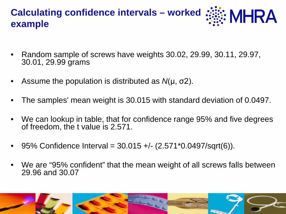
Calculating confidence intervals – worked example
• Random sample of screws have weights 30.02, 29.99, 30.11, 29.97, 30.01, 29.99 grams
• Assume the population is distributed as N(μ, σ2).
• The samples' mean weight is 30.015 with standard deviation of 0.0497. • We can lookup in table, that for confidence range 95% and five degrees
of freedom, the t value is 2.571.
• 95% Confidence Interval = 30.015 +/- (2.571*0.0497/sqrt(6)).
• We are “95% confident” that the mean weight of all screws falls between 29.96 and 30.07

Calculating confidence intervals – worked example
• If we were interested in whether the true mean was above 29.9 (Ho: mean =29.9) we would have p<0.05.
• If we needed to be confident the mean was above 30 (Ho: mean =30) we would have p>0.05.

Confidence intervals
• 20 objects tested • 18 successes • Success percentage = 90% • 95% CI – (68.3%, 98.77%) • If we wanted to test whether the true success rate
was above 65% (Ho: success rate = 0.65) we would have p<0.05
• If we were testing Ho: success rate =0.70 we have p>0.05. Can’t rule out 70%.
• 36/40 successes – (76.34%, 97.21%)

Size of difference • Statistical significance alone can be said to have little meaning –
need to know size of difference in addition to whether effect is ‘real’.
• We talk of (clinical) relevance
• Statistical significance AND clinical relevance required for a product license
• Judged in context of “risk -benefit” evaluation
• Looking at confidence intervals more informative than only looking at p-values

Value of replication
• Findings more convincing if replicated • Generally 2 pivotal trials looked for • Single pivotal trial guideline
– Includes recommendation for more extreme statistical evidence than p<0.05
• For a single trial to provide the same statistical evidence as 2 trials positive at 2-side p<0.05, it would need to achieve 2-sided p<0.00125
• People sometimes suggest 0.01 – this does not come close to replicating 2 trials

Value of replication
• Even with this extreme value single trial does not have the other benefits of true replication
• e.g replicated in different centres shows it was not just a finding that only arises because of something specific about those centres
• Coin toss experiment more convincing if different person does the tossing and replicates results than if I just do it again
• Increases generalisability.