Application Note

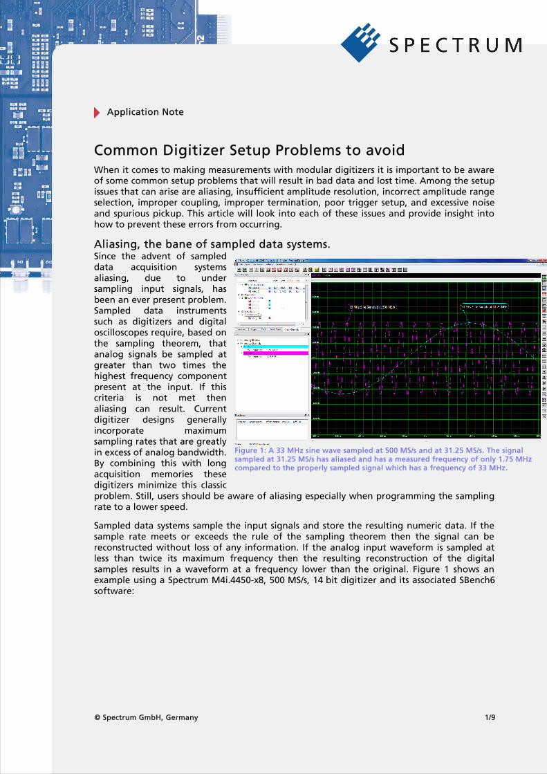
Common Digitizer Setup Problems to avoidWhen it comes to making measurements with modular digitizers it is important to be aware of some common setup problems that will result in bad data and lost time. Among the setup issues that can arise are aliasing, insufficient amplitude resolution, incorrect amplitude range selection, improper coupling, improper termination, poor trigger setup, and excessive noise and spurious pickup. This article will look into each of these issues and provide insight into how to prevent these errors from occurring.

Aliasing, the bane of sampled data systems.Since the advent of sampled data acquisition systems aliasing, due to under sampling input signals, has been an ever present problem. Sampled data instruments such as digitizers and digital oscilloscopes require, based on the sampling theorem, that analog signals be sampled at greater than two times the highest frequency component present at the input. If this criteria is not met then aliasing can result. Current digitizer designs generally incorporate maximum sampling rates that are greatly in excess of analog bandwidth. By combining this with long acquisition memories these digitizers minimize this classic problem. Still, users should be aware of aliasing especially when programming the sampling rate to a lower speed.

Sampled data systems sample the input signals and store the resulting numeric data. If the sample rate meets or exceeds the rule of the sampling theorem then the signal can be reconstructed without loss of any information. If the analog input waveform is sampled at less than twice its maximum frequency then the resulting reconstruction of the digital samples results in a waveform at a frequency lower than the original. Figure 1 shows an example using a Spectrum M4i.4450-x8, 500 MS/s, 14 bit digitizer and its associated SBench6 software:

© Spectrum GmbH, Germany 1/9

Figure 1: A 33 MHz sine wave sampled at 500 MS/s and at 31.25 MS/s. The signal sampled at 31.25 MS/s has aliased and has a measured frequency of only 1.75 MHz compared to the properly sampled signal which has a frequency of 33 MHz.

Application Note

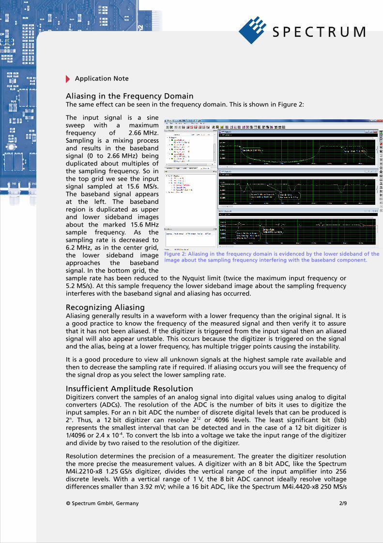
Aliasing in the Frequency DomainThe same effect can be seen in the frequency domain. This is shown in Figure 2:

The input signal is a sine sweep with a maximum frequency of 2.66 MHz. Sampling is a mixing process and results in the baseband signal (0 to 2.66 MHz) being duplicated about multiples of the sampling frequency. So in the top grid we see the input signal sampled at 15.6 MS/s. The baseband signal appears at the left. The baseband region is duplicated as upper and lower sideband images about the marked 15.6 MHz sample frequency. As the sampling rate is decreased to 6.2 MHz, as in the center grid, the lower sideband image approaches the baseband signal. In the bottom grid, the sample rate has been reduced to the Nyquist limit (twice the maximum input frequency or 5.2 MS/s). At this sample frequency the lower sideband image about the sampling frequency interferes with the baseband signal and aliasing has occurred.

Recognizing AliasingAliasing generally results in a waveform with a lower frequency than the original signal. It is a good practice to know the frequency of the measured signal and then verify it to assure that it has not been aliased. If the digitizer is triggered from the input signal then an aliased signal will also appear unstable. This occurs because the digitizer is triggered on the signal and the alias, being at a lower frequency, has multiple trigger points causing the instability.

It is a good procedure to view all unknown signals at the highest sample rate available and then to decrease the sampling rate if required. If aliasing occurs you will see the frequency of the signal drop as you select the lower sampling rate.

Insufficient Amplitude ResolutionDigitizers convert the samples of an analog signal into digital values using analog to digital converters (ADCs). The resolution of the ADC is the number of bits it uses to digitize the input samples. For an n bit ADC the number of discrete digital levels that can be produced is 2n. Thus, a 12 bit digitizer can resolve 212 or 4096 levels. The least significant bit (lsb) represents the smallest interval that can be detected and in the case of a 12 bit digitizer is 1/4096 or 2.4 x 10-4. To convert the lsb into a voltage we take the input range of the digitizer and divide by two raised to the resolution of the digitizer.

Resolution determines the precision of a measurement. The greater the digitizer resolution the more precise the measurement values. A digitizer with an 8 bit ADC, like the Spectrum M4i.2210-x8 1.25 GS/s digitizer, divides the vertical range of the input amplifier into 256 discrete levels. With a vertical range of 1 V, the 8 bit ADC cannot ideally resolve voltage differences smaller than 3.92 mV; while a 16 bit ADC, like the Spectrum M4i.4420-x8 250 MS/s

© Spectrum GmbH, Germany 2/9

Figure 2: Aliasing in the frequency domain is evidenced by the lower sideband of the image about the sampling frequency interfering with the baseband component.

Application Note

digitizer with 65656 discrete levels, can ideally resolve voltage differences as small as 15 µV.

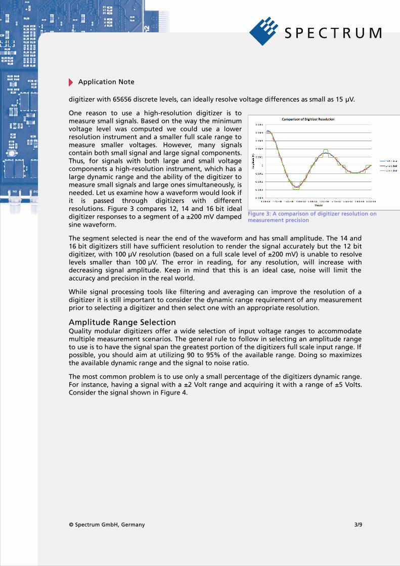
One reason to use a high-resolution digitizer is to measure small signals. Based on the way the minimum voltage level was computed we could use a lower resolution instrument and a smaller full scale range to measure smaller voltages. However, many signals contain both small signal and large signal components. Thus, for signals with both large and small voltage components a high-resolution instrument, which has a large dynamic range and the ability of the digitizer to measure small signals and large ones simultaneously, is needed. Let us examine how a waveform would look if it is passed through digitizers with different resolutions. Figure 3 compares 12, 14 and 16 bit ideal digitizer responses to a segment of a ±200 mV damped sine waveform.

The segment selected is near the end of the waveform and has small amplitude. The 14 and 16 bit digitizers still have sufficient resolution to render the signal accurately but the 12 bit digitizer, with 100 µV resolution (based on a full scale level of ±200 mV) is unable to resolve levels smaller than 100 µV. The error in reading, for any resolution, will increase with decreasing signal amplitude. Keep in mind that this is an ideal case, noise will limit the accuracy and precision in the real world.

While signal processing tools like filtering and averaging can improve the resolution of a digitizer it is still important to consider the dynamic range requirement of any measurement prior to selecting a digitizer and then select one with an appropriate resolution.

Amplitude Range SelectionQuality modular digitizers offer a wide selection of input voltage ranges to accommodate multiple measurement scenarios. The general rule to follow in selecting an amplitude range to use is to have the signal span the greatest portion of the digitizers full scale input range. If possible, you should aim at utilizing 90 to 95% of the available range. Doing so maximizes the available dynamic range and the signal to noise ratio.

The most common problem is to use only a small percentage of the digitizers dynamic range. For instance, having a signal with a ±2 Volt range and acquiring it with a range of ±5 Volts. Consider the signal shown in Figure 4.

© Spectrum GmbH, Germany 3/9

Figure 3: A comparison of digitizer resolution on measurement precision

Application Note

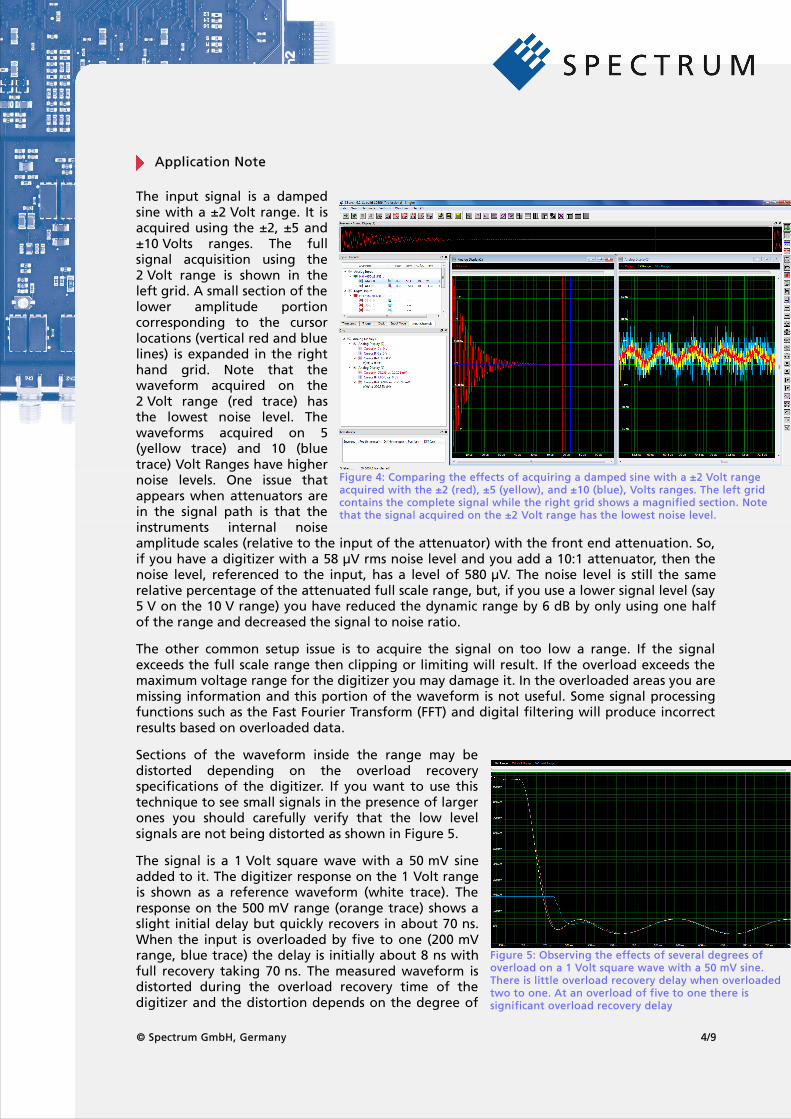
The input signal is a damped sine with a ±2 Volt range. It is acquired using the ±2, ±5 and ±10 Volts ranges. The full signal acquisition using the 2 Volt range is shown in the left grid. A small section of the lower amplitude portion corresponding to the cursor locations (vertical red and blue lines) is expanded in the right hand grid. Note that the waveform acquired on the 2 Volt range (red trace) has the lowest noise level. The waveforms acquired on 5 (yellow trace) and 10 (blue trace) Volt Ranges have higher noise levels. One issue that appears when attenuators are in the signal path is that the instruments internal noise amplitude scales (relative to the input of the attenuator) with the front end attenuation. So, if you have a digitizer with a 58 µV rms noise level and you add a 10:1 attenuator, then the noise level, referenced to the input, has a level of 580 µV. The noise level is still the same relative percentage of the attenuated full scale range, but, if you use a lower signal level (say 5 V on the 10 V range) you have reduced the dynamic range by 6 dB by only using one half of the range and decreased the signal to noise ratio.

The other common setup issue is to acquire the signal on too low a range. If the signal exceeds the full scale range then clipping or limiting will result. If the overload exceeds the maximum voltage range for the digitizer you may damage it. In the overloaded areas you are missing information and this portion of the waveform is not useful. Some signal processing functions such as the Fast Fourier Transform (FFT) and digital filtering will produce incorrect results based on overloaded data.

Sections of the waveform inside the range may be distorted depending on the overload recovery specifications of the digitizer. If you want to use this technique to see small signals in the presence of larger ones you should carefully verify that the low level signals are not being distorted as shown in Figure 5.

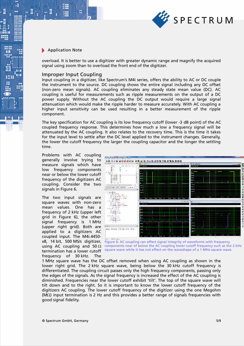
The signal is a 1 Volt square wave with a 50 mV sine added to it. The digitizer response on the 1 Volt range is shown as a reference waveform (white trace). The response on the 500 mV range (orange trace) shows a slight initial delay but quickly recovers in about 70 ns. When the input is overloaded by five to one (200 mV range, blue trace) the delay is initially about 8 ns with full recovery taking 70 ns. The measured waveform is distorted during the overload recovery time of the digitizer and the distortion depends on the degree of

© Spectrum GmbH, Germany 4/9

Figure 4: Comparing the effects of acquiring a damped sine with a ±2 Volt range acquired with the ±2 (red), ±5 (yellow), and ±10 (blue), Volts ranges. The left grid contains the complete signal while the right grid shows a magnified section. Note that the signal acquired on the ±2 Volt range has the lowest noise level.

Figure 5: Observing the effects of several degrees of overload on a 1 Volt square wave with a 50 mV sine. There is little overload recovery delay when overloaded two to one. At an overload of five to one there is significant overload recovery delay

Application Note

overload. It is better to use a digitizer with greater dynamic range and magnify the acquired signal using zoom than to overload the front end of the digitizer.

Improper Input CouplingInput coupling in a digitizer, like Spectrum’s M4i series, offers the ability to AC or DC couple the instrument to the source. DC coupling shows the entire signal including any DC offset (non-zero mean signals). AC coupling eliminates any steady state mean value (DC). AC coupling is useful for measurements such as ripple measurements on the output of a DC power supply. Without the AC coupling the DC output would require a large signal attenuation which would make the ripple harder to measure accurately. With AC coupling a higher input sensitivity can be used resulting in a better measurement of the ripple component.

The key specification for AC coupling is its low frequency cutoff (lower -3 dB point) of the AC coupled frequency response. This determines how much a low a frequency signal will be attenuated by the AC coupling. It also relates to the recovery time. This is the time it takes for the input level to settle after the DC level applied to the instrument changes. Generally, the lower the cutoff frequency the larger the coupling capacitor and the longer the settling time.

Problems with AC coupling generally involve trying to measure signals which have low frequency components near or below the lower cutoff frequency of the digitizers AC coupling. Consider the two signals in Figure 6.

The two input signals are square waves with non-zero mean values. One has a frequency of 2 kHz (upper left grid in Figure 6), the other signal frequency is 1 MHz (upper right grid). Both are applied to a digitizers AC coupled input. The M4i.4450-x8, 14 bit, 500 MS/s digitizer, using AC coupling and 50 termination has a lower cutoff frequency of 30 kHz. The 1 MHz square wave has the DC offset removed when using AC coupling as shown in the lower right grid. The 2 kHz square wave, being below the 30 kHz cutoff frequency is differentiated. The coupling circuit passes only the high frequency components, passing only the edges of the signals. As the signal frequency is increased the effect of the AC coupling is diminished. Frequencies near the lower cutoff exhibit ‘tilt’. The top of the square wave will tilt down and to the right. So it is important to know the lower cutoff frequency of the digitizers AC coupling. The lower cutoff frequency of the digitizer using the one Megohm (M ) input termination is 2 Hz and this provides a better range of signals frequencies with good signal fidelity.

© Spectrum GmbH, Germany 5/9

Figure 6: AC coupling can affect signal integrity of waveforms with frequency components near of below the AC coupling lower cutoff frequency such as the 2 kHz square wave while it has not effect on the waveshape of a 1 MHz square wave.

Application Note

Improper TerminationA measuring instrument should terminate the source properly. For most radio frequency (RF) measurements this is generally a 50 termination. A matching termination minimizes signal losses due to reflections. The figures of merit for the 50 matching are return loss or voltage standing wave ratio (VSWR). Either of these figures of merit indicate the quality of the impedance match.

If the source device has a high output impedance then it is more properly matched with a 1 M high impedance termination which minimizes circuit loading. The 1 M termination also allows the use of high impedance oscilloscope probes which further increase the load impedance.

Impedance matching to other standard terminations, like 75 for video or 600 for audio, can be accomplished by using a 1 M termination combined with a suitable external termination.

Choosing an incorrect termination can cause some interesting effects as shown in Figure 7:

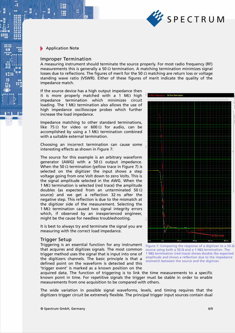
The source for this example is an arbitrary waveform generator (AWG) with a 50 output impedance. When the 50 termination (yellow trace in Figure 7) is selected on the digitizer the input shows a step voltage going from one Volt down to zero Volts. This is the signal amplitude selected in the AWG. When the 1 M termination is selected (red trace) the amplitude doubles (as expected from an unterminated 50 source) and we get a reflection 32 ns after the negative step. This reflection is due to the mismatch at the digitizer side of the measurement. Selecting the 1 M termination caused two signal integrity errors which, if observed by an inexperienced engineer, might be the cause for needless troubleshooting.

It is best to always try and terminate the signal you are measuring with the correct load impedance.

Trigger SetupTriggering is an essential function for any instrument that acquires and digitizes signals. The most common trigger method uses the signal that is input into one of the digitizers channels. The basic principle is that a defined point on the waveform is detected and this ‘trigger event’ is marked as a known position on the acquired data. The function of triggering is to link the time measurements to a specific known point in time. For repetitive signals the trigger must be stable in order to enable measurements from one acquisition to be compared with others.

The wide variation in possible signal waveforms, levels, and timing requires that the digitizers trigger circuit be extremely flexible. The principal trigger input sources contain dual

© Spectrum GmbH, Germany 6/9

Figure 7: Comparing the response of a digitizer to a 50 source using both a 50 and a 1 M termination. The 1 M termination (red trace) shows double the expected amplitude and shows a reflection due to the impedance mismatch between the source and the digitizer.

Application Note

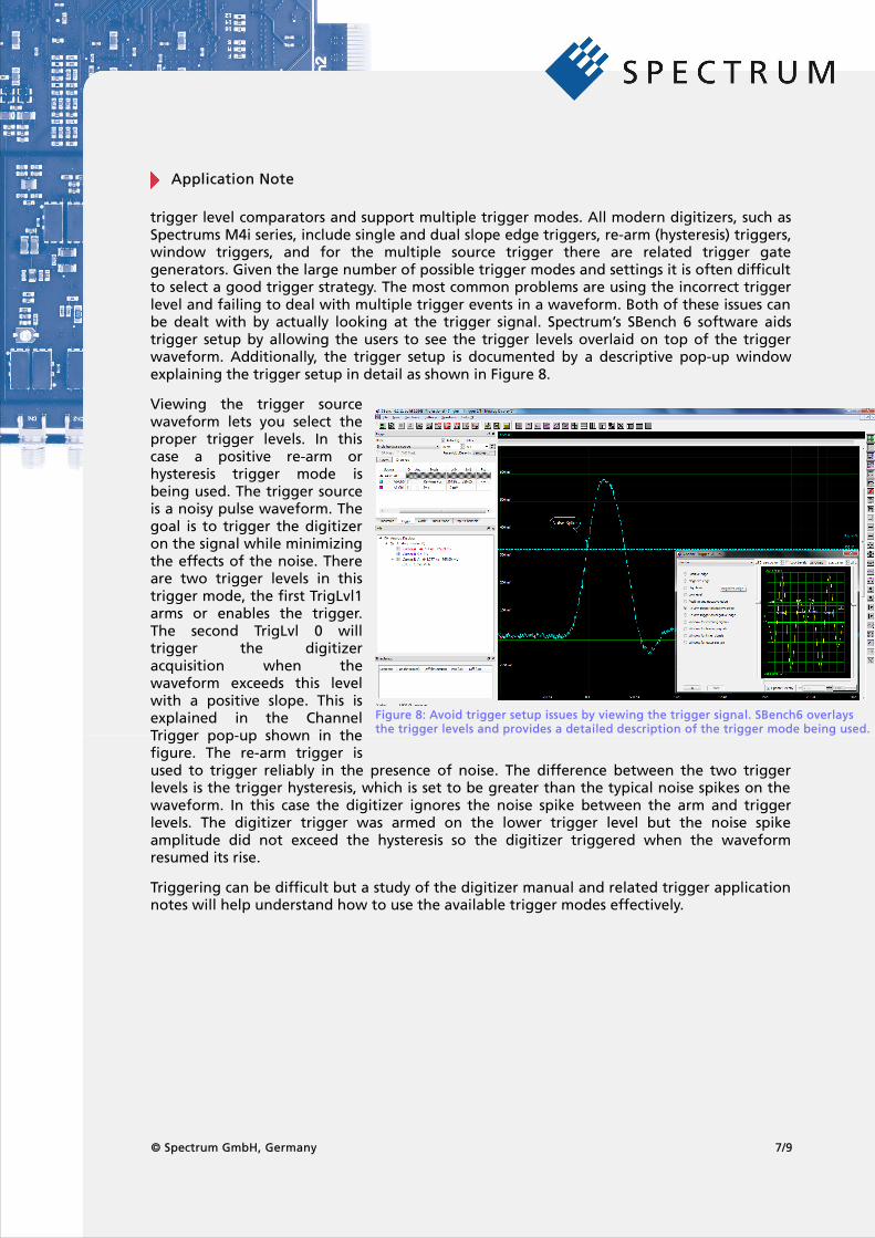
trigger level comparators and support multiple trigger modes. All modern digitizers, such as Spectrums M4i series, include single and dual slope edge triggers, re-arm (hysteresis) triggers, window triggers, and for the multiple source trigger there are related trigger gate generators. Given the large number of possible trigger modes and settings it is often difficult to select a good trigger strategy. The most common problems are using the incorrect trigger level and failing to deal with multiple trigger events in a waveform. Both of these issues can be dealt with by actually looking at the trigger signal. Spectrum’s SBench 6 software aids trigger setup by allowing the users to see the trigger levels overlaid on top of the trigger waveform. Additionally, the trigger setup is documented by a descriptive pop-up window explaining the trigger setup in detail as shown in Figure 8.

Viewing the trigger source waveform lets you select the proper trigger levels. In this case a positive re-arm or hysteresis trigger mode is being used. The trigger source is a noisy pulse waveform. The goal is to trigger the digitizer on the signal while minimizing the effects of the noise. There are two trigger levels in this trigger mode, the first TrigLvl1 arms or enables the trigger. The second TrigLvl 0 will trigger the digitizer acquisition when the waveform exceeds this level with a positive slope. This is explained in the Channel Trigger pop-up shown in the figure. The re-arm trigger is used to trigger reliably in the presence of noise. The difference between the two trigger levels is the trigger hysteresis, which is set to be greater than the typical noise spikes on the waveform. In this case the digitizer ignores the noise spike between the arm and trigger levels. The digitizer trigger was armed on the lower trigger level but the noise spike amplitude did not exceed the hysteresis so the digitizer triggered when the waveform resumed its rise.

Triggering can be difficult but a study of the digitizer manual and related trigger application notes will help understand how to use the available trigger modes effectively.

© Spectrum GmbH, Germany 7/9

Figure 8: Avoid trigger setup issues by viewing the trigger signal. SBench6 overlays the trigger levels and provides a detailed description of the trigger mode being used.

Application Note

Noise and InterferenceHigh resolution modular digitizers are designed to minimize internal noise and, because of their large dynamic range, it is important to make sure that extraneous noise and interfering signals do not contaminate the measurements made with them. Interfering signals can be coupled into measurements via either conducted or radiated signal paths.

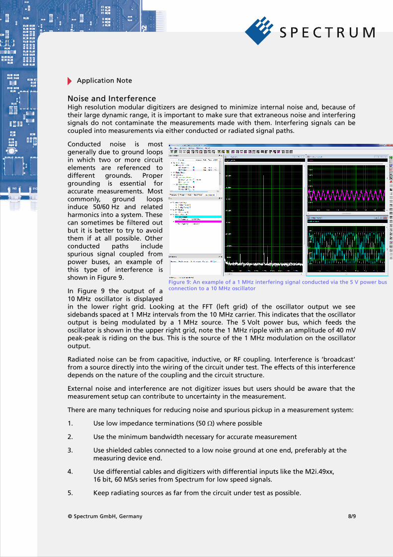
Conducted noise is most generally due to ground loops in which two or more circuit elements are referenced to different grounds. Proper grounding is essential for accurate measurements. Most commonly, ground loops induce 50/60 Hz and related harmonics into a system. These can sometimes be filtered out but it is better to try to avoid them if at all possible. Other conducted paths include spurious signal coupled from power buses, an example of this type of interference is shown in Figure 9.

In Figure 9 the output of a 10 MHz oscillator is displayed in the lower right grid. Looking at the FFT (left grid) of the oscillator output we see sidebands spaced at 1 MHz intervals from the 10 MHz carrier. This indicates that the oscillator output is being modulated by a 1 MHz source. The 5 Volt power bus, which feeds the oscillator is shown in the upper right grid, note the 1 MHz ripple with an amplitude of 40 mV peak-peak is riding on the bus. This is the source of the 1 MHz modulation on the oscillator output.

Radiated noise can be from capacitive, inductive, or RF coupling. Interference is ‘broadcast’ from a source directly into the wiring of the circuit under test. The effects of this interference depends on the nature of the coupling and the circuit structure.

External noise and interference are not digitizer issues but users should be aware that the measurement setup can contribute to uncertainty in the measurement.

There are many techniques for reducing noise and spurious pickup in a measurement system:

1. Use low impedance terminations (50 ) where possible

2. Use the minimum bandwidth necessary for accurate measurement

3. Use shielded cables connected to a low noise ground at one end, preferably at the measuring device end.

4. Use differential cables and digitizers with differential inputs like the M2i.49xx, 16 bit, 60 MS/s series from Spectrum for low speed signals.

5. Keep radiating sources as far from the circuit under test as possible.

© Spectrum GmbH, Germany 8/9

Figure 9: An example of a 1 MHz interfering signal conducted via the 5 V power bus connection to a 10 MHz oscillator

Application Note

6. If possible use magnetic shielding to reduce inductive pickup near motors and other electromagnetic devices.

7. Ground all measuring instruments to a common, low noise ground

8. Use high quality, low loss cables.

9. Secure cables so that they cannot move or vibrate to reduce ‘triboelectric’ generation.

10. Properly filter all power connections in the circuit under test.

ConclusionThis article reviewed some of the more common sources of error in modular digitizer based measurement systems. Consult the websites of digitizer manufacturers and read through their application notes and case histories to learn more about applying digitizers more effectively. There are other sources of error and experience with measurements is, perhaps, the best teacher.

Authors:Arthur Pini Independent ConsultantGreg Tate Asian Business Manager, Spectrum GmbHOliver Rovini Technical Manager, Spectrum GmbH

© Spectrum GmbH, Germany 9/9