comments on Draft Plan Bay Area 2050: rising groundwater impacts on PDA's, andunjust air pollution exposure in East Oakland

Kristina Hill < >Thu 7/1/2021 12:31 PMTo: info@planbayarea.org <info@planbayarea.org>; EIR Comments <eircomments@bayareametro.gov>

1 attachments (5 MB)Plane Hill May 2019 Groundwater and Sea Level Rise in the SF Bay Area.pdf;

*External Email*

Dear Colleagues,

I write as a fellow planner, for two reasons: first, I want to compliment you on your efforts to create a regional plan,which is critical to the region's future. Second, I ask you to reconsider two big issues that the Plan has notaddressed. Those are (A) rising groundwater within a mile or more of the shore, and (B) unequal air qualityimpacts in Oakland that are sustained by the ban on trucks for Interstate 580.

A. Rising seas and rising groundwater

Unfortunately, as sea levels rise, unconfined shallow coastal groundwater will also rise. Please see our attached peer-reviewed paper for a map of likely impact zones in the Bay Area. This will create new impacts on building foundations,the severity of seismic shaking, new exposure pathways for legacy soil contaminants (landfills, LUSTs, superfundplumes, and other buried contaminants at state-managed contaminated sites) to affect human health and nearshoreecosystems. Rising groundwater will also infiltrate and limit the functional capacity of existing sanitary and stormsewers. Levees will not prevent groundwater from rising, and if pumps are used to manage higher groundwater, thisnew pumping could increase the rate of land subsidence. 

The Plan proposes Priority Development Area in several locations where unconfined groundwater is already quiteshallow and very likely to change elevation or flow direction over the next decade and longer. Serious groundwatercontamination and/or soil liquefaction hazards already exist in Richmond, Alameda, East Oakland,Sunnyvale/Mountain View, Palo Alto, East Palo Alto, Brisbane, Hunters Point, Treasure Island, Marin City, and SanRafael's downtown. Existing affordable housing in East Palo Alto, East Oakland and Marin City is also very vulnerableto the impacts of rising groundwater. These are all places where development and protection of existing assets mustbe done in unconventional ways in order to manage the combination of new contamination exposures and increasingseismic hazards. Developers, local elected officials and regulators are not yet paying attention to these problems thatare driven by rising groundwater, but they will become "life and death" topics over the next 20 years. The federalgovernment is proposing funds for coastal cleanup, and those funds should be actively pursued for Bay Areacontaminated sites - in addition to pressuring private land owners to maximize their cleanup commitments. Theregion needs this Plan to identify the very serious impacts associated with rising groundwater so that they willbe addressed in local planning and permitting, and so that new housing will not be placed in areas with a highrisk of health and safety problems unless it is designed to withstand those impacts.

In addition, the transportation elements of the Plan also do not address rising groundwater. As just one example, theCapital Corridor realignment in East Oakland and San Leandro will bring train service into a zone with highgroundwater - potentially making it more vulnerable to seismic risks. Bridge foundations, berm stability and othertransportation structures are at greater risk with a higher water table. In Marin City, tha ramps of Highway 101 alreadyflood from a combination of high tides, high groundwater and rain events. This will become more common alongmany segments of critical roadways, including I-80 in East Oakland and quite a few other locations. Deciding whichroadways and rail lines to elevate on a causeway vs. earthen berms, and which to recess in tunnels, is absolutely criticalto how communities inland of those roadways will adapt to fresh- and saltwater flooding. Transportation physicaldesign decisions must be made in coordination with new development strategies around the roads and rail lines, inorder to achieve safe residential areas at the same time resilient transportation systems are planned. This

critical linkage between the elevation/design of transportation corridors and the elevation/design of both newdevelopments and existing affordable housing is not addressed in Plan Bay Area 2050.

B) Unjust air pollution exposure in East Oakland as a result of the I-580 truck ban

The truck ban on Interstate 580 was written into the California Vehicle Code by State Assembly members at therequest of three elected legislators from the Oakland and San Leandro area in . Forcing all truck traffic to travel onI-880, instead of dividing it between I-580 and I-880, is a deeply unjust traffic rule, because it leaves bothchildren and adults in East Oakland with an exceptional, life-threatening exposure to truck exhaust, in additionto all their other air quality burdens (foundries, metal repair shops, a crematorium, etc.) while the economic benefits oftruck traffic are enjoyed by all. Anyone who has spent time in East Oakland, particularly south of 66th Street and eastof I-880, has experienced the very high level of air pollution that people who live and play there are currently exposedto on a daily basis. Air pollution levels in East Oakland are unacceptably high, and the truck restriction on I-580 is aclear cause of inequality. This unequal air pollution burden contributes to life-threatening asthma that can followresidents from childhood into adulthood as a life-long health impact, as well as create greater vulnerability to othercardiovascular illnesses related to increased heat, and to new respiratory diseases such as COVID-19. No othersection of Interstate in California has been allowed to ban truck traffic, and there is no physical design reasonfor the truck ban on I-580. Plan Bay Area could advocate for this CVC element to be changed in the urgentinterest of environmental justice.

Thank you for considering my comments. I would be happy to provide more information if it would be helpful.Kristina____________________________ Kristina Hill, PhD, she/her Associate Professor of Urban Design, Landscape Architecture and Environmental Planning Director, Institute for Urban and Regional DevelopmentUniversity of California, Berkeley mobile:

water

Article

A Rapid Assessment Method to Identify PotentialGroundwater Flooding Hotspots as Driven by SeaLevels Rise in Coastal Cities

Ellen Plane 1,* , Kristina Hill 1,* and Christine May 2

1 College of Environmental Design, 202 Wurster Hall #2000, University of California, Berkeley, CA 94720, USA2 Silvestrum Climate Associates, LLC.; San Francisco, CA 94102, USA; kris.may@silvestrum.com or

kzhill@berkeley.edu* Correspondence: ellen.plane@berkeley.edu (E.P.); kzhill@berkeley.edu (K.H.)

Received: 21 August 2019; Accepted: 18 October 2019; Published: 25 October 2019�����������������

Abstract: Sea level rise (SLR) will cause shallow unconfined coastal aquifers to rise. Rising groundwatercan emerge as surface flooding and impact buried infrastructure, soil behavior, human health,and nearshore ecosystems. Higher groundwater can also reduce infiltration rates for stormwater,adding to surface flooding problems. Levees and seawalls may not prevent these impacts. Pumping mayaccelerate land subsidence rates, thereby exacerbating flooding problems associated with SLR. Publicagencies at all jurisdiction levels will need information regarding where groundwater impacts are likelyto occur for development and infrastructure planning, as extreme precipitation events combine with SLRto drive more frequent flooding. We used empirical depth-to-water data and a digital elevation model ofthe San Francisco Bay Area to construct an interpolated surface of estimated minimum depth-to-water for489 square kilometers along the San Francisco Bay shoreline. This rapid assessment approach identifiedkey locations where more rigorous data collection and dynamic modeling is needed to identify risks andprevent impacts to health, buildings, and infrastructure, and develop adaptation strategies for SLR.

Keywords: sea level rise; inundation; groundwater; coastal aquifer; flooding; urban planning; climate;infrastructure; California; San Francisco Bay; adaptation

1. Introduction

Sea levels are rising over most of the world’s coastlines, and the rate of relative sea level rise (SLR) isprojected to accelerate [1]. One of the impacts of SLR will be a rising water table in shallow, unconfinedcoastal aquifers [2]. Coastal regions that are currently above sea level do not typically manage thisshallow coastal groundwater as a resource because it is often contaminated by agricultural chemicals,industry, or urban surface runoff. Maps of depth to this shallow groundwater are rare, although soilcontamination is sometimes monitored locally using well samples. As a result, many coastal regionsare unprepared to manage the potential impacts of a rising water table.

Shallow saline aquifers and unconfined freshwater aquifers with a direct saltwater interface(i.e., freshwater floating atop higher-density seawater) are affected by tidal fluctuation. These aquifersrise and fall with the tides, and the effects decrease exponentially farther inland [3–5]. In the zone whereaquifers are affected by tidal flux, they are also affected by SLR. In “flux-controlled” systems, where therate of groundwater discharge is constant as the sea level rises, SLR causes landward migration ofthe saltwater toe, otherwise known as saltwater intrusion [6,7]. This saltwater intrusion causes a liftin the level of the overlying freshwater [8]. Therefore, SLR causes an increase in the height as wellas the salinity of the water table [4–6,8–10]. This eventually results in the emergence of groundwateras surface flooding, and also increases surface discharges of streams supplied by groundwater [2].

Water 2019, 11, 2228; doi:10.3390/w11112228 www.mdpi.com/journal/water

Water 2019, 11, 2228 2 of 14

Before emergence occurs, rising groundwater infiltrates sewer pipes, causing a loss of sewage flowcapacity. It also conveys pollutants to nearshore aquatic ecosystems, floods basements, causes heavingof foundations and underground structures, remobilizes soil contaminants, and increases the risk ofliquefaction in seismic regions. In coastal areas constructed on former wetland soils, lowering theelevation of groundwater by pumping can accelerate subsidence [11].

Planning for rising and emergent groundwater at a regional scale requires mapping methodsthat are suitable for large geographic regions and heterogenous subsurface conditions producedby urbanization. Large empirical depth-to-groundwater datasets often exist for urban areas whereleaky underground fuel or chemical storage tanks are regulated and monitored. Maps interpolatedfrom these large empirical datasets can be used to support prioritization of limited flood adaptationresources by identifying “hot spots” in the distribution of risk. Similar methods were used to identifygaps in protection of species over large geographic datasets for conservation planning [12], to identifylocal extremes of the Urban Heat Island effect [13], and for risk assessment [14]. These types of rapidassessments represent conditions over large geographic areas, allowing public resources to be usedstrategically to gather new data and develop process-based models where future problems are mostlikely to occur [15]. In the case of groundwater data, the use of an empirical method that interpolatesa surface from a dataset of present-day conditions can provide modelers with initial insights intothe complex interactions between heterogeneous soil and infrastructure conditions and groundwaterelevation and flow in an urban area [4,5]. While empirical methods that use interpolation do notmodel the dynamics of groundwater, they can be used over very large geographic areas and can reveallocalized effects, such as cracked pipe joints, private water pumps, compacted road beds, or faultedsediment. These local anomalies might not appear in a process-based equilibrium model of the watertable, yet could present a significant problem for local adaptation. An extensive well dataset allowsmanagers in a coastal region to use interpolation to anticipate the flooding impacts of groundwater asthe sea level rises.

Bay Area Sea Level Rise and Groundwater

Sea level has risen 1.1 mm/year on average at the Golden Gate since the historical record began in1855 [16]. As the rate of rise increases over the next century, flooding is expected to affect a wide rangeof assets in the San Francisco Bay Area (Bay Area), including low-lying urban areas, two internationalairports, wetland ecosystems, and essential infrastructure [17,18]. If nothing is done to intervene,ecosystem shifts are likely to occur in San Francisco Bay (the Bay) that could cause all existing inter-tidalmarshes to become mudflats with 1.24 m of sea level rise [19]. Extensive impacts on urban developmentare also anticipated; low-lying coastal homes, businesses, and infrastructure will be in danger ofregular flooding as the sea level rises. Planners now have access to maps that predict direct seawaterinundation at different sea levels [18,20]. While direct coastal inundation will have a considerableimpact in the Bay Area, inundation due to rising groundwater levels is an SLR-induced threat that hasreceived far less attention in coastal adaptation discussions and has been missing from maps of coastalflood risk. Yet, the importance of studying coastal groundwater dynamics in the context of urbanand coastal zone management is recognized as an urgent need. In one study, twice as much urbanland appeared to be at risk of flooding when rising groundwater was included in coastal floodingpredictions [5].

New data on regional rates of land subsidence in the Bay Area indicated that additional floodingcould be expected as a result of elevation changes [21]. Subsidence rates of more than 5 mm per year(and up to 10 mm per year in one location, between 2007 and 2010) were identified in areas whereurban fill was placed over thick Bay mud deposits. A lower land surface will expose many new areasto flooding from seasonally high groundwater levels, as well as seawater.

Water 2019, 11, 2228 3 of 14

The rate of rise in the groundwater surface due to SLR is affected by a number of factors, includingtidal forcing, aquifer geology, coastline change, shore slope, surface permeability, precipitation,and groundwater pumping [4–6]. Previous studies indicated that the relationship between SLR andthe elevation of the water table is unlikely to be consistently linear, especially near streams [2,10,22].However, several studies used a linear relationship to approximate the effect of SLR on groundwaterlevels in flux-controlled urban aquifers [4,5]. Since this method is only applicable in zones where thesea level and tidal fluctuations have an influence on the aquifer, one kilometer was used to representthe limit of that zone in these studies [5].

Like many other coastal regions, the Bay Area did not previously have a depth-to-water map forits shallow coastal aquifers, although some local studies were available. In this paper, we present arapid assessment method to provide this critical planning tool using empirical data.

2. Materials and Methods

2.1. Study Area

The groundwater basins of the Northern San Francisco Bay Area are largely within valleys formedon alluvial fans. While the deep aquifers are disconnected, the shallow coastal aquifer is continuous inthe alluvial deposits [23]. The shallow aquifer in the large Santa Clara Valley basin (which contains fivesub-basins) is also unconfined. Due to groundwater withdrawals, saltwater intrusion has historicallyoccurred in this basin. A reduction in pumping and concerted recharge efforts slowed the progressionof saltwater inland [23,24]. For the purposes of our analysis, we assume that the shallow coastal aquiferis unconfined and has a direct connection to the Bay. This assumption is reasonable because most ofthe Bay-front within one kilometer of the Bay is composed of alluvial material and urban fill.

2.2. Monitoring Well Data

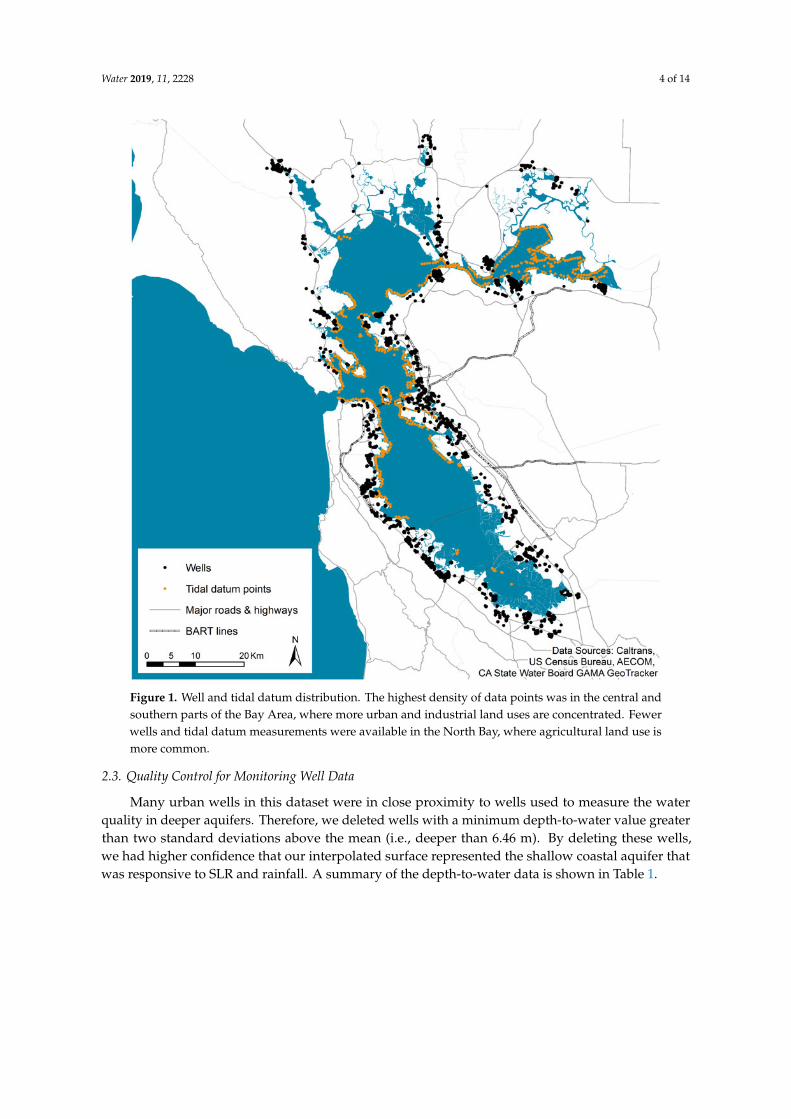
Our methods follow similar studies for Honolulu, HI [5] and three locations in coastal California(excluding the San Francisco Bay Area) [4] but cover a much larger geographic area than either ofthese studies. We used a dataset of groundwater monitoring well measurements that contained valuesfor depth to the water table and covered portions of all nine Bay Area counties [25]. The data pointswere concentrated in heavily developed areas, with fewer wells in the northern Bay Area (Figure 1).We included wells within 1.6 km of the Bay edge to ensure continuity in our interpolated results,although the only results shown were within 1 km of the Bay. We used the San Francisco EstuaryInstitute’s Bay Area Aquatic Resource Inventory delineation of open water and tidal wetland to definethe Bay’s edge [26].

We selected the minimum depth-to-water value for each well during the years 1996–2016. Thisrepresented the seasonal high water table during wetter years, allowing us to estimate the highestelevation of the water table. Where this maximum groundwater elevation occurred, remobilizedpollutants and reduced sewer pipe capacity may have been present in an unusually wet year or duringan exceptionally high tide event.

Water 2019, 11, 2228 4 of 14Water 2019, 11, x FOR PEER REVIEW 4 of 14

Figure 1. Well and tidal datum distribution. The highest density of data points was in the central and southern parts of the Bay Area, where more urban and industrial land uses are concentrated. Fewer wells and tidal datum measurements were available in the North Bay, where agricultural land use is more common.

We selected the minimum depth-to-water value for each well during the years 1996–2016. This represented the seasonal high water table during wetter years, allowing us to estimate the highest elevation of the water table. Where this maximum groundwater elevation occurred, remobilized pollutants and reduced sewer pipe capacity may have been present in an unusually wet year or during an exceptionally high tide event.

2.3. Quality Control for Monitoring Well Data

Many urban wells in this dataset were in close proximity to wells used to measure the water quality in deeper aquifers. Therefore, we deleted wells with a minimum depth-to-water value greater than two standard deviations above the mean (i.e., deeper than 6.46 m). By deleting these wells, we had higher confidence that our interpolated surface represented the shallow coastal aquifer that was responsive to SLR and rainfall. A summary of the depth-to-water data is shown in Table 1.

Figure 1. Well and tidal datum distribution. The highest density of data points was in the central andsouthern parts of the Bay Area, where more urban and industrial land uses are concentrated. Fewerwells and tidal datum measurements were available in the North Bay, where agricultural land use ismore common.

2.3. Quality Control for Monitoring Well Data

Many urban wells in this dataset were in close proximity to wells used to measure the waterquality in deeper aquifers. Therefore, we deleted wells with a minimum depth-to-water value greaterthan two standard deviations above the mean (i.e., deeper than 6.46 m). By deleting these wells,we had higher confidence that our interpolated surface represented the shallow coastal aquifer thatwas responsive to SLR and rainfall. A summary of the depth-to-water data is shown in Table 1.

Water 2019, 11, 2228 5 of 14

Table 1. Summary statistics for well minimum depth-to-water data included in the analysis.

Statistic Value

Count 10,777Minimum 0 mMaximum 6.46 m

Mean 1.95 mMedian 1.75 m

Standard Deviation 1.21 m

2.4. Tidal Data

We also included tidal data points from a dataset produced for the Federal Emergency ManagementAgency and regional agencies [27]. To smooth the interpolated surface toward the Bay, we included603 mean tide line points, and added 0.3 m to the elevation to reflect the expectation that freshwaterusually lies above the mean tide line [28]. Since the tidal water levels varied substantially along theshoreline as a result of the hydrodynamics in San Francisco Bay, tide gauge locations alone wereinsufficient. The tidal dataset we used was calibrated to National Oceanographic and AtmosphericAdministration tide gauges and provided extensive spatial coverage along the Bay shore.

2.5. Analysis

For each well point in the study area, we extracted a ground elevation from the United StatesGeological Survey (USGS) Coastal and Marine Geology Program 2 m digital elevation model (DEM).We then calculated the maximum water table elevation at each well point by subtracting the minimumdepth-to-water value from this ground elevation, following the method used by Hoover et al. [4].Next, we applied a set of interpolation algorithms to the groundwater elevations and tidal data points.A flowchart describing our analysis methods is shown in Figure 2.

Water 2019, 11, x FOR PEER REVIEW 5 of 14

Table 1. Summary statistics for well minimum depth-to-water data included in the analysis.

Statistic Value Count 10,777

Minimum 0 m Maximum 6.46 m

Mean 1.95 m Median 1.75 m

Standard Deviation 1.21 m

2.4. Tidal Data

We also included tidal data points from a dataset produced for the Federal Emergency Management Agency and regional agencies [27]. To smooth the interpolated surface toward the Bay, we included 603 mean tide line points, and added 0.3 m to the elevation to reflect the expectation that freshwater usually lies above the mean tide line [28]. Since the tidal water levels varied substantially along the shoreline as a result of the hydrodynamics in San Francisco Bay, tide gauge locations alone were insufficient. The tidal dataset we used was calibrated to National Oceanographic and Atmospheric Administration tide gauges and provided extensive spatial coverage along the Bay shore.

2.5. Analysis

For each well point in the study area, we extracted a ground elevation from the United States Geological Survey (USGS) Coastal and Marine Geology Program 2 m digital elevation model (DEM). We then calculated the maximum water table elevation at each well point by subtracting the minimum depth-to-water value from this ground elevation, following the method used by Hoover et al. [4]. Next, we applied a set of interpolation algorithms to the groundwater elevations and tidal data points. A flowchart describing our analysis methods is shown in Figure 2.

Figure 2. Flowchart of methods. Key inputs and outputs are shown in italics. Both deterministic and geostatistical methods have been used to predict a water table elevation surface from well data in other studies [29–32]. The dataset used here was not well-suited to kriging because it did not fulfill the assumption of stationarity necessary for this method. Data variance was not constant across the study area and could not be explained by directional trends. Given these limitations for geostatistical methods, we only compared deterministic interpolation methods.

Figure 2. Flowchart of methods. Key inputs and outputs are shown in italics. Both deterministic andgeostatistical methods have been used to predict a water table elevation surface from well data inother studies [29–32]. The dataset used here was not well-suited to kriging because it did not fulfillthe assumption of stationarity necessary for this method. Data variance was not constant across thestudy area and could not be explained by directional trends. Given these limitations for geostatisticalmethods, we only compared deterministic interpolation methods.

To maximize the model accuracy, we compared a variety of methods to determine which wasmost successful at minimizing the prediction error. We compared the root-mean-square error (RMSE)of predicted values from each model using the cross validation function of the ArcGIS Geostatistical

Water 2019, 11, 2228 6 of 14

Analyst toolbox (Table 2). Values of RMSE closer to zero indicated a more accurate model, and valuesof mean error (ME) closer to zero indicated a less biased model. For each interpolation technique,we chose the input parameters (e.g., power, number of neighbors included) that were most successfulat minimizing RMSE, rather than those that produced the smoothest output.

Table 2. Comparison of various tested deterministic interpolation methods.

Maximum Groundwater Elevation

RMSE ME

Inverse Distance Weighting (IDW) 1.237 −0.021

Global Polynomial Interpolation (GPI) 5.114 −0.001

Radial Basis Functions (RBF): Multiquadric 1.167 −0.010

RBF: Completely Regularized Spline 1.579 −0.006

RBF: Spline with Tension 1.482 −0.006

RBF: Inverse Multiquadric 2.638 −0.003

The method that minimized the RMSE most successfully was the multiquadric radial basis function.A scatterplot of the actual water table elevations (elevation from DEM minus minimum measureddepth-to-water) compared to the predicted water table elevations (output from the multiquadric radialbasis function interpolation) is shown in Figure 3. Next, we subtracted the interpolated water tablesurface from the ground surface DEM to produce a depth-to-water map. We excluded areas greaterthan 1 km from the nearest well due to the increased uncertainty introduced by the lack of well or tidaldata points in these areas.

Water 2019, 11, x FOR PEER REVIEW 6 of 14

To maximize the model accuracy, we compared a variety of methods to determine which was most successful at minimizing the prediction error. We compared the root-mean-square error (RMSE) of predicted values from each model using the cross validation function of the ArcGIS Geostatistical Analyst toolbox (Table 2). Values of RMSE closer to zero indicated a more accurate model, and values of mean error (ME) closer to zero indicated a less biased model. For each interpolation technique, we chose the input parameters (e.g., power, number of neighbors included) that were most successful at minimizing RMSE, rather than those that produced the smoothest output.

Table 2. Comparison of various tested deterministic interpolation methods.

Maximum Groundwater Elevation RMSE ME

Inverse Distance Weighting (IDW)

1.237 −0.021

Global Polynomial Interpolation (GPI)

5.114 −0.001

Radial Basis Functions (RBF): Multiquadric 1.167 −0.010

RBF: Completely Regularized Spline

1.579 −0.006

RBF: Spline with Tension 1.482 −0.006

RBF: Inverse Multiquadric

2.638 −0.003

The method that minimized the RMSE most successfully was the multiquadric radial basis function. A scatterplot of the actual water table elevations (elevation from DEM minus minimum measured depth-to-water) compared to the predicted water table elevations (output from the multiquadric radial basis function interpolation) is shown in Figure 3. Next, we subtracted the interpolated water table surface from the ground surface DEM to produce a depth-to-water map. We excluded areas greater than 1 km from the nearest well due to the increased uncertainty introduced by the lack of well or tidal data points in these areas.

Figure 3. Actual water table elevation compared to predicted elevation from the interpolation.The “actual” water table elevation was ground elevation minus the minimum measured depth-to-water.The predicted water table elevation was the value extracted from the raster output of the radial basisfunction interpolation at the well point location. The plot includes points within the final study areaonly (i.e., within 1 km of the Bay edge).

Water 2019, 11, 2228 7 of 14

3. Results

Figure 4 shows the results of our depth-to-water modeling for the coastal Bay Area. A geospatialdata file can be downloaded at https://datadryad.org/stash/dataset/doi:10.6078/D1W01Q We found thata shallow groundwater condition exists in many developed areas in the North Bay including Fairfield,Novato, San Rafael, and Petaluma, although fewer well data points were available for the North Bay ingeneral. Many cities in the East Bay also had shallow groundwater along the Bay-front, placing majorinfrastructure (such as Interstate highways 580 and 880) at risk. Exposure to potential groundwaterflooding was perhaps most severe in the Silicon Valley area, where the minimum depth-to-water wasalready less than one meter in large areas of Mountain View, Redwood City, and San Mateo. Figure 5shows subset maps of groundwater conditions in selected highly urbanized areas.

Water 2019, 11, x FOR PEER REVIEW 7 of 14

Figure 3. Actual water table elevation compared to predicted elevation from the interpolation. The “actual” water table elevation was ground elevation minus the minimum measured depth-to-water. The predicted water table elevation was the value extracted from the raster output of the radial basis function interpolation at the well point location. The plot includes points within the final study area only (i.e., within 1 km of the Bay edge).

3. Results

Figure 4 shows the results of our depth-to-water modeling for the coastal Bay Area. A geospatial data file can be downloaded at https://datadryad.org/stash/dataset/doi:10.6078/D1W01Q We found that a shallow groundwater condition exists in many developed areas in the North Bay including Fairfield, Novato, San Rafael, and Petaluma, although fewer well data points were available for the North Bay in general. Many cities in the East Bay also had shallow groundwater along the Bay-front, placing major infrastructure (such as Interstate highways 580 and 880) at risk. Exposure to potential groundwater flooding was perhaps most severe in the Silicon Valley area, where the minimum depth-to-water was already less than one meter in large areas of Mountain View, Redwood City, and San Mateo. Figure 5 shows subset maps of groundwater conditions in selected highly urbanized areas.

Figure 4. Minimum depth-to-water for the coastal San Francisco Bay Area. Shallow groundwater within one kilometer of the coast is shown in color, with the shallowest areas in red. Our method produced some negative values that suggested groundwater was already emergent, usually where there were no well points in the dataset at the base of a slope or in a valley. These areas (in black) most

Figure 4. Minimum depth-to-water for the coastal San Francisco Bay Area. Shallow groundwaterwithin one kilometer of the coast is shown in color, with the shallowest areas in red. Our methodproduced some negative values that suggested groundwater was already emergent, usually wherethere were no well points in the dataset at the base of a slope or in a valley. These areas (in black) mostlikely had very shallow groundwater with seasonal surface discharges, but a process-based modelwould be needed to quantify the volume.

Water 2019, 11, 2228 8 of 14

Water 2019, 11, x FOR PEER REVIEW 8 of 14

likely had very shallow groundwater with seasonal surface discharges, but a process-based model would be needed to quantify the volume.

Figure 5. Maps of minimum depth-to-water in selected areas. (a) Shallow groundwater conditions were widespread in the Oakland area, including in some low-lying neighborhoods not directly connected to San Francisco Bay. (b) Alviso already experiences groundwater flooding during storms and this flooding will worsen as the sea level rises. The depth-to-water model was likely conservative in this area due to pumping, which results in artificially high depth-to-water values around a landfill. (c) Much of the Silicon Valley coastline had very shallow groundwater, threatening significant properties such as Google’s headquarters. The areas along the shoreline with depth-to-water over 3 m are actively-pumped landfills. (d) Even in Marin County, where the coastline is dominated by steep

Figure 5. Maps of minimum depth-to-water in selected areas. (a) Shallow groundwater conditions werewidespread in the Oakland area, including in some low-lying neighborhoods not directly connectedto San Francisco Bay. (b) Alviso already experiences groundwater flooding during storms and thisflooding will worsen as the sea level rises. The depth-to-water model was likely conservative in thisarea due to pumping, which results in artificially high depth-to-water values around a landfill. (c) Muchof the Silicon Valley coastline had very shallow groundwater, threatening significant properties such asGoogle’s headquarters. The areas along the shoreline with depth-to-water over 3 m are actively-pumpedlandfills. (d) Even in Marin County, where the coastline is dominated by steep bluffs, some low-lyingcoastal flatlands built on fill material were at risk of emergence due to a high groundwater table.

Water 2019, 11, 2228 9 of 14

Projecting Future Conditions

To determine the relationship between 1 m of SLR and a rising water table, we used a simple linearapproximation within 1 km of the Bay edge. This replicated the distance used by Rotzoll and Fletcher [5]in Honolulu, HI based on measured tidal efficiencies, and by Hoover et al. [4] in three smaller areasalong the California coast. Hoover et al. [4] described this linear approximation of the effect of risingsea levels on groundwater depth as conservative, because additional tidal effects would only increasethe impacts on groundwater emergence and shoaling at high tides. Using this linear approximation ofsea level rise impacts, areas of the map in Figure 4 where minimum depth-to-groundwater was lessthan one meter would likely experience groundwater emergence during the wet season of wet yearswith one meter of SLR. The State of California recommended that public agencies consider one meterof SLR likely at the Golden Gate by 2100 under the RCP 8.5 IPCC emissions scenario, and by 2150under the RCP 4.5 and RCP 2.6 scenarios [33].

Figure 6 shows the minimum depth-to-groundwater in the highly urbanized Bay Area with 1 m ofSLR. Our analysis revealed widespread areas where surface flooding from groundwater emergence ispossible. Table 3 reports the extent of flooding from emergent groundwater with 1 m of SLR, comparedto the extent of direct flooding from the Bay with the same SLR, based on projections from the OurCoast, Our Future Flood Map (USGS CoSMoS flood model) [20]. To match the groundwater study area,we excluded areas more than 1 km away from a groundwater monitoring well from the direct SLRflooded area calculation.

Water 2019, 11, x FOR PEER REVIEW 10 of 14

Projecting Future Conditions

To determine the relationship between 1 m of SLR and a rising water table, we used a simple linear approximation within 1 km of the Bay edge. This replicated the distance used by Rotzoll and Fletcher [5] in Honolulu, HI based on measured tidal efficiencies, and by Hoover et al. [4] in three smaller areas along the California coast. Hoover et al. [4] described this linear approximation of the effect of rising sea levels on groundwater depth as conservative, because additional tidal effects would only increase the impacts on groundwater emergence and shoaling at high tides. Using this linear approximation of sea level rise impacts, areas of the map in Figure 4 where minimum depth-to-groundwater was less than one meter would likely experience groundwater emergence during the wet season of wet years with one meter of SLR. The State of California recommended that public agencies consider one meter of SLR likely at the Golden Gate by 2100 under the RCP 8.5 IPCC emissions scenario, and by 2150 under the RCP 4.5 and RCP 2.6 scenarios [33].

Figure 6 shows the minimum depth-to-groundwater in the highly urbanized Bay Area with 1 m of SLR. Our analysis revealed widespread areas where surface flooding from groundwater emergence is possible. Table 3 reports the extent of flooding from emergent groundwater with 1 m of SLR, compared to the extent of direct flooding from the Bay with the same SLR, based on projections from the Our Coast, Our Future Flood Map (USGS CoSMoS flood model) [20]. To match the groundwater study area, we excluded areas more than 1 km away from a groundwater monitoring well from the direct SLR flooded area calculation.

Figure 6. Future groundwater flooding. This map shows areas where groundwater is likely to emerge as surface flooding with 1 m of sea level rise (SLR). However, ponding may not necessarily occur in all of these areas, as the model does not account for surface discharge.

Figure 6. Future groundwater flooding. This map shows areas where groundwater is likely to emergeas surface flooding with 1 m of sea level rise (SLR). However, ponding may not necessarily occur in allof these areas, as the model does not account for surface discharge.

Water 2019, 11, 2228 10 of 14

Table 3. Comparison of flood extent from direct tidal flooding due to SLR and groundwater emergencedue to SLR intrusion.

Extent of Potential Flooding with 1 m SLR, km2 (% of Total)

County Direct SLRonly 1

EmergentGroundwater only

Both Direct SLR 1 andEmergent Groundwater

Total

Alameda 3.3 (8%) 28.3 (72%) 7.7 (20%) 39.3Contra Costa 0.7 (3%) 19.5 (87%) 2.2 (10%) 22.5

Marin - 9.1 (65%) 4.8 (35%) 13.9Napa - 8.2 (98%) 0.2 (2%) 8.4

San Francisco - 4.3 (88%) 0.6 (12%) 4.8San Mateo 11.7 (30%) 8.3 (21%) 19.0 (49%) 39.1Santa Clara 7.3 (56%) 2.3 (18%) 3.5 (27%) 13.1

Solano 1.3 (6%) 15.6 (68%) 6.1 (26%) 23.0Sonoma 1.2 (9%) 9.3 (73%) 2.2 (17%) 12.7

Total 25.6 (14%) 104.9 (59%) 46.2 (26%) 176.81 From the Our Coast, Our Future Flood Map [20], with 1 m of SLR and no storm event. The area calculation fordirect SLR matches the extent of the groundwater study area; (1) areas greater than 1 km from well points wereexcluded, and (2) we assumed that the existing water line was the extent of open water and tidal wetland from theSan Francisco Estuary Institute’s Bay Area Aquatic Resource Inventory [26].

The results of our analysis, based on an interpolation of empirical groundwater well data and alinear relationship between SLR and groundwater levels, can be used to identify hotspots that requirea second phase of analysis using higher-resolution elevation and hydrologic data, field measurementsof tidal efficiency, and process-based models. Process-based models developed at smaller geographicscales may be able to account for recharge and discharge, the diminishing influence of SLR inland fromthe coast, wave run-up, and variations in geologic and infrastructure conditions.

4. Discussion

We created an interpolated surface that estimated the depth of shallow groundwater for 489 squarekilometers of San Francisco Bay’s coastline using measured depth-to-water and tidal data. This rapidassessment method indicated that many parts of the Bay Area coastline are vulnerable to risinggroundwater. Based on these results, many San Francisco Bay Area communities should conductfurther modeling studies to prepare for potential flooding from groundwater, in addition to directflooding from SLR. Our study suggested that there is significant potential for groundwater flooding inimportant Silicon Valley economic hubs (e.g., Mountain View, East Palo Alto, Redwood City), East Baycities with fast-growing populations (e.g., Oakland, Hayward, Fremont), and major transportationinfrastructure, including freeways (e.g., Interstate 580) and airports (Oakland International Airport,San Francisco International Airport). Our results indicate that flooding from emergent groundwatercould impact more land by area than direct SLR flooding, with a SLR scenario of one meter in sevenof the nine Bay Area counties, and in the region as a whole (Table 3). However, the calculated areaimpacted by emergent groundwater does not account for surface discharge to streams and otherwater bodies.

In addition to groundwater emergence, risks posed to developed areas include increased infiltrationand inflow of underground water and wastewater pipes [15], and increased liquefaction risks inactive seismic zones. Rising groundwater can also mobilize contaminants from wastewater and legacysoil pollution, producing human and ecosystem health risks. Groundwater emergence is likely tooccur even where levees and seawalls are built to serve as barriers to saltwater coastal inundation.These structures alone will be inadequate to prevent flooding and other hazards without additionaladaptation measures.

Water 2019, 11, 2228 11 of 14

5. Conclusions

We used a rapid assessment interpolation method to create the first depth-to-groundwater mapfor the San Francisco Bay shore zone. The empirical data we used reflects existing human impactsfrom pumping, storm sewer infiltration, and leaky water pipes in a complex urban environment.We maximized the accuracy of the interpolated surface map by testing a variety of methods and selectingthe one that minimized errors. The results of the analysis revealed widespread shallow groundwaterconditions along most of the shore of San Francisco Bay. Using the conservative assumption of alinear relationship between SLR and shallow, unconfined groundwater depth within one kilometer ofthe shore, we showed that many densely developed areas are at risk from rising and even emergentgroundwater as the sea level rises.

The method presented here is useful as a rapid assessment technique for comparing relativeexposure to groundwater hazards and identifying hotspots where localized dynamic modeling isneeded [15,34,35]. The minimum depth-to-water surface shown here did not represent a particularpoint in time, but rather an estimate based on the shallowest measurement taken at each monitoringwell in the dataset during the study timeframe. Sampling was not consistent over time in thisbest-available dataset. Therefore, seasonal changes in precipitation and infiltration were not capturedby this minimum depth-to-water method, although they are an important consideration [30]. Since itwas empirical rather than modeled, the dataset we used for this interpolation reflected human impactson coastal groundwater, including current pumping and leaky pipes. In many areas, the results shownhere were influenced by local leachate pumping at landfills or other groundwater pumping that wasalready in place to prevent flooding.

Any interpolation-based method contains errors. More consistent sample point coveragewould have reduced the level of error introduced by interpolation. Additionally, the simple linearapproximation we used to estimate rising groundwater levels due to SLR did not account for a numberof factors that would have been important to consider in a more nuanced modeling effort. Additionalfactors to consider in future refinements of this technique include the diminishing influence of SLRinland from the coast, the potential effects of tides, waves, and extreme rainfall events, and the needfor more accurate local measurements to establish the effects of different geologic conditions andunderground pipe and pump systems on the level of groundwater rise. Modeling efforts incorporatingmeasurements of tidal influence and groundwater flow, such as those that Habel et al. conductedin regard to Honolulu, HI [36], are needed in the areas that were identified as potential hotspots byour method.

While previous studies established the existence of rising groundwater due to SLR [2,4–6,9,10,22,31],as well as the potential impact at case study sites [2,4,5,28,31,37], this paper provides a method for building aregional-scale view of the potentially widespread impacts on surface flooding, underground infrastructure,and the health of people and ecosystems. Understanding the full range of SLR impacts is essential forprioritizing adaptation investments, and selecting appropriate strategies in coastal cities [15,35,36]. Otherlow-lying urban areas around the world with shallow and unconfined coastal aquifers have an urgentneed to identify the potential for future groundwater flooding as a result of sea level rise. In easternand southeastern US, major metropolitan regions around rivers and bays such as Boston, New York,Philadelphia, Baltimore, Washington DC, Norfolk, Charleston, Ft. Lauderdale, Miami, Tampa, andGalveston could benefit from similar assessment methods for groundwater flooding that make use ofexisting groundwater quality datasets. On the west coast, Seattle, Tacoma, and many smaller citiesand towns on bays along the Oregon, Washington, and California coasts are likely to face groundwaterflooding. Many low-lying cities along bays and deltas in northwestern Europe, coastal areas of the UnitedKingdom, coastal Africa, South America, and Southeast Asia face similar threats. The rapid assessmentmethod presented here provides a valuable approach for the identification of hotspots where risinggroundwater poses a threat to urban development and human health. Once hotspots are identified,process-based groundwater data collection and modeling efforts will be needed at a local scale to more

Water 2019, 11, 2228 12 of 14

fully represent the dynamics of rising groundwater in coastal zones and to account for variables such asprojected future changes in subsidence, recharge, and discharge rates.

Author Contributions: Conceptualization, K.H.; methodology, K.H. and C.M.; formal analysis, E.P.; data curation,E.P.; writing—original draft preparation, E.P.; writing—review and editing, K.H. and C.M.; visualization, E.P.;supervision, K.H.; funding acquisition, K.H.

Funding: This research was partially supported by a contract with Alameda County.

Acknowledgments: We would like to thank the CA State Water Board for supporting our analysis of their welldata. Open access publication was made possible in part by support from the Berkeley Research Impact Initiative(BRII), sponsored by the UC Berkeley Library.

Conflicts of Interest: The authors declare no conflict of interest.

References

1. Intergovernmental Panel on Climate Change. Climate Change 2013: The Physical Science Basis. Contribution ofWorking Group I to the Fifth Assessment Report of the Intergovernmental Panel on Climate Change; CambridgeUniversity Press: Cambridge, UK; New York, NY, USA, 2013.

2. Bjerklie, D.M.; Mullaney, J.R.; Stone, J.R.; Skinner, B.J.; Ramlow, M.A. Preliminary Investigation of the Effects ofSea-Level Rise on Groundwater Levels in New Haven, Connecticut; U.S. Geological Survey: Reston, VA, USA,2012; p. 46.

3. Cooper, H.H. Sea Water in Coastal Aquifers; US Government Printing Office: Washington, DC, USA, 1964.4. Hoover, D.J.; Odigie, K.O.; Swarzenski, P.W.; Barnard, P. Sea-level rise and coastal groundwater inundation

and shoaling at select sites in California, USA. J. Hydrol. Reg. Stud. 2017, 11, 234–249. [CrossRef]5. Rotzoll, K.; Fletcher, C.H. Assessment of groundwater inundation as a consequence of sea-level rise. Nat. Clim.

Chang. 2012, 3, 477–481. [CrossRef]6. Chesnaux, R. Closed-form analytical solutions for assessing the consequences of sea-level rise on groundwater

resources in sloping coastal aquifers. Hydrogeol. J. 2015, 23, 1399–1413. [CrossRef]7. Werner, A.D.; Simmons, C.T. Impact of Sea-Level Rise on Sea Water Intrusion in Coastal Aquifers. Ground

Water 2009, 47, 197–204. [CrossRef] [PubMed]8. Chang, S.W.; Clement, T.P.; Simpson, M.J.; Lee, K.-K. Does sea-level rise have an impact on saltwater

intrusion? Adv. Water Resour. 2011, 34, 1283–1291. [CrossRef]9. Michael, H.A.; Russoniello, C.J.; Byron, L.A. Global assessment of vulnerability to sea-level rise in

topography-limited and recharge-limited coastal groundwater systems. Water Resour. Res. 2013, 49, 2228–2240.[CrossRef]

10. Nuttle, W.K.; Portnoy, J.W. Effect of rising sea level on runoff and groundwater discharge to coastal ecosystems.Estuar. Coast. Shelf Sci. 1992, 34, 203–212. [CrossRef]

11. Galloway, D.L.; Burbey, T.J. Review: Regional land subsidence accompanying groundwater extraction.Hydrogeol. J. 2011, 19, 1459–1486. [CrossRef]

12. Scott, J.M.; Schipper, J. Gap analysis: A spatial tool for conservation planning. In Principles of ConservationBiology, 3rd ed.; Groom, M.J., Meffe, G.K., Carroll, C.R., Eds.; Sinauer: Sunderland, MA, USA, 2006;pp. 518–519.

13. Jamei, Y.; Rajagopalan, P.; Sun, Q. (Chayn) Spatial structure of surface urban heat island and its relationshipwith vegetation and built-up areas in Melbourne, Australia. Sci. Total Environ. 2019, 659, 1335–1351.[CrossRef]

14. Rembold, F.; Meroni, M.; Urbano, F.; Csak, G.; Kerdiles, H.; Perez-Hoyos, A.; Lemoine, G.; Leo, O.; Negre, T.ASAP: A new global early warning system to detect anomaly hot spots of agricultural production for foodsecurity analysis. Agric. Syst. 2019, 168, 247–257. [CrossRef]

15. Hummel, M.A.; Berry, M.S.; Stacey, M.T. Sea Level Rise Impacts on Wastewater Treatment Systems Along theU.S. Coasts. Earth’s Future 2018, 6, 622–633. [CrossRef]

16. Smith, R.A. Center for Operational Oceanographic Products and Services. In Historical Golden Gate TidalSeries; NOAA: Silver Spring, MD, USA, 2002.

17. Knowles, N. Potential Inundation Due to Rising Sea Levels in the San Francisco Bay Region. San Franc.Estuary Watershed Sci. 2010, 8. [CrossRef]

Water 2019, 11, 2228 13 of 14

18. Vandever, J.; Lightner, M.; Kassem, S.; Guyenet, J.; Mak, M.; Bonham-Carter, C. Adapting to Rising Tides:Bay Area Sea Level Rise Analysis and Mapping Project; San Francisco Bay Conservation and DevelopmentCommission, Metropolitan Transportation Commission, Bay Area Toll Authority, AECOM, San Francisco,CA: 2017. Available online: http://www.adaptingtorisingtides.org/wp-content/uploads/2018/07/BATA-ART-SLR-Analysis-and-Mapping-Report-Final-20170908.pdf (accessed on 22 April 2018).

19. Takekawa, J.Y.; Thorne, K.M.; Buffington, K.J.; Spragens, K.A.; Swanson, K.M.; Drexler, J.Z.;Schoellhamer, D.H.; Overton, C.T.; Casazza, M.L. Final Report for Sea-Level Rise Response Modeling forSan Francisco Bay Estuary Tidal Marshes; Open-File Report; U.S. Geological Survey: Reston, VA, USA, 2013;p. 171.

20. USGS. Point Blue Conservation Science OCOF Our Coast, Our Future Flood Map. Available online:http://data.pointblue.org/apps/ocof/cms/index.php?page=flood-map (accessed on 19 June 2019).

21. Shirzaei, M.; Bürgmann, R. Global climate change and local land subsidence exacerbate inundation risk tothe San Francisco Bay Area. Sci. Adv. 2018, 4, eaap9234. [CrossRef] [PubMed]

22. Masterson, J.P.; Garabedian, S.P. Effects of Sea-Level Rise on Ground Water Flow in a Coastal Aquifer System.Ground Water 2007, 45, 209–217. [CrossRef]

23. Planert, M.; Williams, J.S. Groundwater Atlas of the United States: California, Nevada (HA 730-B, Coastal BasinsAquifers); USGS: 1995. Available online: https://pubs.usgs.gov/ha/ha730/ch_b/B-text4.html (accessed on14 July 2017).

24. Ferriz, H. Groundwater resources of northern California: An overview. Eng. Geol. Pract. North. Calif. Bull.2001, 210, 19–47.

25. CA State Water Resources Control Board GeoTracker. Available online: http://geotracker.waterboards.ca.gov/data_download_by_county (accessed on 29 January 2017).

26. San Francisco Estuary Institute Bay Area Aquatic Resource Inventory (BAARI) Version 2.1 GIS Data. Availableonline: http://www.sfei.org/data/baari-version-21-gis-data (accessed on 14 October 2016).

27. Mak, M.; Harris, E.; Lightner, M.; Vandever, J.; May, K. San Francisco Bay Tidal Datums and Extreme TidesStudy; Prepared for the Federal Emergency Management Agency by AECOM: Oakland, CA, USA, 2016;Available online: https://www.adaptingtorisingtides.org/wp-content/uploads/2016/05/20160429.SFBay_Tidal-Datums_and_Extreme_Tides_Study.FINAL_.pdf (accessed on 25 October 2016).

28. Moss, A. Coastal Water Table Mapping: Incorporating Groundwater Data into Flood Inundation Forecasts.Master’s Thesis, Duke University, Durham, NC, USA, 2016.

29. Akkala, A.; Devabhaktuni, V.; Kumar, A. Interpolation techniques and associated software for environmentaldata. Environ. Prog. Sustain. Energy 2010, 29, 134–141. [CrossRef]

30. Buchanan, S.; Triantafilis, J. Mapping Water Table Depth Using Geophysical and Environmental Variables.Ground Water 2009, 47, 80–96. [CrossRef]

31. Cooper, H.M.; Zhang, C.; Selch, D. Incorporating uncertainty of groundwater modeling in sea-level riseassessment: A case study in South Florida. Clim. Chang. 2015, 129, 281–294. [CrossRef]

32. Sun, Y.; Kang, S.; Li, F.; Zhang, L. Comparison of interpolation methods for depth to groundwater andits temporal and spatial variations in the Minqin oasis of northwest China. Environ. Model. Softw.2009, 24, 1163–1170. [CrossRef]

33. Griggs, G.; Arvai, J.; Cayan, D.; DeConto, R.; Fox, J.; Fricker, H.; Kopp, R.; Tebaldi, C.; Whiteman, E.; CaliforniaOcean Protection Council Science Advisory Team Working Group. Rising Seas in California: An Update onSea-Level Rise Science; California Ocean Science Trust: 2017. Available online: http://www.oceansciencetrust.org/

wp-content/uploads/2017/04/OST-Sea-Level-Rising-Report-Final_Amended.pdf (accessed on 9 May 2017).34. All Bay Collective, Resilient by Design Bay Area Challenge. The Estuary Commons: People, Place, and

a Path Forward 2018. Available online: http://www.resilientbayarea.org/estuary-commons (accessed on20 August 2019).

35. SFEI and SPUR. San Francisco Bay Shoreline Adaptation Atlas: Working with Nature to Plan for Sea Level RiseUsing Operational Landscape Units; San Francisco Estuary Institute: Richmond, CA, USA, 2019.

Water 2019, 11, 2228 14 of 14

36. Habel, S.; Fletcher, C.H.; Rotzoll, K.; El-Kadi, A.I. Development of a model to simulate groundwaterinundation induced by sea-level rise and high tides in Honolulu, Hawaii. Water Res. 2017, 114, 122–134.[CrossRef]

37. Luoma, S.; Okkonen, J. Impacts of Future Climate Change and Baltic Sea Level Rise on GroundwaterRecharge, Groundwater Levels, and Surface Leakage in the Hanko Aquifer in Southern Finland. Water2014, 6, 3671–3700. [CrossRef]

© 2019 by the authors. Licensee MDPI, Basel, Switzerland. This article is an open accessarticle distributed under the terms and conditions of the Creative Commons Attribution(CC BY) license (http://creativecommons.org/licenses/by/4.0/).