Combustor Dilution Hole Placement and Its Effecton the Turbine Inlet Flowfield

Michael Leonetti,∗ Stephen Lynch,† and Jacqueline O’Connor‡

Pennsylvania State University, University Park, Pennsylvania 16802

and

Sean Bradshaw§

United Technologies—Pratt & Whitney, East Hartford, Connecticut 06108

DOI: 10.2514/1.B36308

Dilution jets in a gas turbine combustor are used to oxidize remaining fuel from the main flame zone in the

combustor and to homogenize the temperature field upstream of the turbine section through highly turbulentmixing.

The high-momentum injection generates high levels of turbulence and very effective turbulent mixing. However,

mean flow distortions and large-scale turbulence can persist into the turbine section. In this study, a dilution hole

configuration was scaled from a rich-burn–quench–lean-burn combustor and used in conjunction with a linear vane

cascade in a large-scale, low-speed wind tunnel. Mean and turbulent flowfield data were obtained at the vane leading

edge with the use of high-speed particle image velocimetry to help quantify the effect of the dilution jets in the turbine

section. The dilution hole pattern was shifted (clocked) for two positions such that a large dilution jet was located

directly upstream of a vane or in between vanes. Time-averaged results show that the large dilution jets have a

significant impact on the magnitude and orientation of the flow entering the turbine. Turbulence levels of 40% or

greater were observed approaching the vane leading edge, with integral length scales of approximately 40% of the

dilution jet diameter. Incidence angle and turbulence level were dependent on the position of the dilution jets relative

to the vane.

Nomenclature

Cax = vane axial chordCp = �Ps − Ps;in�∕0.5ρU2, nondimensional static

pressureD = dilution jet diameterI = �ρU2�jet∕�ρU2�∞, momentum flux ratioLx−s = ∫ ∞

0 Rii�x; z;Δx� dΔx, spatial axial integrallength scale

Lx−t = u�x; z� � ∫ ∞0 Rii�x; z;Δt� dΔt, temporal axial

integral length scale_m = ρUA, mass flow rateP = pressurep = vane pitchRii�x; z;Δt� = hu 0�x; z; t� � u 0�x; z; t� Δt�i∕u2rms�x; z�, tem-

poral autocorrelation coefficientRii�x; z;Δx� = hu 0�x; z; t� � u 0�x � Δx; z; t�i∕urms�x; z� �

urms�x � Δx; z�, spatial autocorrelationcoefficient

S = test-section spans = surface distance along vaneTuloc = �urms∕Uloc� � 100, axial component of turbu-

lence intensity normalized by the local velocitymagnitude, %

Tum = �urms∕Um−avg� � 100, axial component ofturbulence levels normalized by the turbineinlet mass-average velocity magnitude, %

Twm = �wrms∕Um−avg� � 100, pitchwise component ofturbulence levels normalized by the turbine inletmass-average velocity magnitude, %

U = velocity magnitude

Ujet−plenum =�����������������������������������������������2 � �P∞ − Pplenum�∕ρ∞

p, dilution jet velocity

using plenum and mainstream pressure data

Ujet−pitot =������������������������2 � ΔP∕ρjet

p, dilution jet velocity determined

using pitot probe dataUm = U∕Um−avg, velocity magnitude normalized by

the turbine inlet mass average velocityUm−avg = _mcombustor �

P_mdilution jets∕ρ∞ � S �W, mass-

averaged turbine inlet velocity magnitudeu = axial component of velocityv = spanwise component of velocityW = combustor widthw = pitchwise component of velocityx = axial directiony = spanwise directionz = pitchwise directionα = incidence angleυ = kinematic viscosityρ = densityh i = time average of a quantity

Subscripts

jet = jet propertyloc = normalized by a local velocity magnitudem = normalized by a turbine inlet mass-average

velocity magnitudem-avg = mass-averaged valuerms = root mean square∞ = mainstream property

I. Introduction

T HE combustor section of a gas turbine engine burns fuel and airto create the high-enthalpy fluid needed to turn the turbines. In a

rich-burn–quench–lean-burn (RQL) style of combustor, popular inaviation gas turbines, large dilution jets are injected into thecombustor downstream of the initial rich combustion zone to oxidize

Received 29 April 2016; revision received 17 August 2016; accepted forpublication 15 September 2016; published online 11 January 2017. Copyright© 2016 byMichael Leonetti, Stephen Lynch, Jacqueline O’Connor, and SeanBradshaw. Published by the American Institute of Aeronautics andAstronautics, Inc., with permission. All requests for copying and permissionto reprint should be submitted to CCC at www.copyright.com; employ theISSN 0748-4658 (print) or 1533-3876 (online) to initiate your request. Seealso AIAA Rights and Permissions www.aiaa.org/randp.

*Graduate Assistant, Department of Mechanical and Nuclear Engineering,114 Research West.

†Assistant Professor, Department of Mechanical and Nuclear Engineering,331 Reber. Senior Member AIAA.

‡Assistant Professor, Department of Mechanical and Nuclear Engineering,111 Research East. Senior Member AIAA.

§Technical Team Lead, Combustor Aero/Thermal, 400 Main St.

750

JOURNAL OF PROPULSION AND POWER

Vol. 33, No. 3, May–June 2017

Dow

nloa

ded

by P

EN

NSY

LV

AN

IA S

TA

TE

UN

IVE

RSI

TY

on

Apr

il 13

, 201

8 | h

ttp://

arc.

aiaa

.org

| D

OI:

10.

2514

/1.B

3630

8

remaining fuel from the main combustion zone. The jets also help tohomogenize the flow temperature through turbulent mixing. Thiscreates high turbulence levels and potentially a nonuniform flowfield(if mixing is insufficient) that enters the turbine section. Thisoncoming flowfield can be very detrimental to the turbine vanedurability because the gas temperatures can exceed the vane meltingtemperature. A current trend in commercial aviation gas turbines isincreasingly smaller engine cores to achieve ultrahigh bypass ratiosfor high propulsive efficiency. Thus, combustors continue to shortenin length, potentially positioning dilution jets closer to thedownstream vanes. Although the turbine vanes are designed withadvanced cooling techniques to survive the hot gas temperatures, thecooling strategy effectiveness is highly dependent on accurateknowledge of the turbine inflow conditions.The goal of this work is to provide some understanding of the

dilution jet’s impact on the flowfield approaching the turbine vanethrough high-speed, spatially resolved flowfield measurements. Thisunderstanding can be used to aid in the improvement of vane coolingefficiency. It has also shown the importance of integrated designbetween the combustor and turbine sections. The results could also beapplied to improving computational predictions of turbine flow byproviding temporally and spatially resolved turbulence and flowfieldcharacteristics at the turbine inlet plane.

II. Relevant Literature

Many experimental and numerical studies have investigatedcombustor and turbine flowfields separately, but few have bothspatially and temporally investigated the flowfield as it exits acombustor and enters the turbine section. For this study, we considerthe dilution jets and their effect on turbulence levels and mean flowdistortion. These dilution jets are effectively jets in crossflow, whichhave been investigated heavily in the past.Fric and Roshko [1] showed that a jet injected into a crossflow

creates four types of coherent structures in the near field of the jet: jetshear-layer vortices, horseshoe vortices, wake vortices, and acounter-rotating vortex pair. All of these structures contribute to thetimemean and turbulent flowfield downstream of the jet. However, ina gas turbine combustor, these jets are confined and in closeinteraction with neighboring jets. Several studies have investigatedconfined jet behavior in combustorlike geometries. Holdeman [2]found that jet trajectories in an annulus are similar to those in arectangular duct for the same momentum flux ratio. Holdeman et al.[3] also found that jet penetration was dependent on momentum fluxratio and therefore the flow distribution and mixing. In-line dilutionjet configurations had both better initial mixing and downstreammixing for momentum flux ratios less than 64, relative to staggereddilution jet configurations. Holdeman et al. [4] compared velocityprofiles of dilution jets with the same momentum flux ratio but withvarying density ratios and found that density ratio only had a second-order effect on the profiles. These studies, among others, indicate thatthe momentum flux ratio and jet alignment have the largest effect onjet penetration and mixing.However, many prior studies of dilution mixing have focused on

time-mean results. When jets are injected into crossflow theygenerate a large amount of turbulence, which can impact vane heattransfer and effectiveness of cooling techniques. Most studies havefound that turbulence levels entering the turbine can range between10 and 20%,with integral length scales on the order of the dilution jetdiameter. These results vary with dilution jet arrangement, hole size,hole location, and momentum flux ratio. Cha et al. [5] foundturbulence levels at the combustor–turbine interface of approx-imately 35% and length scales of up to 25% of the vane chord length.Vakil and Thole [6] used a nonreacting cold-flow combustor withboth dilution and film cooling holes that had measured turbulencelevels of 20%. Kidney-shaped thermal fields were created from thecounter-rotating vortices generated by the jets; this created a turbineinlet plane that had anisotropic turbulence and nonuniform thermalfields. Barringer et al. [7] conducted a similar experiment, whichyielded slightly lower turbulence levels in the range of 15–18% for anisothermal combustor. Ames and Moffat [8] also found similar

turbulence levels generated in their simulated isothermal combustor,which reached as high as 19%. This study also determined that theturbulent length scale in their flowfieldwas on the order ofmagnitudeof the dilution hole diameter. These high freestream turbulence levelsare well-known to augment heat transfer and disperse film cooling,particularly at the stagnation point on a vane (Ames [9], Gandavarapuand Ames [10], Ames [11], Nasir et al. [12], Radomsky andThole [13]).Most prior studies investigating the effects of high freestream

turbulence on heat transfer augmentation have used simulatedturbulence from bar grids. Van Fossen et al. [14] studied the effect ofhigh freestream turbulence, generated by bar grids, on stagnation heattransfer. In general, stagnation region heat transfer increased withdecreasing turbulence length scale and increasing freestreamturbulence level. In their work, a correlation was proposed to predictthe effect of augmentation of stagnation heat transfer; however, thiscorrelation was based on isotropic turbulence, which may not beappropriate for the vane in an engine. In fact, their correlationunderpredicted the stagnation heat transfer by up to 11% forturbulence from a parallel-wire grid, which generated significantturbulence anisotropy. Ames [9] considered higher levels ofturbulence and their effects on vane heat transfer using both bar-gridturbulence as well as dilution jets from a simulated combustor. Thisstudy concluded that an energy scaleLu, which incorporates turbulentkinetic energy and length scale, had a significant impact on thestagnation and pressure surface heat transfer. Gandavarapu and Ames[10] found that grid-generated turbulence correlations underpredictedvane heat transfer augmentation, whereas their scaling parameter,based on turbulence level, Reynolds number, and turbulent lengthscale, overpredicted heat transfer augmentation for a very-large-diameter leading edge (i.e., high Reynolds number). In general,correlations can be found to bound vane stagnation heat transferaugmentation at high turbulence levels but may not be appropriate forother situations, likely due to an incomplete understanding of thenature of the turbulence at high turbulence levels.Growth in computational capability and the continued desire to

optimize turbine engines has led to increased interest in simulatingthe combustor and turbine simultaneously so that assumptions aboutboundary conditions between the two are eliminated. Priorcomputational simulations often only focused on either thecombustor or turbine section, generally keeping the two portions ofthe engine separate because modeling both can be computationallyintensive. Experimental results have shown that the flowfield at thecombustor outlet is highly turbulent and spatially nonuniform,although often boundary conditions used at the turbine inlet do notrepresent this. Another potential issue from performing separatesimulations is the absence of the vane’s impact in the combustorsimulation; this is especially true for combustors with dilution jetspositioned near the turbine inlet. Cha et al. [15] showed throughexperimental and computational studies that the nozzle guide vane’s(NGV) potential field has an effect on the upstream combustor flow.Cha et al. found that the NGV’s impact occurs well before thecombustor–turbine interaction plane where many combustor-onlystudies end. Salvadori et al. [16] performed two Reynolds-averagedNavier–Stokes (RANS) simulations, one where the combustor–vaneinteraction were modeled separately with no feedback between thetwo computational domains, and a second simulation with couplingbetween the two domains. They found that the decoupled simulationdid a poor job of predicting the flow entering the vane section. Thisresulted in a turbine simulation that overpredicted the impact of swirl,while also failing to capture the dilution hole clocking effects. Theyrecommended the use of at least a coupled approach for its moreaccurate flowfield entering the turbine inlet. A steady RANSsimulation conducted by Stitzel and Thole [17] showed that the use ofa two-dimensional turbine inlet boundary condition near the endwall, as is typically done in practice, was inaccurate; instead, the exitflowfield from a realistic combustor exhibited three-dimensionalbehaviors with nonuniformities in temperature, pressure, andvelocity.Insinna et al. [18] also used a coupled combustor/turbine

simulation, which found similar nonuniformities at the turbine inlet

LEONETTI ETAL. 751

Dow

nloa

ded

by P

EN

NSY

LV

AN

IA S

TA

TE

UN

IVE

RSI

TY

on

Apr

il 13

, 201

8 | h

ttp://

arc.

aiaa

.org

| D

OI:

10.

2514

/1.B

3630

8

in the radial and tangential directions. Thermal differences on thevane and changes in incidence angle of the oncoming flow were alsofound using this coupled model. Prenter et al. [19] comparedsimulations and experiments from an annular combustor–turbine rig,which included dilution jets and reacting flow. Each steady RANSturbulence model predicted different temperature profiles at theturbine inlet plane and underpredicted jet mixing as well as lateralspreading. Cha et al. [5] noted that higher-fidelity modeling (large-eddy simulation) more accurately predicted the turbulence intensitiesfound at the combustor–turbine interface in their experiment. Simplymodeling the combustor and turbine together may not be enough toensure accurate results; higher-fidelity unsteadymodels are needed toaccurately predict the large turbulent structures stemming from theunsteady combustor flowfield.The purpose of this study is to experimentally characterize the

mean and unsteady flowfield entering the turbine inlet to provide amore complete understanding of the incoming flow conditions.Dilution hole placement is considered in this study by alternating thepitchwise location of the holes with respect to the vanes. A dilutionhole momentum flux ratio representative of RQL combustor designsis used, based on the importance of momentum flux ratio in the jetbehavior as described earlier. Although heat transfer measurementswere not taken during this study, the likely impact of the incomingflowfield on vane heat transfer is mentioned.

III. Experimental Setup

This experiment used a simulated combustor and scaled vanes in alow-speed large-scale wind tunnel shown in Fig. 1. This wind tunnelhas been used in previous investigations of combustor and otherdilution flow studies (Vakil and Thole [6], Barringer et al. [7], Stitzeland Thole [17]). For those studies, the combustor geometry wasbased on older technology and had a significant flow areaconvergence upstream of the vane, which was eliminated for thisstudy. Also, the previous dilution studies were at a larger scale andthus modeled a single combustor sector with two rows of dilution,whereas this study models two sectors with a single row of dilution.Upstream of the test section, the flow is split into the main core

flow section and twobypass flow sections. The flow can be controlledto divert the wanted amount of flow into the bypass sections. Theexperiments presented in this paper were conducted isothermally.The core flow was used as the mainstream combustor flow, whereasthe two bypass flow sections were used as plenums to feed thedilution flow. The tunnel has the capability to insert different testsections of varying span. Vane test sections are inserted at the cornerof the tunnel to complete the recirculating loop. The first vane used inthe experiment was based on a commercial engine design and isdescribed by Gibson et al. [20]. The vane test section has five vanes,an inlet span height of 1.912Cax, a pitch of 1.215Cax, and an inletReynolds number based on axial chord of 64,000. A turbulence bargrid is located upstream of the dilution to provide initial turbulentflow;without dilution, it results in a 7% turbulence level at the turbineinlet. The large-scalewind tunnel does not have the capabilities to run

compressible flow experiments; therefore, Mach number in thecascade was not matched to engine conditions, but the Reynoldsnumber was matched due to the large scale. Previous studies haveshown that Mach number has little effect on secondary flowfields inthe vane passage (Perdichizzi [21], Hermanson and Thole [22]).Mach number was also shown to have little to no effect on pressure-side heat transfer, although suction-side surface pressure and heattransfer are affected by Mach number, as shown by Nealy et al. [23]and Arts and De Rouvroit [24]. Note that this study is focused on theleading-edge region of the first vane, where velocities are low evenfor transonic vanes (Nix et al. [25], Barringer et al. [26]). Finally, theexperiment was conducted without the addition of fuel and reactiveproducts, although studies such as those conducted by Zimmerman[27] and Moss and Oldfield [28] have shown that turbulencelevels values downstream of combustion were unaffected by thecombustion process.For this study, a commercially relevant RQL-style combustor was

geometrically scaled for the large wind tunnel and inserted upstreamof the vane test section. Because of vane geometry constraints, theHoldeman parameter (Holdeman [2]) of the scaled combustorgeometry was smaller than the optimum of 5.0 (Holdeman [2]) forcombustors with offset dilution hole centerlines, which would resultin some underpenetration of the dilution jets relative to an optimumconfiguration. The primary feature scaled from the engine conditionwas the dilution hole geometry; other features of the combustor suchas liner cooling were not included in this work. Note that, in thisstudy, the combustor simulator did not have swirled flowapproaching the dilution holes. The level of swirl normally presentin an aeroengine RQL combustor was presumed to be negligiblerelative to the effect of high-momentum flux dilution injection. Thestudy by Cha et al. [15] for a similar RQL geometry also indicatedlittle effect of upstream swirl on dilution jet trajectory.The momentum flux ratio of the dilution was matched to a

representative engine condition. Momentum flux ratio wasdetermined to be the most significant aerodynamic parameterbecause this will determine the jet’s trajectory, as discussed earlier.Because the low-speed wind tunnel cannot match the density ratiosfound in a real engine, themass addition of each holewas notmatchedto the engine condition; however, the jet penetration is the primaryfactor in the jet mixing behavior. Note also that, in the wind tunnel,the vane cascade geometry is planar (not annular), and so the innerdiameter (ID) and outer diameter (OD) walls in the wind tunnel havethe same arc length. In the wind-tunnel implementation, the bottomwall of the tunnel was designated as theOD endwall, and the topwallwas designated as the ID endwall. This is because the direction of thevanes in the cascade is reversed relative to convention. The vanes andthe coordinate system used in this experiment can be seen in Fig. 2.The dashed line in Fig. 2b shows the measurement plane that wasinvestigated in this study.The simulated combustor consisted of two full combustor sectors,

where each sector had four dilution holes with an alternating patternof large and small diameter holes. The OD and ID sectors had thesame number of holes. This meant that both the OD and ID sectorshad eight dilution holes each across the entire pitch of the tunnel. Thedilution hole centerlines were located 1.77Cax upstream of the vanes.The combustor was not designed with flow convergence because itwas determined during the scaling analysis that the flow convergencethrough the remainder of the combustor up to thevanewas negligible;however, Fig. 2 indicates that the vane does have upper- and lower-wall convergence to replicate engine conditions.Dilution hole centerlines were directly opposed to each other, but

with pitchwise staggering of hole diameters. That is, the large holeson one panel were directly opposed to small holes in the oppositepanel. Figure 3 indicates the layout of the dilution holes relative to thecentral vane (vane 3) in the cascade. The experimental measurementplane can also be seen in this figure, as noted by the dashed linesaround vane 3. Note that the combustor sectors did not have effusioncooling and only consisted of a single row of dilution holes.Two positions of the dilution holes relative to the vanes (termed

“clockings”) were used during this experiment. In configuration 1, alarge dilution hole centerline was aligned to the leading edge ofFig. 1 Large-scale low-speed wind-tunnel facility.

752 LEONETTI ETAL.

Dow

nloa

ded

by P

EN

NSY

LV

AN

IA S

TA

TE

UN

IVE

RSI

TY

on

Apr

il 13

, 201

8 | h

ttp://

arc.

aiaa

.org

| D

OI:

10.

2514

/1.B

3630

8

vane 3. For configuration 2, the vane stagnation line projected

upstream would pass directly between the holes. The focus of this

study was on the turbine inlet at the middle vane.

Two values for dilution momentum flux ratio I were used: I � 0and I � 32.7. The I � 0 case was used as a benchmark to compare

against the effects of no dilution. For the high-momentum flux ratio

of I � 32.7, the trajectory of the large dilution jet was expected to

impact the opposing end walls. Each dilution panel was fed from a

separate plenum, whichwas fed from tunnel flow that can be diverted

around the core flow region (see Fig. 1).

The flowfieldmeasurements were taken with a high-speed particle

image velocimetry (PIV) system. The flow was seeded with 1 μmparticles of diethyl hexyl sebacate, which was inserted upstream of

the wind-tunnel fan, so that it was fully mixed into the core and

dilution plenum flows. The PIV system included an Nd:YLF dual-

head laser, capable of 20 mJ per pulse per head at a 1 kHz repetition

ratewith 170 ns pulsewidth. The camera used in the experiment used

a 60 mm lens and had a 1024 × 1024 pixel resolution and a capture

frequency of 2000 frames per second at full resolution. System

control and synchronization was performed with LaVision software

(DaVis 7). The PIV calculation was donewith DaVis 8. In this study,

PIV measurements were taken at a sample rate of 1000 Hz with

dt � 30 μs between image pairs in a sample. The images were

preprocessed with a particle intensity normalization to remove

background intensity in the images. Geometric masks were used at

the vane leading edge to remove questionable data due to laser

reflections. A multipass method was used during PIV calculation

with decreasing window size. The first two passes were done with a

64 × 64 window size and 50% overlap. The window size then

decreased to 16 × 16 at 50% overlap through four passes. Minimal

postprocessing was completed in DaVis; poor vectors were removed

from the processed images if they had a peak ratio < 1.1, which is theratio of the correlation value of the highest and second-highest peak.

Over 99% of vectors resulting from the full processing routine were

the first choice from the respective cross-correlation. Very few poor

vectorswere found (less than 1%of all vectors); those thatwere found

were removed and replaced with a value based on the surrounding

valid vectors. An investigation of the vector statistics for each data set

showed that, for the configuration 1 clocking, 99.15% of the vectors

used in PIV calculation were the first-choice vector. For the

configuration 2 clocking, this valuewas slightly higher, with 99.38%

of all vectors used being the first choice. The statistical analysis of the

vector fields was completed with the use of aMATLAB code created

in-house.

Fig. 2 Representations of a) coordinate system, and b) location of dilution injection and midspan measurement plane (dashed line).

Fig. 3 The two dilution hole clockings investigated, with OD holes(solid) and opposing ID holes (dashed).

LEONETTI ETAL. 753

Dow

nloa

ded

by P

EN

NSY

LV

AN

IA S

TA

TE

UN

IVE

RSI

TY

on

Apr

il 13

, 201

8 | h

ttp://

arc.

aiaa

.org

| D

OI:

10.

2514

/1.B

3630

8

Themeasurement location for all flowfield results discussed in this

paper is found at the leading edge of vane 3, at its midspan. The

measurement plane is the turbine inlet radial plane that captures two-

dimensional velocity (u and w) ahead of the vane 3 leading edge, asshown in Figs. 2 and 3. Themeasurement plane is 0.61Cax by 0.61Cax

in dimension. Two-dimensional PIV was chosen over stereoscopic

PIV due to the limited optical accessibility in front of the vanes.

A. Uncertainty Analysis

Uncertainty analysis was conducted using the three data sets

collected for each test condition. The full data set was split up to

create a total of six subsets to be used in a precision uncertainty

analysis. Precision uncertainty was analyzed using the method

described byMoffat [29]with a 95%confidence interval. The percent

uncertainty values were very low for the magnitude of velocity and

both turbulent components. The length scale data did not have the

same low levels of precision uncertainty, due to the sensitivity of

integral scale determination on the sample size as well as the

significant temporal variation of dilution jet wake. Percent precision

uncertainty is reported at a point aligned with the leading edge of the

vane (z∕pitch � 0), at 0.3 pitch upstream (x∕pitch � 0.3), and

results are shown in Table 1.The total uncertainty, which considers both bias and precision

uncertainty, was also calculated for the velocity magnitude quantity

for each test case and is reported in Table 2. An instantaneous

displacement uncertainty of �∕ − 0.15 pixels∕pixel was estimated

for the bias uncertainty in this setup. This gives a conservative

estimate for the bias uncertainty calculation (Wieneke [30]). Note

that the bias uncertainty is a significant portion of the total uncertainty

in the measurements.

B. Benchmarking

Static pressure taps were located at the midspan of all five vanes to

ensure that the vane test section had a periodic flowfield, without

dilution flow. The experimental results were compared to results

obtained from a periodic computational fluid dynamics (CFD)

simulation (Gibson et al. [20]) to ensure that the flow entering all vane

passages were correct before introducing the dilution flow. The vane

pressure loading can be seen in Fig. 4.Pressure measurements were taken in the plenums and in the

mainstream flow upstream of the dilution holes, to estimate the

average momentum flux ratio of the dilution jets. The mainstream

velocity was recorded by traversing a pitot probe along both the span

and pitch of the combustor upstream of the dilution jets. The dilution

jet velocitywas calculated using themeasured freestream andplenum

pressures:

Ujet−plenum ����������������������������������������2 � �P∞ − Pplenum�

ρ∞

s(1)

With the measured jet and mainstream velocities, the momentumflux ratio was calculated using

I � �ρU2�jet�ρU2�∞

(2)

A traversable pitot probe was also used at the exit of each dilutionhole to record the centerline velocities of the dilution jets as asecondary check. Dilution jet centerline velocities for individual jetswere found to vary �∕ − 6% relative to the average of all jets. Theaverage of the centerline velocities was used to calculate amomentum flux ratio using the same equation, which was within 3%of the estimation based on Eq. (1).An initial check was done to ensure that the PIV measurements

obtained in the tunnel were accurate and properly configured, bycomparing the flowfield with no dilution to a steady CFD simulationof the vane geometry. Figure 5 shows a comparison of contoursof normalized velocity magnitude Um from a steady RANScomputational simulation of the vane cascade by Gibson et al. [20],with the time-average result from the PIV data taken in themeasurement plane shown in Fig. 3. Overlaid on the contours arestreamlines. In this and subsequent figures, the velocity is normalizedby the turbine inlet mass-averaged velocity Um−avg. This mass-average velocity is determined by measuring the velocity of the flowupstream of the dilution holes as well as the velocity of the individualdilution jets (from measured centerline velocities). The mass flowcontribution of each hole is then included in the total mass flowdownstream of dilution injection, to determine the average turbineinlet velocity:

Um−avg �_mcombustor �

P_mdilution jets

ρ∞ � S �W(3)

Good agreement is found in Fig. 5 between the CFD and PIVmeasurement for both magnitude of velocity as well as the directionof the incoming flow. Note that the region right around the vaneleading edge could not be captured, due to laser reflections from thevane surface, and thus the dark region of invalid data at the bottom ofFig. 5b is larger than the actual vane leading edge.Another check performed was the repeatability and statistical

convergence of the measurements. At least three data sets wereobtained for each flow condition and dilution clocking. Because ofcamera memory limitations, the maximum amount of continuoussamples was limited to 1000 in each data set. Figure 6 shows acomparison of the time average of each of the three data sets, whichshow good agreement.

Table 1 Precision uncertainty (percent ofmean), at x∕pitch � 0.3, z∕pitch � 0

Case U Tum Twm Lx−s Lx−t

I � 0 0.3 3.4 1.6 11.8 29.1Configuration 1 3.3 4.7 3.6 7.4 13.4Configuration 2 2.8 1.5 1.1 5.3 17.3

Table 2 Total uncertainty (percent ofmean) of velocitymagnitude, atx∕pitch � 0.3,

z∕pitch � 0

Case Uncertainty, %

I � 0 6.9Configuration 1 10.7Configuration 2 11.0

Fig. 4 Measured vs predicted vane midspan pressure distribution froma steady RANS simulation, for no dilution.

754 LEONETTI ETAL.

Dow

nloa

ded

by P

EN

NSY

LV

AN

IA S

TA

TE

UN

IVE

RSI

TY

on

Apr

il 13

, 201

8 | h

ttp://

arc.

aiaa

.org

| D

OI:

10.

2514

/1.B

3630

8

Although the preceding comparison indicates reasonable sample

sizes, the final results shown later use the average of all three data sets.

This is done to ensure statistical stationarity in higher-order

moments. The results of averaging the three data sets are shown inFig. 7. The average of three setswas deemed sufficient for stationarityin the fluctuating velocity component (presented as turbulence levelin the figures).

IV. Results

A. Time-Averaged Flow Structure

To help orient the reader on the flowfield generated by the dilutionjets upstream of the vane leading edge, Fig. 8 shows a contour slice ofpredictions ofUm from a computational simulation (unpublished) ofconfiguration 1, for the same momentum flux ratio as in this study.The dashed line shows the extent and location of the PIVmeasurement plane, and the solid black line shows where the vaneleading edge is located. The simulation predicts that the large dilutionjet trajectory is deflected by the crossflow from left to right butextends all the way to the upper wall and passes through the midspanupstream of the PIV plane. The corresponding small jet penetratesnearly to a quarter of the span before becoming entrained in thelarge jet.Experimental measurements of the time-averaged normalized

velocity magnitude are shown in Fig. 9. The coordinates arenormalized by the vane pitch and are set up so that x∕pitch � 0 andz∕pitch � 0 correspond to the vane leading edge. For configuration1, the centerlines of the jets are aligned with z∕pitch � 0, and forconfiguration 2, the vane 3 leading edge is located between holes(refer to Fig. 3). As described earlier, the dark region located aroundx∕pitch � 0 and z∕pitch � 0 is amasked-out region around the vaneleading edge. This was done to exclude poor data very close to thesurface of the vane due to reflections of the laser.Figure 9a shows the flow entering the turbinewith no dilution flow

(I � 0). The overlaid streamlines show that the oncoming flow isapproaching the vane at an inlet flow angle α) of 0 deg until the vanepressure field begins to turn the flow around the vane. The remaining

Fig. 6 Time-averaged normalized velocity magnitude for three data sets: a) 1, b) 2, and c) 3.

Fig. 5 Representations of a) predicted, and b) measured time-averageflowfield at the vane midspan leading edge.

LEONETTI ETAL. 755

Dow

nloa

ded

by P

EN

NSY

LV

AN

IA S

TA

TE

UN

IVE

RSI

TY

on

Apr

il 13

, 201

8 | h

ttp://

arc.

aiaa

.org

| D

OI:

10.

2514

/1.B

3630

8

two contour plots in Fig. 9 show the results for the two clockingsinvestigated in this study, at a momentum flux of I � 32.7. Asdescribed earlier, the core of the dilution jets is expected to penetratepast this plane upstream of this measurement window.For configuration 2 (Fig. 9b), there appear to be no high-velocity

remnants of the large dilution jets in this plane. It is likely that themixing in the space between the jets has homogenized the flow fairlywell. There is a larger stagnation region around the vane leading edgethan is found for the I � 0 case. Themost striking difference betweenconfiguration 2 and the no-dilution case is the significant change inthe incoming flow direction, as indicated by the streamlines overlaidon the contours. This significant change is thought to be due toentrainment of fluid into the wake of the large OD dilution jetpositioned to the left of this region (not visible in this data region) andthe strong acceleration of the wake around the vane suction side.

Configuration 1 in Fig. 9c shows a low-velocity region aroundx∕pitch � 0.35, z∕pitch � −0.15 that is likely the wake of the largeOD dilution jet directly upstream of this location. A higher-velocityregion (Um � 1.25) is located just to the right of it, which is part ofthe large ID jet that is still penetrating the span and turning in thecrossflow. Although the distribution of velocity magnitude is lessuniform for configuration 1 versus configuration 2, Fig. 9 shows thatthe incoming flow for configuration 1 has a less extreme angle. Thismeasurement is nearer to the centerline of the dilution jet wake andmore likely to be aligned with the average inflow direction.Time-averaged inlet flow angles were extracted from the data set

for both clockings, as well as the no-dilution case for comparison andare shown in Fig. 10. The horizontal axis is the pitch direction acrossthe measurement window (z∕pitch), and the vertical axis shows thelocal time-averaged flow angle at a location x∕pitch � 0.3 upstreamof the vane (x∕Cax � 0.365). The solid line in the line plot shows theflow angle for the no-dilution case (I � 0), which indicates that thevane’s pressure field has begun to turn the flow at this location asexpected. Configuration 1 (larger dashed line) has a peak negativemagnitude of −7.9 deg with an average across the pitch of themeasurement window of −5.2 deg. This is a mild negative inletangle but appreciably different than the no-dilution case.Configuration 2 has a more severe negative flow angle, with a peaknegative angle of −19.4 deg with an average of −15.2 deg acrossthe measurement plane. This negative inlet angle likely has asignificant impact on the location of the vane stagnation and mightresult in a small suction-side separation on this airfoil, although thedensity of static pressure taps on the airfoil was not sufficient todetermine this.Temporal variations of the turbine inlet flow angle were also

investigated because the dilution flow is naturally unsteady.A common design practice in industry is to specify circumferentiallyaveraged velocity and temperature profiles from the combustor, as

Fig. 7 Axial turbulence level from a) one data set, b) two combined sets, and c) three combined sets.

Fig. 8 Computational prediction of Um through the centerline of thedilution jets in configuration 1 (unpublished).

756 LEONETTI ETAL.

Dow

nloa

ded

by P

EN

NSY

LV

AN

IA S

TA

TE

UN

IVE

RSI

TY

on

Apr

il 13

, 201

8 | h

ttp://

arc.

aiaa

.org

| D

OI:

10.

2514

/1.B

3630

8

inlet conditions for the turbine. To indicate the significant increase inoverall flowfield unsteadiness with dilution, we spatially averagedthe local flow angle in the pitch direction (circumferential direction inan engine) at each time instance, to provide a spatially averaged butinstantaneous inlet flow angle. The spatial averaging process willresult in less extreme temporal flow angle variation than at a singlelocation in the flowfield but will give a picture of incoming globalflow variation. Figure 11 shows the temporal variation of the inletflow angle, spatially averaged across the pitch at x∕pitch � 0.3. Themean value and standard deviation of the inlet flow angle are alsoindicated on the figures. The no-dilution case (I � 0) shows thatthere is very little deviation from themeanwithout the presence of the

unsteady dilution jets. However, dilution flow causes widely varyinginstantaneous inlet flow angles that can range up to �∕ − 40 deg.The standard deviation for both clocking positions is almost the same,which might be expected because the unsteady turbulent breakdownof the dilution flow is similar regardless of dilution hole position.

However, in a time-averaged sense, configuration 2 results in a morenegative inlet flow angle, relative to configuration 1 upstream of theclocked vane. This is thought to be due to the low-momentum wakeregion behind the large OD jet being strongly accelerated toward the

vane 3 suction side.

B. Turbulence Levels and Integral Length Scale

RMS values of velocity were calculated from the instantaneousmeasurement sets for both clockings to determine turbulence levels

created by the array of dilution jets. Axial turbulence level Tum valuesare shown in Fig. 12, where only the rms of the x component of thevelocity was used. Axial velocity rms was normalized by the mass-averaged turbine inlet velocity in this figure and not by the localvelocity magnitude. The low levels of turbulence found in the

no-dilution case are from the bar grid located far upstream of thedilution holes, which is expected to decay to approximately 7% atthe turbine leading edge based on grid turbulence correlations (Roach[31]). For configuration 2, the axial turbulence level entering the

measurement plane was approximately 59.4%. This is much higherthan the values found in literature, which generally report values in the10–20% range for typical aeroengine combustor configurations. Thisis likely due to the low Holdeman parameter of the current combustorgeometry as described earlier, which ismanifested as underpenetration

of the dilution jets and increased unmixedness (Holdeman et al. [3]).However, note that the reported value of turbulence at the combustorexit will certainly be a function of distance from the dilution holes andthe amount of convergence of the combustor walls as the flow moves

toward the vane, which are not often reported. Figure 12 also indicatesthat the axial turbulence level for configuration 2 appeared to be

Fig. 9 Normalized time-averaged velocity magnitude with streamlines for a) I � 0, b) configuration 2, and c) configuration 1.

Fig. 10 Time-averaged inlet flowangle across themeasurementwindowat x∕pitch � 0.3 upstream of the vane.

LEONETTI ETAL. 757

Dow

nloa

ded

by P

EN

NSY

LV

AN

IA S

TA

TE

UN

IVE

RSI

TY

on

Apr

il 13

, 201

8 | h

ttp://

arc.

aiaa

.org

| D

OI:

10.

2514

/1.B

3630

8

relatively uniformly distributed across the pitch of the measurement

plane, upstream of the vane. Configuration 1 also results in similar

levels of high turbulence at the measurement location in front of the

vane, but relative to configuration 2, the distribution of turbulence

seems less uniform, similar to the nonuniform distribution of velocity

magnitude in Fig. 9c.Turbulence levels are also presented using a local velocity

magnitude as the normalizing parameter, to indicate regions of very

high fluctuations relative to the local flow speed that varied due to the

dilution jet cores andwakes. Figure 13 indicates the turbulence levels

based on a local velocity magnitude, where the turbulence levels are

generally higher in regions of low-velocity flow (such as the vane

stagnation; see Fig. 9) and lower in high-velocity regions (around the

vane suction side, on the left). For configuration 2, there is a band of

high local turbulence levels of 55% in the center of the measurement

plane, where the large dilution jets are mixing with each other.

However, configuration 1 shows low local turbulence levels toward

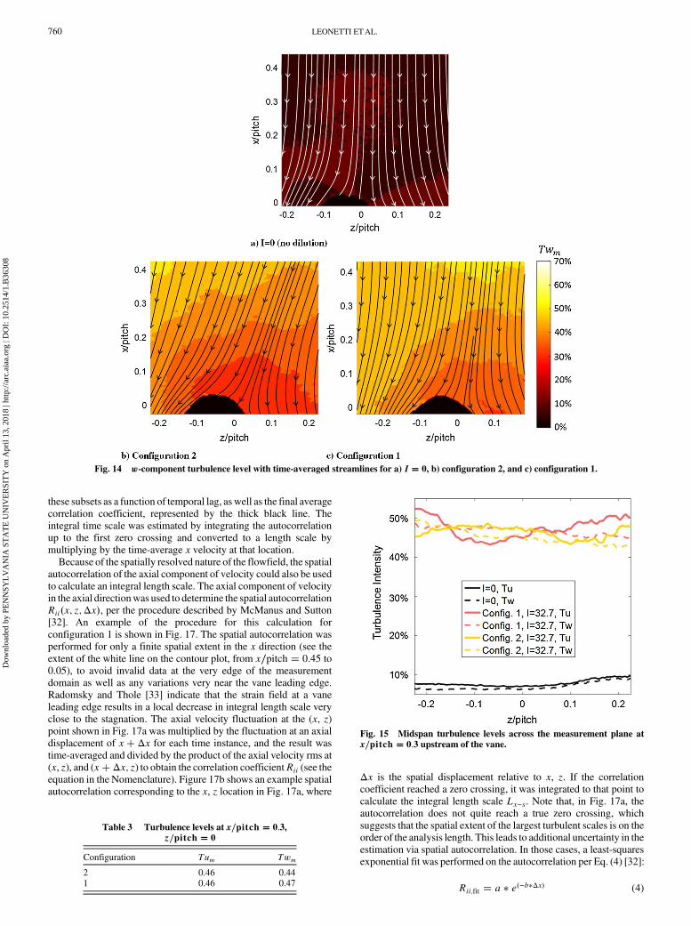
the right (z∕pitch � 0.1), which are associatedwith the high-velocityremnant of the large ID jet described for Fig. 9.The fluctuating w-velocity component was also obtained in this

study. Relative to many turbine inflow turbulence studies that use

single-component hot wires, this pitchwise fluctuation component is

unique and gives some indication of the anisotropy of the turbulence

entering the turbine. Figure 14 shows w-component turbulence

levels, based on mass-averaged turbine inlet velocity, for both

clockings. As indicated in the figure, turbulence levels based on

fluctuatingw-velocity are also larger than 40% upstream of the vane.

Comparing between Figs. 12 and 14, configuration 2 shows some

similarities in the u- and w-turbulence levels upstream of the vane.

However, closer to the vane leading edge, the w-component

turbulence level is reduced relative to the u-component level,

suggesting that the turbulence becomes more anisotropic near the

vane. The configuration 1 clocking shows less satisfactory agreement

between the axial and pitchwise turbulence levels throughout the

measurement plane. This is likely due to the anisotropy of turbulence

in the near wake of the large ID dilution jet near this location. Table 3

shows the u- andw-component turbulence levels at a point upstream

of the vane (x∕pitch � 0.3, z∕pitch � 0) for both clocking cases. Atthis reference location, both cases generate similar levels of

turbulence for the two components measured.Axial (u component) and pitchwise (w component) turbulence

levels were extracted as a function of pitchwise direction across the

measurement window at x∕pitch � 0.3. The results are shown in

Fig. 15 for the two clockings and two turbulence components, as well

as for the no-dilution case (I � 0). Although there are some

differences between the two clockings studied, specifically slightly

more variability in turbulence level for configuration 1 relative to

configuration 2, the overall turbulence levels at this location do not

indicate that clocking had a significant impact on turbulence level.

The turbulence is generated by the breakdown of the dilution jet

coherent structures, which happens relatively independently of the

position of the jets relative to the turbine vanes.Turbulent integral length scaleswere calculated from the high-speed

PIV data set by performing both temporal and spatial autocorrelations.

Fig. 11 Temporal variation of the pitchwise-averaged inlet flow angle at x∕pitch � 0.3 upstream of the vane.

758 LEONETTI ETAL.

Dow

nloa

ded

by P

EN

NSY

LV

AN

IA S

TA

TE

UN

IVE

RSI

TY

on

Apr

il 13

, 201

8 | h

ttp://

arc.

aiaa

.org

| D

OI:

10.

2514

/1.B

3630

8

Only the axial integral turbulent scales are calculated here, and so only

the axial component of velocity (x-direction velocity) is used in the

autocorrelations. For temporally estimated integral scales, the time

record at each PIV interrogation window is used to calculate the

temporal autocorrelation Rii�x; z;Δt�, and Taylor’s frozen turbulencehypothesis is used to determine an integral length scale Lx−t. This is

performed for each small interrogation region in the PIVmeasurement

plane, producing an integral length scale value for each interrogation

region (generally 128 × 128 regions in the measurement domain).

The procedure to estimate temporal autocorrelations at a point in

the flow is illustrated in Fig. 16, for configuration 1. Figure 16a shows

contours of instantaneous axial velocity fluctuations. A time

sequence of data is extracted from the x, z point indicated by thewhitedot, and an autocorrelation is performed on the time sequence.

To reduce noise in the autocorrelation, the entire time sequence

(3 s, 3000 samples) was broken into multiple subsets, and the

resulting autocorrelation curves from each subset were averaged. The

line plot in Fig. 16b shows the various autocorrelation coefficients of

Fig. 12 Axial turbulence level, with time-averaged streamlines for a) I � 0, b) configuration 2, and c) configuration 1.

Fig. 13 Axial turbulence level normalized by local velocity for a) configuration 2, and b) configuration 1.

LEONETTI ETAL. 759

Dow

nloa

ded

by P

EN

NSY

LV

AN

IA S

TA

TE

UN

IVE

RSI

TY

on

Apr

il 13

, 201

8 | h

ttp://

arc.

aiaa

.org

| D

OI:

10.

2514

/1.B

3630

8

these subsets as a function of temporal lag, aswell as the final average

correlation coefficient, represented by the thick black line. The

integral time scale was estimated by integrating the autocorrelation

up to the first zero crossing and converted to a length scale by

multiplying by the time-average x velocity at that location.Because of the spatially resolved nature of the flowfield, the spatial

autocorrelation of the axial component of velocity could also be used

to calculate an integral length scale. The axial component of velocity

in the axial directionwas used to determine the spatial autocorrelation

Rii�x; z;Δx�, per the procedure described by McManus and Sutton

[32]. An example of the procedure for this calculation for

configuration 1 is shown in Fig. 17. The spatial autocorrelation was

performed for only a finite spatial extent in the x direction (see the

extent of the white line on the contour plot, from x∕pitch � 0.45 to

0.05), to avoid invalid data at the very edge of the measurement

domain as well as any variations very near the vane leading edge.

Radomsky and Thole [33] indicate that the strain field at a vane

leading edge results in a local decrease in integral length scale very

close to the stagnation. The axial velocity fluctuation at the (x, z)point shown in Fig. 17a was multiplied by the fluctuation at an axial

displacement of x� Δx for each time instance, and the result was

time-averaged and divided by the product of the axial velocity rms at

(x, z), and (x� Δx; z) to obtain the correlation coefficientRii (see the

equation in the Nomenclature). Figure 17b shows an example spatial

autocorrelation corresponding to the x, z location in Fig. 17a, where

Δx is the spatial displacement relative to x, z. If the correlation

coefficient reached a zero crossing, it was integrated to that point to

calculate the integral length scale Lx−s. Note that, in Fig. 17a, the

autocorrelation does not quite reach a true zero crossing, which

suggests that the spatial extent of the largest turbulent scales is on the

order of the analysis length. This leads to additional uncertainty in the

estimation via spatial autocorrelation. In those cases, a least-squares

exponential fit was performed on the autocorrelation per Eq. (4) [32]:

Rii;fit � a � e�−b�Δx� (4)

Fig. 14 w-component turbulence level with time-averaged streamlines for a) I � 0, b) configuration 2, and c) configuration 1.

Table 3 Turbulence levels at x∕pitch � 0.3,z∕pitch � 0

Configuration Tum Twm

2 0.46 0.441 0.46 0.47

Fig. 15 Midspan turbulence levels across the measurement plane atx∕pitch � 0.3 upstream of the vane.

760 LEONETTI ETAL.

Dow

nloa

ded

by P

EN

NSY

LV

AN

IA S

TA

TE

UN

IVE

RSI

TY

on

Apr

il 13

, 201

8 | h

ttp://

arc.

aiaa

.org

| D

OI:

10.

2514

/1.B

3630

8

where a and b are fit coefficients. Then, the integral scale Lx−s is the

inverse of the b coefficient. The length scales estimated from an

exponential fit and from integration of the autocorrelation curve

generally agreed well with each other.

Figure 18 shows the variation in the axial integral length scale,

normalized by large jet diameter, across the pitch of the

measurement plane for the two analysis methods described

(temporal autocorrelation and spatial autocorrelation). Note that the

temporal autocorrelation can provide estimates of Lx−t throughout

the entire measurement domain because each PIV interrogation

window provides a time signal, but the spatial autocorrelation is

performed over a finite spatial window in the x direction and thus

can only provide distinct values for Lx−s in the pitchwise direction.

In Fig. 18, Lx−t is evaluated at x∕pitch � 0.45 for comparison to

Lx−s. For a given clocking, the two methods of integral length scale

calculation show somewhat reasonable agreement with each other.

A quantitative comparison of the pitchwise-average length scale at

x∕pitch � 0.45 for configurations 1 and 2 is given in Table 4.

For both cases in Fig. 18, the integral length scale was found to be

on the order of the dilution jet diameter, which is similar to previous

studies (Barringer et al. [7]). There is not a clear trend of length scale

variation with dilution clocking for this study, although the two

configurations seem to be out of phase, which might be expected

from the different dilution hole positions. Note that variation in

integral scales between cases is within the estimated uncertainties of

this quantity.

Fig. 16 Representations of a) instantaneous axial velocity fluctuation, and b) the temporal autocorrelation at the white circle in Fig. 16a.

Fig. 17 Representations of a) instantaneous axial velocity, and b) the spatial autocorrelation for various spatial lags along the white line in Fig. 17a.

Fig. 18 Midspan axial integral length scale using temporal and spatialautocorrelations.

Table 4 Average axial integral length scale at x∕pitch � 0.45

Method Configuration 2 Configuration 1

Temporal autocorrelation: Lx−t∕D 0.40 0.40Spatial autocorrelation: Lx−s∕D 0.38 0.39

LEONETTI ETAL. 761

Dow

nloa

ded

by P

EN

NSY

LV

AN

IA S

TA

TE

UN

IVE

RSI

TY

on

Apr

il 13

, 201

8 | h

ttp://

arc.

aiaa

.org

| D

OI:

10.

2514

/1.B

3630

8

V. Conclusions

Two-dimensional high-speed particle image velocimetry mea-surements at 1 kHz were obtained at the midspan of a turbine vanedownstream of a simulated rich-burn–quench–lean-burn combustor,to study the effects of two dilution hole arrangements. The combustorand vane were representative of commercial aircraft enginegeometries and were scaled up to allow for high measurementresolution. In one dilution hole arrangement (clocking), known asconfiguration 1, a large dilution hole was positioned directlyupstream of the vane leading edge. In the second arrangement(configuration 2), the large dilution hole was shifted away from thevane leading edge. A single dilution momentum flux ratio (as well asa no-dilution case) was studied.Configuration 2 was shown to have a more uniform inlet velocity

profile than configuration 1, although neither was completelyuniform in the pitchwise direction, as is often assumed during turbinedesign. This nonuniformity is believed to be the result of aligning thecenterline of a singular jet with the vane leading edge. Configuration2 had themost extreme negative inlet flow angle; configuration 1 alsohad a negative inlet angle, but not as severe as configuration 2. This isbelieved to be a result of the acceleration of the low-momentumregion behind the large outer diameter jet around the vane suctionside. Turbulence levels for both clockings were similar, as wasexpected. This was true also for both recorded components ofturbulence, suggesting turbulence isotropy upstream of the vane. Thesimilar levels of turbulence are thought to be a result of the turbulentjets mixing with the crossflow before the vane pressure field, andtherefore the clocking effect, acts to distort the flow. This would alsoexplain the similarities in the integral length scale values. Increasinganisotropy between turbulence components near the vane leadingedgewas influenced by the dilution hole clocking, suggesting that thespatial nonuniformity of the combustor exit mean velocity isimportant not only for the time-average vane loading but also for theevolution of the turbulence field in the high-strain region around avane leading edge. The levels of turbulence (∼46%) found in thiscombustor configuration are well above previous studies, whichwould be expected to increase vane leading-edge heat transfer andnegatively impact the performance of the turbine vane.This study suggests that the inlet conditions to the turbine for

certain combustor types may be more turbulent than previouslythought but also that the high-momentum dilution jets result in anonuniform velocity profile that can persist into the turbine.Turbulence levels and integral length scales estimated in thisexperiment could be used in the correlations available in literature topredict heat transfer augmentation on a first vane. These correlations,however, do not take into account nonuniform velocity distributionsupstream of the vane. Clearly, it is important to consider the spatiallyand temporally resolved influence of the combustor exit flow on thefirst vane in the quest to improve gas turbine efficiency and reliability.Future studies should investigate the relationship between thedilution hole placement in both the pitchwise and streamwisedirections relative to the turbine vanes and providemore details of thespatial distribution of velocity, turbulence, and integral length scalesentering the turbine.

Acknowledgment

The authors would like to thank United Technologies — Pratt &Whitney for their financial and technical support of this work.

References

[1] Fric, T. F., and Roshko, A., “Vortical Structure in the Wakeof a Transverse Jet,” Journal of Fluid Mechanics, Vol. 279, Nov. 1994,pp. 1–47.doi:10.1017/S0022112094003800

[2] Holdeman, J. D., “Mixing of Multiple Jets with a Confined SubsonicCrossflow,” Progress in Energy and Combustion Science, Vol. 19,No. 1, 1993, pp. 31–70.doi:10.1016/0360-1285(93)90021-6

[3] Holdeman, J. D., Liscinsky, D. S., and Bain, D. B., “Mixing of MultipleJets with a Confined Subsonic Crossflow: Part 2—Opposed Rows of

Orifices in Rectangular Ducts,” Journal of Engineering for Gas

Turbines and Power, Vol. 121, No. 3, 1999, pp. 551–562.doi:10.1115/1.2818508

[4] Holdeman, J. D., Srinivasant, R., and Berenfeld, A., “Experimentsin Dilution Jet Mixing,” AIAA Journal, Vol. 22, No. 10, 1984,pp. 1436–1443.doi:10.2514/3.48582

[5] Cha, C. M., Ireland, P. T., Denman, P. A., and Savarianandam, V.,“Turbulence Levels Are High at the Combustor–Turbine Interface,”Proceedings of the ASME Turbo Expo 2012: Turbine Technical

Conference and Exposition, ASME Paper GT2012-69130, New York,2012, pp. 1371–1390.doi:10.1115/GT2012-69130

[6] Vakil, S. S., and Thole, K. A., “Flow and Thermal Field Measurementsin a Combustor Simulator Relevant to a Gas Turbine Aeroengine,”Journal of Engineering for Gas Turbines and Power, Vol. 127, No. 2,2005, pp. 257–267.doi:10.1115/1.1806455

[7] Barringer, M. D., Richard, O. T., Walter, J. P., Stitzel, S. M., and Thole,K.A., “FlowField Simulations of aGas TurbineCombustor,” Journal ofTurbomachinery, Vol. 124, No. 3, 2002, pp. 508–516.doi:10.1115/1.1475742

[8] Ames, F. E., andMoffat, R. J., “Heat Transfer withHigh Intensity, LargeScale Turbulence: The Flat Plate Turbulent Boundary Layer and theCylindrical StagnationPoint,”StanfordUniv., Rept. HMT-44, Stanford,CA, 1990.

[9] Ames, F. E., “The Influence of Large-Scale High-Intensity Turbulenceon Vane Heat Transfer,” Journal of Turbomachinery, Vol. 119, No. 1,1997, pp. 23–30.doi:10.1115/1.2841007

[10] Gandavarapu, P., and Ames, F. E., “The Influence of Leading EdgeDiameter on Stagnation Region Heat Transfer Augmentation IncludingEffects of Turbulence Level, Scale, and Reynolds Number,” Journal ofTurbomachinery, Vol. 135, No. 1, 2012, Paper 011008.doi:10.1115/1.4006396

[11] Ames, F. E., “Aspects of Vane Film Cooling with High Turbulence: Part2—Adiabatic Effectiveness,” Journal of Turbomachinery, Vol. 120,No. 4, 1998, pp. 777–784.doi:10.1115/1.2841789

[12] Nasir, S., Carullo, J. S., Ng, W.-F., Thole, K. A., Wu, H., Zhang, L. J., andMoon,H.K., “Effects of Large ScaleHighFreestreamTurbulence andExitReynoldsNumber onTurbineVaneHeat Transfer in a TransonicCascade,”Journal of Turbomachinery, Vol. 131, No. 2, 2009, Paper 021021.doi:10.1115/1.2952381

[13] Radomsky, R. W., and Thole, K. A., “Detailed Boundary LayerMeasurements on aTurbineStatorVane at Elevated FreestreamTurbulenceLevels,” Journal of Turbomachinery, Vol. 124, No. 1, 2001, pp. 107–118.doi:10.1115/1.1424891

[14] Van Fossen, G. J., Simoneau, R. J., and Ching, C. Y., “Influence ofTurbulence Parameters, Reynolds Number, and Body Shape onStagnation-Region Heat Transfer,” Journal of Heat Transfer, Vol. 117,No. 3, 1995, pp. 597–603.doi:10.1115/1.2822619

[15] Cha, C.M., Hong, S., Ireland, P. T., Denman, P., and Savarianandam,V.,“Experimental and Numerical Investigation of Combustor–TurbineInteraction Using an Isothermal, Nonreacting Tracer,” Journal of

Engineering for Gas Turbines and Power, Vol. 134, No. 8, 2012,Paper 081501.doi:10.1115/1.4005815

[16] Salvadori, S., Riccio, G., Insinna, M., and Martelli, F., “Analysis ofCombustor/Vane Interaction with Decoupled and Loosely CoupledApproaches,” Proceedings of the ASME Turbo Expo 2012: Turbine

Technical Conference and Exposition, ASME Paper GT2012-69038,New York, 2012, pp. 2641–2652.doi:10.1115/GT2012-69038

[17] Stitzel, S., and Thole, K. A., “Flow Field Computations of Combustor–Turbine Interactions Relevant to a Gas Turbine Engine,” Journal of

Turbomachinery, Vol. 126, No. 1, 2004, pp. 122–129.doi:10.1115/1.1625691

[18] Insinna, M., Salvadori, S., and Martelli, F., “Simulation of Combustor/NGV Interaction Using Coupled RANS Solvers: Validation andApplication to a Realistic Test Case,” Proceedings of the ASME Turbo

Expo 2014: Turbine Technical Conference and Exposition, ASMEPaper GT2014-25433, New York, 2014, Paper V02CT38A010.doi:10.1115/GT2014-25433

[19] Prenter, R., Ameri, A., and Bons, J. P., “Measurement and Prediction ofHot Streak Profiles Generated by Axially Opposed Dilution Jets,” 53rdAIAA Aerospace Sciences Meeting, AIAA Paper 2015-0304, 2015.doi:10.2514/6.2015-0304

762 LEONETTI ETAL.

Dow

nloa

ded

by P

EN

NSY

LV

AN

IA S

TA

TE

UN

IVE

RSI

TY

on

Apr

il 13

, 201

8 | h

ttp://

arc.

aiaa

.org

| D

OI:

10.

2514

/1.B

3630

8

[20] Gibson, J., Thole, K., Christophel, J., and Memory, C., “Effects of theMain Gas Path Pressure Field on Rim Seal Flows in a Stationary LinearCascade,” Proceedings of the ASME Turbo Expo 2015: Turbine

Technical Conf. and Exposition, ASME Paper GT2015-43517, NewYork, 2015, Paper V05CT15A029.doi:10.1115/GT2015-43517

[21] Perdichizzi, A., “Mach Number Effects on Secondary FlowDevelopment Downstream of a Turbine Cascade,” Journal of

Turbomachinery, Vol. 112, No. 4, 1990, pp. 643–651.doi:10.1115/1.2927705

[22] Hermanson, K. S., and Thole, K. A., “Effect of Mach Number onSecondary Flow Characteristics,” International Journal of Turbo and

Jet Engines, Vol. 17, No. 3, 2000, pp. 179–196.doi:10.1515/TJJ.2000.17.3.179

[23] Nealy, D. A., Gladden, H. J., Mihelc, M. S., and Hylton, L. D.,“Measurements of Heat Transfer Distribution over the Surfaces ofHighly Loaded Turbine Nozzle Guide Vanes,” Journal of Engineeringfor Gas Turbines and Power, Vol. 106, No. 1, 1984, pp. 149–158.doi:10.1115/1.3239528

[24] Arts, T., and De Rouvroit, M. L., “Aero-Thermal Performance of aTwo Dimensional Highly Loaded Transonic Turbine Nozzle GuideVane: A Test Case for Inviscid and Viscous Flow Computations,”Proceedings of the ASME 1990 International Gas Turbine and

Aeroengine Congress and Exposition, ASME Paper 90-GT-358,New York, 1990, Paper V001T01A106.doi:10.1115/90-GT-358

[25] Nix, A. C., Diller, T. E., and Ng, W. F., “Experimental Measurements andModeling of the Effects of Large-Scale Freestream Turbulence on HeatTransfer,” Journal of Turbomachinery, Vol. 129,No. 3, 2007, pp. 542–550.doi:10.1115/1.2515555

[26] Barringer, M. D., Polanka, M. D., and Thole, K. A., “Effects ofCombustor Exit Profiles on Vane Aerodynamic Loading and HeatTransfer in a High Pressure Turbine,” Journal of Turbomachinery,

Vol. 131, No. 2, 2009, Paper 021008.doi:10.1115/1.2950051

[27] Zimmerman, D. R., “Laser Anemometer Measurements at the Exit of aT-63-C20 Combustor,” NASA Rept. ADA072709, 1979.

[28] Moss, R., and Oldfield, M., “Measurements of Hot CombustorTurbulence Spectra,” Proceedings of the ASME 1991 International Gas

Turbine and Aeroengine Congress and Exposition, ASME Paper 91-GT-351, New York, 1991, Paper V004T09A025.doi:10.1115/91-GT-351

[29] Moffat, R. J., “Describing the Uncertainties in ExperimentalResults,” Experimental Thermal and Fluid Science, Vol. 1, No. 1,1988, pp. 3–17.doi:10.1016/0894-1777(88)90043-X

[30] Wieneke, B., “Generic A-Posteriori Uncertainty Quantification for PIVVector Fields by Correlation Statistics,” Proceedings of the 17th

International Symposium on Applications of Laser Techniques to Fluid

Mechanics, 2014.[31] Roach, P. E., “TheGeneration of Nearly Isotropic Turbulence byMeans

of Grids,” International Journal of Heat and Fluid Flow, Vol. 8, No. 2,1987, pp. 82–92.doi:10.1016/0142-727X(87)90001-4

[32] McManus,T.A., andSutton, J.A., “LargeScaleDynamics andStatisticsof the Time-Varying Temperature Field in Turbulent Non-Premixed JetFlames,” 53rd AIAA Aerospace Sciences Meeting, AIAA SciTech

Forum, AIAA Paper 2015-0671, 2015.doi:10.2514/6.2015-0671

[33] Radomsky, R. W., and Thole, K. A., “Flowfield Measurements fora Highly Turbulent Flow in a Stator Vane Passage,” Journal of

Turbomachinery, Vol. 122, No. 2, 2000, pp. 255–262.doi:10.1115/1.555442

K. FrendiAssociate Editor

LEONETTI ETAL. 763

Dow

nloa

ded

by P

EN

NSY

LV

AN

IA S

TA

TE

UN

IVE

RSI

TY

on

Apr

il 13

, 201

8 | h

ttp://

arc.

aiaa

.org

| D

OI:

10.

2514

/1.B

3630

8