1

Combining regional approach and data extension procedure forassessing GEV distribution of extreme precipitation in Belgium.

Daniel Gellens Royal Meteorological Institute of Belgium, Avenue Circulaire, 3, B-1180, Brussels, Belgium

tel: +(int) 32 2 3730677e-mail: D.Gellens@oma.be

keywords: extreme precipitation, GEV distribution, regionalisation, data extension, L-moments

Abstract

The k-day extreme precipitation depths (k=1, 2, 3, 4, 5, 7, 10, 15, 20, 25 and 30) at the climatologicalnetwork of Belgium (165 stations) are analysed to assess the regional GEV growth curves and todetermine the at-site fractiles. The calendar year and the hydrological summer and winter areconsidered separately. The method proposed combines regional L-moment estimates of the GEVparameters and tends to take advantage of a few long-term well-documented series. Therefore, a dataextension procedure based on the fractiles method has been used to extend the 1951-1995 observationperiod to the 1910-1995 reference period. This ensures the temporal homogeneity of the series byassessing the possible missing extremes and it places all the series in a reference period where thestationarity of the extreme precipitation has been verified. Using the 9 historical series and generatingrandomly located missing values the efficiency of three data extension methods has been evaluated.This comparison indicates that a procedure using the regional growth curve satisfies this task. It showsthat the residual mean square error of the at-site means is reduced when the mean correlation betweenthe reference station and the series presenting gaps exceeds 0.52 but that the corresponding error onhigh order fractiles is reduced for all the observed correlation and for large numbers (40-50) of missingvalues. A practical estimation of the confidence intervals is proposed.

Introduction

The distributions of the k-day extreme precipitation depths are of great interest since their knowledgeis very important in many practical domains ranging from the building of rain collectors, drainagesystems to river control. In addition to this prior knowledge of high precipitation rates in order to preventhydrological systems to be overloaded, one of the tasks of the Royal Meteorological Institute of Belgiumis to assess a posteriori the regions where some rain events can be considered as exceptional. This kindof study required by the Federal Government can be followed by the use of specific funds to help thepopulation to repair the disaster in the cases where insurance companies refuse to pay damages notcompletely covered by their contracts.

In this framework, the present study follows several studies carried out in Belgium in order to improvethe estimation of the fractiles of the extreme k-day precipitation depths. These studies were at firstcentred on the long-term series of the reference station Uccle (Sneyers, 1961, 1977 and 1979; Buishandand Demarée, 1990). Dupriez and Demarée (1988 and 1989) start to study the regional distribution ofthe extreme precipitation depths essentially by taking the stations individually, i.e. independently, andproducing maps of fractiles. The present study tends to use the links between the stations and to takeadvantage of the existence of a few well-documented long-term series. These stations can be usefulin order to improve the estimates of the statistical distributions of the extremes. This study exploits thewell-established regional approach based on the Probability Weighted Moments (PWM) developedinitially by e.g. Greenwood et al. (1979) and Hosking et al. (1985) and will combine it with the dataextension procedure, a method usually used to assess missing values of data records.

In the first chapter, the data sets used are described. The statistical homogeneity of the extreme series

2

is then verified by means of regional tools. This allows to consider the whole 165 stations as ahomogeneous region and to assess the GEV distributions at the regional scale. After a summary of theregionalisation technic, the data extension procedure is described and its efficiency verified. The GEVdistribution parameters obtained by means of the combined procedure are then presented. Theconstruction of the confidence intervals requires some more comments which leads to the establishmentof the fractiles and their confidence intervals for any station of the studied area.

Data set presentation

Daily precipitation amounts of the Belgian climatological network are available on magnetic media fora period starting merely in 1951. They have been studied here until 1995, i.e. for a 45-year period. Thesummation of these daily values over a period of k days provides k-day precipitation. The annualmaximum values have been identified, this means the maximum values corresponding to the calendaryear and the extreme values of the hydrological winter and summer. These two separate 6-month sub-periods are starting respectively at the 1 of October and at the 1 of April. They allow the separation,st st

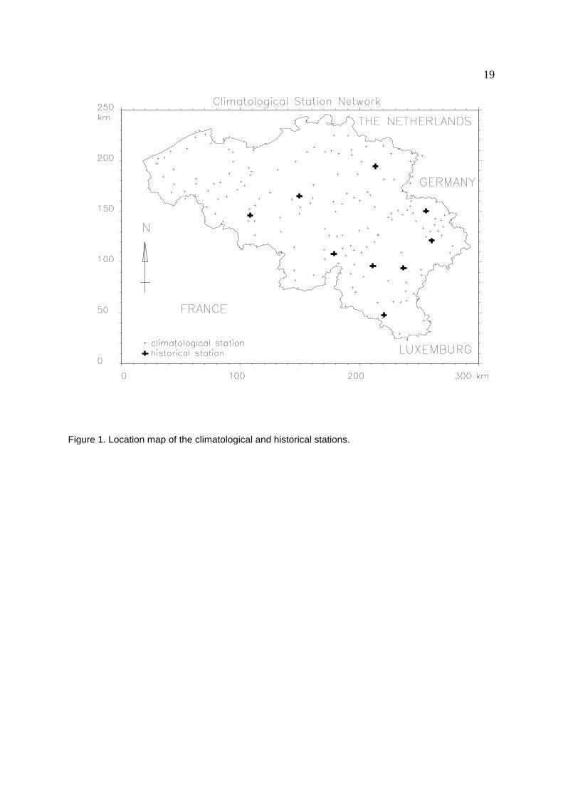
at least for small k, of the mainly convective events observed in summer from the predominantly frontalprecipitation events in winter. After rejection of stations presenting more than 6 missing yearly values,a set of 165 stations remained, i.e. on average about one station per 200 km . Figure 1 shows their2

location and their rather homogeneous distribution over the country.

The k-day extreme values have been studied for k=1, 2, 3, 4, 5, 7, 10, 15, 20, 25 and 30, for the threeabove-mentioned periods of the year. Longer data records are also available but only for a few stations.In these cases, the data sets start around 1880, the year of the foundation of the meteorological network.Bold crosses indicate the locations of these stations in figure 1. Only 9 long-term stations have beenmade available in a first stage by Bultot and its collaborators (Bultot and Dupriez, 1976; Dupriez andDemarée, 1988). They were finalized by Demarée in the framework of the NACD project (North AtlanticClimate Data, Frich et al., 1996). For instrumental, network and also possibly climatological reasons,only data after 1910 are instrumentally homogeneous and can be used for studying the extremeprecipitation distribution.

Regional homogeneity of the distributions

As shown in Gellens (2000) the extremes for each period of the year and each k value are presentinga strong spatial correlation. This correlation is obviously stronger for the winter extremes than for thesummer values and grows with growing k. For k greater than 7 in winter the correlation betweenextremes remains significant for distances greater than 200 km, this means something like the size ofthe studied area. This feature indicates that extreme series must be considered in some way at theregional scale.

Therefore before applying any regional approach, it is at first needed to verify the distributions of theextremes of all the stations for a given k and a given period of the year can be considered as identical.Two homogeneity tests developed by Hosking and Wallis (1993, 1997) were thus used. These tests arebased on the study of the dispersion of the L-moments and in particular of the L-CV, the coefficient ofvariation assessed by means of the L-moments, and of the L-skew and L-kurtosis.

L-moments estimators can be constructed by means of the PWM estimators. For the station j belongingto the n=165 stations of the climatological network, the order r PWM, � , can be defined as (Greenwoodrjet al., 1979)

� = E[ y [F(y)] ] with j=1, ..., nrj j j jr

where F is the cumulative distribution function of y, the observation at station j. For simplicity, the k indexj jindicating the aggregation step has been omitted. The L-moments are linear combinations of the PWMs.The four first L moments are

� = � = µ � = 2� -� � = 6� -6� +� � = 20� -30� +12� -�1j 0j j 2j 1j 0j 3j 2j -j 0j 4j 3j 2j 1j 0j

brj�1nj�nj

i�1

(i�1)(i�2)...(i�r)(nj�1)(nj�2)...(nj�r)

y(i)j

y(1)j y(2)j y(nj�1)j y(nj)j

t R��

n

j�1nj tj /�

n

j�1nj t R

l ��n

j�1nj tlj /�

n

j�1nj

V� �n

j�1nj (tj� t R)2 /�

n

j�1nj

H�

V�µV

�V

V3��n

j�1nj (t3j� t R

3 )2� (t4j� t R

4 )2 /�n

j�1nj

3

(where µ is the mean) and the L moments ratios are the L-CV = � = � /� , the L-skew = � = � /� andj j 2j 1j 3j 3j 2jthe L-kurtosis = � = � /�4j 4j 2j

Unbiased estimators of � are assessed by (Landwehr et al., 1979)rj

where n is the number extremes considered for station j and y are the ordered observations y so thatj (i)j j� � ... � � . Regional average L moments ratios t , t and t are defined asR R R

3 4

and with l=3,4 (1)

where t , t and t are the estimators of � , � and � .j 3j 4j j 3j 4j

Hosking and Wallis (1993) introduced two measures of the dispersion of the L moments ratios aroundtheir regional average values. They defined

and fit a kappa distribution having moments equal to the regional L moments ratios t , t and t in orderR R R3 4

to simulate a large number (500 in the present case) of regions with n stations having the same numberof values and the same distribution. For each of these regions the statistic V is assessed and their meanµ and standard deviation � are used to determine the heterogeneity measure H asV V

They suggest that the region be considered as “acceptably homogeneous” if H<1, “possiblyheterogeneous” if 1�H<2 and “definitely heterogeneous” if H�2. These authors also introduced a secondmeasure V based on t and t3 3 4

R R

and defined H accordingly with V .3 3

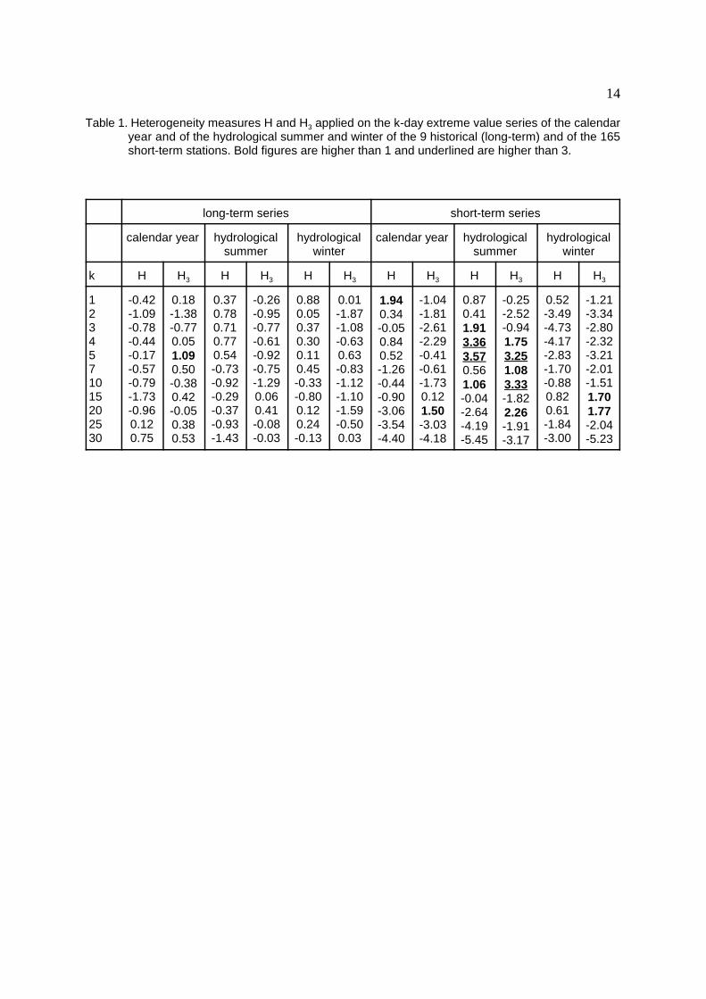
These homogeneity measures have been applied on the data sets and the results are given in table 1.For most of the k values and periods of the year, the H and H statistics are smaller than 1. This confirms3the homogeneity of the data distributions. For the summer season, some k values are howevercharacterised by higher figures (for k equal to 4 and 5 for H, and for k equal to 5 and 10 for H ). As these3higher values are only detected for two k values among the large number of studied cases, they werenot taken into consideration to justify a clustering procedure of the data set into smaller homogeneousarea. The same two tests applied on the historical data give only values smaller than 1 and indicate thestatistical homogeneity of the 9 long-term series. It is interesting to note that large negative values of Hand H can be found in table 1, in particular for the tests applied on the short-term series. According to3Hosking and Wallis (1997) these values are indicating that “there is a strong cross-correlation betweenthe site’ frequency distribution or that there is an excessive regularity in the data that causes the L-CVsto be unusually close together”. In the present case these results are in consequence not surprising dueto the high density of the climatological network and the correlation between the rainfall events. It is

( � , � , � )T

�R

�R�7.8590c � 2.9554c 2 c� 2

3� t R3

�

ln2ln3

�R�

�2�R

(1�2��R)�(1� �R)

�R��1� �

R[1��(1� �R)] /�R

� (x)��

�

0

t x�1e �tdt �1�1 �2� t R

4

indeed this general characteristic of the rainfall that will be exploited here.

Regional estimates of the GEV growth curves

In regional frequency analysis, data from different stations are combined to assess the unknownparameters of a given distribution in a more efficient way. Several procedures exist and the comparisoncarried out by Cunnane (1988) can be mentioned to shown the diversity of the methods. In the presentstudy the so-called index flood method based on standardized PWMs has been implemented. Itsupposes (Hosking and Wallis, 1997) the Q(F) fractile function for the station j be determined by thejproduct

Q(F) = µ q(F), 0<F<1 (2)j j

of the at-site mean µ and q(F) the regional dimensionless growth curve common to all the stations. Thisjmethod supposes that the stations form a homogeneous region, i.e. that the frequency distributions arethe same apart from a scaling factor. Distributions of the extreme precipitation amounts are usuallydescribed by the GEV (General Extreme Value) distribution (Jenkinson, 1969, 1977). This choice istheoretically and practically justified (Cong et al., 1993, Stedinger et al., 1993).

The GEV distribution function is

F(x) = exp [ -{1 - � (x-�)/�} ] for � � 01/�

where � and � are the location and scale parameters, and � the shape parameter. The GEV distributionreduces to the Gumbel distribution for �=0: F(x) = exp [ - exp { -(x-�)/�} ] =G(x). The three parameters(�, �, �) are assessed by the PWM method (Hosking et al., 1985). Equating the three first theoreticalT

moments with their estimated values equal to 1, t and t in the regional framework gives a system ofR R3

three equations and their estimates . The regional mean is unit as the data have been scaledby their means and the regional L-CV t and L-skew t have been defined just above. Routines usedR R

3in the present study are those provided by Hosking (1997).

The growth curve is the inverse of F and is given by

q(F) = � + � {1-(-ln F) }/� for � � 0, 0<F<1�

It is thus a function of the three first regional L moments ratios. Hosking et al. (1985) established thePWMs estimators of the GEV parameters. They proposed an approximation for shape parametersbelonging to the interval (-1/2,1/2) that provides here the estimator of the regional shape parameter

with .

It shows the shape depends only on the regional L-skew,

and

(3)

where � (.) is the gamma function given by and where and .

In the particular case of the growth curve we have therefore according to (3) that

�R�1� �R[1��(1� �R)] /�R

qR(F)�1� �R[�(1� �R)� (� lnF)�R] /�R

yr,giyj,gi

yj,gi�F �1

j {Fr{yr,gi} }

5

and hence

(4)

that depends only on two parameters.

Data extension procedure et verification of its efficiency

As mentioned in the data set description the reference period of most of the data is 1951-1995. Theselection of the extreme series described just before allows nevertheless some stations to present a fewmissing extreme values. Therefore, the records of all the stations are not covering all the same years.It has been shown in a preliminary analysis of the extreme values on Belgium (Gellens, 1995) that thistemporal inhomogeneity can have in some particular cases a strong impact on the fractile assessment.It is particularly salient in the south of Belgium when the precipitation events corresponding to the floodsof December 1993 and January 1995 are not included in the data of a station and are present for theneighbouring stations. Long-term fractiles are then evolving in different ways according to the existenceor not of this data in the observations. It has been shown that assessing missing extreme observationsof this particular station could restore the homogeneity of the data and could correct the evolution of thefractiles at that location. This problem has been tested for the short-term stations close to the stationspresenting missing values (Gellens, 1998). It provides a first argument for assessing the missing valuesof the extreme k-day series by means of the observations of the complete reference stations.

On the short 1951-1995 reference period, the study of the stationarity of the extreme precipitationamounts (Gellens, 2000) has shown significant trends in winter extreme k-day precipitation for all thevalues of k. No significant trend has been found in extreme summer precipitation. Annual extremedepths show no trends for small k, as summer events dominate, and significant trends for k larger than7 due to winter events. The analysis of the 9 long-term series showed no significant trend for the period1910-1995, but these series also reproduce almost the same trends as those found for the majority ofthe stations for the shorter 1951-1995 period. This second result also advocates for the use of the dataextension procedure to place the study of the extreme values in a framework granting the stationarityof the studied series.

For the two reasons mentioned above, it has been decided to combine the data extension approach tothe regional procedure for distribution fitting. But before any action, it is at first needed to verify theefficiency of the data extension procedure. In particular, does the data extension procedure reduce aftercompletion the at-site standard error of the extreme k-day precipitation mean which is the first factor ofthe expression (2). It will be also interesting to verify if the standard error of the long-term fractiles isaccordingly reduced. The first condition is probably the most important in regional approach as the at-site mean is used to scale the observation sets and get the same distribution on all the area. The secondone could be interesting as the shape factor of the regional distribution will depend on the highest fractileestimates.

The fractile method consists in supposing the missing values in the record of station j, y arej,corresponding to the same fractiles as the observations at a reference station r for the same year. Theparameters of two distributions are therefore estimated by the PWM method on the data of the commonyears of the two series, i.e. respectively the cumulative distribution function F and F . Let’s define n’ asj rthe number of missing extreme values in the record of the station j and g the year of these missingiextreme values, with i=1, ... n’. The n’ fractile values at the reference station corresponding to the gaps,i.e. the observed extremes are then used to assess the n’ missing values . Their values are givenby

for i=1, ... n’ (5)

The efficiency of the fractile method and hence of the data extension procedure will obviously depend

yj,gi�

µj

µr

yr,gi

yj,gi�

�j

�r

(yr,gi� �r )� �j

yj,gi

6

on the choice of the F distribution. Therefore different distributions will be tested. At first it is possible touse the regional growth curve q(F) introduced in (2) although the parameters of this growth curve areunknown. The Gumbel distribution and finally the GEV distribution will also be compared with.

In the case of the unknown regional growth curve common to all the stations and thus to the twosamples the expression (5) reduces to a very simple expression

for i=1, ... n’

where µ and µ are respectively the means of the station j and of the reference station r on the sub-r jsample.

For the Gumbel distribution the expression (5) corresponds in fact to a linear relationship

for i=1, ... n’

where � , � , � and � are respectively the location and scale parameters of the station j and of ther j r jreference station r.

The verification protocol has been constructed by means of the long-term series. This avoids buildingthe method on some assumption dealing with the identification of the data distribution law. For a givenk and for the hydrological winter and summer, n’ randomly located gaps have been substituted to theexisting data , i=1, ...n’. By means of the study of the correlation between the series, the mostcorrelated station y is selected as reference station. r

A comparison between the original mean and fractiles with those obtained after data completion can becarried out. Values of n’ equal to 1, 5, 10, 20, 30, 40 and 50 have been considered and k=1, 3, 10 and30. In each case 1000 sets of missing values have been built (except for n’=1 where all the missingvalues can be exhaustively generated) for the 9 historical stations series. The fractiles are assessed bymeans of a GEV distribution fitted on the reconstructed data using PWMs method. They are comparedwith the fractile values estimated directly on the data without gaps completion. Residual mean errors ofestimation are calculated by means of the unbiased Jackknife estimates of the means and of thefractiles. The comparison of these four residual mean errors (rms) indicates if it is interesting to assessthe missing values or not, i.e. if it reduces the rms of the estimates and the most appropriate method todo it. As reference, the mean correlation between the series with gaps and their reference series arealso reproduced to identify the required mean correlation to get a rms reduction.

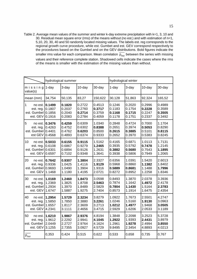
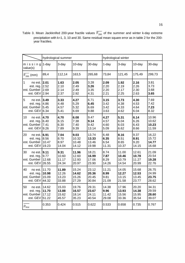
Table 2 and 3 show respectively the residual mean error on the mean and on the 200-year fractiles.When the mean correlation is higher or equal than 0.52 it appears that the mean estimates are improvedby the data extension procedure whatever the number of gaps generated (from 1 to 50). This is not thecase for long-term fractile estimates. For a small number of gaps in the data, there is merely anenhancement of the fractile estimates for very high mean correlation (higher than 0.70). When some 30missing values are generated the data extension procedure gives an improvement of the fractileassessment for a mean correlation higher than 0.52 and for more than 40 gaps the data extensionimproves almost all the fractile estimates. Now if we compare the three fractiles methods, it is obviousthat the GEV based method performs poorly. The main reason is that some instabilities in the shapeparameters are occurring when small samples are used for fitting the three GEV parameters and henceestimating the fractiles of the missing values. The method based on the Gumbel and the one based onthe regional growth curve are almost equally good as concerns the mean estimates and the results givenin table 2 for large number of gaps are not discriminating clearly the two procedures. The resultsconcerning the fractile estimates yielded in table 3 are advocating for the growth curve method providingan improvement of the fractiles for almost all the correlation level for 40 and 50 gaps. In addition it givesmore coherence in the procedure than adopting a robust Gumbel distribution to assess data distributedaccording to GEV distributions.

var �QT� �var �µ qT� � µ2�var �qT ��var � µ � � (E � qT �)2

�2µ�E � qT � �covar � µ ,qT �

E � qT � � qT� ���

�(1�K �

T )

7

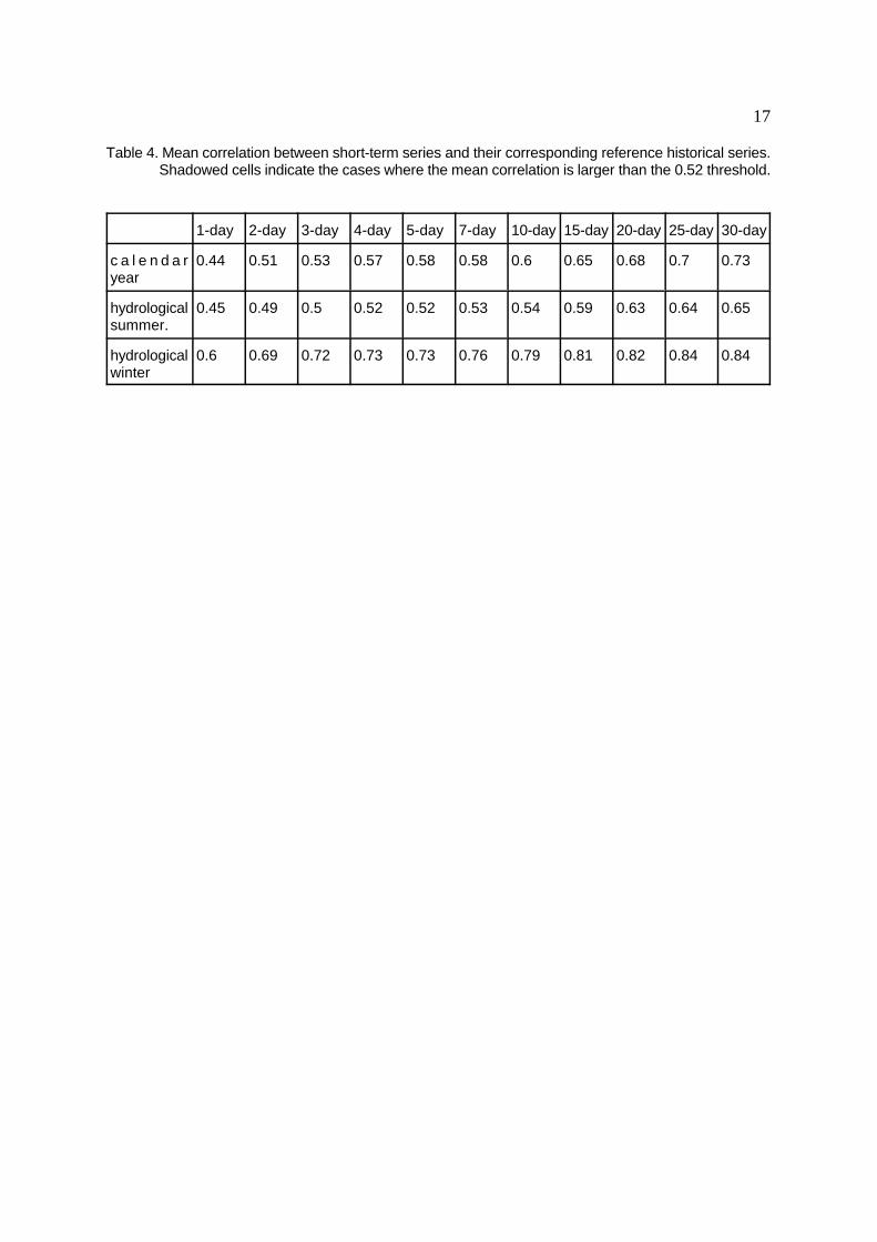
As concerns the 165 short-term series the mean correlation between historical and short-term series isslightly higher due to the denser network. As shown in Table 4 it reaches the 0.52 threshold for almostall the k values in winter and summer, except for k=1,2 and 3 in summer and k=1 and 2 for the calendaryear. For these five particular cases, the data extension procedure has however been implemented asit enhances the estimates of the fractiles in a efficient way and only reduces slightly the efficience of themean estimates.

Practical results

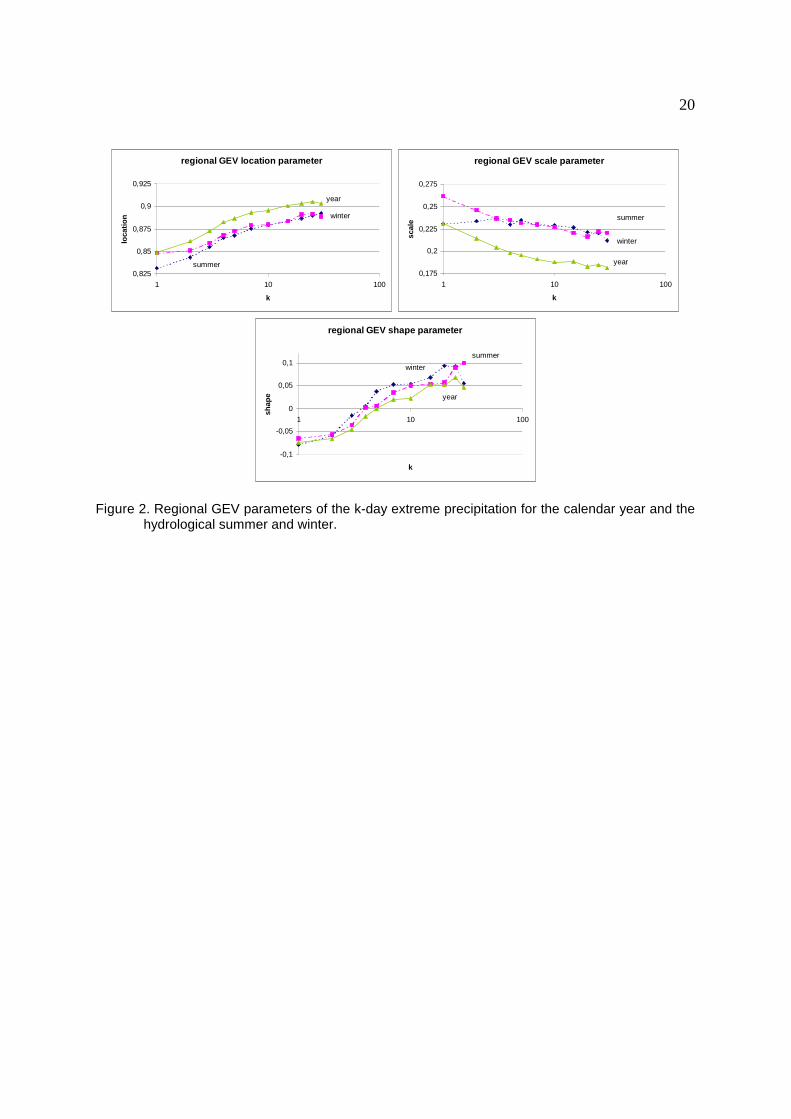
According to the efficiency tests the data extension procedure based on the regional growth curve hasbeen applied on all the k-day extreme precipitation and combined with the regionalisation of thedistribution parameters. The values of the parameters of the GEV regional growth curves are presentedin Figure 2. Due to the reduction of the distribution to a dimensionless curve, all the growth curves andtheir parameters can be easily compared. The parameters from the three periods of the year are fairlyclose to each other in particular as concerns the shape parameter. For most of the k values the locationand scale parameters of the winter and of the summer are almost the same while the calendar yearparameters are respectively slightly higher and lower.

In addition, these pictures show that the parameters are smoothly progressing for one k value to the nextone. The shape parameter show a clear evolution from negative values for the small k values to positivevalues for k values larger than 5. Reducing the confidence interval of the shape parameter, this resultis in agreement with those presented by Buishand (1991) for The Netherlands and initial results fromDupriez et Demarée (1988) but is in contradiction with other studies of Belgian rainfall (e.g. Demarée,1985, Buishand and Demarée, 1990 or Delbeke, 2001). These studies are processing the stationsindividually and the value �=0 provides in this case an interesting simplification for establishing Intensity-Duration-Frequency curves.

The regional approach adopted here confirms the change of the sign of the shape that governs theasymptotic behaviour of the GEV distribution of the k-day extreme precipitation. For a negative shapeparameter the domain is positively unbounded whereas it is bounded for a positive shape parameter.This means the fractiles of very long return periods corresponding to small k values will exceed thosecorresponding to the larger k, a phenomenon that is not physically possible and indicates that therecould be some tail characteristics not captured by the GEV distribution. The return period correspondingto this physical incoherence is nevertheless very long and the confidence interval of the fractiles mustbe taken into consideration. Obviously adopting �=0 would solve this problem but this too restrictivehypothesis has not been adopted here.

Confidence intervals

The estimation of the confidence can be made by following Hosking et al. (1985), Lu and Stedinger(1992a and b) and Rosbjerg and Madsen (1995). The first order development of the expression (2) givesthe variance of the fractile estimate corresponding to a T-year return period (with T = 1 / (1-F) )

(6)

The index j related to the station and the exponent R related to the regional variables have been omittedin this expression. The mean and the variance of the T-year fractile estimator are approximately(Rosbjerg and Madsen, 1995)

(7)

var � qT � ��qT

��

2var���� �qT

��

2var���� �qT

��

2var����

2�qT

��

�qT

��covar��,���2

�qT

��

�qT

��covar��,���2

�qT

��

�qT

��covar��,��

�

�2

n �

�w11�A[Aw22�2w12]�B[Bw33�2w13�2Aw23] �

A �

1�

(1�K �

T )

B �

1�2

(1�K �

T )� 1�

K �

T lnKT

KT�� ln (1� 1T

)

D�

�

�

�

1n �

�2w11 �2w12 �w13

�2w12 �2w22 �w23

�w13 �w23 w33

�1�1

var � qT � ��qT

��

2var���� �qT

��

2var����2

�qT

��

�qT

��covar��,��

�

�2

n �

�A'2w22�B'2w33�2A'B'w23 �

A' � 1�

(�(1�� )�K �

T )

B' � 1�2

(�(1�� )�K �

T )� 1�

{K �

T lnKT�� '(1�� )}

� '( . )

covar � µ ,qT ��0 var � µ �� �2/m var �QT�

neff �n

1� (n�1)�2

�2

8

(8)

where A and B are given by

with and n* the total number of data used in the regionalisation.

The terms w are functions of the shape � and have been determined by Hosking et al. (1985) whileijderiving the asymptotic covariance matrix D of the PWM estimators of the GEV distribution parameters

(9)

The w terms have been evaluated numerically and can be found in Hosking et al. (1985) or Rosbjergijand Madsen (1995).

In the present case however the three parameters of the GEV are not independent and the constraintgives � as a function of � and of �. According to the expression (4), tthe expression (8) must be

revised; the terms w , w and w of (9) vanish and11 12 13

where A’ and B’ are given by

where is the derivative of the � (.) function.

Considering and the expression (6) can be calculated and canbe assessed provided that m the effective size of the sample at the station j after data extension, andn* the effective number of data introduced in (7), (8) and (9) can be evaluated.

For an observation network, Stedinger (1983) introduced an estimation of the effective number ofindependent stations based on the correlation:

where is the mean of the squared correlation coefficient among all the n stations. The values of neff

for the present data sets are presented in table 5. They are compared with a second index yielded bythe principal component analysis. The use of the principal components is common in climatology

meq�ms/ �1��2sl (1�

ms

ml

) �

Uinf� µ.qT�N1�(1��0)/2 var �QT� Usup� µ.qT�N1�(1��0)/2 var �QT�

var �QT� var �qT� µ

9

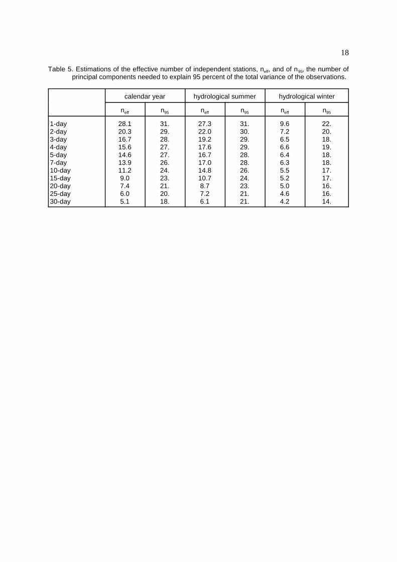
(Essenwanger, 1986; Jolliffe, 1990). This technic has been used in the preliminary study of thestationarity of the k-day extreme series (Gellens, 2000) for building independent series. The number ofranked eigenvalues of the covariance matrix required to account for 95 percent of the total variance canbe used as indicator of the number of independent components in the series. This index n which95integrates more information than n based on the mean of the correlation coefficients proposed byeffStedinger is also given in Table 5 and can be compared with n . The two indices are decreasing witheffk and are larger for summer than for winter. For small k values the two indices are fairly close for thesummer season and the calendar year. For 165 stations, the n index starts with values close to 30 foreffk=1 and for the calendar year and summer extremes. It drops quickly with growing k and reaches valuessmaller than 10 for k greater than 10 in summer and values smaller than 5 for k greater than 20 in winter.The n index is always greater than n and decreases slowly with growing k values. Hosking and Wallis95 eff(1988) have shown by means of Monte Carlo simulations that n overestimates the effect of theeffcorrelation on the estimation of the number of effective independent stations and it is thereforesuggested here to adopt n instead of n .95 eff

Obviously, the values of n are assessed by means of the 165 short-term stations and the95corresponding number of data is thus n* = n ×45. Considering the 9 long-term stations, this figure can95be put to n* = n ×45+n’ ×(86-45) to take into account the historical data, where n’ is the number of95 95 95principal components built with the historical series and needed to account for 95 percent of their totalvariance. This value probably underestimates the number of data but will not create artificially sharpconfidence intervals.

By the same reasoning, the value of m in the variance of the at-site mean can be assumed to be 86 inthe case of historical series but it has to be reduced for the short-term series. Sneyers (1975) introducedthe concept of equivalent size of series of which the parameters have been improved by means of areference long-term series. This figure m iseq

where m =45 is the length of the short-term data set, m =86 the length of the historical data set and �s l sltheir correlation. For example, m =51 for � =0.5 and m =59 for � =0.7.eq sl eq sl

According to these proposals to assess n* and m it is possible to estimate the confidence intervals ofthe growth curves and of the fractile curves. The upper and lower bounds, U and U , of theinf supconfidence interval corresponding to a � = 0.95 probability level are0

and (10)where N is the fractile of the reduced Normal distribution corresponding to the probability level �.�

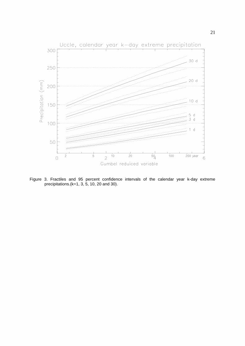
Replacing by and equating to 1 in expression (10) gives the confidence interval of thegrowth curve. Figure 3 shows the fractiles curves and their confidence intervals for the historical stationUccle for a selection of k values.

Discussion and conclusion

Usually data extension procedure and regionalisation are not combined. Usually in the regionalisation,long-term and short-term series are placed on the same level by normalizing (see expression 1) theircontribution with respect to their length. Long-term series have thus more weight than the short-termseries but they are not used as reference. In the present case the 9 historical series would have beencompletely hidden by the 165 stations of the climatological network.

The present study has shown the interest in climatology to use the data of a few well-documentedstations in a regional approach by giving them a central role, i.e. using them to improve the estimationof the at-site means and giving the opportunity to place some non stationary data sets in the stationaryframework of the long-term series. Of course this procedure requires a dense station network and is onlyfruitfully applicable when the mean correlation between the short-term and the reference long-termseries is higher than approximately 0.5. Some improvement of the procedure could be proposed in the

10

future. In particular it is clear that the number of historical stations can be enlarged and the addition ofone or two stations in the north of the country could be very useful to get a more regular density ofreference stations. Other conceptual improvements could also be introduced by modifying the dataextension procedure exploiting more, e.g. the correlation between the series. But in any case theefficiency of this modification ought to be compared with the method presented here.

The procedure presented here is certainly not as good as having all the data sets of all the stationsavailable in a well-documented data base. The encoding of the old data only available on paperdocuments is nevertheless requiring a careful preparation, a lot of time and devoted employees. It is inmany cases very difficult to find quickly the meta-data to identify the changes of location of the stationor the changes of instruments. The method proposed here allows thus to cope with the many commondifficulties in the data base management by according a particular attention to a restricted sample oflong-term stations. Although the present methodology has been applied here to the Belgian rainfallrecords, it is clear that it might be of interest for other climatological variables and certainly for othercountries.

Acknowledgements

The author wish to thank Dr D Koutsoyiannis and an anonymous reviewer for their constructive remarksand also Dr A. Buishand for his suggestions and support in this analysis.

References

Bultot, F. and Dupriez, G. L., 1976. Simulation of a series of daily areal mean rainfalls for a basin usingrainfall observations at a reference station located outside the catchment. Hydrol. SciencesBulletin, XXI/4, 569-585.

Buishand, T., A., 1991. Extreme rainfall estimation by combining data from several sites. Hydrol.Science Journal, 36, 345-365.

Buishand, T., A. and Demarée, G. R., 1990. Estimation of the annual maximum distribution fromsamples of maxima in separate seasons. Stochastic Hydrology and Hydraulics, 4, 89-103.

Cunnane, C., 1988. Methods and merits of regional flood frequency analysis. J. of Hydrology, 100: 269-290.

Cong, S., Li, Y., Vogel, J. L. and Schaake, J. C., 1993. Identification of the underlying distribution formof precipitation by using regional data. Water Resour. Res., 29: 1103-1111.

Delbeke, L., 2001. Extreme neerslag in Vlaanderen. Nieuwe IDF-curven gebaseerd op langdurigemeetreeksen van neerslag. Deel I. Volgens de methode van de jaarlijkse maxima..Ministerievan de Vlaamse Gemeenschap, afdeling water. 156 pp.

Demarée, G., 1985. Intensity-duration-frequency relationship of Point Precipitation at Uccle. Referenceperiod 1934-1983. Publication Série A, No 116, Inst. R. Météorol. Belg.

Dupriez, G., L. and Demarée, G., 1988. Contribution à l’étude des relations intensité-durée-fréquencedes précipitations. Totaux pluviométriques sur des périodes continues de 1 à 30 jours. I.Analyse de 11 séries pluviométriques de plus de 80 ans. Publication I.R.M., Miscellanea SérieA, No 8, 154 pp.

Dupriez, G., L. and Demarée, G., 1989. Contribution à l’étude des relations intensité-durée-fréquencedes précipitations. Totaux pluviométriques sur des périodes continues de 1 à 30 jours. Analysedes séries pluviométriques d’au moins 30 ans. Publication I.R.M., Miscellanea Série A, No 9,53 pp.

Essenwanger, O. M., 1986. Elements of Statistical Analysis. General Climatology, 1B, Ed. Landsberg,Elsevier, 424 pp.

Frich, P., Alexandersson, H., Aschcroft, J., Dahlström, B., Demarée, G. R., Drebs, A., van Engelen, A.F. V., Førland, E. J., Hanssen-Bauer, I., Heino, R., Jónsson, T., Jonasson, K., Keegan, L.,Nordli, P. Ø., Schmith, T., Steffensen, P., Tuomenvirta, H. and Tveito, O. E., 1996. North AtlanticClimatological Dataset (NACD Version 1) - Final Report. Danish Meteorological Institute.Scientific Report. 96-1, Copenhagen. 47 pp + annexes.

Gellens, D., 1995. Extreme precipitation of December 1993 and January 1995 in Belgium: ahomogenization procedure for the estimation of fractiles corresponding to long return periods.

11

Physics and Chemistry of the Earth, vol. 20, No 5-6, 451-454Gellens, D, 1998. The climate of the extreme values of the k-days precipitation amounts over Belgium.

Test of the homogenization by means of the fractile method. Proceedings of the 2 Europeand

Conference on Applied Climatology, 19-23 October 1998, Österreichische Beiträge zuMeteorologie und Geophysik, Nr. 19, Central Institute for Meteorology and Geophysiks, Vienna,Austria, 6pp.

Gellens, D., 2000. Trend analysis of k-day extreme precipitation over Belgium by means of non-parametric tests and principal components. Theor. Appl. Climatol., 66, 117-129.

Greenwood, J. A., Landwehr, J. M., Matalas, N. C. and Wallis J. R., 1979. Probability weightedmoments: definition and relation to parameters of several distributions expressable in inverseform. Water Resour. Res., 15, 1049-1054.

Hosking, J.R.M., 1997. FORTRAN routines for use with the method of L-moments, version 3.02, Res.Rep. RC20525, IBM Res. Div., Yorktown Heights, NY.33 pp.

Hosking, J. R. M. and Wallis, J. R., 1988. The effect of intersite dependence on regional flood frequencyanalysis. Water Resour. Res., 24, 588-600.

Hosking, J. R. M. and Wallis, J. R., 1993. Some statistics useful in regional frequency analysis. WaterResour. Res., 29, 271-281.

Hosking, J. R. M. and Wallis, J. R., 1997. Regional Frequency Analysis. An Approach based on L-Moments. Cambridge University Press, pp 224

Hosking, J. R. M., Wallis, J. R. and Wood, E. F., 1985. Estimation of the generalized extreme-valuedistribution by the method of the probability-weighted moments. Technometrics, 27, 251-261.

Jenkinson, A.F., 1969. Estimation of floods. WMO Technical Note N°98, (WMO - N°223), chapter 5, pp183-257. Geneva.

Jenkinson, A.F., 1977. The analysis of meteorological and other geophysical extremes. Met. O. 13.Branch Memorandom. No 58.

Jolliffe, I. T., 1990. Principal component analysis: a beginner’s guide - I. Introduction and application.Weather, 45, 375-382.

Landwehr, J. M., Matalas, N. C. and Wallis, J. R., 1979. Probability weighted moments with sometraditional techniques in estimating Gumbel parameters and quantiles. Water Resour. Res., 15,1055-1064.

Lu L.-H. and Stedinger, J. R., 1992a. Sampling variance of normalized GEV/PWM quantile estimatorsand a regional homogeneity test. J. Hydrol., 138, 223-245.

Lu L.-H. and Stedinger, J. R., 1992b. Variance of two- and three-parameter GEV/PWM quantileestimators: formulae, confidence intervals, and a comparison. J. Hydrol., 138, 247-267.

Rosbjerg, D. and Madsen, H., 1995. Uncertainty measures of regional flood frequency estimators. J.Hydrol., 167, 209-224.

Sneyers, R., 1961. On a special distribution of maximum values. Publication I.R.M., Contributions, No65, 4 pp.

Sneyers, R., 1975. Sur l’analyse statistique des séries d’observations. OMM Note Technique N°143,(OMM - N°415), 192 pp. Geneva.

Sneyers, R., 1977. L’intensité maximale des précipitations en Belgique. Publication I.R.M., Série B, No86, 15 pp.

Sneyers, R., 1979. L’intensité et la durée maximales des précipitations en Belgique. Publication I.R.M.,Série B, No 99, 19 pp.

Stedinger, J. R., 1983. Estimating a regional flood frequency distribution. Water Resour. Res., 19, 503-510.

Stedinger, J., Vogel, R. and Foufoula-Georgiou, E., 1993. Frequency analysis of extreme events. InHandbook of Hydrology. Ed. D. Maidment. Chapter 18, McGraw-Hill, New York, NY.

12

Figure captions

Figure 1. Location map of the climatological and historical stations.

Figure 2. Regional GEV parameters of the k-day extreme precipitation for the calendar year and thehydrological summer and winter.

Figure 3. Fractiles and 95 percent confidence intervals of the calendar year k-day extremeprecipitations.(k=1, 3, 5, 10, 20 and 30).

�hist

F200

13

Table captions

Table 1. Heterogeneity measures H and H applied on the k-day extreme value series of the calendar3year and of the hydrological summer and winter of the 9 historical (long-term) and of the 165short-term stations. Bold figures are higher than 1 and underlined are higher than 3.

Table 2. Average mean values of the summer and winter k-day extreme precipitation with k=1, 3, 10 and30. Residual mean square error (rms) of the means without (no est.) and with estimation of n=1,5,10, 20, 30, 40 and 50 randomly located missing values. The labels est. reg corresponds to theregional growth curve procedure, while est. Gumbet and est. GEV correspond respectively tothe procedures based on the Gumbel and on the GEV distributions. Bold figures indicate thesmaller rms value for each comparison. Mean correlation between the series with missingvalues and their reference complete station. Shadowed cells indicate the cases where the rmsof the means is smaller with the estimation of the missing values than without.

Table 3. Mean Jackknifed 200-year fractile values of the summer and winter k-day extremeprecipitation with k=1, 3, 10 and 30. Same residual mean square error as in table 2 for the 200-year fractiles.

Table 4. Mean correlation between short-term series and their corresponding reference historical series.Shadowed cells indicate the cases where the mean correlation is larger than the 0.52 threshold.

Table 5. Estimations of the effective number of independent stations, n , and of n , the number ofeff 95principal components needed to explain 95 percent of the total variance of the observations.

14

Table 1. Heterogeneity measures H and H applied on the k-day extreme value series of the calendar3year and of the hydrological summer and winter of the 9 historical (long-term) and of the 165short-term stations. Bold figures are higher than 1 and underlined are higher than 3.

long-term series short-term series

calendar year hydrological hydrological calendar year hydrological hydrologicalsummer winter summer winter

k H H H H H H H H H H H H3 3 3 3 3 3

1 -0.42 0.18 0.37 -0.26 0.88 0.01 -1.04 0.87 -0.25 0.52 -1.212 -1.09 -1.38 0.78 -0.95 0.05 -1.87 -1.81 0.41 -2.52 -3.49 -3.343 -0.78 -0.77 0.71 -0.77 0.37 -1.08 -2.61 -0.94 -4.73 -2.804 -0.44 0.05 0.77 -0.61 0.30 -0.63 -2.29 -4.17 -2.325 -0.17 0.54 -0.92 0.11 0.63 -0.41 -2.83 -3.217 -0.57 -0.73 -0.75 0.45 -0.83 -0.61 -1.70 -2.0110 -0.79 -0.92 -1.29 -0.33 -1.12 -1.73 -0.88 -1.5115 -1.73 -0.29 0.06 -0.80 -1.10 0.12 0.8220 -0.96 -0.37 0.41 0.12 -1.59 0.6125 0.12 -0.93 -0.08 0.24 -0.50 -1.8430 0.75 -1.43 -0.03 -0.13 0.03 -3.00

1.09 0.520.50 -1.26-0.38 -0.440.42 -0.90 1.70-0.05 -3.06 1.500.38 -3.54 -3.030.53 -4.40 -4.18

1.940.34-0.05 1.910.84 1.753.36

3.570.56 1.081.06 3.33-0.04 -1.82-2.64-4.19-5.45

3.25

2.26-1.91-3.17

1.77-2.04-5.23

�hist

�hist

15

Table 2. Average mean values of the summer and winter k-day extreme precipitation with k=1, 3, 10 and30. Residual mean square error (rms) of the means without (no est.) and with estimation of n=1,5,10, 20, 30, 40 and 50 randomly located missing values. The labels est. reg corresponds to theregional growth curve procedure, while est. Gumbet and est. GEV correspond respectively tothe procedures based on the Gumbel and on the GEV distributions. Bold figures indicate thesmaller rms value for each comparison. Mean correlation between the series with missingvalues and their reference complete station. Shadowed cells indicate the cases where the rmsof the means is smaller with the estimation of the missing values than without.

hydrological summer hydrological winter

m i s s i n g 1-day 3-day 10-day 30-day 1-day 3-day 10-day 30-dayvalue(s)

mean (mm) 34,754 50,135 83,27 150,622 30,128 51,863 92,324 165,52

1 no est. 0.2722 0.4513 0.1246 0.2020 0.2996 0.4989est. reg. 0.2760 0.1183 0.1754 0.3589

est. Gumbelest. GEV

0.1499 0.18200.1807 0.2037 0.3717 0.22280.1856 0.2040 0.2714 0.3759 0.1168 0.1715 0.2247 0.35050.1916 0.2083 0.2784 0.4059 0.1178 0.1751 0.2337 0.3492

5 no est. 0.6309 1.0340 0.2848 0.4724 0.7000 1.1704est. reg. 0.6302 0.2651 0.3974 0.8290

est. Gumbelest GEV

0.3476 0.42590.4263 0.4752 0.8388 0.50530.4401 0.4762 0.6203 0.8500 0.2615 0.3885 0.5101 0.81150.4568 0.4893 0.6374 0.9333 0.2652 0.3970 0.5383 0.8245

10 no est. 1.5162 0.4165 0.6871 1.0113 1.7131est. reg. 0.3935 0.5792 1.2145

est. Gumbelest. GEV

0.5033 0.6155 0.91150.6108 0.6867 0.9279 1.2465 0.74780.6301 0.6894 0.9126 1.2631 0.3882 0.5680 0.7543 1.18950.6597 0.7102 0.9348 1.3641 0.3938 0.5806 0.7949 1.2065

20 no est. 2.3327 0.6356 1.0391 1.5420 2.6013est. reg. 0.5968 0.8860 1.8402

est. Gumbelest. GEV

0.7642 0.9307 1.38040.9336 1.0425 1.4116 1.9129 1.13820.9693 1.0490 1.3904 1.9316 0.5889 0.8681 1.1488 1.79961.1468 1.1180 1.4195 2.0721 0.8272 0.8952 1.2258 1.8346

30 no est. 3.0598 0.8493 1.3870 2.0378 3.3936est. reg. 0.7874 1.1642 2.4178

est. Gumbelest. GEV

1.0169 1.2460 1.84731.2369 1.3825 1.8708 2.5463 1.49721.2934 1.3970 1.8489 2.5829 0.7804 1.1430 1.5164 2.37831.6747 1.5887 1.9275 2.7404 0.8573 1.1914 1.6475 2.4354

40 no est. 3.8279 1.0922 1.7673 2.5501 4.2747est. reg. 1.0246 1.5160 3.0963

est. Gumbelest. GEV

1.2954 1.5729 2.32341.5850 1.7850 2.3880 3.2261 1.91301.6557 1.8117 2.3609 3.2713 1.0212 1.4977 1.9468 3.05054.2341 3.1111 2.4656 3.4715 2.5929 1.6206 2.0533 3.1189

50 no est. 4.8194 1.3848 2.2098 3.2523 5.3728est. reg. 1.9393 3.8979

est. Gumbelest. GEV

1.6210 1.9867 2.93761.9612 2.2292 2.9941 4.1045 1.2922 2.44312.0449 2.2727 2.9764 4.1624 1.2961 1.9278 2.4994 3.85503.1255 2.7355 3.0927 4.5729 9.8495 2.3454 4.8893 4.0213

0,353 0,424 0,515 0,622 0,533 0,658 0,735 0,767

F200

F200

�hist

16

Table 3. Mean Jackknifed 200-year fractile values of the summer and winter k-day extremeprecipitation with k=1, 3, 10 and 30. Same residual mean square error as in table 2 for the 200-year fractiles.

hydrological summer hydrological winter

m i s s i n g 1-day 3-day 10-day 30-day 1-day 3-day 10-day 30-dayvalue(s)

(mm) 89,4 112,14 163,5 265,68 73,84 121,45 175,49 299,73

1 no est. 3.28 3.81est. reg. 3.73

est. Gumbel 3.68est. GEV

2.01 1.63 2.05 2.09 1.92 2.162.52 2.10 2.49 3.26 2.20 2.19 2.262.69 2.14 2.49 3.35 2.20 2.17 2.302.94 2.37 2.92 4.31 2.21 2.25 2.63 3.65

5 no est. 6.71 7.69est. reg. 7.42

est. Gumbelest. GEV

3.49 3.33 4.27 3.15 3.73 4.304.86 4.48 5.29 6.45 3.42 4.38 4.535.45 4.57 5.32 6.69 3.42 4.33 4.64 7.236.34 5.41 6.69 9.88 3.63 4.62 6.04 8.32

10 no est. 9.47 10.96est. reg. 10.62

est. Gumbelest. GEV

4.70 4.70 6.08 4.27 5.31 6.146.40 6.15 7.38 9.14 4.57 6.04 6.267.41 6.30 7.40 9.42 4.60 6.03 6.43 10.239.26 7.89 9.39 13.14 5.09 6.62 8.66 11.59

20 no est. 13.74 6.48 9.37 16.22est. reg. 15.72

est. Gumbelest. GEV

6.91 7.04 9.03 8.168.56 8.70 10.32 13.33 6.35 8.51 8.9110.47 8.97 10.48 13.46 6.54 8.65 9.20 14.7719.23 14.04 14.12 19.98 11.31 10.37 14.15 16.68

30 no est. 18.21 8.74 11.00 12.61 21.09est. reg. 20.54

est. Gumbelest. GEV

9.11 9.31 11.969.77 10.60 12.60 16.99 7.87 10.46 10.7812.68 11.17 12.93 17.06 8.29 10.79 11.27 19.2826.55 24.34 20.97 23.90 14.26 14.54 20.99 22.76

40 no est. 11.70 15.24 23.12 11.21 14.05 15.68 26.75est. reg. 24.99

est. Gumbelest. GEV

10.98 12.26 14.62 20.36 8.99 12.27 12.5315.09 13.23 15.26 20.45 9.81 13.15 13.45 23.7544.32 33.88 27.29 30.84 21.09 21.58 23.77 28.62

11.89

50 no est. 14.62 15.03 19.76 29.31 14.38 17.96 20.20 34.31est. reg. 29.59

est. Gumbelest. GEV

11.70 13.88 16.57 23.67 9.96 13.93 14.3817.12 15.62 18.14 24.11 11.42 15.56 15.95 28.6051.22 45.57 35.23 40.54 29.08 33.36 35.54 39.07

0.353 0.424 0.515 0.622 0.533 0.658 0.735 0.767

17

Table 4. Mean correlation between short-term series and their corresponding reference historical series.Shadowed cells indicate the cases where the mean correlation is larger than the 0.52 threshold.

1-day 2-day 3-day 4-day 5-day 7-day 10-day 15-day 20-day 25-day 30-day

c a l e n d a r 0.44 0.51 0.53 0.57 0.58 0.58 0.6 0.65 0.68 0.7 0.73year

hydrological 0.45 0.49 0.5 0.52 0.52 0.53 0.54 0.59 0.63 0.64 0.65summer.

hydrological 0.6 0.69 0.72 0.73 0.73 0.76 0.79 0.81 0.82 0.84 0.84winter

18

Table 5. Estimations of the effective number of independent stations, n , and of n , the number ofeff 95principal components needed to explain 95 percent of the total variance of the observations.

calendar year hydrological summer hydrological winter

n n n n n neff 95 eff 95 eff 95

1-day 28.1 31. 27.3 31. 9.6 22.2-day 20.3 29. 22.0 30. 7.2 20.3-day 16.7 28. 19.2 29. 6.5 18.4-day 15.6 27. 17.6 29. 6.6 19.5-day 14.6 27. 16.7 28. 6.4 18.7-day 13.9 26. 17.0 28. 6.3 18.10-day 11.2 24. 14.8 26. 5.5 17.15-day 9.0 23. 10.7 24. 5.2 17.20-day 7.4 21. 8.7 23. 5.0 16.25-day 6.0 20. 7.2 21. 4.6 16.30-day 5.1 18. 6.1 21. 4.2 14.

19

Figure 1. Location map of the climatological and historical stations.

regional GEV location parameter

0,825

0,85

0,875

0,9

0,925

1 10 100

k

loca

tion winter

summer

year

regional GEV scale parameter

0,175

0,2

0,225

0,25

0,275

1 10 100

k

scal

e summer

winter

year

regional GEV shape parameter

-0,1

-0,05

0

0,05

0,1

1 10 100

k

shap

e

wintersummer

year

20

Figure 2. Regional GEV parameters of the k-day extreme precipitation for the calendar year and thehydrological summer and winter.

21

Figure 3. Fractiles and 95 percent confidence intervals of the calendar year k-day extremeprecipitations.(k=1, 3, 5, 10, 20 and 30).