
Combining Machine Learning and Formal Methods for Complex ...
141
Universit ` a degli Studi di Udine Dipartimento di Scienze Matematiche, Informatiche e Fisiche Dottorato di Ricerca in Informatica e Scienze Matematiche e Fisiche Ph.D. Thesis Combining Machine Learning and Formal Methods for Complex Systems Design Candidate Simone Silvetti Supervisor Prof. Alberto Policriti Co-Supervisor Prof. Luca Bortolussi Tutor Dr. Enrico Rigoni Cycle XXX — A.Y. 2018
Transcript of Combining Machine Learning and Formal Methods for Complex ...

Universita degli Studi di Udine
Dipartimento di Scienze Matematiche,Informatiche e Fisiche
Dottorato di Ricerca in
Informatica e Scienze Matematiche e Fisiche
Ph.D. Thesis
Combining Machine Learning andFormal Methods for Complex
Systems Design
Candidate
Simone Silvetti
Supervisor
Prof. Alberto Policriti
Co-Supervisor
Prof. Luca Bortolussi
Tutor
Dr. Enrico Rigoni
Cycle XXX — A.Y. 2018

Institute ContactsDipartimento di Scienze Matematiche, Informatiche e FisicheUniversita degli Studi di UdineVia delle Scienze, 20633100 Udine — Italia+39 0432 558400http://www.dimi.uniud.it/
Author’s ContactsVia della raffineria, 734138 Trieste — Italiahttp://simonesilvetti.com

Ai miei nonni


Ringraziamenti
Nel corso di questi anni di dottorato ho potuto contare sulla disponibilita, il sostegno e iconsigli di diverse persone che con stima e affetto intendo ricordare in queste poche righe.
In primo luogo, devo molto di quanto appreso non solo alle favorevoli condizionidi lavoro e di ricerca all’interno dell’azienda Esteco, ma anche e in special modo, alcostante e proficuo dialogo con Luca Bortolussi, Alberto Policriti, Laura Nenzi ed EzioBartocci, che ringrazio per la disponibilita, le conversazioni stimolanti e la pazienza.
Un ringraziamento speciale – anche se ogni ringraziamento, seppur speciale, nonsara mai abbastanza – alla mia famiglia per aver sostenuto tutte le scelte che mi hannoportato fino a qui, e a Luisa, che con il suo affetto ha reso questo percorso piu piacevoledi quanto gia non fosse prima. Tutto questo e anche merito vostro.


Abstract
During the last 20 years, model-based design has become a standard practice in manyfields such as automotive, aerospace engineering, systems and synthetic biology. Thisapproach allows a considerable improvement of the final product quality and reduces theoverall prototyping costs. In these contexts, formal methods, such as temporal logics,and model checking approaches have been successfully applied. They allow a precisedescription and automatic verification of the prototype’s requirements.
In the recent past, the increasing market requests for performing and safer devicesshows an unstoppable growth which inevitably brings to the creation of more and morecomplicated devices. The rise of cyber-physical systems, which are on their way tobecome massively pervasive, brings the complexity level to the next step and openmany new challenges. First, the descriptive power of standard temporal logics is nomore sufficient to handle all kind of requirements the designers need (consider, forexample, non-functional requirements). Second, the standard model checking techniquesare unable to manage such a level of complexity (consider the well-known curse of statespace explosion). In this thesis, we leverage machine learning techniques, active learning,and optimization approaches to face the challenges mentioned above.
In particular, we define signal convolution logic, a novel temporal logic suited todescribe non-functional requirements. We also use evolutionary algorithms and signaltemporal logic to tackle a supervised classification problem and a system design prob-lem which involves multiple conflicting requirements (i.e., multi-objective optimizationproblems). Finally, we use an active learning approach, based on Gaussian processes, todeal with falsification problems in the automotive field and to solve a so-called thresholdsynthesis problem, discussing an epidemics case study.

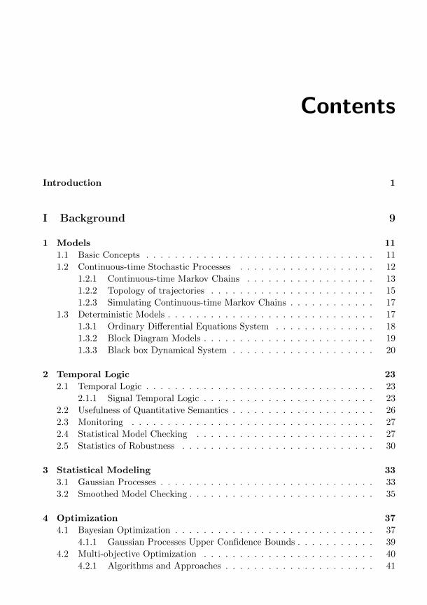
Contents
Introduction 1
I Background 9
1 Models 11
1.1 Basic Concepts . . . . . . . . . . . . . . . . . . . . . . . . . . . . . . . . 11
1.2 Continuous-time Stochastic Processes . . . . . . . . . . . . . . . . . . . 12
1.2.1 Continuous-time Markov Chains . . . . . . . . . . . . . . . . . . 13
1.2.2 Topology of trajectories . . . . . . . . . . . . . . . . . . . . . . . 15
1.2.3 Simulating Continuous-time Markov Chains . . . . . . . . . . . . 17
1.3 Deterministic Models . . . . . . . . . . . . . . . . . . . . . . . . . . . . . 17
1.3.1 Ordinary Differential Equations System . . . . . . . . . . . . . . 18
1.3.2 Block Diagram Models . . . . . . . . . . . . . . . . . . . . . . . . 19
1.3.3 Black box Dynamical System . . . . . . . . . . . . . . . . . . . . 20
2 Temporal Logic 23
2.1 Temporal Logic . . . . . . . . . . . . . . . . . . . . . . . . . . . . . . . . 23
2.1.1 Signal Temporal Logic . . . . . . . . . . . . . . . . . . . . . . . . 23
2.2 Usefulness of Quantitative Semantics . . . . . . . . . . . . . . . . . . . . 26
2.3 Monitoring . . . . . . . . . . . . . . . . . . . . . . . . . . . . . . . . . . 27
2.4 Statistical Model Checking . . . . . . . . . . . . . . . . . . . . . . . . . 27
2.5 Statistics of Robustness . . . . . . . . . . . . . . . . . . . . . . . . . . . 30
3 Statistical Modeling 33
3.1 Gaussian Processes . . . . . . . . . . . . . . . . . . . . . . . . . . . . . . 33
3.2 Smoothed Model Checking . . . . . . . . . . . . . . . . . . . . . . . . . . 35
4 Optimization 37
4.1 Bayesian Optimization . . . . . . . . . . . . . . . . . . . . . . . . . . . . 37
4.1.1 Gaussian Processes Upper Confidence Bounds . . . . . . . . . . . 39
4.2 Multi-objective Optimization . . . . . . . . . . . . . . . . . . . . . . . . 40
4.2.1 Algorithms and Approaches . . . . . . . . . . . . . . . . . . . . . 41

x Contents
II Contributions 45
5 Signal Convolution Logic 475.1 Signal Convolution Logic . . . . . . . . . . . . . . . . . . . . . . . . . . 49
5.1.1 Syntax and Semantics . . . . . . . . . . . . . . . . . . . . . . . . 515.1.2 Soundness and Correctness . . . . . . . . . . . . . . . . . . . . . 525.1.3 Expressiveness . . . . . . . . . . . . . . . . . . . . . . . . . . . . 54
5.2 Monitoring Algorithm . . . . . . . . . . . . . . . . . . . . . . . . . . . . 545.3 Case Study: Artificial Pancreas . . . . . . . . . . . . . . . . . . . . . . . 595.4 Conclusion and Future Works . . . . . . . . . . . . . . . . . . . . . . . . 63
6 Classification of Trajectories 676.1 Problem Formulation . . . . . . . . . . . . . . . . . . . . . . . . . . . . . 696.2 Methodology . . . . . . . . . . . . . . . . . . . . . . . . . . . . . . . . . 70
6.2.1 Discrimination Function . . . . . . . . . . . . . . . . . . . . . . . 716.2.2 GP-UCB: learning the parameters of the formula . . . . . . . . . 726.2.3 Genetic Algorithm: learning the structure of the formula . . . . 726.2.4 Regularization . . . . . . . . . . . . . . . . . . . . . . . . . . . . 74
6.3 Case Study: Maritime Surveillance . . . . . . . . . . . . . . . . . . . . . 746.4 Conclusion and Future Works . . . . . . . . . . . . . . . . . . . . . . . . 76
7 Parameter Synthesis 777.1 Problem Formulation . . . . . . . . . . . . . . . . . . . . . . . . . . . . . 797.2 Methodology . . . . . . . . . . . . . . . . . . . . . . . . . . . . . . . . . 80
7.2.1 Bayesian Parameter Synthesis: the Algorithm . . . . . . . . . . . 807.3 Case Studies . . . . . . . . . . . . . . . . . . . . . . . . . . . . . . . . . 837.4 Conclusion and Future Works . . . . . . . . . . . . . . . . . . . . . . . . 85
8 System Design with logical objectives 898.1 Problem Formulation and Methodology . . . . . . . . . . . . . . . . . . 908.2 Case Studies . . . . . . . . . . . . . . . . . . . . . . . . . . . . . . . . . 92
8.2.1 Genetic Toggle Switch . . . . . . . . . . . . . . . . . . . . . . . . 928.2.2 Epidemic model: SIRS . . . . . . . . . . . . . . . . . . . . . . . . 93
8.3 Results . . . . . . . . . . . . . . . . . . . . . . . . . . . . . . . . . . . . . 938.3.1 Genetic Toggle Switch . . . . . . . . . . . . . . . . . . . . . . . . 948.3.2 Epidemic model: SIRS . . . . . . . . . . . . . . . . . . . . . . . . 94
8.4 A deeper look at robustness . . . . . . . . . . . . . . . . . . . . . . . . . 968.5 Conclusion and Future Works . . . . . . . . . . . . . . . . . . . . . . . . 97
9 Falsification of Cyber-Physical Systems 999.1 Domain Estimation with Gaussian Processes . . . . . . . . . . . . . . . 1009.2 The Falsification Process . . . . . . . . . . . . . . . . . . . . . . . . . . . 101
9.2.1 Adaptive Optimization . . . . . . . . . . . . . . . . . . . . . . . . 1039.3 Probabilistic Approximation Semantics . . . . . . . . . . . . . . . . . . . 1059.4 Case Studies . . . . . . . . . . . . . . . . . . . . . . . . . . . . . . . . . 1079.5 Conclusion and Future Works . . . . . . . . . . . . . . . . . . . . . . . . 108

Contents xi
Concluding Remarks 111


List of Tables
4.1 Taxonomy of optimization problems . . . . . . . . . . . . . . . . . . . . 38
5.1 Signal Convolution Logic kernels . . . . . . . . . . . . . . . . . . . . . . 505.2 Performance of signal temporal logic vs signal convolution logic . . . . . 63
6.1 Results of the RObust GEnetic (ROGE) algorithm . . . . . . . . . . . . 75
7.1 Results of the statistical parameter synthesis approach to the SIR model 847.2 Scalability test of the statistical parameter synthesis approach . . . . . . 85
9.1 Results of the adaptive Probabilistic Approximation Semantics (PAS)approach to the falsification of the automatic transmission test case . . 107


List of Figures
1 Development Cycle Models . . . . . . . . . . . . . . . . . . . . . . . . . 1
1.1 Cyber-physical system plant . . . . . . . . . . . . . . . . . . . . . . . . . 121.2 A Cadlag function . . . . . . . . . . . . . . . . . . . . . . . . . . . . . . 161.3 A simple actor model . . . . . . . . . . . . . . . . . . . . . . . . . . . . . 201.4 Block diagram operators . . . . . . . . . . . . . . . . . . . . . . . . . . . 201.5 Block diagram models . . . . . . . . . . . . . . . . . . . . . . . . . . . . 21
4.1 Non-convex Pareto front (TNK problem) . . . . . . . . . . . . . . . . . 424.2 Genetic operators: mutation and crossover . . . . . . . . . . . . . . . . . 43
5.1 Graphical representation of signal convolution logic properties . . . . . . 485.2 Graphical representation of convolution and graphical intepretation of
signal convolution logic formulae . . . . . . . . . . . . . . . . . . . . . . 535.3 Sketch of signal convolution logic monitoring algorithm . . . . . . . . . 585.4 Signal temporal logic falsification vs signal convolution logic falsification 62
6.1 Anomalous and regular trajectories of the maritime surveillance test case 74
7.1 Partition of the parameter space . . . . . . . . . . . . . . . . . . . . . . 86
8.1 Comparison of the probability of satisfaction and robustness of signaltemporal logic formulae . . . . . . . . . . . . . . . . . . . . . . . . . . . 92
8.2 Comparison of the three optimization approaches for the SIRS test case 958.3 Comparison of the three optimization approaches for the genetic toggle
switch test case . . . . . . . . . . . . . . . . . . . . . . . . . . . . . . . 958.4 Pareto fronts of the maximization of the probability and average robust-
ness in the SIRS test case . . . . . . . . . . . . . . . . . . . . . . . . . . 968.5 Multi-objective approach to the robustness maximization of a signal tem-
poral logic formula . . . . . . . . . . . . . . . . . . . . . . . . . . . . . . 97
9.1 Example of probabilistic semantics and requirements of automatic trans-mission test case . . . . . . . . . . . . . . . . . . . . . . . . . . . . . . . 106


Introduction
Context
From past to present. During the last 20 years the market request of increasinglyperforming and safe devices shows an unstoppable growth. This trend is evident inmany fields, beginning with software and embedded device development, passing throughautomotive and aerospace fields and arriving at system and synthetic biology. The effectof this pressing demand had a big impact on all levels of industry organization startingfrom the internal organization and ending with the adoption of new system developmentmethodologies. In software engineering, for example, continuous delivery [HF10], test-driven development [Bec03] and agile approaches [Coc02] became de facto standardpractices. These approaches allow reducing the time-to-market of the released product,improving productivity, efficiency, and final product quality. Moreover, they ensure thepossibility to release software continuously over time, by fulfilling the demands of newfunctionality and following market’s direction.
The system development cycle rapidly changes to face the market requests, as well.It moves from a monolithic waterfall chain (Figure 1a) to a more flexible “V” model (Fig-ure 1b) which essentially replaces the previous chain with a new detailed and standardprocess.
(a) Waterfall Model(b) V model
Figure 1: Development Cycle Models
The requirement phase which is represented by the left side of the “V” starts with thedefinition and decomposition of the requirements and ends with the creation of system

2 Introduction
specifications. These specifications are then used to drive the implementation phasewhich is followed by the verification phase represented by the right side of the “V”.The novelty of this approach results in the possibility of concurrent execution of thethree steps described before, for example, the implementation and verification processescan start simultaneously, implying that the testing procedure is setting up before theimplementation. This strategy forces the implemented prototype to satisfy the originalrequirements from the beginning, which results in the minimization of the project’s riskand the improvement and assurance of quality of the final product.
Alongside the high-level vision which considers the product development cycle as aprocess to be optimized, there is a low-level vision which focuses on the three phasesforming this process: the requirements definition, the implementation, and the verifica-tion. All these three levels have been improved during the last 20 years.
In many fields, the implementation phase passed from the use of imperative languagesto object-oriented languages which more properly assist the development of complexand maintainable software. During 2000 many industries started to use the simulation-driven design processes, so that the Model-Based Development (MBD) quickly assumeda central role in system design. It aims to build computational models in place of realprototypes which can be simulated in order to verify their compliance with respect tooriginal requirements. Graphical Programming environments for modeling and simu-lation, such as Simulink [Mat] and LabVIEW [Nat], quickly become standard tools insuch fields as automatic control and signal processing [Cha17, TTS+08]. Their principalcontribution was the management, creation, and testing of complex in silico models byavoiding the standard implementation of code. The ability to create accurate modelsand executing them, rapidly increased and the MBD approach was adopted in many en-gineering industries (mainly automotive and aerospace). These new software programsand approaches bring new descriptive power at the designer’s disposal. As a conse-quence, the complexity of generated models increased and two outcomes arose. First,new challenges to the requirement definition and the verification phase were posed andsecondly the adoption of Multi-disciplinary Optimization (MDO) (i.e., the numericaloptimization approaches used to optimize specific model parameters) was granted.
A set of requirement specifications must adhere to the designer intention and mustbe coherent with the developing prototype. Too strict or not compatible requirementsgenerate errors during the testing and validation phase, and force the engineers tofix them, manage the implementations, and test/validate again the final prototype.All together, it results in increased time of the product development cycle. In somerestricted cases, formal methods have been adopted to overcome these situations. Theyact at the level of requirement definitions and consist in using formal languages, such astemporal logics and at the level of verification in using model checking techniques. Theuse of logical languages standardizes the definition of the requirements and reduces thepossibility of creating incompatible requirements. Model checking techniques give theopportunity of automatically verifying the satisfiability of these requirements, by freeingthe designer from the development of custom (and error-prone) verification algorithms.
Despite the undoubted usefulness of formal methods, which has been achieved anddemonstrated in specific high-level industrial fields, these methods are not yet used inmany other areas where they might be successfully applied. The reasons are rathercomplex. First of all there is a lack of knowledge in the field of formal methods (for
3
example many engineers do not even encounter them during their academic studies)and secondly there are many cases where standard model checking approaches are notdirectly applicable (e.g., they are not suitable to manage the complexity and size of themodel used in industries).
From present to future. Nowadays there is a growing interest in developing con-nected devices which assist our life. Starting from smart homes and continuing toself-driving vehicles, the presence of intelligent systems which autonomously interactwith humans and other devices is increasing. These systems are generally called Cyber-physical systems (CPS) [LS16], and their main feature is the integration of computationabilities within the physical world. These devices are able to collect and analyze datagenerated from physical sensors and to use this information to act and modify the phys-ical world around them, or at least spreading the information to other devices. Considera modern fly-by-wire aircraft. In this kind of airplane, the pilot’s commands are medi-ated by a computer control which, based on the actual aircraft conditions, could avoiderrors. It can prevent the aircraft to go outside the safe operating region and causing,for example, a stall. Cyber-physical systems are generally composed of multiple deviceswhich interact with each other and/or with the physical world even in a non-linear way.The main characteristics which make the CPS complex dynamical systems are theirnonlinearity and their hierarchical structure. The first implies that the understandingof the whole CPS cannot be derived by separately analyzing agents and combining thecollected information. The second characteristic means that, for example, the outputs ofsome devices are inputs of other devices. In some cases, circular dependencies can evenbe present, i.e., (closed) feedback loops. These two characteristics and the noisy natureof sensor data are the root causes of CPS complexity. The mathematical counterpart ofthis is the so-called state space explosion which makes the analysis of CPS a challengingtask of the present.
The forecast is clear: the use of CPS, which currently has an explosive growth, isgoing to be soon pervasive. Consider Industry 4.0, self-driving cars, medical devices,and smart grids. Every innovative technology field seems to engage CPS as the leadingactor of its storyboard. The improvement process necessary to master the complexity ofCPS touches all the level of MBD: requirements definition, implementation, verificationand also MDO. Moreover, considering the diffuse presence of CPS devices in our dailylife, their verification will assume a more and more central role.
This thesis can be collocated into the established path of research which tries tocombine formal methods and machine learning techniques for the verifiability and systemdesigns of complex systems.
Approach
Various mathematical models can be considered to describe CPS, and we can dividethem into two categories: Deterministic and Stochastic models. The former include Or-dinary Differential Equations or Finite State Machines which are widely used in popularmodeling software such as MATLAB/Simulink or LabVIEW. The latter include Contin-uous Time Markov Chain (CTMC) and Stochastic Hybrid Systems (SHS) mainly usedin population dynamics evolution such as biological reaction networks, epidemic mod-

4 Introduction
eling or performance evaluation. All these models can be simulated to produce possiblerealizations of the system, i.e., trajectories. These trajectories define the dynamics ofthe system induced by specific configurations (inputs and internal states). These modelscan be considered in the MBD framework which we introduced before. In this thesis,we focused on the above mentioned three aspects: requirements definition, verification,and optimization.
The first ingredient to properly define the requirements are formal languages such astemporal logic. These are modal logics suitable to describe in a rigorous and concise waytemporal behaviors. Among the existing temporal logics, we will focus our attentionon Signal Temporal Logic (STL), which is a linear, continuous-time, temporal logicwith future modalities, built on top of atomic predicates which are simple inequalitiesamong variables. The reason for this choice is twofold. First it is sufficiently powerful todescribe lots of phenomena, and secondly, it is easily interpretable. Moreover there existefficient monitoring algorithms which are capable of checking if a trajectory satisfies agiven STL formula or not.
The second ingredient is machine learning techniques aimed to assist the verificationof CPS. Given a requirement and a model, we could in principle use the standardmodel checking techniques to verify if the model is compliant with that requirement.If we consider stochastic models, for example, a requirement could be related to theprobability that a given temporal logic formula is satisfied. This is a standard task instochastic modeling, and several probabilistic model checkers have been implemented.Unfortunately, these model checkers are not able to work with complex systems suchas the majority of CPS. The mathematical counterpart is the well-known state spaceexplosion, which basically means that the state space of the systems increases so muchthat the exact model verification requires too much computational effort and memory.Statistical Model Checking (SMC) has been introduced to tackle this problem and try tosolve it in practice. The underlying idea is to approximate statistically the probability ofsatisfaction of a given formula by means of simulation. SMC effectively attacks the statespace explosion but can be applied only if the model is fully specified, meaning that,for example, all the chemical rates of a modeled chemical reactions have to be known.Obviously, this hypothesis is not reasonable in many situations. For example whensystem design and system identification problems are consisting precisely in determiningthose chemical rates! To overcome this situation smoothed model checking (smMC) hasbeen proposed. This technique relays on Gaussian processes, a regression techniquebelonging to Bayesian statistics, is the perfect example of combination of formal methodsand machine learning.
The third ingredient is the use of optimization techniques aiming at finding the bestperforming design with respect to a set of objectives. Mathematically this is tackled byseveral multi-objective optimization approaches primarily used in many industrial fields.These approaches regroup all the numerical algorithms which are able to simultaneouslyoptimize different objectives and to identify the so-called Pareto front (i.e., a set whichinformally represents the best compromise among different criteria/objectives).

5
Contribution
The leitmotif of this thesis is “master complexity of CPS”. The idea is to use novelmachine learning and optimization approaches to perform MBD of CPS in cases wherethe state of the art does not produce a good result.
As mentioned before, the requirement definition is a preliminary problem in MBD.We work on this subject acting in two opposite directions. In Chapter 6, we movefrom model/data to requirements by studying the problem of mining signal temporallogic formulae from a dataset composed of two kinds of trajectories (regular and anoma-lous). In machine learning, this task, known as classification problem, is a well-studiedproblem usually solved by means of dedicated algorithms. Efficient approaches, such asfeedforward neural networks, have been implemented even for big dataset. Such sys-tems produced black box computational models which are able to classify data withhigh accuracy, but paying a high price: low interpretability. It means that we cannotunderstand the reasons why a path is regular or anomalous. In a broader sense, wecannot extract knowledge from our dataset. Using Signal Temporal Logic (STL) is away to tackle such a problem, because it is a formalism sufficiently powerful to classifyobserved trajectories, and highly interpretable (thanks to its logical nature: an STLformula is a logical combination of simple linear inequalities). We use a genetic opti-mization algorithm which automatically combines STL formulae by leveraging on theirtree structure. In Chapter 5, we move from requirements to model/data by introducinga temporal logic called Signal Convolution Logic (SCL), a novel specification languagewhich can express non-functional requirements in cyber-physical systems showing noisyand irregular behavior. The STL language is not able to quantify about the percentageof time certain events happen. These kinds of requirements can be usefully considered inmodeling many CPS scenarios, e.g., medical devices. Consider, for instance, a medicalCPS device measuring glucose level in the blood to release insulin in diabetic patients.In this scenario, we need to check if glucose level is above (or below) a given thresholdfor a certain amount of time, to detect critical settings. Short periods of hyperglycemia(high level of glucose) are not dangerous for the patients. An unhealthy scenario iswhen the patient remains in hyperglycemia for more than 3 hours during the day, i.e.,for 12.5% of 24 hours. This property cannot be specified by STL.
The verification is another crucial step of MBD which is naturally linked to therequirement definition. We work on this subject by addressing synthesis and falsificationproblems which can be considered as two sides of the same coin. The first consistsin identifying the parameters which induce the model to behave as specified by therequirements. The second problem consists in identifying the parameters which causemalfunctions of the model. The faults are expressed through logical requirements. In[BPS16] we tackle the parameter synthesis problem in a multi-objective paradigm. Theidea consists in maximizing simultaneously the satisfaction probability of two (or more)logical formulae by obtaining a so-called Pareto front. The multi-objective approach tomodel checking verification has been already described in [EKVY07, CMH06, FKP12].The most common technique consists in transforming the original problem into a linearprogramming problem. Our approach is different. Similarly to the industrial approach,where the multi-objective paradigm is widely used, we consider the model as a blackbox and solve the multi-objective problem by customizing the dominance relation of astandard genetic algorithm (NSGAII, [DAPM02]). More specifically, we implemented a

6 Introduction
mixed approach consisting in maximizing the average robustness and the probability ofsatisfaction of two STL formulae. We show that this approach produces good resultsin two test cases. In Chapter 7, we deal with the parametrized verification of temporalproprieties which is an active research field of fundamental importance for the designof stochastic cyber-physical systems. In some domains (such as system and syntheticbiology) has become relevant to identify the region of the parameter space where themodel satisfies a linear time specification with probability greater (or less) than a giventhreshold. Solving this problem by employing numerical methods with guaranteed errorbounds has been considered in [CDKP14, CDP+17]. This method, however, is severelyaffected by the state space explosion problem. We proposed an alternative solution tothis problem employing machine learning and statistical approaches based on smoothedmodel checking. Moreover, we introduced the Bayesian threshold synthesis problem asthe statistical version of the threshold synthesis problem proposed in [CDP+17]. Theidea is to identify the region of the parameters space which induces a probability greater(or less) than a given threshold with statistical guarantees.
In [SPB17b] we implemented an active learning approach aimed at falsifying block-diagram models (i.e., Simulink/Stateflow, Scade, LabVIEW, etc.) where several switchblocks, 2/3-D look-up tables, and state transitions coexist. We cast the falsificationproblem into a domain estimation problem and used an active learning optimizationapproach, similar to the cross-entropy algorithm, which produces more and more coun-terexamples as the number of iterations increases. The inputs of these systems aremainly continuous, or cadlag functions, and for this reason a parametrization is manda-tory. We used an adaptive parametrization which is more expressive than the standardfixed point parametrization. Our approach is based on the active learning paradigmwhich consists in the simultaneous approximation and minimization of an unknownfunction (which in this case is the quantitative semantics of the STL requirements). Webring the approximation of the quantitative semantics at the logical level by defininga probabilistic approximation semantics. Briefly, we use the Gaussian processes to es-timate the probability that specific sub-formulae of the original STL requirement havebeen falsified. Then, this information is combined by means of a logical bottom-up ap-proach and the probability of falsifying the STL requirement is estimated. Afterward,this probability is used to sample points which eventually falsify the requirements. Thecombination of the active learning approach and the adaptive parametrization producesgood performance regarding the minimum number of simulations to falsify the model.This performance index is rather important in the industrial world where system simu-lations could be costly.
Thesis structure
This thesis has been divided into two parts. The first part presents the background whichis composed of 4 chapters. The second part outlines the contributions in 5 chapters.
Part I (Background). In Chapter 1, we introduce the basic definitions, the stochasticand deterministic models.
Chapter 2 describes the Signal Temporal Logic (STL) which is the main logic formal-ism used in the rest of the thesis. First, we introduce the Boolean and the quantitative

7
semantics, and then we summarize the model checking techniques focusing mainly onthe statistic model checking.
In Chapter 3, we describe Gaussian processes and how this nonparametric Bayesiantechnique can be efficiently employed to evaluate the probability of satisfaction of STLspecification of stochastic systems. This approach is known as smoothed model check-ing [BMS16].
In Chapter 4, we briefly introduce the mathematical techniques to solve optimizationproblems. We focus on Bayesian optimization and describe the evolutionary algorithmsable to solve the multi-objective optimization problems.
Part II (Contributions). In Chapter 5, we propose Signal Convolution Logic (SCL),a novel temporal logic suited to express non-functional requirements. This logic usesthe mathematical convolution to define a temporal operator which is able to quantifythe percentage of time an event occurs. This contribution has been accepted for pub-lication in the 16th International Symposium on Automated Technology for Verificationand Analysis (ATVA 2018). A preprint version of this contribution is available, see[SNBB18].
In Chapter 6, we use a genetic algorithm and the average robustness of STL formulasto create a classifier which can discriminate among anomalous and regular trajectories.This contribution has been accepted for publication in the 15th International Conferenceon Quantitative Evaluation of SysTems (QEST 2018). See [SNBB17] for a preprintversion of this work.
In Chapter 7, we combine the smoothed model checking technique with an activelearning approach to identify the parameter space of a parametrized model where thesatisfaction probability is above a given threshold. We rephrase this problem, known asthreshold synthesis problem, in a Bayesian framework and provide an algorithm whichefficiently solves it. This contribution has been published, see [BS18].
In Chapter 8, we study the design of stochastic systems in a multi-objective paradigm.The idea is to simultaneously maximize multiple conflicting requirements which are spec-ified employing STL formulae. This contribution has been published, see [BPS16].
Finally in Chapter 9, we present a new approach to tackle the falsification of formalproperties of a black box cyber-physical system. The proposed method leverages theGaussian processes and a new parameterization technique of the input functions toreduce the minimum number of simulation leading to the model falsification. Thiscontribution has been published, see [SPB17b].


IBackground


1Models
1.1 Basic Concepts
In this section we introduce the basic concepts which are the ground of the most of theresults in this thesis.
System. In a broader sense we intend a system as a collection of components. Weattach the adjective physical if these parts are physical objects or the adjectivelogical is these constituents are concepts such as algorithms or software.
State. The state of a system is the set of variables representing quantitative proprietiesof the system. Mathematically it is represented as a vector x = (x1, . . . , xn) ∈S, n ∈ N, expressing the quantitative values of the target properties.
Model. A model (of a system) is the description of specific aspects of the system. It hasa mathematical form which can be used to simulate the time evolution of specificquantities.
Trajectory (or signal). Informally it is the description of the time evolution of thesystem. Mathematically it is represented as the time evolution of its state vector,i.e., a function x : T → S, where the interval T ⊂ R+
0 represents the time and Sthe state space. We denote the trajectory space with ST.
Cyber-Physical Systems. CPS are systems composed by physical parts (mechanicalparts, chemical or biological processes), computational platforms (such as sensors,actuators, embedded devices), and network components which allow communica-tion among the computational platforms and different CPSs. The physical partsare essentially black box systems which react to the environment through physicalprocess. The computational parts are in charge of collecting information from thephysical parts by means of sensors and of elaborating this information in order totake actions.
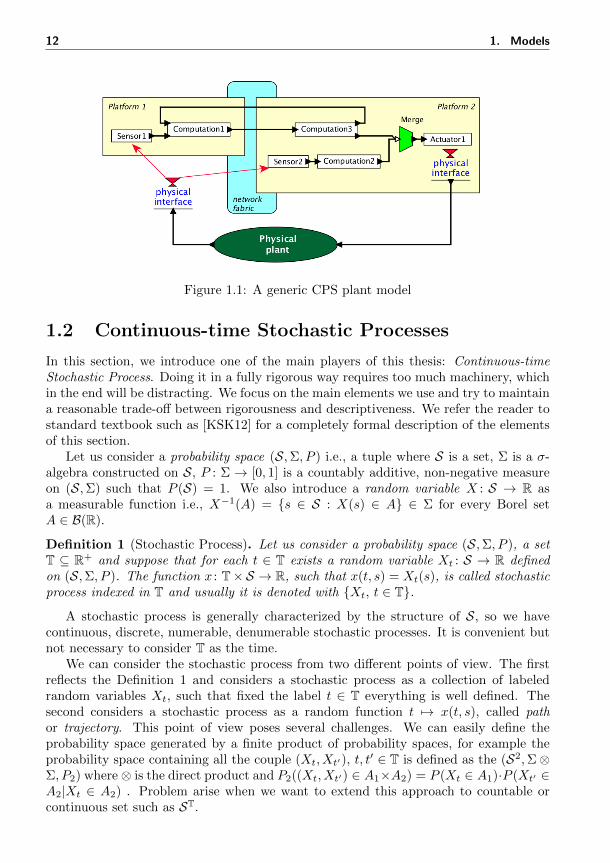
12 1. Models
Figure 1.1: A generic CPS plant model
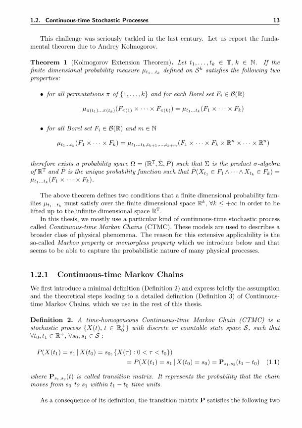
1.2 Continuous-time Stochastic Processes
In this section, we introduce one of the main players of this thesis: Continuous-timeStochastic Process. Doing it in a fully rigorous way requires too much machinery, whichin the end will be distracting. We focus on the main elements we use and try to maintaina reasonable trade-off between rigorousness and descriptiveness. We refer the reader tostandard textbook such as [KSK12] for a completely formal description of the elementsof this section.
Let us consider a probability space (S,Σ, P ) i.e., a tuple where S is a set, Σ is a σ-algebra constructed on S, P : Σ → [0, 1] is a countably additive, non-negative measureon (S,Σ) such that P (S) = 1. We also introduce a random variable X : S → R asa measurable function i.e., X−1(A) = s ∈ S : X(s) ∈ A ∈ Σ for every Borel setA ∈ B(R).
Definition 1 (Stochastic Process). Let us consider a probability space (S,Σ, P ), a setT ⊆ R+ and suppose that for each t ∈ T exists a random variable Xt : S → R definedon (S,Σ, P ). The function x : T×S → R, such that x(t, s) = Xt(s), is called stochasticprocess indexed in T and usually it is denoted with Xt, t ∈ T.
A stochastic process is generally characterized by the structure of S, so we havecontinuous, discrete, numerable, denumerable stochastic processes. It is convenient butnot necessary to consider T as the time.
We can consider the stochastic process from two different points of view. The firstreflects the Definition 1 and considers a stochastic process as a collection of labeledrandom variables Xt, such that fixed the label t ∈ T everything is well defined. Thesecond considers a stochastic process as a random function t 7→ x(t, s), called pathor trajectory. This point of view poses several challenges. We can easily define theprobability space generated by a finite product of probability spaces, for example theprobability space containing all the couple (Xt, Xt′), t, t
′ ∈ T is defined as the (S2,Σ⊗Σ, P2) where ⊗ is the direct product and P2((Xt, Xt′) ∈ A1×A2) = P (Xt ∈ A1)·P (Xt′ ∈A2|Xt ∈ A2) . Problem arise when we want to extend this approach to countable orcontinuous set such as ST.
1.2. Continuous-time Stochastic Processes 13
This challenge was seriously tackled in the last century. Let us report the funda-mental theorem due to Andrey Kolmogorov.
Theorem 1 (Kolmogorov Extension Theorem). Let t1, . . . , tk ∈ T, k ∈ N. If thefinite dimensional probability measure µt1...tk defined on Sk satisfies the following twoproperties:
• for all permutations π of 1, . . . , k and for each Borel set Fi ∈ B(R)
µπ(t1)...π(tk)(Fπ(1) × · · · × Fπ(k)) = µt1...tk(F1 × · · · × Fk)
• for all Borel set Fi ∈ B(R) and m ∈ N
µt1...tk(F1 × · · · × Fk) = µt1...tk,tk+1,...,tk+m(F1 × · · · × Fk × Rn × · · · × Rn)
therefore exists a probability space Ω = (RT, Σ, P ) such that Σ is the product σ-algebraof RT and P is the unique probability function such that P (Xt1 ∈ F1∧ · · ·∧Xtk ∈ Fk) =µt1...tk(F1 × · · · × Fk).
The above theorem defines two conditions that a finite dimensional probability fam-ilies µt1...tk must satisfy over the finite dimensional space Rk, ∀k ≤ +∞ in order to belifted up to the infinite dimensional space RT.
In this thesis, we mostly use a particular kind of continuous-time stochastic processcalled Continuous-time Markov Chains (CTMC). These models are used to describes abroader class of physical phenomena. The reason for this extensive applicability is theso-called Markov property or memoryless property which we introduce below and thatseems to be able to capture the probabilistic nature of many physical processes.
1.2.1 Continuous-time Markov Chains
We first introduce a minimal definition (Definition 2) and express briefly the assumptionand the theoretical steps leading to a detailed definition (Definition 3) of Continuous-time Markov Chains, which we use in the rest of this thesis.
Definition 2. A time-homogeneous Continuous-time Markov Chain (CTMC) is astochastic process X(t), t ∈ R+
0 with discrete or countable state space S, such that∀t0, t1 ∈ R+, ∀s0, s1 ∈ S :
P (X(t1) = s1 |X(t0) = s0, X(τ) : 0 < τ < t0)= P (X(t1) = s1 |X(t0) = s0) = Ps1,s2(t1 − t0) (1.1)
where Ps1,s2(t) is called transition matrix. It represents the probability that the chainmoves from s0 to s1 within t1 − t0 time units.
As a consequence of its definition, the transition matrix P satisfies the following two

14 1. Models
properties:
∀t ∈ R+, ∀s, s ∈ S, 0 ≤ Ps,s(t) ≤ 1 (1.2)
∀t ∈ R+, ∀s ∈ S,∑s∈S
Ps,s(t) = 1 (1.3)
Property 1.2 is a consequence of the definition of probability, and Property 1.3 saysmerely that the chain keeps its state or jumps to another state.
Equation 1.1 (up to the first equality sign) is called Markov property (also knownas memoryless property). It states that the conditional probability distribution of thefuture chain evolution depends only on the present state. Moreover, we are also statingthat the chain’s dynamics does not depend on the arrival times (t0) but only on thesojourn time (t1 − t0). This is the time homogeneity assumption. The Markovianproperty entails the semi-group property P(s + t) = P(s) ·P(t), also called Chapman-Kolmogorov Equations, which brings directly to the well known backward and forwardKolmogorov equations.
Assuming that P(t) is right-continuous and considering1 that P(0) = I, we definethe infinitesimal generator of a CTMC as
Q = limh→0+
P(h)− I
h(1.4)
Considering Properties 1.2 and 1.3, we have that∑s′∈S
Qs,s′ = 0 ; Qs,s ≤ 0 ; ∀s 6= s′, Qs,s′ ≥ 0 .
When s 6= s′ the value Qs,s′ is interpreted as the rate of moving for s to s′ and Qs,s =∑s′ 6=s Qs,s′ as the rate of leaving s.
Finally, considering Equation 1.4 and dP(t)dt = limh→0+
P(t+h)−P(t)h we obtain the
famous backword and forward Kolmogorov equations
dP(t)
dt= QP(t),
dP(t)
dt= P(t)Q
The solution is P(t) = etQ where the exponential of a matrix A is defined as eA =∑k∈N
Ak
k! .
Definition 3. A Continuous-time Markov Chain is a pair (S,R) where S is a finite(or countable) set of states and R is the rate matrix such that the dynamics is definedby
Ps,s′(t) =Rs,s′
E(s)
(1− e−E(s)t
), such that E(s) =
∑s′∈S
R(s, s′) (1.5)
The characterization of the transition matrix obtained in Equation 1.5 hints thatthe CTMCs are separable with respect to time and state transition. The first factor
1The semi-group property states that P(0)2 = P(0) which entails that P(0) is the identity matrixI.

1.2. Continuous-time Stochastic Processes 15
R(s, s′)/E(s) describes the jumping probability from s to s′ which is unaffected by thesojourn time t. Whereas the factor 1−e−E(s)t, which rules the time t within a future out-going transition happens, is fully agnostic to the ongoing destination s′. This separationis at the basis of many algorithms which simulate CTMC, and it is the reason why thesemodels are usually covered under the umbrella of jumping and holding stochastic process.
Throughout this thesis we mainly consider parametric reaction networks. We stressthat our approaches can be applied to every population models based on CTMCs, such asPopulation Continuous-time Markov Chains [BHLM13a] or Markov Population Models[HJW11].
Definition 4. A Parametric Reaction Network2 (PRN) is a tuple Mϑ =(A,S,x0,R, ϑ), where:
• A = a1, . . . , an is the set of species (or agents).
• x = (x1, . . . , xn) is the vector of variables counting the amount of each species,with values x ∈ S, where S ⊆ Nn is the state space.
• x0 ∈ S is the initial state.
• R = r1, . . . , rm is the set of reactions, each of the form rj = (vj, αj), with vj thestoichiometry or update vector and αj = αj(x, ϑ) the propensity or rate function.Each reaction can be represented as
rj : uj,1a1 + . . .+ uj,nanαj−→ wj,1a1 + . . .+ wj,nan,
where uj,i (wj,i) is the amount of elements of species ai consumed (produced) byreaction rj. We let uj = (uj,1, . . . , uj,n) (and similarly wj) and define vj = wj−uj.
• ϑ = (ϑ1, . . . , ϑk) is the vector of parameters, taking values in a compact hyperrect-angle Θ ⊂ Rk.
A PRNMϑ defines a Continuous-time Markov Chain [Nor98, BHLM13a] on S, withinfinitesimal generator Q, where Qx,y =
∑rj∈Rαj(x, ϑ) | y = x + vj, x 6= y.
1.2.2 Topology of trajectories
A useful definition, in the context of stochastic processes, is the following.
Definition 5 (Cadlag function). A Cadlag3 function X : T → S is a right continuousfunction with left-hand limit
(i) X(t) = limt→t+ X(t)
(ii) ∀t ∈ T, ∃ limt→t− X(t)
Thanks to their ability to describe jumps (which is a standard feature of stochas-tic trajectories), cadlag functions are largely used in the field of stochastic modeling.
2Also known as Parametric Chemical Reaction Network (PCRN).3French: “continue a droite, limite a gauche”.

16 1. Models
Figure 1.2: A Cadlag function
In this domain the uniform topology L∞(T,R), induced by the distance d∞(X,Y ) =supt∈[0,T ] ‖X(t)− Y (t)‖∞, is not satisfactory4. Let us consider a stochastic trace mod-eled by the Heaviside function H:
H : R→ 0, 1
H(t) =
0 t < 0
1 otherwhise
It describes a single jump from state x = 0 to x = 1 at time 0. If we consideranother trace H(t) := H(t−ε) which represents the same jump in almost the same timet = ε, ε 1, we would like to have guarantees that these two trajectories are close. Thisrequirement is natural if we consider that those two trajectories visit the same sequenceof locations at almost the same time. Unfortunately the uniform topology is unable tocapture that behavior, as implied indeed by ∀ε > 0 ‖H(x)−H(x+ ε)‖∞ = 1 > 0.
A practical example which evidences the lackingness of the uniform distance d∞comes out from the runtime verification area. During monitoring of trajectories couldhappen that small delays affect the measurement procedure. For this reason, it isnecessary to consider a measure which is not too much sensitive to such artifacts. TheSkorohod topology was introduced to solve this task.
Definition 6. (Skorohod Distance) Let Λ = TT be the set of the strictly increasingfunctions from T to T, and consider two cadlag functions X,Y : T→ R. The Skorohoddistance is
dsk(X,Y ) = infλ∈Λ
max(‖λ− 11‖∞, d∞(X,Y λ))
where 11 is the identity function, i.e., 11(x) := x.
This distance considers simultaneously the d∞ distance (between X and a deforma-tion of Y , i.e., Y λ) and a penalizing term which is proportional to the deformationinduced by λ ∈ Λ, i.e., ‖λ− 11‖∞. As a consequence of its strictly increasing trend, theλ functions preserve the original sequence of events, allowing, however, dilatations or
4If x = (x1, . . . , xn) then ‖x‖∞ = maxi≤n |xi|.
1.3. Deterministic Models 17
contractions of time. Informally, the Skorohod distance permits to manage perturba-tion of both space and time. We always work with trace defined on a closed subintervalT ⊂ R+
0 where the Skorohod distance is well defined. In other cases could be necessaryto extend its definition to the whole R+
0 . For a detailed explanation see [Bil99].
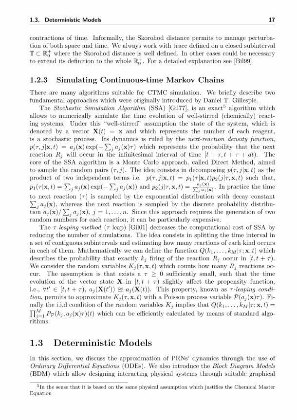
1.2.3 Simulating Continuous-time Markov Chains
There are many algorithms suitable for CTMC simulation. We briefly describe twofundamental approaches which were originally introduced by Daniel T. Gillespie.
The Stochastic Simulation Algorithm (SSA) [Gil77], is an exact5 algorithm whichallows to numerically simulate the time evolution of well-stirred (chemically) react-ing systems. Under this “well-stirred” assumption the state of the system, which isdenoted by a vector X(t) = x and which represents the number of each reagent,is a stochastic process. Its dynamics is ruled by the next-reaction density function,p(τ, j|x, t) = aj(x) exp(−
∑j aj(x)τ) which represents the probability that the next
reaction Rj will occur in the infinitesimal interval of time [t + τ, t + τ + dt). Thecore of the SSA algorithm is a Monte Carlo approach, called Direct Method, aimedto sample the random pairs (τ, j). The idea consists in decomposing p(τ, j|x, t) as theproduct of two independent terms i.e. p(τ, j|x, t) = p1(τ |x, t)p2(j|τ,x, t) such that,
p1(τ |x, t) =∑j aj(x) exp(−
∑j aj(x)) and p2(j|τ,x, t) =
aj(x)∑j aj(x) . In practice the time
to next reaction (τ) is sampled by the exponential distribution with decay constant∑j aj(x), whereas the next reaction is sampled by the discrete probability distribu-
tion aj(x)/∑j aj(x), j = 1, . . . , n. Since this approach requires the generation of two
random numbers for each reaction, it can be particularly expensive.The τ -leaping method (τ -leap) [Gil01] decreases the computational cost of SSA by
reducing the number of simulations. The idea consists in splitting the time interval ina set of contiguous subintervals and estimating how many reactions of each kind occursin each of them. Mathematically we can define the function Q(k1, . . . , kM |τ ; x, t) whichdescribes the probability that exactly kj firing of the reaction Rj occur in [t, t + τ).We consider the random variables Kj(τ,x, t) which counts how many Rj reactions oc-cur. The assumption is that exists a τ ≥ 0 sufficiently small, such that the timeevolution of the vector state X in [t, t + τ) slightly affect the propensity function,i.e., ∀t′ ∈ [t, t + τ), aj(X(t′)) u aj(X(t)). This property, known as τ -leaping condi-tion, permits to approximate Kj(τ,x, t) with a Poisson process variable P(aj(x)τ). Fi-nally the i.i.d condition of the random variables Kj implies that Q(k1, . . . , kM |τ ; x, t) =∏Mj=1 PP(kj , aj(x)τ)(t) which can be efficiently calculated by means of standard algo-
rithms.
1.3 Deterministic Models
In this section, we discuss the approximation of PRNs’ dynamics through the use ofOrdinary Differential Equations (ODEs). We also introduce the Block Diagram Models(BDM) which allow designing interacting physical systems through suitable graphical
5In the sense that it is based on the same physical assumption which justifies the Chemical MasterEquation

18 1. Models
workflows. These models are essentially hybrid systems with several internal stateswhich are associated with specific continuous dynamics described through ODEs sys-tems. The activation of these internal states, which is ruled by a specific guard mecha-nism, allows the modeling of complex dynamics, which are frequent in the field of CPS.Finally, we introduce the nonautonomous dynamical systems which are practically usedto model BDMs in the context of black box modeling.
1.3.1 Ordinary Differential Equations System
Let us consider the following reaction network with a1, . . . , an species and r1, . . . , rjreactions
r1 : u1,1a1 + . . .+ u1,nanα1−→ w1,1a1 + . . .+ w1,nan
r2 : u2,1a1 + . . .+ u2,nanα2−→ w2,1a1 + . . .+ w2,nan
. . . −→ . . .
rj : uj,1a1 + . . .+ uj,nanαj−→ wj,1a1 + . . .+ wj,nan
This reaction network can be modeled with an ODEs system as follows
dx1
dt=f1(x1, . . . , xj)
dx2
dt=f2(x1, . . . , xj)
. . . . . .
dxjdt
=fj(x1, . . . , xj)
where x1(t), . . . , xn(t) represent the percentage6 of the specie a1, . . . , an which populatethe reaction networks at time t and the functions f1, . . . , fj depend on the structureand the rates of the reaction. This approach was criticized by Daniel T. Gillespie in theintroduction of SSA original paper [Gil77]. Its primary concern is referred to the over-simplification of the non-deterministic and discrete nature of PRN to a continuous anddeterministic process. This approximation, which is reliable if the number of moleculesis sufficiently high, results from the following statement
∀i ≤ j, limn→+∞
∑nX
ni (0)
n= x(0) =⇒ ∀i ≤ j, lim
n→+∞P
sups≤t
∣∣∣∣∑nXni (s)
n− x(s)
∣∣∣∣ ≥ ε
= 0
which asserts that the averages of stochastic variables Xi evolve by following a de-terministic process ruled by the above ODEs. A formal proof of this statement can befound in [Kur70] and a detailed presentation of this topic, known as fluid approximation,is discussed in [BHLM13a].
Let us introduce an example to whom we refer a lot in the contribution part of thisthesis.
6It is a continuous approximation of the real percentage which assumes value in a discrete set.

1.3. Deterministic Models 19
Example 1. We consider a SIRS epidemic model, introduced back in 1927 by W.O.Kermack and A.G. McKendrick [GCC00], which is still widely used to simulate thespreading of a disease among a population. The population of N individuals is typicallydivided into three classes:
susceptible (S) : representing healthy individuals that are vulnerable to the infection.
infected (I) : describing individuals that have been infected by the disease and areactively spreading it.
recovered (R) : modeling individuals that are immune to the disease, by having recov-ered from the disease (R).
The chemical reactions are the following
r1 : S + Iα1−→ 2I α1 = ksi ·
Xs ·Xi
N
r2 : Iα2−→ R α2 = kir ·Xi
The corresponding ODE System is the following:
ds(t)
dt=− ksis(t)i(t)
di(t)
dt=ksis(t)i(t)− kiri(t)
dr(t)
dt=kiri(t)
(1.6)
1.3.2 Block Diagram Models
Many physical systems can be described employing multiple interacting ODEs systems.From a modeling point of view, it is convenient to have a tool which permits to graph-ically design and simulate such systems. Simulink [Mat], Modelica [Mod] and Lab-VIEW [Nat] are the most used software of this kind. These models, known as BlockDiagram Models (BDM), are based on the fundamental concept of Actor Model [HBS73]originated in 1973. An actor is a computational entity which receives messages fromother actors, use this information to change its internal state, and eventually producesoutputs which are spread to other connected actors. These models can be used to de-scribe a continuous-time system S which operates on continuous signals. The idea is todraw it as a graphical box with inputs and outputs as following
Mathematically S is a functional that depends on two parameters p and q
S(q, p) : RR → RR (1.7)
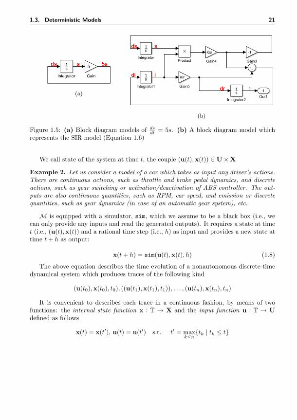
Multiple actor models can be collected and considered together as a unique entity, whichis considered again as a single actor model. This is the purpose of the subsystems blockwhich is shown in Figure 1.4, where also other common blocks are reported. Thisgrouping property allows hierarchically treating BDMs, enhancing the possibility tomanage different levels of complexity. In Figure 1.5a a block diagram model of an

20 1. Models
Figure 1.3: An actor model S which has an input (In1), an output (Out1) and dependson two parameters p and q.
ODE is represented. It consists of a simple feed-forward loop with an integrator anda gain block. Whereas, in Figure 1.5b we represent the SIR model (Example 1) as acombination of two feed-forward loops.
Figure 1.4: The most common operators are shown. We have the constant block whichsimply produces a constant output function, the gain block which multiplies by a factorthe input function. Then we see the integrator, sum and product blocks. The Subsystemblock
1.3.3 Black box Dynamical System
In the Introduction, we outlined the black box approach to modeling. It is a mandatoryapproach in the absence of a model’s internal specifications and a reasonable one ifthese specifications are too complicated. These two cases are a standard set up in manyindustrial fields, which indeed use this kind of approach. The idea is to model a systemas a pair M = (U×X , sim) where U and X are finite sets representing, respectively,the input values of the system and the internal state (coinciding for us with the output).The input set is characterized as follows:
U = U0 × · · · × Un × U1 × · · · × Um (input set)
where Ui are finite (or numerable) sets and Ui are compact sets in R, represent-ing respectively the discrete input events and the continuous input signals. A similarcharacterization is valid for the internal state
X = X0 × · · · × Xn′ ×X1 × · · · ×Xm′ (internal state set)
1.3. Deterministic Models 21
(a)
(b)
Figure 1.5: (a) Block diagram models of dsdt = 5s. (b) A block diagram model which
represents the SIR model (Equation 1.6)
We call state of the system at time t, the couple (u(t),x(t)) ∈ U×X
Example 2. Let us consider a model of a car which takes as input any driver’s actions.There are continuous actions, such as throttle and brake pedal dynamics, and discreteactions, such as gear switching or activation/deactivation of ABS controller. The out-puts are also continuous quantities, such as RPM, car speed, and emission or discretequantities, such as gear dynamics (in case of an automatic gear system), etc.
M is equipped with a simulator, sim, which we assume to be a black box (i.e., wecan only provide any inputs and read the generated outputs). It requires a state at timet (i.e., (u(t),x(t)) and a rational time step (i.e., h) as input and provides a new state attime t+ h as output:
x(t+ h) = sim(u(t),x(t), h) (1.8)
The above equation describes the time evolution of a nonautonomous discrete-timedynamical system which produces traces of the following kind
(u(t0),x(t0), t0), ((u(t1),x(t1), t1)), . . . , (u(tn),x(tn), tn)
It is convenient to describes each trace in a continuous fashion, by means of twofunctions: the internal state function x : T → X and the input function u : T → Udefined as follows
x(t) = x(t′), u(t) = u(t′) s.t. t′ = maxk≤ntk | tk ≤ t


2Temporal Logic
In the first part of this chapter, we introduce the temporal logics, mainly focusing onSignal Temporal Logic (STL), largely used to reason about the future evolution of apath in continuous time. In the second part, we describe the monitoring and the modelchecking techniques available.
2.1 Temporal Logic
Temporal logic [Pnu77] is a formalism tailored to reason about events in time. It extendsthe propositional or predictive logic by modalities (temporal operators) that permit tomanage time. These modalities are built on the couple (T, <), where T is the usual timeinterval and < is the accessibility relation on T. These formalisms permit a rigorousdescription of events in time, therefore are used to define temporal proprieties of dynam-ical systems. There are different kinds of temporal logics which are based on differentassumptions about the nature of time. It can be linear, if there is only a single timeline,or branched, if there exist multiple timelines (i.e., branches which can be representedas a tree). Moreover, we can consider time as a discrete, numerable or continuous set.We are mainly interested in a linear continuous-time temporal logic. Linear, becausewe deal with simulation trajectories and continuous-time because the systems, that wedescribe, have continuous dynamics.
2.1.1 Signal Temporal Logic
STL [MN04] has been introduced in 2004 with the purpose of defining properties ofcontinuous-time real-valued signals which can also be useful for the runtime verificationof dynamical systems’ trajectories. In that period many discussions were related to theverification of continuous hybrid systems and how the exhaustive and precise verificationof these systems was not decidable (except for trivial cases). STL extends MITL[a,b], afragment of the Metric Interval Temporal Logic (MITL) [AFH96] which uses boundedtemporal operators. Basically, STL redefines the atomic predicates of MITL into atomicpropositions interpreted over real-values signals.

24 2. Temporal Logic
We call primary signal a trajectory as defined in Section 1.1, it merely describesthe quantitative evolution of the state vector. We now recall the definition of Booleansignals, which are abstraction of primary signals, introduced to represent the qualitativetime evolution of specific properties. Finally, we present the syntax and semantics ofSTL.
Definition 7. Let us consider a primary signal x : T → S and the set of atomic pred-icates Π = f(s) ≥ 0 | f ∈ C(Rm,R), s ∈ S where C(Rm,R) is the set of continuousfunction from Rm to R. We call Boolean signal the function γ : T→ B = ⊥,> definedas γ(t) = π(x(t)) = (f x)(t) > 0. Moreover, we call secondary signal the functionf x : T→ R.
The secondary signal represents a quantity that we would like to monitor. It isa natural concept by a modeling and monitoring point of view and can be computedwith physical filters (i.e., specific devices which monitor trajectories), or computationalalgorithms usually called monitors.
Definition 8 (Syntax). The formulae of STL (denoted with LSTL) are defined by thefollowing syntax:
ϕ := ⊥ |> |µ | ¬ϕ |ϕ ∨ ϕ |ϕU[T1,T2]ϕ, (2.1)
where ⊥ and > denote logical false and true, ¬ and ∨ are the usual logical connectives,the atomic predicates µ ∈ Π have been defined before, [T1, T2] ⊂ R+
0 and U[T1,T2] isa temporal operator called Until. For simplicity, two other temporal operators Finallyand Globally can be defined as customary as F[T1,T2]ϕ ≡ >U[T1,T2]ϕ and G[T1,T2]ϕ ≡¬F[T1,T2]¬ϕ, respectively.
The formulae of LSTL are interpreted over trajectories respect to the followingBoolean semantics [MN04].
Definition 9 (Boolean Semantics). Given a trajectory x ∈ ST, the Boolean semantics|=⊂ (ST × R+
0 )× LSTL is defined recursively by:
(x, t) |= µ ⇐⇒ µ(x(t)) = >(x, t) |= ¬ϕ ⇐⇒ (x, t) 6|= ϕ
(x, t) |= ϕ1 ∨ ϕ2 ⇐⇒ (x, t) |= ϕ1 or (x, t) |= ϕ2
(x, t) |= ϕ1U[T1,T2]ϕ2 ⇐⇒ exists t′ ∈ [t+ T1, t+ T2] such that (x, t′) |= ϕ2
and for each t′′ ∈ [t, t′) (x, t′′) |= ϕ1
where for simplicity we write (x, t) |= µ instead of ((x, t), µ) ∈|=.
We usually consider t = 0 and write x |= ϕ to mean (x, 0) |= ϕ.
Remark 1 (Temporal horizon). In Section 1.1 we introduced the time domain of asignal, denoted with T, as a closed subset of R+. The motivation is purely practicaland reflects the real case where the simulation or monitoring of trajectories is alwayslimited to a given closed temporal interval. The time interval T has to be consideredwhen working with STL formulae. Indeed, if it is not sufficiently large, the satisfiability

2.1. Temporal Logic 25
of those formulae cannot be determined. The concept of time horizon Tϕ has beenintroduced to overcome this issue [MN04]. The idea is to estimate, for each formulaϕ, the smallest interval [t, t + Tϕ] which is sufficiently large to permit the evaluationof (x, t) |= ϕ. Tϕ is defined by the following simple rules: T⊥ = 0, Tµ = 0, Tϕ1∨ϕ2
=max(Tϕ1
, Tϕ2), Tϕ1U[T1,T2]ϕ2
= max(Tϕ1, Tϕ2
) + T2. For simplicity, we denote [t, t+ Tϕ]with Tϕ (consider that t is always fixed in advanced and we remark that in the rest ofthe thesis it is assumed to be 0).
Remark 2 (Why the Boolean semantics is not enough). The Boolean semantics asdefined above, is simply the semantics of MITL adapted to STL. Considering that STLworks on trajectories, which have continuous dynamics, the simple Boolean dynamicsseems to be not adequate. As a simple example, let us consider the atomic predicate X ≤c and two trajectories x1 and x2, such that x1(0) = c+ ε and x2(0) c. The Booleansemantics assigns a violation of the atomic predicate to both the trajectories, withoutconsidering that in the second case this violation is more evident. Quantitative semanticshave been introduced to overcome this limitation. Their benefit consists in enriching theexpressiveness of Boolean semantics, passing from a Boolean concept of satisfaction(yes/no) to a (continuous) degree of satisfaction. This permits us to quantify “howmuch”, concerning a specific criterion, a trajectory satisfies (or not) a given requirement.
Let us introduce the robustness semantics of STL, a quantitative semantics which ap-pears in [DM10] and consists on a reformulation of the quantitative semantics originallydefined by Pappas and Fainekos in [FP09].
Definition 10 (Robustness Semantics). Given a trajectory x ∈ ST, the robustnesssemantics is a function % : ST × R+
0 × LSTL → R ∪ −∞,+∞ defined recursively asfollows:
%(x, t,>) = +∞%(x, t, µ) =(f x)(t)
%(x, t,¬ϕ) =− %(x, t, ϕ)
%(x, t, ϕ1 ∨ ϕ2) = max(%(x, t, ϕ1), %(x, t, ϕ2))
%(x, t, ϕ1U[T1,T2]ϕ2) = supt′∈[t+T1,t+T2]
(min(%(x, t, ϕ2), inft′′∈[t,t′)
%(x, t, ϕ1)))
where f x is a secondary signal as defined in Definition 7.
This quantitative semantics satisfies the following important property
Definition 11 (Soundness Property). A quantitative semantics (%) is sound with theBoolean semantics (|=), if and only if
%(x, t, ϕ) > 0 =⇒ (x, t) |= ϕ
%(x, t, ϕ) < 0 =⇒ (x, t) |= ¬ϕ
The case %(s, t, ϕ) = 0 is not specified because is not possible to establish if (s, t) |= ϕor (s, t) |= ¬ϕ (consider that %(s, t, ϕ) = 0 and %(s, t,¬ϕ) = 0). The name robustnessis related to the meaning of its absolute value. It is the maximum point perturbation
26 2. Temporal Logic
allowed for the secondary signals, composing a formula, so that the truth-value of thewhole formula does not change. This remarkable property is known as CorrectnessProperty which is reported below.
Definition 12. Consider an STL formula ϕ which is composed by a logical combinationof atomic predicates (µ1, . . . , µn), n < +∞ such that µi := [fi(X) ≥ 0], and two signalsx1,x2 ∈ ST. We write
‖x1 − x2‖ϕ := maxi≤n
supt∈Tϕ|fi(x1(t))− fi(x2(t))|
where Tϕ is the horizon interval as defined in Remark 1.
Definition 13 (Correctness Property). The quantitative semantics % satisfies the cor-rectness property with respect to the formula ϕ, if:
∀x1,x2 ∈ ST, ‖x1 − x2‖ϕ < %(s1, t, ϕ) and (x1, t) |= ϕ
implies (x2, t) |= ϕ
If the previous property is true for all the formulae of the language we say that thequantitative semantics satisfies the correctness property for the entire language.
2.2 Usefulness of Quantitative Semantics
Quantitative semantics was initially introduced to overcome the limitation of Booleansemantics, which sometimes is not able to fully capture properties of specific systems.This is the case of systems equipped with a specific topology, such as dynamical systemswhere the ‖ · ‖∞ distance, for example, is used to define similarity among trajectories.A simple example is discussed in Remark 2, where the inability of Boolean semanticsto discriminate between a strong and weak violation of a specific predicate has beenhighlighted.
Quantitative semantics have been introduced to overcome this limitation by enrichingthe expressiveness of Boolean semantics, passing from a Boolean concept of satisfaction(yes/no) to a (continuous) degree of satisfaction. This permits to quantify “how much”,concerning a specific criterion, a trajectory satisfies (or not) a given requirement. Thecontinuous value provided by quantitative semantics can be efficiently used in formalmodeling of complex systems because of two properties this semantics satisfies: sound-ness (Definition 11) and correctness (Definition 13).
Consider for example a family of deterministic models Mϑ which depends on pa-rameters ϑ ∈ Θ. A typical design problem consists in identifying the best parametersso that a given requirement ϕ ∈ LSTL is satisfied. Considering, for example, the ro-bustness semantics of Definition 10 which satisfies soundness and the correctness, thistask can be achieved through its maximization. In fact, if the value of the robust-ness is strictly positive then the property is satisfied. Moreover, maximizing the ro-bustness value is preferable because of the correctness property which equates highrobustness with low sensitivity to perturbation. During the recent years different quan-titative semantics were introduced, mainly to describe various properties of trajectories,

2.3. Monitoring 27
[DM10, RBNG17, AH15]. In the related work of Chapter 5, we discuss some of thesequantitative semantics.
2.3 Monitoring
A monitor is an algorithm aimed to establish if a trajectory x satisfies or not a temporalformula ϕ, i.e., x |= ϕ. Offline monitors relate on a posteriori analysis performedon complete simulation traces (i.e., traces where time horizon have been reached). Inthis case, computational efficiency is the most addressed feature as results from thecontribution of many researchers [Don10, DFM13]. Online monitors, on the contrary,have been developed to work with real-time systems. In this scenario, the responsivenessand the quantity of stored data at each t required to perform the monitoring, are themain feature to take into account. Consider a real-time system in charge of performingactions (such as notification deliveries) if a specific event occurs (such as maliciousdetections). In this context, the responsiveness is a crucial aspect as well as the buffermemory used by each of these monitors (consider that many of them run on embeddeddeceives). Another important feature of online monitors is the ability to work withpartial trajectories, meaning that in each instant of time t, if the satisfiability of aformula cannot be addressed at least an estimate should be produced.
Donze et al. [DFM13] present an offline algorithm for monitoring STL formulae overpiecewise continuous signals, i.e., linear interpolation of traces, which are sequencesof couple time values, usually obtained by numerical integration or stochastic simula-tion. The results of the monitoring is also a piecewise continuous function entailing thepossibility of a recursive approach (which is indeed used).
Approach Idea. This algorithm follows a bottom-up approach, evaluating the quan-titative or Boolean semantics of atomic proposition and lifting up the results up to theroot of the tree structure which represents the formula. A sketch of the algorithm isshown in Algorithm 1. It is a recursive procedure based on four different inputs: truesymbol, atomic (line 1 - 4), unary (line 5 - 7) and binary (line 8 - 11) operators or connec-tives (represented as a generic operator ). The compute routine implements a specificstrategy for each logical symbol passed as input (similarly the computeAtomic routineat line 4). It is evident that Algorithm 1 is a simple implementation of the definition ofthe Boolean and quantitative semantics.
For the details of the offline Boolean algorithm we refer the reader to [MN04] andfor the offline quantitative version to [DFM13].
2.4 Statistical Model Checking
Stochastic processes are largely used to model phenomena showing intrinsically randomeffects such as biological processes. Model checking algorithms have been developedfor verifying probabilistic properties of stochastic system, which are usually describedemploying specific temporal logics such as PCTL [HJ94] or CSL [BHHK03]. Theselogics express simple inequalities on probability of target properties (e.g., the model
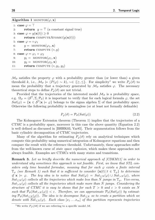
28 2. Temporal Logic
Algorithm 1 monitor(ϕ,x)
1: case ϕ = >2: return y = > (a constant signal true)3: case ϕ = y(x(t)) ≥ 04: return computeAtomic(y(x(t)))5: case ϕ = ϕ1
6: y = monitor(ϕ1,x)7: return compute (, y)8: case ϕ = ϕ1 ϕ2
9: y1 = monitor(ϕ1,x)10: y2 = monitor(ϕ2,x)11: return compute (, y1, y2)
Mϑ satisfies the property ϕ with a probability greater than (or lower than) a giventhreshold k, i.e., Mϑ |= (P (ϕ) ∼ k), ∼∈ ≥,≤. For simplicity1 we write Pϕ(ϑ) tomean the probability that a trajectory generated by Mϑ satisfies ϕ. The necessarytheoretical steps to define Pϕ(ϑ) are not trivial.
Provided that the trajectories of the interested model Mϑ is a probability space,e.g. Ωϑ = (ST,Σ,Pϑ) it is important to verify that for each logical formula ϕ, the setSat(ϕ) = x ∈ ST|x |= ϕ belongs to the sigma algebra Σ of that probability space.Otherwise the following probability is meaningless (or at least not formally definable)
Pϕ(ϑ) = Pϑ(Sat(ϕ)) (2.2)
The Kolmogorov Extension theorem (Theorem 1) implies that the trajectories of aCTMC is a probability space, moreover in this case the above quantity (Equation 2.2)is well defined as discussed in [BHHK03, Var85]. Their argumentation follows from thebasic cylindric decomposition of CTMC trajectories.
Many of the algorithm for estimating Pϕ(ϑ) rely on analytical techniques whichcompute this probability using numerical integration of Kolmogorov equations and thencompare the result with the reference threshold. Unfortunately, these approaches sufferfrom the well-known curse of state space explosion, which makes these approaches notalways feasible. Examples are CTMCs with many states and transitions.
Remark 3. Let us briefly describe the numerical approach of [CDKM11] in order tounderstand why sometimes this approach is not feasible. First, we know that STL con-siders only time bounded formulae, meaning that for each ϕ exists a finite intervalTϕ (see Remark 1) such that it is sufficient to consider x(t) | t ∈ Tϕ to determineif x |= ϕ. The key idea is to notice that Sat(ϕ) = Sat≤N (ϕ) ∪ Sat>N (ϕ), whereSat≤N (ϕ) collects all the trajectories which make less than N jumps in Tϕ. Vice-versa,Sat>N (ϕ) collects all the trajectories which make more than N jumps. Considering thestructure of CTMC it is easy to shows that for each T > 0 and ε > 0 exists an Nsuch that Pϑ(Sat>N (ϕ)) < ε. Therefore, we can approximate Pϑ(Sat(ϕ)) by estimat-ing Pϑ(Sat≤N (ϕ)). The idea is to decompose Sat≤N so to create a partition which wedenote with Sat≤N (ϕ). Each class [x1 . . . xm] of this partition represents trajectories
1We write Pϕ(M) if we are referring to a specific model M.

2.4. Statistical Model Checking 29
(xi, ti)i∈N such that ∀i ∈ N, ti < ti+1, tm ≤ max(Tϕ) and tm+1 > max(Tϕ) whichare different for the order of visited states. The next step is to filter out all the classeswhich do not contain trajectories which satisfy ϕ. For example, if ϕ = F[0,T ]f(s) > 0the algorithm will discard all the classes [x1 . . . xm] such that ∀i ≤ N, f(xi) ≤ 0, becauseindependently on t1t2 . . . tN we have that ((x1, t1), (x2, t2), . . . , (xN , tN )) 6|= ϕ. The re-maining classes, Sat≤N (ϕ), contain only trajectories which have at least a combinationof times (tii≤m) such that (xi, ti)i≤m |= ϕ, and m < N . Finally for each class ofSat≤N (ϕ) we can estimate S([x1 . . . xm]) ⊆ Tm which contains all the combination oftimes (tii≤m) such that (xi, ti)i≤m |= ϕ. Finally we can approximate Pϑ(Sat(ϕ))as follows:
Pϑ(Sat(ϕ)) ≈∑
[x1...xm]∈Sat≤N (ϕ)
m−1∏i=1
Rxi,xi+1
∫· · ·∫τ∈S([x1...xm])
e−E·τ (2.3)
where E = (E(x1), . . . , E(xm)) and τ = (t1, . . . , tm).The evaluation of the above formula 2.3 can be computational expensive. In order
to evaluate the multidimensional integral, first a decomposition of S([x1 . . . xm]) shouldbe provided. In [CDKM11] for example, a polyhedral decomposition is considered andthe integral is evaluated in each of these polyhedra. This decomposition and numericalintegration might be performed many times, considering that usually |Sat≤N (ϕ)| is ahigh value.
Statistical Model Checking (SMC) [YS06, ZPC13] have been introduced to solve theseissues. It relies on simulations which are faster than the numerical, symbolic algorithmused to achieve a precise evaluation of probability. Furthermore, it is a general approachwhich does not depend on the stochastic model class. For this reason, it is more suitablefor an industrial application.
We now describe the Bayesian Statistical approach appears in [ZPC13]. For a fre-quentist approach, we refer the reader to [YS06].
Bayesian SMC. There are two approaches: the Bayesian Interval Estimation (BIE),which estimates a confidence interval for the target probability p (i.e., the interval thatcontains p with at least a given confidence probability) and the Bayesian HypothesisTesting, which determines if p satisfies a given inequality within a given confidenceprobability. We describe the first approach. Let us consider a stochastic model, such asCTMC, and the Bernoulli random variable Xϕ (equal to 1 if a simulation trace satisfiesϕ, 0 otherwise).The goal of BIE is to estimate the probability p that Xϕ is equal to 1(i.e., p = P (Xϕ = 1)). This probability is well defined as already discussed in Section 1.2.The Bayesian approach assumes that p satisfies a prior probability distribution, whichreflects our previous experiences and beliefs about the model. In this case a reasonablechoice is the distribution Beta(α, β) which is defined in [0, 1] and depends on two shapeparameters α, β > 0. By varying the shape parameters, it is possible to approximatedifferent unimodal density distributions such as the uniform distribution in [0, 1] (α =β = 1) which is a reasonable choice with lack of prior information.
The cumulative distribution function F(α,β) of the beta distribution is defined for
30 2. Temporal Logic
each u ∈ [0, 1] as:
F(α,β)(u) =1
B(α, β)
∫ u
0
tα−1(1− t)β−1dt
where the beta function, B(α, β), is defined as:
B(α, β) =
∫ 1
0
tα−1(1− t)β−1dt
The beta distribution is the conjugate prior probability distribution for the Bernoulli,binomial, negative binomial and geometric distributions. That property, generally calledconjugate property, is appreciated in Bayesian statistics because it permits to avoidnumerical integration as described below.
Let us consider n simulations and h ≤ n successes (i.e., h = #(Xiϕ = 1)), if we
consider a beta prior distribution Beta(p | α, β) for the probability of p = P (Xϕ = 1),we easily obtain that the posterior probability of the Bernoulli i.i.d samples Xi
ϕi∈N is:
P (p | (h, n)) =P ((h, n) | p)Beta(p | α, β)
Z(h, n)= Beta(α+ h, β + n− h) (2.4)
where P ((h, n) | p) is a Bernoulli distribution and Z(h, n) =∫ 1
0P ((h, n) | p)Beta(p |
α, β)dp is the normalizing factor. Equation (2.4) is a consequence of the aforementionedconjugate property. The Bayesian approach works as follows. First a given confidenceprobability c (typically c = 0.99 or 0.95 ) and an admissible error δ ∈ (0, 1
2 ) are defined.At each simulation the number of successes is stored and the expectation (i.e., µ =h+α
n+α+β ) of the posterior probability is calculated. At this point the following probability
P(p ∈ (µ− δ, µ+ δ)
)= F(α+h,β+n−h)
(µ+
δ
2
)− F(α+h,β+n−h)
(µ− δ
2
)is evaluated and compared against the threshold c. Afterward, if this probability
is higher than c then the confidence probability has been reached, and the algorithmstops; otherwise, another simulation is performed, and the algorithm continues.
2.5 Statistics of Robustness
The probability of satisfaction for temporal logic (Equation 2.2) is an essential conceptin the field of stochastic system modeling. However, similarly to the robustness, whichhas been induced to overcome the limitations of Boolean semantics, we can consider theprobability distribution of robustness values [BBNS15].
Let us consider a set of models Mϑ, ϑ ∈ Θ, and the probability space Ωϑ =(ST,Σ,Pϑ) generated by their trajectories. We introduce the following set
Sat(ϕ | a, b) = x ∈ ST|%(ϕ,x, 0) ∈ [a, b]
and the real-valued random variable Rϕ(ϑ) with probability distribution

2.5. Statistics of Robustness 31
P (Rϕ(ϑ) ∈ [a, b]) = Pϑ(Sat(ϕ | a, b)) (2.5)
The well-foundedness of 2.5 obtained through the measurability of Sat(ϕ | a, b), i.e.,Sat(ϕ; a, b) ∈ Σ, is demonstrated in [BBNS15].
Useful statistics can be extracted from this probability distribution. A standardstatistics is the average robustness which was successfully applied in system design ofand biological processes such as Incoherent type 1 feed-forward loops and Schlogl system[BBNS15]. In Chapter 8, [BPS16], we also use the average robustness to solve a multi-objective design problem.


3Statistical Modeling
3.1 Gaussian Processes
Gaussian Processes (GP) [RW06] are non parametric Bayesian techniques used for clas-sification or regression. Thanks to their Bayesian nature GPs are particularly suitableto manage noise and encompass statistical beliefs about the considered dataset. Wenow introduce the GP approach to regression problem. For the classification problemwe refer the reader to [RW06].
Regression Task. We call training set a set of input-outputs pairs (xi, yi)i≤d, xi ∈Rn, yi ∈ R. We denote with X = (x1, . . . ,xd) and y = (y1, . . . ,yd), respectively, theinput and the output variables of the training set.
A regression problem consists in identifying a mathematical function f : Rn → Rsuch that the predicted values f(xi) are close as much as possible to the real valuesyi. The quality of this prediction is evaluated through a cost (or loss) function whichquantifies the distance between the predicted and the real values. Many regressiontechniques, such as linear and nonlinear least-squares approaches, try to minimize theoutcome of a proper loss function.
GPs use a different approach which relies on the probability framework. They com-bine a prior distribution over a set of possible regression functions with the informationprovided by the training set to choose a proper posterior distribution which is suitablefor estimation purposes.
Definition 14. Formally, a GP is a collection of random variables f(x) ∈ R indexed byan input variable x ∈ Rn such that every finite number of them have a joint Gaussiandistribution.
A GP f is uniquely determined by its mean and covariance function (called alsokernel) denoted respectively with m : Rn → R and k : Rn × Rn → R and defined as:
m(x) = E[f(x)]
k(x,x′) = E[(f(x)−m(x))(f(x′)−m(x′))]

34 3. Statistical Modeling
such that for every finite set of points (x1,x2, . . . ,xd):
f ∼ GP(m, k) ⇐⇒ (f(x1), f(x2), . . . , f(xn)) ∼ N (m,K) (3.1)
where m = (m(x1),m(x2), . . . ,m(xd)) is the vector mean and K ∈ Rn×n is the covari-ance matrix, such that Kij = k(xi,xj). A standard assumption is to consider (prior)Gaussian processes with a zero mean function. This is not a limitation because themean of the posterior distribution can be different from zero (see Equation 3.7).
A popular choice for the covariance function is the squared exponential covariancefunction
k(x, x′) = σ2 exp
(− (x− x′)2
λ2
)(3.2)
where length-scale, λ, is related to the minimum distance of the input space nec-essary to significantly change the value of the Gaussian process. The signal varianceσ2 represents the overall variance of the process. The reason for its importance is thefollowing property
Definition 15 (Universal Property). Let f be a continuous function defined in a com-pact domain of Rn. For every ε > 0 exists a sample function g from a GP with expo-nential kernel such that
‖f − g‖2 ≤ ε
where ‖ · ‖2 is the L2 norm.
The previous property is very important because makes the GPs a suitable priordistribution over continuous functions.
Learning Phase. The GP regression consists in modeling the relation between inputxi and output yi as noisy observations by setting yi = f(xi)+εi where the latent functionf is a Gaussian Process and the noises εi are sampled from a normal distribution, i.e.,εi ∼ N (0, σ2
n). The inference problem consists in identifying the best hyper-parameters(i.e., kf ) composing the covariance function of f , and the parameter of noise distributionσn, such that the model f(x) + ε approximates the training set at the best. This prob-lem is solved in the probabilistic framework through the maximization of the marginallikelihood defined as
p(y|X) =
∫p(y|f , X)︸ ︷︷ ︸likelihood
p(f |X)︸ ︷︷ ︸prior
df (3.3)
where f = (f(x1), . . . , f(xn)).Considering that the prior p(f |X) and the likelihood p(y|f , X) are Gaussian dis-
tributed, we obtain that the marginal likelihood p(y|X) is also Gaussian distributed. Itis convenient to introduce the log marginal likelihood (which is maximized in place ofthe marginal likelihood)
log p(y|X) = −1
2yT (K + σnI)−1y − 1
2|K + σnI| −
n
2log 2π (3.4)
where K is the m×m matrix, such that Kij = kf (xi,xj), and |K + σnI| is the deter-

3.2. Smoothed Model Checking 35
minant of K + σnI.
Posterior Prediction. Let us consider a GP f trained on a set (X,y). We arenaturally interested in computing the distribution of f on new points X∗ = (x∗1, . . . ,x
∗m).
The steps are the following:
1. From the GPs definition (Equation 3.1) we infer the conjugate prior
p(f∗, f | X∗, X) = N (0,K(X∗, X))
where f∗ = (f(x∗1), . . . , f(x∗m))) and K(X,X) is a (m+ d)× (m+ d) matrix of thecovariance evaluated at all the pairs of the test and the training set points.
2. The conjugate prior is combined with the likelihood and the following joint pos-terior distribution is obtained.
p(f∗, f | y, X∗, X) =1
Zp(f∗, f | X∗, X)p(y|f , X) (3.5)
where Z =∫p(f∗, f | X∗, X)p(y|f , X)df is the normalization factor.
3. Finally integrating over f from Equation 3.5, we obtain
p(f∗|y, X∗, X) =1
Z
∫p(f∗, f | X∗, X) p(y|f , X)df (3.6)
Equation 3.6 can be analytically computed and the result is the following Gaussiandistribution
p(f∗|y) = N (f∗, cov(f∗))
f∗ = K(X∗, X)[K(X,X) + σ2nI]−1y (3.7)
cov(f∗) = K(X∗, X∗)−K(X∗, X)[K(X,X) + σ2nI]−1K(X∗, X)
3.2 Smoothed Model Checking
Statistical Model Checking (SMC), as described in Section 2.4, can be applied only ifthe model is fully specified (i.e., the vector of parameters is fixed). In many domains,this limitation is too strict. Consider for example System Biology where in general manymodel parameters are not directly measurable, and a continuous set of possible values(i.e., an interval) is considered. Applying SMC, in this case, is not possible because aninfinite (or very large) number of SMC routine has to be performed (i.e., one for eachparameter value of the interval or in a discretized grid).
Smoothed Model Checking (smMC) [BMS16] is a novel technique which leverages thecontinuity of the satisfaction function (w.r.t the model parameters) and the regressionability of the Gaussian processes to estimate the probability of satisfaction Pϕ(ϑ) of aspecific property ϕ. It cast this task into a learning problem taking as input the truthvalue of ϕ for few simulations, (m << +∞), at different parameter vectors ϑ1, . . . , ϑn.

36 3. Statistical Modeling
As already discuss in Section 2.4, the satisfaction of the formula ϕ over a trajectorygenerated by the models Mϑ is a Bernoulli random variable with success probabilityPϕ(ϑ). Unfortunately, this function has a bounded codomain, and therefore it can notbe modeled through Gaussian processes. Smoothed Model Checking solves this issue byconsidering the inverse probit transformation Ψ: [0, 1]Θ → RΘ defined as follows
Ψ(Pϕ) ≡ f ⇐⇒ ∀ϑ ∈ Θ, Pϕ(ϑ) =
∫ f(ϑ)
−∞N (0, 1)dϑ
where N is the standard Gaussian distribution. The function gϕ(ϑ) = Ψ(fϕ(ϑ)) isa smooth real valued function of the model parameters and for this reason it can bemodeled with Gaussian processes.
Let us denote with O = [o1,o2, . . . ,on] the matrix whose rows oi are the Booleanm-vectors of the evaluations in ϑj . Hence, we have that each observation oi is anindependent draw from a Binomial(m,Pϕ(ϑj))). Smoothed Model Checking plugs theseobservations into a Bayesian inference scheme, assuming a prior p(f) for the latentvariable f . As f is a random function, one can take as a prior a GP, specifying its meanand kernel function, and then invoke Bayes theorem to compute the joint posteriordistribution of f at a prediction point ϑ∗ and at the observation points ϑ1, . . . , ϑn as
p(f(ϑ∗), f(ϑ1), . . . , f(ϑn) | o) =1
Zp(f(ϑ∗), f(ϑ1), . . . , f(ϑn))
n∏j=1
p(oj | f(ϑj)).
In the previous expression, on the right hand side, Z is a normalisation constant, whilep(f(ϑ∗), f(ϑ1), . . . , f(ϑn)) is the prior, which is Gaussian distribution with mean andcovariance matrix computed according to the GP. p(oj | f(ϑj)), instead, is the noisemodel, which in our case is given by a Binomial density. By integrating out the valueof the latent function at observations points in the previous expression, one gets thepredictive distribution
p(f(ϑ∗) | O) =
∫ n∏j=1
d(f(ϑj))p(f(ϑ∗), f(ϑ1), . . . , f(ϑn) | O).
The presence of a Binomial observation model makes this integral analytically in-tractable, and forces us to resort to an efficient variational approximation known asExpectation Propagation [BMS16, RW06]. The result is a Gaussian form for the predic-tive distribution for p(f(ϑ∗) | O), whose mean and δ-confidence region are then Probittransformed into [0, 1].
It is important to stress that the prediction of Smoothed Model Checking, being aBayesian method, depends on the choice of the prior. In case of Gaussian processes,choosing the prior means fixing a covariance function, which makes assumptions on thesmoothness and density of the functions that can be sampled by the GP. The squaredexponential covariance function (Equation 3.2) is dense in the space of continuous func-tions over a compact set [Ste01], hence it can approximate arbitrarily well the satisfactionprobability function. By setting its lengthscale via marginal likelihood optimization, weare picking the best prior for the observed data.

4Optimization
In this chapter we introduce the mathematical optimization, giving particular empha-sis to black box optimization. In many cases solving optimization problems with fewevaluations is a strict requirement. Therefore, we focus on active learning approacheswhich aim to reduce the number of evaluations needed to solve optimization tasks. Inparticular, we introduce the Gaussian process upper confidence bound algorithm whichis often used in black box optimization. Finally, we introduce the multi-objective opti-mization paradigm consisting in the simultaneous minimization of two or more objectivefunctions. This approach is used in many engineering fields, and it can be successfullyapplied in the model-based design of cyber-physical systems.
4.1 Bayesian Optimization
Definition 16. The general single-objective constrained optimization problem is definedas follows
fgl = minx∈D
f(x)
D =
m′⋂i=1
x ∈ Rn | ci(x) = 0
⋂ m⋂j=m′+1
x ∈ Rn | cj(x) ≥ 0
where the objective function f : Rn → R, n < ∞ has to be minimized and the deci-sion space D, where f takes values, has been defined by m′ equality constraints (i.e.,ci(x) = 0, i ∈ 1, . . . ,m′) and m − m′ inequality constraints (i.e., ci(x) ≥ 0, i ∈m′ + 1, . . . ,m) and 0 ≤ m′ < m < +∞.
fgl = f(x∗gl) and x∗gl are called, respectively, global minimum and global minimumpoint.
A point, xloc, is called local minimum point if
f(xloc) = minx∈Bδ(xloc)
f(x)
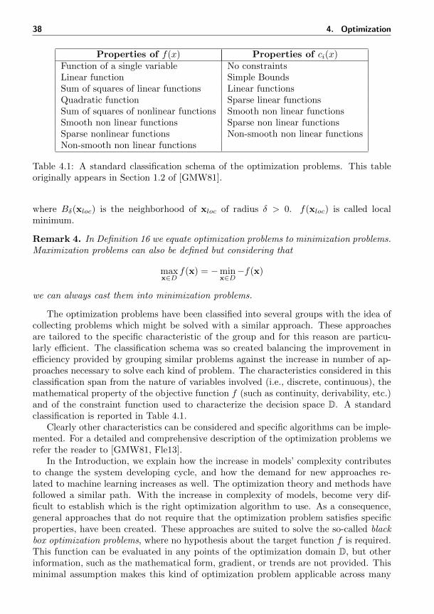
38 4. Optimization
Properties of f(x) Properties of ci(x)Function of a single variable No constraintsLinear function Simple BoundsSum of squares of linear functions Linear functionsQuadratic function Sparse linear functionsSum of squares of nonlinear functions Smooth non linear functionsSmooth non linear functions Sparse non linear functionsSparse nonlinear functions Non-smooth non linear functionsNon-smooth non linear functions
Table 4.1: A standard classification schema of the optimization problems. This tableoriginally appears in Section 1.2 of [GMW81].
where Bδ(xloc) is the neighborhood of xloc of radius δ > 0. f(xloc) is called localminimum.
Remark 4. In Definition 16 we equate optimization problems to minimization problems.Maximization problems can also be defined but considering that
maxx∈D
f(x) = −minx∈D−f(x)
we can always cast them into minimization problems.
The optimization problems have been classified into several groups with the idea ofcollecting problems which might be solved with a similar approach. These approachesare tailored to the specific characteristic of the group and for this reason are particu-larly efficient. The classification schema was so created balancing the improvement inefficiency provided by grouping similar problems against the increase in number of ap-proaches necessary to solve each kind of problem. The characteristics considered in thisclassification span from the nature of variables involved (i.e., discrete, continuous), themathematical property of the objective function f (such as continuity, derivability, etc.)and of the constraint function used to characterize the decision space D. A standardclassification is reported in Table 4.1.
Clearly other characteristics can be considered and specific algorithms can be imple-mented. For a detailed and comprehensive description of the optimization problems werefer the reader to [GMW81, Fle13].
In the Introduction, we explain how the increase in models’ complexity contributesto change the system developing cycle, and how the demand for new approaches re-lated to machine learning increases as well. The optimization theory and methods havefollowed a similar path. With the increase in complexity of models, become very dif-ficult to establish which is the right optimization algorithm to use. As a consequence,general approaches that do not require that the optimization problem satisfies specificproperties, have been created. These approaches are suited to solve the so-called blackbox optimization problems, where no hypothesis about the target function f is required.This function can be evaluated in any points of the optimization domain D, but otherinformation, such as the mathematical form, gradient, or trends are not provided. Thisminimal assumption makes this kind of optimization problem applicable across many

4.1. Bayesian Optimization 39
domains, where prior information on target functions is not known. In many practicalcases, the evaluation of the objective functions is also expensive. Consider, for example,the case of real experiments, physical simulations, or intensive computational modelswhere a single execution could require several hours. For this reason, a significant chal-lenge is to solve the optimization problem with few evaluations. Bayesian Optimization(BO) approaches are particularly suited for that task. These methods incorporate anatural trade-off between exploration and exploitation. The former is the ability ofsampling points from the optimization domain in a uniform setting, and the latter isthe ability to identify the promising area of the domain space where to concentrate thesampling.
A typical Bayesian optimization approach can be divided into the following threephases
Initial phase: an initial set of points is considered for evaluation. The purpose is tocollect a starting knowledge of the target function f to drive the further optimiza-tion algorithm. If prior knowledge of f is available, it can be considered, and acoherent sampling strategy adopted. On the other hand, if no prior knowledge isavailable, a uniform sampling strategy1, such as Latin Hypercube Sampling (LHS)[MBC79], Uniform Random Sampling or Full Factorial, is considered. All thenominated techniques are usually grouped under the umbrella of the Design ofExperiments (DOE) [Mon17].
Regression phase: a Bayesian regression technique (such as GPs) is used to derive amathematical representation of the underlined function f . This surrogate modelis trained on a training set generated during the initial phase.
Active learning phase: the surrogate model defined in the previous step is used tosample a point x which is the best candidate (up to the actual knowledge) tobe the global minimum. Afterwards, the function f = f(x) is evaluated and thecouple (x, f) is added to the training set of the surrogate model. The regressionand active learning phase are then iterated until a convergence criterion is reached.
4.1.1 Gaussian Processes Upper Confidence Bounds
Gaussian Processes Upper Confidence Bound (GP-UCB) is an interesting Bayesian op-timization approach particularly useful to minimize noisy function. Originally it wasproposed to solve the multi-armed bandit problem, a well-known problem of probabilitytheory, where a gambler has to decide which slot machines, in which order, and howmany times to play. The task of the gambler is the maximization of the reward pro-duced randomly by each machine. Mathematically this problem consists in maximizingan unknown reward function, f : Rn → R, by choosing, at each i-th round, a proper in-put point xi . The objective is to maximize
∑mi=1 f(xi) which is essentially the same of
discovering x∗ = arg maxx∈D f(x) as soon as possible. Let us consider the minimizationversion of the GP-UCB Algorithm.
The GP-UCB algorithm (Algorithm 2) takes as input an initial set of already evalu-ated points (i.e., trainingSet) and the Gaussian process (trained on the trainingSet)
1which is the most rationale option with this premise.
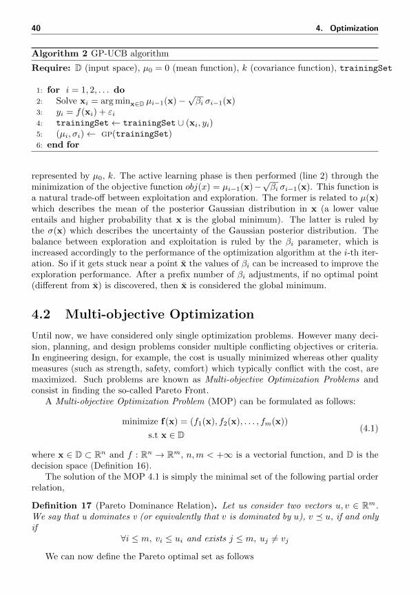
40 4. Optimization
Algorithm 2 GP-UCB algorithm
Require: D (input space), µ0 = 0 (mean function), k (covariance function), trainingSet
1: for i = 1, 2, . . . do2: Solve xi = arg minx∈D µi−1(x)−
√βi σi−1(x)
3: yi = f(xi) + εi4: trainingSet← trainingSet ∪ (xi, yi)5: (µi, σi)← gp(trainingSet)6: end for
represented by µ0, k. The active learning phase is then performed (line 2) through theminimization of the objective function obj(x) = µi−1(x)−
√βi σi−1(x). This function is
a natural trade-off between exploitation and exploration. The former is related to µ(x)which describes the mean of the posterior Gaussian distribution in x (a lower valueentails and higher probability that x is the global minimum). The latter is ruled bythe σ(x) which describes the uncertainty of the Gaussian posterior distribution. Thebalance between exploration and exploitation is ruled by the βi parameter, which isincreased accordingly to the performance of the optimization algorithm at the i-th iter-ation. So if it gets stuck near a point x the values of βi can be increased to improve theexploration performance. After a prefix number of βi adjustments, if no optimal point(different from x) is discovered, then x is considered the global minimum.
4.2 Multi-objective Optimization
Until now, we have considered only single optimization problems. However many deci-sion, planning, and design problems consider multiple conflicting objectives or criteria.In engineering design, for example, the cost is usually minimized whereas other qualitymeasures (such as strength, safety, comfort) which typically conflict with the cost, aremaximized. Such problems are known as Multi-objective Optimization Problems andconsist in finding the so-called Pareto Front.
A Multi-objective Optimization Problem (MOP) can be formulated as follows:
minimize f(x) = (f1(x), f2(x), . . . , fm(x))
s.t x ∈ D(4.1)
where x ∈ D ⊂ Rn and f : Rn → Rm, n,m < +∞ is a vectorial function, and D is thedecision space (Definition 16).
The solution of the MOP 4.1 is simply the minimal set of the following partial orderrelation,
Definition 17 (Pareto Dominance Relation). Let us consider two vectors u, v ∈ Rm.We say that u dominates v (or equivalently that v is dominated by u), v u, if and onlyif
∀i ≤ m, vi ≤ ui and exists j ≤ m, uj 6= vj
We can now define the Pareto optimal set as follows

4.2. Multi-objective Optimization 41
Definition 18. The Pareto optimal Set (PS) is the subset of the decision space D definedas
PS = x ∈ D | 6 ∃y ∈ D, f(y) f(x)
and the Pareto Front (PF) is the subset of the codomain of f , defined as
PF = f(x) |x ∈ PS
Informally, the Pareto optimal set is the best compromise that can be obtained bymaximizing or minimizing a set of functions on the same domain set. A point belongsto it if an improvement of an objective function causes another objective function todeteriorate (i.e., decreases its value).
4.2.1 Algorithms and Approaches
Many approaches have been developed to solve MOP, we refer the reader to the followingsurveys [ZQL+11, MA04] and books [Mie99, Deb01]. In this section, we describe twoapproaches: the wighted sum and non-dominated sorting genetic algorithm which is oneof the most used Evolutionary Algorithm (EA).
Weighted Sum Approach (WSA). We present this approach for three reasons.First, it is still used to solve simple MOP, second, it is the simplest approach thatmight come to mind, and third its main weakness justify the existence of more ad-vanced multi-objective approaches. The idea of WSA is straightforward and consists inconsidering a unique function by a linear combination of the objective functions (i.e.,F (x) =
∑nj=1 αjfj(x), where ∀i ≤ n, αi ≥ 0, and
∑ni=1 αi = 1). Fixed α, the mini-
mization of the referred function means to discover a single point of the Pareto front.As a consequence, multiple single objective problems have to be solved to estimatethe whole Pareto front. The main weakness of WSA is its inability to approximatenon-convex Pareto front.
Evolutionary Algorithms (EA). Evolutionary Algorithms are population-basedmeta-heuristic algorithms inspired by the natural evolution of species, where the ge-netic heritage of populations improves during time evolution. Genetic Algorithms(GA) are particular kind of EA, largely used in engineering fields, where each designx = (x1, . . . , xn) represents a chromosome, formed by genes (xi, i ≤ n). Chromosomesare modified by two genetic operators: crossover and mutation. The first is a binary op-erator which gets two chromosomes and generates a new one by mixing their genes. Thesecond is a unary operator which acts on a single chromosome by randomly muting itsgenes (see Figure 4.2). Mathematically crossover and mutation are related, respectively,to exploitation and exploration.
Genetic algorithms execute a predefined number of cycles (or iterations), usuallycalled generations, where a fixed number of designs (for example N) are evaluated andsorted accordingly to a specific ranking function. Afterward, the genetic operators haveperformed on these designs accordingly to their ranking score (i.e., designs with a higherrank are considered with a higher frequency) and a new generation of design is generated.The algorithm then iterates until a threshold number of generations is reached.

42 4. Optimization
Figure 4.1: This is an approximation of the Pareto front of a standard bi-objective op-timization test case called TNK, which has been obtained employing NSGA-II (originalFigure in [DAPM02]). In this case, the WSA approach will be unable to identify pointsin the middle of the Pareto front and will identify only points around (0, 1) and (1, 0).
Non-dominated Sorted Genetic Algorithm (NSGA-II) is a well known GA introducedin 2000 by K. Deb [DAPM02]. It is an improvement of NSGA ([SD94]) algorithm ob-tained by the implements of three techniques: non-dominated sorting, crowding distanceand elitism .
Non-dominated sorting is a ranking function based on the Pareto dominance relation(Definition 17). This ranking function splits a finite set of designs in chunks: the firstchunk includes the non-dominated points, the second considers the points dominatedonly by the first chunks, and so on. The points contained in each chunk, which bydefinition cannot be ordered by the Pareto dominance relation, are sorted by using thecrowding distance.
The crowding distance is a metric used to maximize the uniform displacement of de-signs towards the Pareto front. Consider a set of designs of an n-dimensional MOP (i.e.,a MOP with n objective functions). The 2n extreme points x−i = minx∈D fi(x), x+
i =maxx∈D fi(x), i ≤ n have a fixed crowding distance of +∞ (i.e., c(x−i ) = c(x+
i ) =+∞, ∀i ≤ n). For any other point x, and for each objective fi, the adjacent points x+
i
and x−i to x are defined as follows
x+i = arg min
x′∈D∩x′ | fi(x′)>fi(x)fi(x
′)
x−i = arg maxx′∈D∩x′ | fi(x′)<fi(x)
fi(x′)
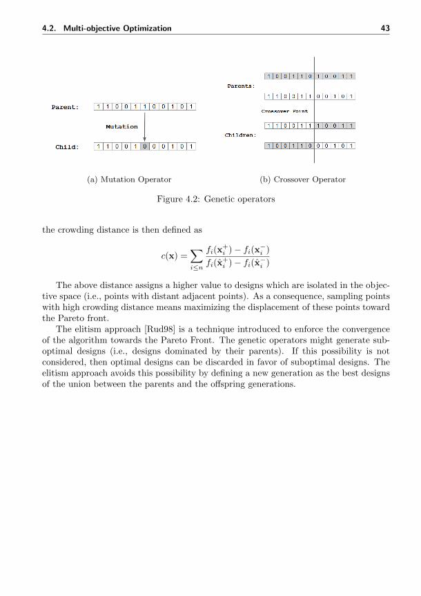
4.2. Multi-objective Optimization 43
(a) Mutation Operator (b) Crossover Operator
Figure 4.2: Genetic operators
the crowding distance is then defined as
c(x) =∑i≤n
fi(x+i )− fi(x−i )
fi(x+i )− fi(x−i )
The above distance assigns a higher value to designs which are isolated in the objec-tive space (i.e., points with distant adjacent points). As a consequence, sampling pointswith high crowding distance means maximizing the displacement of these points towardthe Pareto front.
The elitism approach [Rud98] is a technique introduced to enforce the convergenceof the algorithm towards the Pareto Front. The genetic operators might generate sub-optimal designs (i.e., designs dominated by their parents). If this possibility is notconsidered, then optimal designs can be discarded in favor of suboptimal designs. Theelitism approach avoids this possibility by defining a new generation as the best designsof the union between the parents and the offspring generations.


IIContributions


5Signal Convolution Logic
In this chapter, we introduce Signal Convolution Logic (SCL), a logical framework whichis able to express non-functional requirements. The fundamental idea of this logic is toconsider a modal operator, 〈kT , p〉ϕ, that we call the convolution operator, which de-pends on a non-linear kernel function kT , and asserts that the convolution betweenthe kernel and the signal (i.e., the satisfaction of ϕ) is above a given threshold p.This operator allows us to specify queries about the fraction of time a specific prop-erty is satisfied, possibly weighting unevenly the satisfaction in a given time intervalT = [T0, T1], T0, T1 ∈ R+
0 , e.g., allowing to distinguish traces that satisfy a propertymore at the beginning or the end of T . We equip the logic with a Boolean semantics,and then define a quantitative semantics, proving its soundness and correctness concern-ing the former. Similarly to Signal Temporal Logic (STL), our definition of quantitativesemantics permits to quantify the maximum allowed uniform translation of the signals,preserving the true value of the formula. We also show that SCL is an extension of thefragment of STL restricted to finally and globally modalities. We then discuss mon-itoring algorithms for both semantics, in particular presenting an efficient monitoringalgorithm for the Boolean semantics and an arbitrary kernel function. We finally showthe logic at work to monitor an artificial pancreas device releasing insulin in patientsaffected by type-I diabetes.
Motivation. Despite STL is a powerful specification language, it does not come with-out limitations. An essential type of properties that STL cannot express is the non-functional requirements related to the percentage of time-specific events happen. Theglobally and finally operators of STL can only check if a condition is true for all timeinstants or in at least one time instant, respectively. There are many real situationswhere these conditions are too strict, where we could be interesting to describe a prop-erty that is in the middle between eventually and globally. We now give three exampleswhere SCL can be useful.
• Time duration. Consider for instance a medical cyber-physical system, e.g., adevice measuring glucose level in the blood to release insulin in diabetic patients.In this scenario, we need to check if glucose level is above (or below) a given

48 5. Signal Convolution Logic
(a) (b)
Figure 5.1: (a) A graphical representation of the property ϕ : G(t) ≥ 180 for at least12.5% in [0,24h], meaning that the concentration of glucose has to be greater than 180for at least 3h in 24h. (b) A graphical representation of the property ψ : G(t) > 70 forat least 95% in [0,24h]. (both) The bars on the right represent the percentage of timethe property is satisfied. At the bottom of each graph we highlight (dark red) the timewhere the atomic predicates are true.
threshold for a certain amount of time, to detect critical settings. Short periodsof hyperglycemia (high level of glucose) are not dangerous for the patients. Anunhealthy scenario is when the patient remains in hyperglycemia for more than 3hours during the day, i.e., for 12.5% of 24 hours (see Figure 5.1a). STL cannotspecify this property.
• Noisy measurement. A second issue is that often such measurements are noisy,and measurement errors or tiny random fluctuations due to environmental factorscan easily violate (or induce the satisfaction) of a property. One way to approachthis problem is to filter the signal to reduce the impact of noise, in a way that isconsistent with the property at hand. This requires a signal pre-processing phase,which may, however, alter the signal introducing spurious behaviors. Anotherpossibility instead is to ask that the property is true for at least 95% of operatingtime, rather than for 100% of the time, this requirement can be seen as a relaxedglobally condition (see Figure 5.1b).
• Inhomogeneous time. Finally, there are situations when it is difficult to pre-cisely specify the time intervals of temporal operators. As an example, whilemeasuring the glucose level in blood, it is more dangerous if the glucose level ishigh just before a meal. To capture this requirement, one could give differentweight to the satisfiability of the formula at the beginning or the end or in themiddle of a time interval, i.e., to consider the inhomogeneous temporal satisfactionof a formula. This is also not possible in STL.
5.1. Signal Convolution Logic 49
Related Work. In this paragraph, we discuss different extensions of STL, in partic-ular analyzing different notions of robustness. In Section 2.2 we already described thequantitative semantics and its benefits from a general point of view. We also introduceda quantitative semantics called robustness semantics [FP09, DM10]. Other quantitativesemantics are discussed below. In [DM10] the authors consider both the spatial robust-ness and also the displacement of a signal in the time domain (temporal robustness).These semantics, since are related to the L∞ topology, are very sensitive to glitches (i.e.,sporadic peaks in the signals due to measurement errors). This limitation affects the useof this semantics in the model predictive control of noisy systems such as robot plan-ning and autonomous driving. In these contexts Probabilistic Signal Temporal Logic(PrSTL) [SK16] and Chance-Constrained Signal Temporal Logic (C2CTL) [JRSS18]have been proposed.
Rodionova et al. [RBNG17] proposed a quantitative semantics based on filtering.More specifically they provide a quantitative semantics for the positive normal formfragment of STL which measures the number of times a formula it is satisfied within aninterval associating to it different types of kernels. One limitation of this approach isthat, by restricting the quantitative semantics to the positive normal form they neededto give up the duality property between the eventually and the globally operators, whichinstead we can keep in our approach.
In [AH15], Akazaki et al. have extended the syntax of STL by introducing averagedtemporal operators which enable the possibility to consider time not homogeneously.Their quantitative semantics expresses the preference that a specific requirement occursas earlier as possible in a given range of time. However, this time inhomogeneity can beevaluated only for the quantitative semantics. The new operators, at the Boolean level,are equal to the classic until (since) operators. Furthermore, they can consider only thisspecific type of time inhomogeneities (early as possible, for as long as possible) and acombination of them with classic temporal STL operators.
Note that defining a new quantitative semantics has an intrinsic limitation. Evenif the robustness can help the system design or the falsification process by guidingthe underline optimization, it cannot be used at a syntax level. It means that wecannot write logical formulae which predicate about the property. For example, evenif we introduce a quantitative semantics which measures how many times a propertyis satisfied, as in [RBNG17], we cannot write a formula which quantifies it, e.g., thepropriety has to be satisfied in at least the 50% of interval T, but we can only measurethe percentage of time the property has been verified.
5.1 Signal Convolution Logic
In this section we present the syntax and semantics of Signal Convolution Logic (SCL),also discussing its soundness, correctness, and finally commenting on expressiveness ofthe logic.
Let us briefly introduce the notions needed later in this chapter: kernel and convo-lution.
Definition 19 (Bounded Kernel). Let T ⊂ R be a closed interval. We call bounded
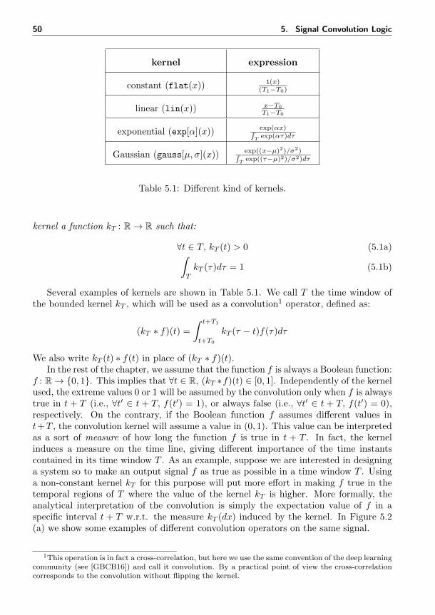
50 5. Signal Convolution Logic
kernel expression
constant (flat(x)) 1(x)(T1−T0)
linear (lin(x)) x−T0
T1−T0
exponential (exp[α](x)) exp(αx)∫T
exp(ατ)dτ
Gaussian (gauss[µ, σ](x)) exp((x−µ)2)/σ2)∫T
exp((τ−µ)2)/σ2)dτ
Table 5.1: Different kind of kernels.
kernel a function kT : R→ R such that:
∀t ∈ T, kT (t) > 0 (5.1a)∫T
kT (τ)dτ = 1 (5.1b)
Several examples of kernels are shown in Table 5.1. We call T the time window ofthe bounded kernel kT , which will be used as a convolution1 operator, defined as:
(kT ∗ f)(t) =
∫ t+T1
t+T0
kT (τ − t)f(τ)dτ
We also write kT (t) ∗ f(t) in place of (kT ∗ f)(t).In the rest of the chapter, we assume that the function f is always a Boolean function:
f : R→ 0, 1. This implies that ∀t ∈ R, (kT ∗f)(t) ∈ [0, 1]. Independently of the kernelused, the extreme values 0 or 1 will be assumed by the convolution only when f is alwaystrue in t + T (i.e., ∀t′ ∈ t + T, f(t′) = 1), or always false (i.e., ∀t′ ∈ t + T, f(t′) = 0),respectively. On the contrary, if the Boolean function f assumes different values int+T , the convolution kernel will assume a value in (0, 1). This value can be interpretedas a sort of measure of how long the function f is true in t + T . In fact, the kernelinduces a measure on the time line, giving different importance of the time instantscontained in its time window T . As an example, suppose we are interested in designinga system so to make an output signal f as true as possible in a time window T . Usinga non-constant kernel kT for this purpose will put more effort in making f true in thetemporal regions of T where the value of the kernel kT is higher. More formally, theanalytical interpretation of the convolution is simply the expectation value of f in aspecific interval t + T w.r.t. the measure kT (dx) induced by the kernel. In Figure 5.2(a) we show some examples of different convolution operators on the same signal.
1This operation is in fact a cross-correlation, but here we use the same convention of the deep learningcommunity (see [GBCB16]) and call it convolution. By a practical point of view the cross-correlationcorresponds to the convolution without flipping the kernel.

5.1. Signal Convolution Logic 51
5.1.1 Syntax and Semantics
The atomic predicates of SCL are inequalities on a set of real-valued variables, i.e. of theform µ(s):=[g(s) ≥ 0], where g : S → R is a continuous function, s ∈ S and consequentlyµ : S → >,⊥. The formulae LSCL of SCL are defined by the following grammar
ϕ := ⊥ |> |µ | ¬ϕ |ϕ ∨ ϕ | 〈kT , p〉ϕ, (5.2)
where µ are atomic predicates as defined above, kT is a bounded kernel and p ∈ [0, 1].SCL introduces a novel modal operator 〈kT , p〉ϕ (in fact, a family of them) defined para-metrically w.r.t. a kernel kT and a threshold p. This operator specifies the probabilityof ϕ being true in T , computed w.r.t. the probability measure kT (ds) of T . The choiceof different types of kernel will give rise to different kind of operators: a constant kernelwill measure the fraction of time ϕ is true in T , while an exponentially decreasing kernelwill concentrate the focus on the initial part of T . We interpret the SCL formulae oversignals.
Before describing the semantics, we give a couple of examples of SCL properties andtheir natural language expression. Considering again the glucose scenario presented inSection 5. The properties in Figure 5.1 are specified in SCL as
ϕ1 : 〈flat[0,24h], 0.125〉 (G(t) ≥ 180)
ϕ2 : 〈flat[0,24h], 0.95〉 (G(t) ≥ 50)
ϕ3 : 〈exp[0,8h], 0.95〉 (G(t) ≥ 180)
where ϕ1 means the level of glucose (G) is higher than 180 for more than 3 hoursand ϕ2 mean that the the same level is higher than 50 for more than 95% of the day(i.e., 24h), (see Figure 5.1). ϕ3 leverages an exponential increasing kernel to describethe more dangerous situation of high glucose close (in time) to a meal .
Let us introduce the Boolean and quantitative semantics. Consider that tempo-ral operators 〈kT , p〉 are time-bounded, and for this reason, time-bounded signals aresufficient to assess the truth of every formula.
Definition 20 (Boolean Semantics). Given a signal s ∈ ST, the Boolean semanticsχ : ST × T× LSCL → 0, 1 is defined recursively by:
χ(s, t, µ) = 1 ⇐⇒ µ(s(t)) = > where µ(X) ≡ [g(X) ≥ 0] (5.3a)
χ(s, t,¬ϕ) = 1 ⇐⇒ χ(s, t, ϕ) = 0 (5.3b)
χ(s, t, ϕ1 ∨ ϕ2) = max(χ(s, t, ϕ1), χ(s, t, ϕ2)) (5.3c)
χ(s, t, 〈kT , p〉ϕ) = 1 ⇐⇒ kT (t) ∗ χ(s, t, ϕ) ≥ p (5.3d)
The atomic propositions µ are inequalities over the signal’s variables. The semanticsof negation and conjunction are the same as classical temporal logics. The semantics of〈kT , p〉ϕ requires to compute the convolution of kT with the truth value χ(s, t, ϕ) of theformula ϕ as a function of time, seen as a Boolean signal, and compare it with the thresh-old p. An example of the Boolean semantics can be found in Figure 5.2(a - bottom)where four horizontal bars visually represent the validity of ψ = 〈k[0,0.5], 0.5〉(s > 0), for

52 5. Signal Convolution Logic
4 different kernels k (one for each bar). We can see that the the only kernel for whichχ(s, ψ) = 1 is the exponential increasing one, i.e., k = exp[3].
Definition 21 (Quantitative semantics). The quantitative semantics % : ST × T ×LSCL → R ∪ −∞,+∞ is defined as follows:
%(s, t,>) = +∞ (5.4a)
%(s, t, µ) = g(s(t)) where g is such that µ(s) ≡ [g(s) ≥ 0] (5.4b)
%(s, t,¬ϕ) = −%(ϕ, s, t) (5.4c)
%(s, t, ϕ1 ∨ ϕ2) = max(%(ϕ1, s, t), %(ϕ2, s, t)) (5.4d)
%(s, t, 〈kT , p〉ϕ) = supr ∈ R | kT (t) ∗ [%(s, t, ϕ) > r] > p (5.4e)
where in equation (5.4e) we use the Iverson brackets [Knu92], i.e., [%(s, t, ϕ) > r] is afunction of t which assumes 1 if %(s, t, ϕ) > r, 0 otherwise.
Intuitively the quantitative semantics of a formula ϕ w.r.t. a primary signal sdescribes the maximum allowed uniform translation of the secondary signals g(s) =(g1(s), . . . , gn(ϕ)(s)) in ϕ preserving the truth value of ϕ. Stated otherwise, a robust-ness of r for ϕ means that all signals s′ such that ‖g(s′) − g(s)‖∞ ≤ r will result inthe same truth value for ϕ: χ(s, t, ϕ) = χ(s′, t, ϕ). Figure 5.2(b) shows this geometricconcept visually. Let us consider the formula ϕ = 〈k[0,3], 0.3〉(s > 0), k a flat kernel. Asignal s(t) satisfies the formula if it is greater than zero for at most the 30% of the timeinterval T = [0, 3]. The robustness value corresponds to how much we can translate s(t)s.t. the formula is still true, i.e., r s.t. s(t) − r still satisfies ϕ. In the figure, we cansee that r = 0.535. The formal justification of it is rooted in the correctness theorem(Theorem 3).
5.1.2 Soundness and Correctness
We turn now to discuss soundness and correctness of the quantitative semantics withrespect to the Boolean one.
Theorem 2 (Soundness Property). The quantitative semantics is sound with respect tothe Boolean semantics:
%(s, t, ϕ) > 0 =⇒ (s, t) |= ϕ
%(s, t, ϕ) < 0 =⇒ (s, t) 6|= ϕ
Proof. The demonstration is by induction on the structure of the formula. The sound-ness holds for the atomic predicates and Boolean operators: this is the proof of sound-ness for classic robustness, see [DM10, FP09]. Consider then the formula 〈kT , p〉ϕ. If%(s, t, 〈kT , p〉ϕ) ≥ 0, by Definition 21 (Equation 5.4e) we have that kT (t) ∗ [%(s, t, ϕ) >0] > p. By the inductive hypothesis, ϕ satisfies the soundness property, hence it followsthat kT (t) ∗ χ(s, t, ϕ) ≥ p, i.e., (s, t) |= 〈kT , p〉ϕ.
Theorem 3 (Correctness Property). The quantitative semantics % satisfies the correct-ness property with respect to the Boolean semantics if and only if, for each formula ϕ,
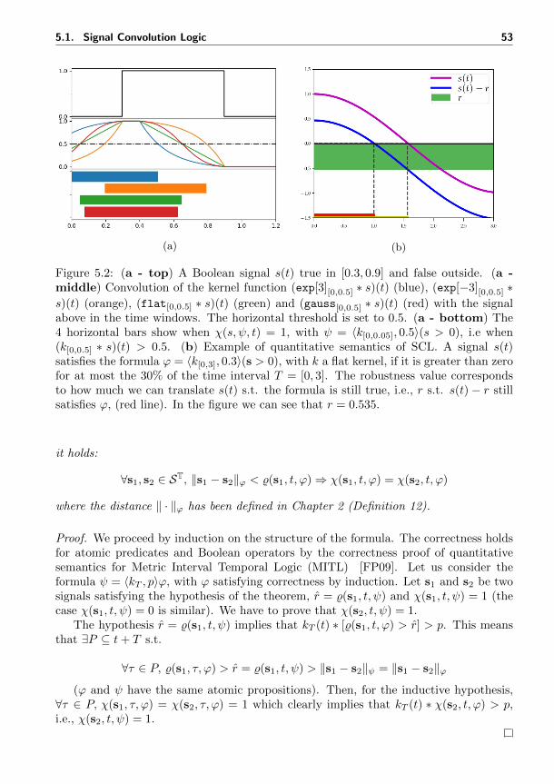
5.1. Signal Convolution Logic 53
(a) (b)
Figure 5.2: (a - top) A Boolean signal s(t) true in [0.3, 0.9] and false outside. (a -middle) Convolution of the kernel function (exp[3][0,0.5] ∗ s)(t) (blue), (exp[−3][0,0.5] ∗s)(t) (orange), (flat[0,0.5] ∗ s)(t) (green) and (gauss[0,0.5] ∗ s)(t) (red) with the signalabove in the time windows. The horizontal threshold is set to 0.5. (a - bottom) The4 horizontal bars show when χ(s, ψ, t) = 1, with ψ = 〈k[0,0.05], 0.5〉(s > 0), i.e when(k[0,0.5] ∗ s)(t) > 0.5. (b) Example of quantitative semantics of SCL. A signal s(t)satisfies the formula ϕ = 〈k[0,3], 0.3〉(s > 0), with k a flat kernel, if it is greater than zerofor at most the 30% of the time interval T = [0, 3]. The robustness value correspondsto how much we can translate s(t) s.t. the formula is still true, i.e., r s.t. s(t)− r stillsatisfies ϕ, (red line). In the figure we can see that r = 0.535.
it holds:
∀s1, s2 ∈ ST, ‖s1 − s2‖ϕ < %(s1, t, ϕ)⇒ χ(s1, t, ϕ) = χ(s2, t, ϕ)
where the distance ‖ · ‖ϕ has been defined in Chapter 2 (Definition 12).
Proof. We proceed by induction on the structure of the formula. The correctness holdsfor atomic predicates and Boolean operators by the correctness proof of quantitativesemantics for Metric Interval Temporal Logic (MITL) [FP09]. Let us consider theformula ψ = 〈kT , p〉ϕ, with ϕ satisfying correctness by induction. Let s1 and s2 be twosignals satisfying the hypothesis of the theorem, r = %(s1, t, ψ) and χ(s1, t, ψ) = 1 (thecase χ(s1, t, ψ) = 0 is similar). We have to prove that χ(s2, t, ψ) = 1.
The hypothesis r = %(s1, t, ψ) implies that kT (t) ∗ [%(s1, t, ϕ) > r] > p. This meansthat ∃P ⊆ t+ T s.t.
∀τ ∈ P, %(s1, τ, ϕ) > r = %(s1, t, ψ) > ‖s1 − s2‖ψ = ‖s1 − s2‖ϕ(ϕ and ψ have the same atomic propositions). Then, for the inductive hypothesis,
∀τ ∈ P, χ(s1, τ, ϕ) = χ(s2, τ, ϕ) = 1 which clearly implies that kT (t) ∗ χ(s2, t, ϕ) > p,i.e., χ(s2, t, ψ) = 1.

54 5. Signal Convolution Logic
5.1.3 Expressiveness
We show that SCL is more expressive than the fragment of STL composed of the logicalconnectivities and the eventually F and globally G temporal operators, i.e., STL(F,G).
First of all, globally is easily definable in SCL. Take any kernel kT , and observe thatGTϕ ≡ 〈kT , 1〉ϕ which results considering that
(s, t) |= 〈kT , 1〉ϕ ⇐⇒ kT (t) ∗ χ(s, t, ϕ) = 1
which holds only if ϕ is true in the whole interval T . This statement is valid onlyif we restrict ourselves to Boolean signals of finite variation, as for [MN04], which arechanging truth value a finite amount of times and are never true or false in isolatedpoints: in this way we do not have to care what happens in sets of zero measure. Witha similar restriction in mind, we can define the eventually, provided we can check that
kT (t) ∗ χ(s, t, ϕ) > 0
To see how this is possible, start from the fundamental equation kT (t)∗χ(s, t,¬ϕ) =1− kT (t) ∗ χ(s, t, ϕ). By applying 5.3d and 5.3b we easily get χ(s, t,¬〈kT , 1− p〉¬ϕ) =1 ⇐⇒ kT (t) ∗χ(s, t,¬ϕ) < 1− p ⇐⇒ kT (t) ∗χ(s, t, ϕ) > p. For compactness we write〈kT , p〉∗ = ¬〈kT , 1− p〉¬, and thus define the eventually modality as FTϕ ≡ 〈kT , 0〉∗ϕ.Furthermore, consider the uniform kernel flatT : a property of the form 〈flatT , 0.5〉ϕ,requesting ϕ to hold at least half of the time interval T , cannot be expressed in STL,showing that SCL is more expressive than STL(F,G).
5.2 Monitoring Algorithm
We now provide two offline monitor algorithms for the Boolean semantics of SCL formu-lae (approach I and approach II) and a monitor algorithm for the quantitative semantics.
Boolean monitoring: approach I. The first method we present works for a sub-class of kernels (mostly used in practice), satisfying a semigroup property. The secondmethod, which is an extension of the first one, instead, works for generic kernels.
Consider the following SCL formula 〈k[T0,T1], p〉ϕ and a Boolean signal s, we areinterested in computing χ(s, t, 〈k[T0,T1], p〉ϕ) = (H(t)− p ≥ 0), as a function of t, whereH is the following convolution function
H(t) = kT (t) ∗ χ(s, t, ϕ) =
∫ t+T1
t+T0
k[T0,T1](τ − t)χ(s, τ, ϕ)dτ (5.5)
It follows that the efficient monitoring of the Boolean semantics of SCL is linked tothe efficient evaluation of H(t)−p, which is possible if exists h sufficiently big such thatH(t+h) can be computed by reusing the value of H(t) previously stored. If the kernel isa constant function (i.e., ∀t ∈ T, k(t) = k0), linear (i.e., ∀t0, t1 ∈ T, k(t0 + t1) = k(t0) +k(t1)), or exponential (i.e., it satisfies the semigroup property: ∀t0, t1 ∈ T, k(t0 + t1) =k(t0) · k(t1)), this can be efficiently done:
Constant: Hconst(t+ h)− p = H(t)− p+ IkT (t+ T1, t+ T1 + h)− IkT (t+ T0, t+ T0 + h).

5.2. Monitoring Algorithm 55
Linear: Hlin(t + h) − p = H(t) − p + IkT (t+ T1, t+ T1 + h) − IkT (t+ T0, t+ T0 + h) +kT (−h)Hconst(t+ h).
Exponential: Hexp(t+h)−p = H(t)−p+IkT (t+ T1, t+ T1 + h)−IkT (t+ T0, t+ T0 + h)+p(1− e−αh).
where IkT (a, a+ h) =∫ a+h
akT (τ − a)χ(s, τ, ϕ)dτ .
These relationships can be easily exploited to obtain an algorithm that computesthe values of H(t) − p. The computation can be optimized by suitably tracking thetimes in which the signal χ(s, τ, ϕ) switches values. The algorithm is fully reported inthe following subparagraph.
The Algorithm. We now describe the monitoring algorithm for the convolutionformula χ(s, t, 〈k[T0,T1], p〉ϕ). The monitors for the others formulae are described in[DFM13]. The Boolean signal can be decomposed (see [MN04]) in a sequence of disjointunitary signals U = U1 + · · ·+Un s.t. each U i(t) is true only in a single interval of time[U i0, U
i1], false outside. We denote with subscript 0 the lower bounds and with subscript
1 the upper bound, whereas the superscript i indicates a specific unitary signal.The key idea consists in monitoring H by choosing h such that between t and t+h the
Boolean signal χ(s, t, ϕ) assumes a constant value (i.e., 1 or 0) in [t+T0, t+T0 +h] and[t+T1, t+T1 +h], respectively. Therefore, IkT can be easily computed as the differenceof the primitive of kT evaluated in 0, h and T1−T0−h, T1−T0 multiplied by the constantvalue assumes by the signal. For example if χ(s, τ, ϕ) = 1 if τ ∈ [t+ T0, t+ T0 + h] thanIkT (t + T0, t + T0 + h) = KT (h) − KT (0) where KT is the primitive of the kernel kT .Let us describes this procedure (Algorithm 3) in details. The algorithm takes as inputsthe interval [t, te] where we want to monitor χ(s, t, 〈k[T0,T1], p〉ϕ), the kernel k[T0,T1],the Boolean signal χ(s, t, ϕ), and the threshold p ∈ [0, 1]. At line 1 the Boolean signalχ(s, t, ϕ) is decomposed into a sequence of unitary signals as explain above, afterward(line 2) the algorithm initializes H(t) to (k[T0,T1]∗U)(t), which is evaluated by a standardintegration technique, and the value of init and end, which are two integers pointing tothe first unitary signal (i.e, U init) such that U init1 > t+ T0, and the last unitary signal(i.e., Uend ) such that Uend0 ≤ t+T1. A while cycle (line 4−32) performs the integrationstep until the convolution is evaluated on the entire interval [t, te]. Depending on thecases, if the bounds of the convolution window (i.e., t + T0 and t + T1) intersect anunitary signal composing U , four different integration strategies are performed (blocksat lines: 5 − 8, 9 − 12, 13 − 16, 17 − 20), and the proper value of the integration step(i.e., h) which avoids discontinuity is also evaluated (lines: 6, 10, 14, 18). The value ofh, indeed, implies that between t and t + h no new intersection of unitary signals U i
with the convolution windows occurs. Afterward, the finite difference H(t+h)−H(t) isstored in ∆H and the integration step (H(t+ h) = H(t) + ∆H) is performed (line 21).The value of this finite difference depends on the particular kernel used. It involves theevaluation of the primitive of kT which we denote by capital letter KT plus other terms(i.e, zero for the flat kernel, p(1− e−αh) for the exponential kernel, etc.).
If during this integration step H(t)−p changes sign (line 22), then the exact momentis evaluated by means of a root finding routine (line 23). These time values define theBoolean semantics of χ(s, t, 〈k[T0,T1], δ, p〉ϕ). Finally, in lines 25 − 30, the values of t,init and end are updated and the cycle continues.

56 5. Signal Convolution Logic
Algorithm 3 (Approach I) Monitoring Algorithm: χ(s, t, 〈k[T0,T1], p〉ϕ)
Require: t, te, k[T0,T1], χ(s, t, ϕ), p1: U ← Decompose(χ(s, t, ϕ))2: H(t) = (k[T0,T1] ∗ U)(t)3: initialize(init, end)
4: while (t < te) do5: if (t+ T0 ∈ U init and t+ T1 ∈ Uend) then6: h← min(t+ T0 − U init1 , Uend1 − t− T1)7: ∆H ← KT (h)−KT (0) +KT (T1 − T0)−KT (T1 − T0 − h) + other terms.8: end if9: if (t+ T0 ∈ U init and t+ T1 6∈ Uend) then
10: h← min(t+ T0 − U init1 , Uend+10 − t− T1)
11: ∆H ← KT (h)−KT (0) + other terms.12: end if13: if (t+ T0 6∈ U init and t+ T1 ∈ Uend) then14: h← min(Uend1 − t− T1, U
init0 − t− T0)
15: ∆H ← KT (T1 − T0)−KT (T1 − T0 − h) + other terms.16: end if17: if (t+ T0 6∈ U init and t+ T1 6∈ Uend) then18: h← min(U init0 − t− T0, U
end+10 − t− T1)
19: ∆H ← other terms.20: end if
21: H(t+ h)← H(t) + ∆H22: if (H(t+ h)− p) · (H(t)− p) ≤ 0) then23: find(x ∈ [t, t+ h] | H(t+ x)− p = 0)24: end if25: t← t+ h26: if (t+ T0 ≥ U init1 ) then27: init← init+ 128: end if29: if (t+ T1 ≤ Uend1 ) then30: end← end+ 131: end if32: end while
Boolean monitoring: approach II. The previous algorithm can be easily modifiedto work with generic kernels. To see how to proceed, assume the signal χ(s, τ, ϕ) to beunitary, namely that it is true in a single interval of time, say from time u0 to time u1,and false elsewhere. In this case, it readily follows that the convolution with the kernelwill be non-zero only if the interval [u0, u1] intersects the convolution window t + T .Inspecting Figure 5.3, we can see that sliding the convolution window forward of a smalltime h corresponds to sliding the positive interval of the signal [u0, u1] of h time unitsbackward.

5.2. Monitoring Algorithm 57
In case [u0, u1] is fully contained into t+ T , by making h infinitesimal and invokingthe fundamental theorem of calculus, we can compute the derivative of H(t) with respectto time as d
dtH(t) = kT (u0−t)−kT (u1−t). By taking care of cases in which the overlapis only partial, we can derive a general formula for the derivative:
d
dtH(t) = kT (u0 − (t+ T0))Iu0 ∈ t+ T − kT (u1 − (t+ T1))Iu1 ∈ t+ T, (5.6)
where I is the indicator function, i.e., Iui ∈ t+T = 1 if ui ∈ t+T and zero otherwise,and T = [T0, T1]. This equation can be seen as a differential equation that can beintegrated with respect to time by standard ODE solvers (taking care of discontinuities,e.g., by stopping and restarting the integration at boundary times when the signalchanges truth value), returning the value of the convolution for each time t. The initialvalue is H(t), that has to be computed integrating explicitly the kernel (or setting it tozero if u0 ≥ T1). If the signal χ(s, t, ϕ) is not unitary, we have to add a term like theright-hand side of 5.6 in the ODE of H(t) for each unitary component (positive interval)in the signal. We also use a root finding algorithm integrated with the ODE solver todetect when the property will be true or false, i.e., when H(t) will be above or belowthe threshold p.
The Algorithm. We now describe this algorithm (Algorithm 4), which efficientlyevaluates the convolution between a generic kernel, kT , and a Boolean signal χ(s, t, ϕ).It is simple customization of the Algorithm 3. In this case, indeed, in order to integratea general ODE defined in Equation (5.6) we have to bound the translation from H(t)to H(t+ h) with a suitable integration step (i.e., h ≤ δ, see lines 6, 10, 14, 18). Also thefinite differences ∆H (lines: 7, 11, 15, 19) have a different update rule considering thata generic kernel has no special properties w.r.t translation such as the constant, linearor exponential kernels. It means that the effect of each unitary signal contained in theconvolution window during the translation has to be estimated separately (summationat lines 7, 11, 15, 19). The other steps are the same as Algorithm 3.
Time Complexity. The time complexity of both the algorithms depends on the ini-tialization phase (line 1−3) which is linear w.r.t the unitary signals composing χ(s, t, ϕ)from t to t+ T1 plus the number of h translations needed to reach te multiplied by thecomputational costs to evaluate the finite difference ∆H and eventually to solve theequation at line 23. In the first approach, Algorithm 3, the computational cost dependson the evaluation of the primitive function of the kernel kT which we denote by capitalletter KT and which is performed for a maximum of the quadruple of the unitary signalscomposing χ(s, t, ϕ). For this reason the Algorithm 3 has a time complexity boundedby O(|U |[t,te]) where |U |[t,te] is the number of unitary signals composing U between tand te.
In the second approach Algorithm 4 that computational cost is proportional to thecost of numerically integrating the differential equation 5.6 which is performed in lines7, 11, 15, 19. Each integrations consists in the evaluation of the kernel kt on numberof points corresponding to the unitary signals composing χ(s, t, ϕ) in the convolutionwindows t+ T . Using a solver with constant step size δ, the complexity is proportionalto the number of integration steps, times the number |U |[t,te] of unitary components
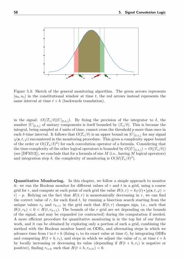
58 5. Signal Convolution Logic
u0 u0 u1 u1
Figure 5.3: Sketch of the general monitoring algorithm. The green arrows represents[u0, u1] in the constitutional window at time t, the red arrows instead represents thesame interval at time t+ h (backwards translation).
in the signal: O((Ts/δ)|U |[t,te]). By fixing the precision of the integrator to δ, thenumber |U |[t,te] of unitary components is itself bounded by (Ts/δ). This is because theintegral, being sampled at δ units of time, cannot cross the threshold p more than once ineach δ-time interval. It follows that O(Ts/δ) is an upper bound on |U |[t,te] for any signalχ(s, t, ϕ) encountered in the monitoring procedure. This gives a complexity upper boundof the order or O((Ts/δ)
2) for each convolution operator of a formula. Considering thatthe time-complexity of the other logical operators is bounded by O(|U |[t,te]) = O((Ts/δ))(see [DFM13]), we conclude that for a formula of sizeM (i.e., havingM logical operators)and integration step δ, the complexity of monitoring is O(M(Ts/δ)
2).
Quantitative Monitoring. In this chapter, we follow a simple approach to monitorit: we run the Boolean monitor for different values of r and t in a grid, using a coarsegrid for r, and compute at each point of such grid the value H(t, r) = kT (t)∗ [%(s, t, ϕ) >r] − p. Relying on the fact that H(t, r) is monotonically decreasing in r, we can findthe correct value of r, for each fixed t, by running a bisection search starting from theunique values rk and rk+1 in the grid such that H(t, r) changes sign, i.e., such thatH(t, rk) < 0 < H(t, rk+1). The bounds of the r grid are set depending on the boundsof the signal, and may be expanded (or contracted) during the computation if needed.A more efficient procedure for quantitative monitoring is in the top list of our futurework, and it can be obtained by exploring only a portion of such a grid, combining themethod with the Boolean monitor based on ODEs, and alternating steps in which weadvance time from t to t+h (fixing rt to its exact value at time t), by integrating ODEsand computing H(t+ h, rt), and steps in which we adjust the value of rt at time t+ hby locally increasing or decreasing its value (depending if H(t + h, rt) is negative orpositive), finding rt+h such that H(t+ h, rt+h) = 0.
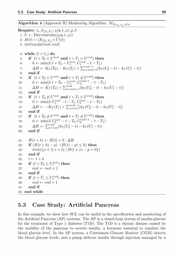
5.3. Case Study: Artificial Pancreas 59
Algorithm 4 (Approach II) Monitoring Algorithm: M〈k[T0,T1],p〉ϕ
Require: te, k[T0,T1], χ(s, t, ϕ), p, δ1: U ← Decompose(χ(s, t, ϕ))2: H(t) = (K[T0,T1] ∗ U)(t)3: initialize(init, end)
4: while (t < te) do5: if (t+ T0 ∈ U init and t+ T1 ∈ Uend) then6: h← min(δ, t+ T0 − U init1 , Uend1 − t− T1)
7: ∆H ← KT (T0)−KT (T1) +∑end−1i=init+1(kT (U i0 − t)− kT (U i1 − t))
8: end if9: if (t+ T0 ∈ U init and t+ T1 6∈ Uend) then
10: h← min(δ, t+ T0 − U init1 , Uend+10 − t− T1)
11: ∆H ← KT (T0) +∑endi=init+1(kT (U i0 − t)− kT (U i1 − t))
12: end if13: if (t+ T0 6∈ U init and t+ T1 ∈ Uend) then14: h← min(δ, Uend1 − t− T1, U
init0 − t− T0)
15: ∆H ← −KT (T1) +∑end−1i=init(kT (U i0 − t)− kT (U i1 − t))
16: end if17: if (t+ T0 6∈ U init and t+ T1 6∈ Uend) then18: h← min(δ, U init0 − t− T0, U
end+10 − t− T1)
19: ∆H ←∑endi=init(kT (U i0 − t)− kT (U i1 − t))
20: end if
21: H(t+ h)← H(t) + h ·∆H22: if (H(t+ h)− p) · (H(t)− p) ≤ 0) then23: find(x ∈ [t, t+ h] | H(t+ x)− p = 0)24: end if25: t← t+ h26: if (t+ T0 ≥ U init1 ) then27: init← init+ 128: end if29: if (t+ T1 ≤ Uend1 ) then30: end← end+ 131: end if32: end while
5.3 Case Study: Artificial Pancreas
In this example, we show how SCL can be useful in the specification and monitoring ofthe Artificial Pancreas (AP) systems. The AP is a closed-loop system of insulin-glucosefor the treatment of Type 1 diabetes (T1D). The T1D is a chronic disease caused bythe inability of the pancreas to secrete insulin, a hormone essential to regulate theblood glucose level. In the AP system, a Continuous Glucose Monitor (CGM) detectsthe blood glucose levels, and a pump delivers insulin through injection managed by a
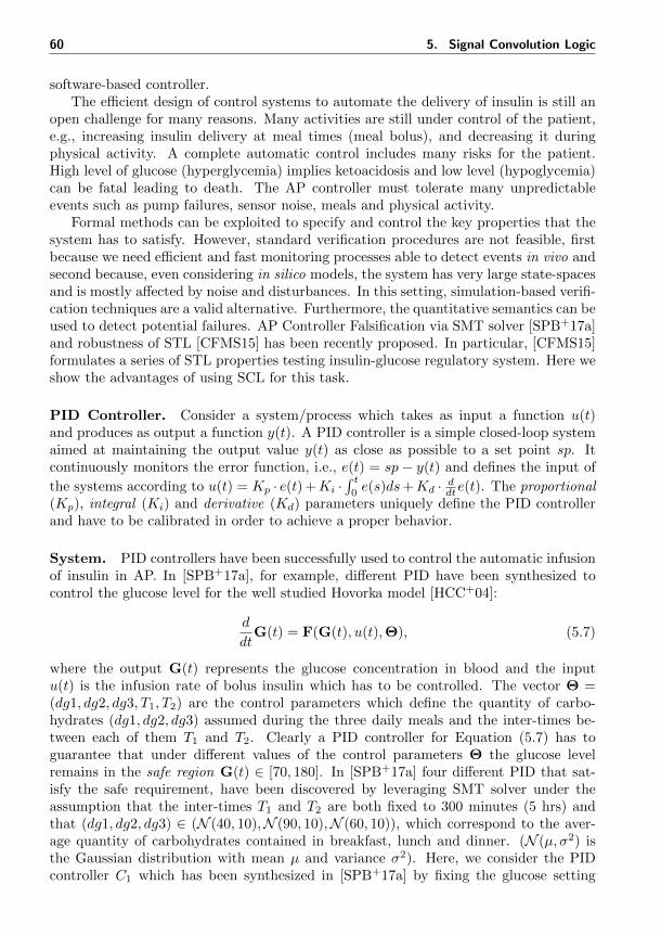
60 5. Signal Convolution Logic
software-based controller.The efficient design of control systems to automate the delivery of insulin is still an
open challenge for many reasons. Many activities are still under control of the patient,e.g., increasing insulin delivery at meal times (meal bolus), and decreasing it duringphysical activity. A complete automatic control includes many risks for the patient.High level of glucose (hyperglycemia) implies ketoacidosis and low level (hypoglycemia)can be fatal leading to death. The AP controller must tolerate many unpredictableevents such as pump failures, sensor noise, meals and physical activity.
Formal methods can be exploited to specify and control the key properties that thesystem has to satisfy. However, standard verification procedures are not feasible, firstbecause we need efficient and fast monitoring processes able to detect events in vivo andsecond because, even considering in silico models, the system has very large state-spacesand is mostly affected by noise and disturbances. In this setting, simulation-based verifi-cation techniques are a valid alternative. Furthermore, the quantitative semantics can beused to detect potential failures. AP Controller Falsification via SMT solver [SPB+17a]and robustness of STL [CFMS15] has been recently proposed. In particular, [CFMS15]formulates a series of STL properties testing insulin-glucose regulatory system. Here weshow the advantages of using SCL for this task.
PID Controller. Consider a system/process which takes as input a function u(t)and produces as output a function y(t). A PID controller is a simple closed-loop systemaimed at maintaining the output value y(t) as close as possible to a set point sp. Itcontinuously monitors the error function, i.e., e(t) = sp− y(t) and defines the input of
the systems according to u(t) = Kp · e(t) +Ki ·∫ t
0e(s)ds+Kd · ddte(t). The proportional
(Kp), integral (Ki) and derivative (Kd) parameters uniquely define the PID controllerand have to be calibrated in order to achieve a proper behavior.
System. PID controllers have been successfully used to control the automatic infusionof insulin in AP. In [SPB+17a], for example, different PID have been synthesized tocontrol the glucose level for the well studied Hovorka model [HCC+04]:
d
dtG(t) = F(G(t), u(t),Θ), (5.7)
where the output G(t) represents the glucose concentration in blood and the inputu(t) is the infusion rate of bolus insulin which has to be controlled. The vector Θ =(dg1, dg2, dg3, T1, T2) are the control parameters which define the quantity of carbo-hydrates (dg1, dg2, dg3) assumed during the three daily meals and the inter-times be-tween each of them T1 and T2. Clearly a PID controller for Equation (5.7) has toguarantee that under different values of the control parameters Θ the glucose levelremains in the safe region G(t) ∈ [70, 180]. In [SPB+17a] four different PID that sat-isfy the safe requirement, have been discovered by leveraging SMT solver under theassumption that the inter-times T1 and T2 are both fixed to 300 minutes (5 hrs) andthat (dg1, dg2, dg3) ∈ (N (40, 10),N (90, 10),N (60, 10)), which correspond to the aver-age quantity of carbohydrates contained in breakfast, lunch and dinner. (N (µ, σ2) isthe Gaussian distribution with mean µ and variance σ2). Here, we consider the PIDcontroller C1 which has been synthesized in [SPB+17a] by fixing the glucose setting

5.3. Case Study: Artificial Pancreas 61
point sp to 110mg/dl and maximizing the probability to remain in the safe region, pro-vided a distribution of the control parameter Θ as explained before. We consider nowsome properties which can be useful to check expected or anomalous behaviors of anAP controller.
Hypoglycemia and Hyperglycemia. Consider the following informal specifications:never during the day the level of glucose goes under 70mg/dl, and never during theday the level of glucose goes above 180mg/dl, which technically mean that the pa-tient is never under Hypoglycemia or hyperglycemia, respectively. These behaviors canbe formalized with the two STL formulas ϕHOSTL = G[0,24h]G(t) ≥ 70 and ψHRSTL =G[0,24h]G(t) ≤ 180. The problem of STL is that it does not distinguish if these twoconditions are violated for a second, few minutes or even hours. It only says thoseevents happen. Here we propose stricter requirements described by the two followingSCL formulas ϕHOSCL = 〈flat[0,24h], 0.95〉G(t) ≥ 70 for the Hypoglycemia regime, andϕHRSCL = 〈flat[0,24h], 0.95〉G(t) ≤ 180 for the hyperglycemia regime. We are imposingnot that globally in a day the hypoglycemia and the hyperglycemia event never occur,but that these conditions persist for at least 95% of the day (i.e., 110 minutes). We willshow above in a small test case how this requirement can be useful.
Prolongated Conditions. As already mentioned in the motivating example, themost dangerous conditions arise when hypoglycemia or hyperglycemia last for a pro-longated period of the day. In this context a typical condition is the Prolongated Hy-perglycemia which happens if the total time under hyperglycemia (i.e., G(t) ≥ 180)exceed the 70% of the day, or the Prolongated Severe Hyperglycemia when thelevel of glucose is above 300mg/dl for at least 3 hrs in a day. The importance of thesetwo conditions has been explained in [SKC+17], however the authors cannot formal-ized them in STL. On the contrary, SCL is perfectly suited to describe these conditionsas shown by the following two formulas: ϕPHRSCL = 〈flat[0,24h], 0.7〉G(t) ≥ 180 andϕPSHRSCL = 〈flat[0,24h], 0.125〉G(t) ≥ 300. Here we use flat kernels to mean that the pe-riod of a day where the patient is under Hyperglycemia or Severe Hyperglycemia doesnot count to the evaluation of the Boolean semantics. Clearly, a hyperglycemia regimein different times of the day can count differently. In order to capture this “preference”we can use non-constant kernels.
Correctness of the insulin delivery. During the hypoglycemia regime the insulinshould not be provided. The SCL formula: G[0,24h](〈flat[0,10min], 0.95〉G(t) ≤ 70 →〈flat[0,10min], 0.90〉 I(t) ≤ 0) states that if during the next 10 minutes the patient is inhypoglycemia for at least the 95% of the time then the delivering insulin pump is shut off(i.e., I(t) ≤ 0) for at least the 90% of the time. This is the “cumulative” version of theSTL property G[0,24h](G(t) ≤ 70 → I(t) ≤ 0) which says that in hypoglycemia regimeno insulin should be delivered. During the hyperglycemia regime the insulin shouldbe provided as soon as possible. The property SCL formula: G[0,24h](G(t) ≥ 300 →〈exp[−1][0,10min], 0.9〉 I(t) ≥ k) says that if we are in severe hyperglycemia regime (i.e.,G(t) ≥ 300) the delivered insulin should be higher than k for at least the 90% of thefollowing 10 minutes. We use a negative exponential kernel to express (at the robustnesslevel) the preference of having a higher value of delivered insulin as soon as possible.

62 5. Signal Convolution Logic
Figure 5.4: (left),(middle) The solution of the SCL formula falsification (red line)maximize the time under hypoglycemia (left) and hyperglycemia (right), whereas thesolution of the STL formula falsification (blue line) maximizes the displacement w.r.tthe predicate thresholds. (right) Solution of the falsification for the SCL propertiesϕPHRSCL (blue line) and ϕPHRSCL(Gauss) (red line) which implement flat and gauss kernel,respectively.
Test Case: falsification. As a first example we show how SCL logic can be effec-tively used for falsification. The AP control system has to guarantee that the level ofglucose remains in a safe region, as explained before. The falsification approach con-sists in identifying the control parameters (Θ∗) which force the system to violate therequirements, i.e., to escape from the safe region. The standard approach consists inminimizing the robustness of suited temporal logic formulas which express the afore-mentioned requirements, e.g. ϕHRSCL, ϕ
HOSCL. In this case the minimization of the STL
robustness forces the identification of the control parameters which causes the genera-tion of trajectories with a maximum displacement under the threshold 70 or above 180.To show differences among the STL and SCL logics, we consider the PID C1 + Hov-orka model and perform a random sampling exploration among its input parameters.At each sampling we calculate the robustness of the STL formulas ϕHOSTL and the SCLformula ϕHOSCL and separately store the minimum robustness value. For this minimumvalue, we estimate the maximum displacement with respect to the hypoglycemia andhyperglycemia thresholds and the maximum time spent violating the hypoglycemia andhyperglycemia thresholds. Fig. 5.4(left, middle) shows the trajectory with minimumrobustness. We can see that the trajectory which minimizes the robustness of the STLformula has a higher value of the displacement from the hypoglycemia (13) and hyper-glycemia (98) thresholds than SCL trajectory (which are 11 and 49 respectively). Onthe contrary, the trajectory which minimizes the robustness of the SCL formula remainsunder hypoglycemia (for 309 min) and hyperglycemia (for 171 min) longer than the STLtrajectory (189 min and 118 min, respectively). These results show how the convolu-tional operator and its quantitative semantics can be useful in a falsification procedure.This is particularly evident in the Hyperglycemia case (Fig. 5.4 (middle) ) where thefalsification of the SCL hyperglycemia formula ϕHRSCL shows two subintervals where thelevel of glucose is above the threshold. In order to show the effect of non-homogeneouskernel, we perform the previous experiment, with the same setting, for properties ϕPHRSCL
and ϕPHRSCL(Gauss). From the results (Fig. 5.4 (right)) is evident how the Gaussian kernel
of property ϕPHRSCL(Gauss) forces the glucose to be higher of the hyperglycemia threshold

5.4. Conclusion and Future Works 63
noise free with noiseh55 h60 h65 h70 h55 h60 h65 h70
F[0, 24h] 0.00 0.19 0.81 1.00 0.98 1.00 1.00 1.00〈flat[0,24], 0.03〉 0.00 0.00 0.20 0.91 0.00 0.02 0.77 1.00
Table 5.2: Results of the falsification test case. The performance of STL and SCLformulas verified on the PID C1 + Hovorka model with noise and noise free are compared.The STL formula on the noisy model is uninformative.
just before the first meal (t ∈ [0, 200]) and ignores for example the last meal (t ≥ 600).
Test Case: noise robustness. Now we compare the sensitivity to noise of SCLand STL formulae. We consider three degrees of hypoglycemia hk(t) = G ≤ k,where k ∈ 55, 60, 65, 70 and estimate the probability that the Hovorka model con-trolled by the usual PID C1 (i.e., PID C1 + Hovorka Model) satisfies the STL formulasϕkSTL = F[0, 24h]hk and the SCL formulas ϕkSCL = 〈flat[0,24h], 0.03〉hk under the usualdistribution assumption for the control parameters Θ. The results are reported in col-umn “noise free” of Table 5.2. Afterwards, we consider a noisy outcome of the samemodel by adding a Gaussian noise, i.e., ε ∈ N (0, 5), to the generated glucose trajectory.We estimate the probability that this noisy system satisfies the STL and SCL formulasabove, see column “with noise” of Table 5.2. The noise corresponds to the disturbanceof the original signals which can occur, for example, during the measurement process.
As shown in Table 5.2, the probability estimation of the STL formulas changesdrastically with the addition of noise (the addition of noise forces all the trajectory tosatisfy the STL formula). On the contrary, the SCL formulas ϕkSCL are more stableunder noise and can be even used to approximate the probability of the STL formulason the noise-free model. To better asses this, we checked how much the STL formulaϕkSTL and the SCL formula ϕkSCL, evaluated in the noisy model, agree with the STLformula ϕkSTL evaluated in the noise-free model, by computing their truth value on 2000samples, each time choosing a random threshold k ∈ [50, 80]. The score for STL is 56%,while SCL agrees on 78% of the cases.
5.4 Conclusion and Future Works
We have introduced SCL, a novel specification language that employs signal processingoperations to reason about temporal behavioural patterns. The key idea is the definitionof a family of modal operators which compute the convolution of a kernel with the signaland check the obtained value against a threshold. Our case study on monitoring glu-cose level in artificial pancreas demonstrates how SCL empowers the classical temporallogic operators (i.e., such as finally and globally) with noise filtering capabilities, andenable us to express temporal properties with soft time bounds and with nonsymmetrictreatment of time instants in a unified way. The convolution operator of SCL can beseen as a syntactic bridge between temporal logic and digital signal processing, tryingto combine the advantages of both these two worlds. This point of view can be exploredfurther, bringing into the monitoring algorithms of SCL tools from frequency analysis

64 5. Signal Convolution Logic
of signals. Future work includes the release of a Python library and the design of effi-cient monitoring algorithms also for the quantitative semantics. Finally, we also planto develop online monitoring algorithms for real-time systems using hardware dedicatedarchitecture such as field-programmable gate array (FPGA) and digital signal processor(DSP).


66 5. Signal Convolution Logic

6Classification of Trajectories
Learning temporal logic requirements from temporal data is an emergent research fieldgaining momentum in the rigorous engineering of cyber-physical systems. Classical ma-chine learning methods typically generate very powerful black box (statistical) models.However, these models often do not help in the comprehension of the phenomenon theycapture. Temporal logic provides a precise formal specification language that can beeasily interpreted by humans. The possibility to describe data sets in a concise wayusing temporal logic formulae can thus help to better clarify and comprehend whichare the emergent patterns for the system at hand. A clearcut example is the prob-lem of anomaly detection, where the input is a set of trajectories describing regular oranomalous behaviors, and the goal is to learn a classifier that not only can be used todetect anomalous behaviors at runtime, but also gives insights on what characterizesan anomalous behavior. Learning temporal properties is also relevant in combinationwith state of the art techniques for search-based falsification of complex closed-loopsystems [ZSD+15, SKC+17, BBNS15, SPB17b], as it can provide an automatic way todescribe unwanted (or desired) behaviors that the system needs to satisfy.
In this contribution, we consider the problem of learning a temporal logic specifica-tion from a set of trajectories which are labeled either as good for the normally expectedbehaviors or as bad for the anomalous ones. The goal is to automatically synthesize boththe structure of the formula and its parameters providing a temporal logic classifier thatcan discriminate as much as possible the bad and the good behaviors. This specificationcan be turned into a monitor that outputs a positive verdict for good behaviors and anegative verdict for bad ones.
Related Work. Mining temporal logic requirements is an emerging field of research inthe analysis of cyber-physical systems [ADMN11, YHF12, BBS14a, JDDS15, NKJ+17,ZRWT17, KJB17, BVP+16, BBS+14b].
This approach is orthogonal to Active Automata Learning (AAL) such as L∗ An-gluin’s algorithm [Ang87] and its recent variants [IHS14, SHI12]. AAL is suitable tocapture the behaviours of black box reactive systems and it has been successfully em-ployed in the field of Cyber-physical Systems (CPS) to learn how to interact with the
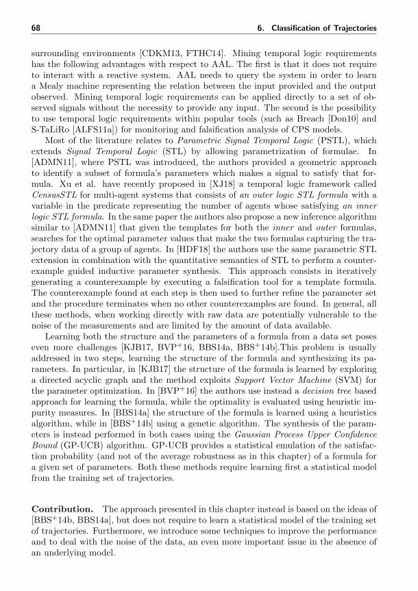
68 6. Classification of Trajectories
surrounding environments [CDKM13, FTHC14]. Mining temporal logic requirementshas the following advantages with respect to AAL. The first is that it does not requireto interact with a reactive system. AAL needs to query the system in order to learna Mealy machine representing the relation between the input provided and the outputobserved. Mining temporal logic requirements can be applied directly to a set of ob-served signals without the necessity to provide any input. The second is the possibilityto use temporal logic requirements within popular tools (such as Breach [Don10] andS-TaLiRo [ALFS11a]) for monitoring and falsification analysis of CPS models.
Most of the literature relates to Parametric Signal Temporal Logic (PSTL), whichextends Signal Temporal Logic (STL) by allowing parametrization of formulae. In[ADMN11], where PSTL was introduced, the authors provided a geometric approachto identify a subset of formula’s parameters which makes a signal to satisfy that for-mula. Xu et al. have recently proposed in [XJ18] a temporal logic framework calledCensusSTL for multi-agent systems that consists of an outer logic STL formula with avariable in the predicate representing the number of agents whose satisfying an innerlogic STL formula. In the same paper the authors also propose a new inference algorithmsimilar to [ADMN11] that given the templates for both the inner and outer formulas,searches for the optimal parameter values that make the two formulas capturing the tra-jectory data of a group of agents. In [HDF18] the authors use the same parametric STLextension in combination with the quantitative semantics of STL to perform a counter-example guided inductive parameter synthesis. This approach consists in iterativelygenerating a counterexample by executing a falsification tool for a template formula.The counterexample found at each step is then used to further refine the parameter setand the procedure terminates when no other counterexamples are found. In general, allthese methods, when working directly with raw data are potentially vulnerable to thenoise of the measurements and are limited by the amount of data available.
Learning both the structure and the parameters of a formula from a data set poseseven more challenges [KJB17, BVP+16, BBS14a, BBS+14b].This problem is usuallyaddressed in two steps, learning the structure of the formula and synthesizing its pa-rameters. In particular, in [KJB17] the structure of the formula is learned by exploringa directed acyclic graph and the method exploits Support Vector Machine (SVM) forthe parameter optimization. In [BVP+16] the authors use instead a decision tree basedapproach for learning the formula, while the optimality is evaluated using heuristic im-purity measures. In [BBS14a] the structure of the formula is learned using a heuristicsalgorithm, while in [BBS+14b] using a genetic algorithm. The synthesis of the param-eters is instead performed in both cases using the Gaussian Process Upper ConfidenceBound (GP-UCB) algorithm. GP-UCB provides a statistical emulation of the satisfac-tion probability (and not of the average robustness as in this chapter) of a formula fora given set of parameters. Both these methods require learning first a statistical modelfrom the training set of trajectories.
Contribution. The approach presented in this chapter instead is based on the ideas of[BBS+14b, BBS14a], but does not require to learn a statistical model of the training setof trajectories. Furthermore, we introduce some techniques to improve the performanceand to deal with the noise of the data, an even more important issue in the absence ofan underlying model.

6.1. Problem Formulation 69
First, instead of using the probability satisfaction as an evaluator for the best for-mula, we consider the average robustness (Section 2.5) which enables us to differentiateamong STL classifiers that have similar classification performance with respect to thedata by choosing the most robust one. This gives us more information than just havingthe probability of satisfaction: for each trajectory, we can evaluate how much is it closeto the “boundary” of the classifier, instead of only checking whether it satisfies or not aformula. We then modify the discrimination function and the GP-UCB algorithm (Sub-section 4.1.1) used in [BBS14a] and [BBS+14b] to better deal with the noise of the dataand to use the quantitative semantics to emulate the average robustness distributionwith respect to the parameter space of the formula.
Second, we reduce the computational cost of the Evolutionary Algorithm (EA) (im-plemented in [BBS+14b]), by using a lightweight configuration (i.e., a low threshold ofthe max number of iterations) of the GP-UCB optimization algorithm to estimate theparameters of the formulae at each generation. The EA algorithm generates, as a finalresult, an STL formula tailored for classification purpose.
Finally, we compare our framework with the methodology of [BBS+14b] and withthe decision-tree based approach presented in [BVP+16] on an anomalous trajectorydetection problem of naval surveillance.
6.1 Problem Formulation
Let us start with the definition of the parametric signal temporal logic which we use inthe rest of this chapter.
PSTL Parametric Signal Temporal Logic [ADMN11] is an extension of STL thatparametrizes the formulae. There are two types of formula parameters: temporal param-eters, corresponding to the time bounds in the time intervals associated with temporaloperators (e.g., a, b ∈ R+
0 , with a < b, s.t. F[a,b]µ) and the threshold parameters corre-sponding to the constants in the inequality predicates (e.g., k ∈ R, µ = xi > k, wherexi is a variable of the trajectory). In this work, we allow only atomic propositions ofthe form µ = xi ./ k with ./∈ >,≤. Given an STL formula ϕ, let K = (T × C)be the parameter space, where T ⊆ (R+
0 )nt is the temporal parameter space (nt beingthe number of temporal parameters), and C ⊆ Rnk is the threshold parameter space(nk being the number of threshold parameters). A ϑ ∈ K is a parameter configurationthat induces a corresponding STL formula; e.g., ϕ = F[a,b](xi > k),ϑ = (0, 2, 3.5) thenϕϑ = F[0,2](xi > 3.5).
We focus our attention on learning the best property (or set of properties) thatdiscriminates trajectories belonging to two different classes, say good and bad, start-ing from a labeled data set of observed trajectories. Essentially, we want to tackle asupervised two-class classification problem over paths, by learning a temporal logic dis-criminant, describing the temporal patterns that better separate two sets of observedpaths.
The idea behind this approach is that there exists an unknown procedure that, givena temporal trajectory, is able to decide if the signal is good or bad. This procedure cancorrespond to many different things, e.g., to the reason of failure of a sensor that breaks

70 6. Classification of Trajectories
when it receives specific inputs. Our task is to approximate this unknown procedurewith an STL monitoring algorithm. In general, as there may not be an STL formula thatperfectly explains/mimics the unknown process, our task is to find the most effectiveone.
The approach we present here works directly with observed data and avoids thereconstruction of an intermediate generative model p(x|c) of trajectories x conditionedon their class c, as in [BBS+14b, BBS14a]. The reason is that such models can behard to construct, even if they provide a powerful regularization, as they enable thegeneration of an arbitrary number of samples to train the logic classifier.
In a purely data-driven setting, to build an effective classifier, we need to deal withthe fact that training data is available in limited amounts and it is typically noisy. Thisreflects the necessity of finding methods that guarantee good generalization performanceand avoid overfitting. In our context, overfitting can result in overly complex formulae,de facto encoding the training set itself rather than guessing the underlying patternsthat separate the trajectories. This can be faced by using a score function based on therobustness of temporal properties, combined with suitably designed regularizing terms.
We want to stress that the approach we present here, due to the use of the av-erage robustness of STL properties, can be easily tailored to different problems, likeapprenticeship learning, i.e., finding the property that best characterizes a single set ofobservations.
6.2 Methodology
Learning an STL formula can be separated into two optimization problems: the learningof the formula structure and the synthesis of the formula parameters. The structurallearning is treated as a discrete optimization problem using Genetic Algorithm (GA);the parameter synthesis, instead, considers a continuous parameter space and exploitsan active learning algorithm called Gaussian Process Upper Confidence Bound (GP-UCB) algorithm. The two techniques are not used separately but combined together ina bi-level optimization. The GA act externally by defining a set of template formulae.Then, the GP-UCB algorithm, which acts at the inner level, finds the best parameterconfiguration such that each template formula better discriminates between the two datasets. To apply this second optimization we need to define a score function to optimize,encoding the criterion to discriminate between the two data sets.
Our implementation, called RObustness GEnetic (ROGE) algorithm is describedin Algorithm 5. First, we give an overview of it and then we described each specificfunction in the next subsections. The algorithm requires as input the data set Dp(good)and Dn(bad), the parameter space K, with the bounds of each formula parameters,the size of the initial set of formulae Ne, the number of iterations Ng, the mutationprobability α and the initial formula size s.
line 1) It starts generating an initial set of PSTL formulae, called gen.
line 2) For each of these formulae, the algorithm learns the best parameters accordinglyto a discrimination function G. We call genΘ the generation for which we knowthe best parameters of each formula.

6.2. Methodology 71
line 3) The algorithm starts the iterations.
line 4) The algorithm, guided by a fitness function F, extracts a subset subgΘ composedby the best Ne/2 formulae, from the initial set genΘ. The formulae are extractedproportionally to their fitness values (e.g., a formula with a double F-value w.r.tto another one, has a doubled probability to be sampled).
line 5) From this subset, a new set newg composed of Ne formulae is created by em-ploying the Evolve routine, which implements two genetic operators.
line 6) As in line 2, the algorithm identifies the best parameters of each formula be-longing to newg.
line 7) The new generation newgΘ and the old generation genΘ are then merged to-gether. From this set of 2Ne formulae the algorithm extracts, with respect to thefitness function F , the new generation genΘ of Ne formulae.
line 9) At the end of the iterations, the algorithm returns the last generated formulae.The best formula is the one with the highest value of the discrimination function,i.e., ϕbest = argmaxϕϑ∈genΘ
(G(ϕϑ)).
We describe below in order: the discrimination function, the learning of the formulaparameters and the learning of the formula structure.
6.2.1 Discrimination Function
We have two data sets Dp and Dn and we search for the formula ϕ that better separatesthese two classes. We define a function able to discriminate between this two datasets, such that maximizing this discrimination function corresponds to finding the bestformula classifier. We decide to use, as evaluation of satisfaction of each formula, thequantitative semantics of STL. As described in Subsection 2.1.1, this semantics returnsa real-value of satisfaction instead of only a yes/no answer.
Given a data set Di, we assume that the data comes from an unknown stochasticprocess M. The process, in this case, is like a black box for which we observe only asubset of trajectories, the data set Di. We can then evaluate the averages robustnessE(Rϕ|M) and its variance σ2(Rϕ|M), averaging over Di, (see Section 2.5).
To discriminate between the two data sets Dp and Dn, we search the formula ϕ thatmaximizes the difference between the average robustness of Mp, E(Rϕ|Mp), and theaverage robustness of Mn, E(Rϕ|Mn) divided by the sum of the respective standarddeviation.
G(ϕ) =E(Rϕ|Mp)− E(Rϕ|Mn)
σ(Rϕ|Mp) + σ(Rϕ|Mn)(6.1)
This formula is proportional to the probability that a new point sampled from the samedistribution of points generatingMp orMn, will belong to one set and not to the other.In fact, an higher value of G(ϕ) implies that the two average robustness scores will besufficiently far away, compared to their length-scale, given by the standard deviation σ.
As said above, we can evaluate just a statistical approximation of G(ϕ) because weare working with just evaluations of the unknown functions E(Rϕ|M). We will see inthe next paragraph how we tackle this problem.

72 6. Classification of Trajectories
6.2.2 GP-UCB: learning the parameters of the formula
Given a formula ϕ and a parameter space K, we want to find the parameter configurationϑ ∈ K that maximises the score function g(ϑ) := G(ϕϑ), considering that we have onlynoise and costly evaluation of it. The question is therefore how to best estimate (andoptimize) an unknown function from observations of its value at a finite set of inputpoints. This is a classic non-linear non-convex optimization problem that we tackle bymeans of the GP-UCB algorithm (Subsection 4.1.1). This algorithm interpolates thenoisy observations using a stochastic process (a procedure called emulation in statistics)and optimize the emulation function using the uncertainty of the fit to determine regionswhere the true maximum can lie. More specifically, the GP-UCB bases its emulationphase on Gaussian Processes (GP), a Bayesian non-parametric regression approach,adding candidate maximum points to the training set of the GP in an iterative fashion,and terminating when no improvement is possible (see Section 4.1 and [SKKS12] formore details). After this optimization, we have found a formula that separates the twodata sets, not from the point of view of the satisfaction (yes/no) of the formula butfrom the point of view of the robustness value. In other words, there is a thresholdvalue α such that E(Rϕ|Mp) > α and E(Rϕ|Mn) ≤ α. Now, we consider the newSTL formula ϕ′ obtained translating the atomic predicates of ϕ by α (e.g., y(x) > 0becomes y(x)−α > 0). Taking into account that the quantitative robustness is achievedby combination of min, max, inf and sup, which are linear algebraic operators w.r.ttranslations (e.g, min(x, y)±c = min(x±c, y±c)), we easily obtain that E(Rϕ′ |Mp) > 0and E(Rϕ′ |Mn) < 0. Therefore, considering the soundness of the robustness semanticsof STL, we have that ϕ′ divides the two data set also from the point of view of thesatisfaction.
We remark that the use of the robustness degree of STL hampers to use the minimalrepresentation of the formula. Indeed, even if the minimal representation has the sameBoolean satisfaction it can have different robustness values.
6.2.3 Genetic Algorithm: learning the structure of the formula
To learn the formula structure, we exploit a modified version of the Genetic Algorithm(GA) presented in [BBS+14b]. In Section 4.2 we provide an overview of this approach.Genetic Algorithms belong to the larger class of evolutionary algorithms (EA). Theyare used for search and optimization problems. The strategy takes inspiration from thegenetic area, in particular in the selection strategy of species. Let us see now in detailthe genetic routines of the ROGE algorithm.
gen = generateInitialFormulae(Ne, s). This routine generates the initial set ofNe formulae. A fraction nl < Ne of this initial set is constructed by a subset ofthe temporal properties: FIµ, GIµ, µ1UIµ2, where the atomic predicates are of theform µ = (xi > k) or µ = (xi ≤ k) or simple Boolean combinations of them (e.g.,µ = (xi > ki)∧ (xj > kj)). The size of this initial set is exponential w.r.t the number ofconsidered variables xi. If we have few variables we can keep all the generated formulae,whereas if the number of variables is large we consider only a random subset. Theremain nr = Ne − nl formulae are chosen randomly from the set of formulae with amaximum size defined by the input parameter s. This size can be adapted to have a
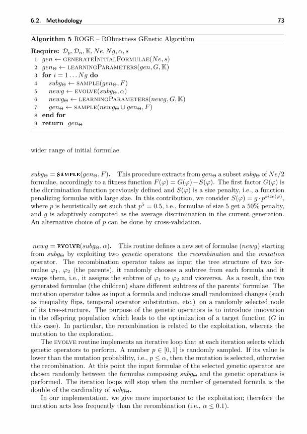
6.2. Methodology 73
Algorithm 5 ROGE – RObustness GEnetic Algorithm
Require: Dp,Dn,K, Ne,Ng, α, s1: gen← generateInitialFormulae(Ne, s)2: genΘ ← learningParameters(gen,G,K)3: for i = 1 . . . Ng do4: subgΘ ← sample(genΘ, F )5: newg ← evolve(subgΘ, α)6: newgΘ ← learningParameters(newg,G,K)7: genΘ ← sample(newgΘ ∪ genΘ, F )8: end for9: return genΘ
wider range of initial formulae.
subgΘ = sample(genΘ, F ). This procedure extracts from genΘ a subset subgΘ ofNe/2formulae, accordingly to a fitness function F (ϕ) = G(ϕ)−S(ϕ). The first factor G(ϕ) isthe dicrimination function previously defined and S(ϕ) is a size penalty, i.e., a functionpenalizing formulae with large size. In this contribution, we consider S(ϕ) = g ·psize(ϕ),where p is heuristically set such that p5 = 0.5, i.e., formulae of size 5 get a 50% penalty,and g is adaptively computed as the average discrimination in the current generation.An alternative choice of p can be done by cross-validation.
newg = evolve(subgΘ, α). This routine defines a new set of formulae (newg) startingfrom subgΘ by exploiting two genetic operators: the recombination and the mutationoperator. The recombination operator takes as input the tree structure of two for-mulae ϕ1, ϕ2 (the parents), it randomly chooses a subtree from each formula and itswaps them, i.e., it assigns the subtree of ϕ1 to ϕ2 and viceversa. As a result, the twogenerated formulae (the children) share different subtrees of the parents’ formulae. Themutation operator takes as input a formula and induces small randomized changes (suchas inequality flips, temporal operator substitution, etc.) on a randomly selected nodeof its tree-structure. The purpose of the genetic operators is to introduce innovationin the offspring population which leads to the optimization of a target function (G inthis case). In particular, the recombination is related to the exploitation, whereas themutation to the exploration.
The evolve routine implements an iterative loop that at each iteration selects whichgenetic operators to perform. A number p ∈ [0, 1] is randomly sampled. If its value islower than the mutation probability, i.e., p ≤ α, then the mutation is selected, otherwisethe recombination. At this point the input formulae of the selected genetic operator arechosen randomly between the formulas composing subgΘ and the genetic operations isperformed. The iteration loops will stop when the number of generated formula is thedouble of the cardinality of subgΘ.
In our implementation, we give more importance to the exploitation; therefore themutation acts less frequently than the recombination (i.e., α ≤ 0.1).

74 6. Classification of Trajectories
6.2.4 Regularization
In the evolutionary algorithm, we use two strategies to penalize complex formulae andbias the algorithm towards simple ones. The first strategy is to use a size penaltyS(ϕ) in the fitness function: F (ϕ) = G(ϕ) − S(ϕ). In this work, we consider S(ϕ) =g · psize(ϕ), where p is heuristically set such that p5 = 0.5, i.e., formulae of size 5 get a50% penalty, and g is adaptively computed as the average discrimination in the currentgeneration. An alternative choice of p can be done by cross-validation. The secondstrategy, instead, consists in selecting the initial population biasing it towards simpleformulae. In particular, this set is constructed by (a) a subset of random formulae and(b) a subset of logically non-equivalent temporal properties of size 1, of the form FIµ,GIµ, µ1UIµ2, where the atomic predicates µ are sampled from the subset of all atomicpredicates (with threshold zero) or simple Boolean combinations of them.
6.3 Case Study: Maritime Surveillance
We consider the maritime surveillance case study presented in [BVP+16] to compare ourframework with their Decision Tree (DTL4STL) approach. The experiments with theDTL4STL approach were implemented in Matlab with the code available at [DTL16].We also test the implementation presented in [BBS+14b] with the same benchmark.Both the new an the previous learning procedure were implemented in JAVA (JDK1.8 0) and run on a Dell XPS, Windows 10 Pro, Intel Core i7-7700HQ 2.8 GHz, 8GB1600 MHz memory.
The synthetic data set of naval surveillance reported in [BVP+16] consists of 2-dimensional coordinates traces of vessels behaviors. It considers two kinds of anomaloustrajectories and regular trajectories, as illustrated in Figure 6.1. The data set contains2000 total trajectories (1000 normal and 1000 anomalous) with 61 sample points pertrace. We fixed the training set as the 80% of the entire data set and the validation setas the rest 20% of the traces.
0 10 20 30 40 50 60 70
x1
15
20
25
30
35
40
45
x 2
Figure 6.1: The regular trajectories are represented in green. The anomalous trajectorieswhich are of two kinds, are represented respectively in blue and red.

6.3. Case Study: Maritime Surveillance 75
ROGE DTL4STL DTL4STLpMis. Rate 0 0.01± 0.01 0.007± 0.008
Comp. Time 73± 18 144± 24 -
Table 6.1: The comparison of the computational time (in seconds), the mean miss-classification rate and its standard deviation between the learning procedure using theRObust GEnetic algorithm, the Decision-Tree (DTL4STL) Matlab code provided by theauthors and the results reported in [BVP+16] (DTL4STLp).
We run the experiments using a 10-fold cross-validation to collect the mean and vari-ance of the misclassified trajectories of the validation set. The implementation presentedin [BBS+14b] performs so poorly on the chosen benchmark that is not meaningful toreport it: the misclassification rate on the validation set is around 50%.
The other obtained performances are presented in Table 6.1 as well as the average andvariance of the execution time. We also report the DTL4STL performance (DTL4STLpin Table 6.1) declared in [BVP+16], but we were not be able to reproduce them in oursetting.
An example of the formula that we learn with ROGE is
ϕ = (x2 > 22.46) U[49,287] (x1 ≤ 31.65) (6.2)
DTL4STL instead does not consider the until operator in the set of primitives (see[BVP+16] for more details) and the formula found by the tool using the same data setis the following:
ψ = (((G[187,196)x1 < 19.8) ∧ (F[55.3,298)x1 > 40.8)) ∨((F[187,196)x1 > 19.8) ∧ ((G[94.9,296)x2 < 32.2) ∨
((F[94.9,296)x2 > 32.2) ∧ (((G[50.2,274)x2 > 29.6) ∧(G[125,222)x1 < 47)) ∨ ((F[50.2,274)x2 < 29.6) ∧
(G[206,233)x1 < 16.7))))))
The specific formula generated using ROGE is simpler than the formula generatedusing DTL4STL and indeed it is easier to understand it. More specifically, the formula6.2 identifies all the regular trajectories, remarkably resulting in a misclassification errorequal to zero, as reported in Table 6.1. The red anomalous trajectories falsify thepredicate x2 > 22.46 before verifying x1 ≤ 31.65, on the contrary the blue anomaloustrajectories globally satisfy x2 > 22.46 but never verify x1 ≤ 31.65 (consider that all thevessels start from the top right part of the graphic in Figure 6.1). Both these conditionsresult in the falsification of the formula 6.2, which on the contrary is satisfied by allthe regular trajectories. In Figure 6.1, we have reported the threshold x2 = 22.46 andx1 = 31.65. In terms of accuracy, our approach is comparable w.r.t. the performanceof the DTL4STL approach shown in [BVP+16]. Similarly to other EA based approach,ROGE needs to be configured in some of its parameters (such as the mutation, therecombination probability, the fitness function and the initial population) meaning that

76 6. Classification of Trajectories
a specific setting can influence its performance.
6.4 Conclusion and Future Works
We present a framework to learn a Signal Temporal Logic (STL) specification from alabeled data set of regular and anomalous trajectories that better discriminates themin two subsets. In particular, we design a RObust GEnetic algorithm (ROGE) thatcombines an evolutionary algorithm for learning of the structure of the formula and theGaussian process upper confidence bound algorithm for the synthesis of the formula pa-rameters. We compare ROGE with [BBS+14b] and the decision tree approach presentedin [BVP+16] on an anomalous trajectory detection problem of a maritime surveillancesystem.
With respect to the previous work [BBS14a, BBS+14b], we avoid the reconstructionof a generative statistical model for the data set and present a procedure that workswell also directly with the data set. Furthermore, to improve the quality of the learn-ing procedure, we modify both the structure and the parameters of the optimizationalgorithms. Concerning the learning of the structure, we modify the evolutionary al-gorithm drastically improving its performance, in particular, we change the policy tochoose the initial formula generation and we simplify the genetic operators of muta-tion and recombination. Concerning the learning of the parameters, we leverage theaverage robustness (using the STL quantitative semantics) to discriminate also betweentwo trajectories satisfying the same STL specification, but with two distinct robustnessvalues that can be separated by a threshold. This provides more information that canbe exploited in the optimization process.
We observe that the application of the approach [BBS+14b] directly on the data setof the naval surveillance system considered here, performs very poorly. We compareour method also with the Decision Tree (DTL4STL) approach of [BVP+16] showingthat we have a comparable accuracy producing smaller and easier to understand STLspecifications. Furthermore, we do not restrict the class of the temporal formula to onlyeventually and globally and we do not impose only one possible temporal nesting. On theother hand, the genetic algorithm can get completely wrong results if the initial formulageneration is chosen completely randomly. Note that our choice of initial formulae is away to bias the search towards simple properties, i.e., it is a form of regularization andresembles the choice of the set of primitive in the DTL4STL approach.
As future work, we aim to improve the genetic algorithm avoiding the optimization ofsimilar formulae. We plan to exploit a Bootstrap aggregating (i.e., Bagging) techniqueto face the overfitting problem and guarantee good generalization performance. Theidea is to generate new subsets from the initial one, through a uniform sampling withreplacement, and apply the genetic algorithm to each subset. This will decrease theeffect of possible biases in the initial distribution of the data. Finally, we plan also totest our procedure in more interesting case studies, particularly in the presence of strongnoise in the data sets, where we believe our method can exhibit good results.

7Parameter Synthesis
Stochastic models are used to describe and simulate a wide range of dynamical systems,such as biological processes, chemical reactions, and networks dynamics. The most suc-cessful representations is this scenarios are Chemical Reaction Networks (CRN) (Defi-nition 4, Section 1.2), stochastic Petri nets [Haa04] and population models [BHLM13b].All these representations underline a CTMC which under reasonable hypothesis wellapproximate the modeled dynamical systems. For example, a chemical reaction canalways be represented as a CRN, but the underlying CTMC is a reliable approximationonly if the well-stirred hypothesis is verified.
A typical model checking problem consists in estimating the following probability
Pϕ(M) = PM(Sat(ϕ))
where ϕ is a formula in a suitable temporal logic and Sat(ϕ) = x ∈ ST | (x, 0) |= ϕ,as already defined in Section 2.4 . This is a typical a posteriori problem, where a modelis given, and some qualitative and/or quantitative information (described by means oflogics) are extracted. As already discuss in Section 2.4, there are two main approachesto solve this issue: analytical methods which compute multidimensional integrals andstatistical methods which simulate a model of a system many times. The former methodrelies on the assumption that the parameter values of the model are known, whereas thelatter on the availability of a computation model able to draw independent and identi-cally distributed trajectories. These are strong assumptions which are not satisfied inspecific contexts such as model-based design and system biology. In the early design-ing process, for example, not all the parameters are fixed, but only intervals (definedby means of expertise) are considered. Moreover, in system biology, many parametervalues are not even known because estimating them is highly costly or cannot be mea-sured. These two problems have different goals. The first problem, called ParametersSynthesis, tries to identify a set of model parameters such that a given property is ver-ified or a given probability maximized. On the contrary, the second problem, calledSystem Identification follows a reverse direction. It considers the satisfiability of a set ofdifferent formulae against a target systems with the aim of identifying a neighborhood
78 7. Parameter Synthesis
of the parameter model (which well approximate that target system). In this chapter,we describe a statistical approach which relies on Smoothed Model Checking (smMC)(Section 3.2) to solve the parameter synthesis problem that we define in a particularsetting.
Related work. Parameter synthesis of CTMC is an active field of research. In[CDKP14] and [CDP+17] the authors use Continuous Stochastic Logic (CSL) and uni-formization methods for computing exact probability bounds for parametric modelsof CTMCs obtained from chemical reaction networks. In [CPP+16] the same authorsextend their algorithm to GPU architecture to improve the scalability. Authors inthese two papers solve two problems: one is the threshold synthesis, the other is theidentification of a parameter configuration maximizing the satisfaction probability. Inthis chapter, we focus on the former, as we already presented a statistical approach todeal the latter problem in [BBNS15] for the single objective case and in [BPS16] forthe multi-objective case (see also Chapter 8). An alternative statistical approach formulti-objective optimization is that of [DDL+13], where authors use ANOVA test toestimate the dominance relation. Another approach to parameter synthesis for CTMCis [HKM08], where the authors rely on a combination of discretization of parameterswith a refinement technique.
In this work we use a statistical approach to approximate the satisfaction probabil-ity function, building on smoothed model checking [BMS16]. This approach applies toCTMC with rate functions that are smooth with respect to parameters and leveragesstatistical tools based on Gaussian process regression [RW06] to learn an approximationof the satisfaction function from few observations. Moreover, this approach allows us todeal with a richer class of linear time properties than reachability, like those describedby metric temporal logic [AFH96, MN04], for which numerical verification routines areheavily suffering from state space explosion [BCH+11]. Another statistical approach isthat of [JL11], which combines sensitivity analysis, statistical model checking and uni-form continuity to approximate the satisfaction probability function, but it is restrictedto cases when the satisfaction probability is monotonic in the parameters. In contrast,Gaussian process-based methods have no restriction (as Gaussian processes are univer-sal approximators), and also have the advantage of requiring much fewer simulationsthan pointwise statistical model checking, as information is shared between neighboringpoints (see [BMS16] for a discussion in this sense). Parametric verification and synthe-sis approaches are more consolidated for discrete time Markov chains [Kat16], wheremature tools like PROPhESY exist [DJJ+15], which rely on a symbolic representationof the reachability probability, which does not generalize to the continuous time setting.
Contribution. We propose a Bayesian statistical approach for parameter synthe-sis, which leverages a statistical parameterised verification method known as smoothedmodel checking [BMS16] (Section 3.2) and the nice theoretical approximation propertiesof Gaussian process [RW06] (Section 3.1). Being based on a Bayesian inference engine,this naturally gives statistical error bounds for the estimated probabilities. Our algo-rithm uses active learning strategies to steer the exploration of the parameter space onlywhere the satisfaction probability is close to the threshold. We also provide a prototypeimplementation of the approach in Python.

7.1. Problem Formulation 79
Despite being implemented in Python, our approach turns to be remarkably efficient,being slightly faster than [CDP+17] for small models, and outperforming it for morecomplex and large models or when the number of parameters is increased, at the priceof a weaker form of correctness. Compared to [CDP+17], we also have an additionaladvantage: the method treats the simulation engine and the routine to verify the lin-ear time specification on individual trajectories as black boxes. This means that, notonly, we can handle arbitrary MTL properties (while in [CDP+17] there is an essentialrestriction to non-nested CSL properties, i.e., reachability), but also other more compli-cated linear time specifications (e.g., using hybrid automata, providing the satisfactionprobability is a smooth function of model parameters). Moreover, we can also applythe same approach to more complex stochastic models for which efficient simulationroutines exist, like stochastic differential equations.
7.1 Problem Formulation
Statistical Threshold Synthesis Problem. We consider a family Mϑ of CTMCindexed by continuous parameters ϑ which assume values in a compact hyperrectangleΘ ⊂ Rk. We also assume that Mϑ depend smoothly on ϑ through their rate func-tions and consider a linear time specifications ϕ described by Metric Interval TemporalLogic [MN04], with bounded time operators. Our goal is to find the subset of parametersΓα ⊂ Θ such that Pϕ(ϑ) ≥ α for a threshold α, where Pϕ(ϑ) represents the probabil-ity that Mϑ satisfies ϕ, see Section 2.4. We introduce the positive class Pα, which iscomposed of parameter values for which the probability of satisfying ϕ is higher thana threshold value α, the negative class Nα, composed of parameters values for whichthis probability is lower than α, and the undefined class Uα, which collects all the otherparameter values. This class represents the region where it is not possible to decide ifPϕ(ϑ) ≥ α or Pϕ(ϑ) ≤ α. Following [CDP+17], we will look for a partition where thevolume of the undefined class is lower a fraction of the volume of Θ. This problem iscalled threshold synthesis problem and it was originally introduced and solved by analyt-ical technique in [CDP+17]. This contribution is based on the min max approximationwhere the idea is to consider a subset H ⊆ Θ and estimating, with a variable degree ofaccuracy, the minimum and the maximum of Pϕ(ϑ). For example if we estimate that
[minϑ∈H
Pϕ(ϑ),maxϑ∈H
Pϕ(ϑ)] ⊆ [λHmin, λHmax]
we can easily decide if H belongs to Pα or Nα just by considering if λHmin > α orλHmax < α respectively. Otherwise H is divided into two subsets H0 and H1 and thealgorithm is iterated over them. This procedure stops when the volume of Uα is belowa given threshold. The converge is assured by the sub-linearity of the min and the max.
In Section 2.4 we already discussed the drawbacks of the analytical methods. In thiscase, the same considerations apply, yet the possibility of parallelizing the algorithmmitigates them.
Our approach, on the other hand, will be statistic: we assume that models are toocomplex to numerically compute bounds on the reachability probability, and we onlyrely on the possibility of simulating the model. As a consequence, our solution to theparameter synthesis problem will have only statistical guarantees of being correct. For

80 7. Parameter Synthesis
example, if a parameter belongs to Pα, the confidence of this point satisfying Pϕ(ϑ) ≥ αwill be larger than a prescribed probability (typically 95% or 99%), though for mostpoints this probability will be essentially one, and similarly for Nα. The challenge ofsuch an approach is that estimating the satisfaction probability at many different pointsin the parameter space by simulation is very expensive and inefficient, unless we areable to share the information carried by simulation runs at neighboring points in theparameter space.
Bayesian Approach. We start by rephrasing the parameter synthesis problem de-fined in [CDP+17] in the context of Bayesian statistics, where truths are quantifiedprobabilistically. The basic idea is that we will exhibit a set of parameters that satisfythe specification with high confidence, which in the Bayesian world means with highposterior probability. To recall and fix the notation, let Mϑ be a PCRN (Definition 4)defined over a parameter space Θ, ϕ a MITL formula and Pϕ(ϑ) a statistical approxi-mate model of the satisfaction probability of ϕ at each point ϑ. In the Bayesian setting,Pϕ(ϑ) is in fact a posterior probability distribution over [0, 1], hence we can compute
for each measurable set B ⊆ [0, 1] the probability p(Pϕ(ϑ) ∈ B).
Definition 22 (Bayesian Threshold Synthesis Problem). Let Mϑ, Θ, ϕ, and Pϕ(ϑ) bedefined as before. Fix a threshold α and consider the threshold inequality Pϕ(ϑ) > α, forthe true satisfaction probability Pϕ(ϑ). Fix ε > 0 a volume tolerance, and δ ∈ (0.5, 1] aconfidence threshold. The Bayesian threshold synthesis problem consists in partitioningthe parameter space Θ in three classes Pα (positive), Nα (negative) and Uα (undefined)as follows:
• for each ϑ ∈ Pα, p(Pϕ(ϑ) > α) > δ
• for each ϑ ∈ Nα, p(Pϕ(ϑ) < α) > δ
• Uα = Θ \ (Pα ∪Nα), and vol(U)vol(Θ) < ε, where vol is the volume of the set.
Note that the set Pα solves the threshold synthesis problem defined above, while Nαsolves the threshold synthesis problem Pϕ(ϑ) < α.
7.2 Methodology
7.2.1 Bayesian Parameter Synthesis: the Algorithm
Our Bayesian synthesis algorithm essentially combines smoothed Model Checking(smMC) with an active learning step to adaptively refine the sets Pα,Nα,Uα, trying tokeep the number of simulations of the Parametric Chemical Reaction Network (PCRN,Definition 4) Mϑ to a minimum. The smMC produces a Bayesian estimate of thesatisfaction probability for each ϑ ∈ Θ. More specifically it produces a the posteriordistribution p(Pϕ(ϑ)) which can be efficiently used to estimate the probability thatPϕ(ϑ) ∈ [a, b]. This valuable information is then used to compute the following twofunctions of ϑ:
• λ+(ϑ, δ) is such that p(Pϕ(ϑ) < λ+(ϑ, δ)
)> δ

7.2. Methodology 81
Algorithm 6 Bayesian Parameter Synthesis.
Require: Θ (parameter space), M (PCRN), ϕ (MTL formula), α (threshold), ε (vol-ume precision), δ (confidence).
1: S ← initialSamples(Θ,M, ϕ)2: Pα ← ∅, Nα ← ∅, Uα ← Θ3: while true do4: λ+, λ− ← smoothedMC(Θ,S)5: Pα,Nα,Uα ← updateRegions(λ+, λ−,Pα,Nα,Uα)6: if vol(Uα)/vol(Θ) < ε then7: return Pα,Nα,Uα8: else9: S ← refineSamples(S,Uα)
10: end if11: end while
• λ−(ϑ, δ) is such that p(Pϕ(ϑ) > λ−(ϑ, δ)
)> δ
Essentially, at each point ϑ, λ+(ϑ, δ) is the upper bound for the estimate Pϕ(ϑ) atconfidence δ (i.e., with probability at least δ, the true value Pϕ(ϑ) is less than λ+), whileλ−(ϑ, δ) is the lower bound. These two functions will be used to split the parameterspace into the three regions Pα,Nα,Uα as follows:
• ϑ ∈ Pα iff λ−(ϑ, δ) > α
• ϑ ∈ Nα iff λ+(ϑ, δ) < α
• Uα = Θ \ (Pα ∪Nα), vol(U)vol(Θ) < ε
To dig into how λ+ and λ− are computed, recall that smMC computes a real-valuedGaussian process fϕ(ϑ), with mean function µ and covariance function k, from which
the pointwise standard deviation can be obtained as σ(ϑ) =√k(ϑ, ϑ). At each ϑ,
the function fϕ(ϑ) is Gaussian distributed, hence we can compute the upper and lowerconfidence bounds for the Gaussian distribution, and then squeeze them into [0, 1] by theprobit transform Ψ. Letting βδ = Ψ−1( δ+1
2 ), as customary while working with normaldistribution, we get:
• λ+(ϑ, δ) = Ψ(µ(fϕ(ϑ)) + βδσ(fϕ(ϑ))
)• λ−(ϑ, δ) = Ψ
(µ(fϕ(ϑ))− βδσ(fϕ(ϑ))
)Before describing the Algorithm 6, we introduce some notation for regular grids,
as they are used in the current implementation of the method. Let us consider thehyper-rectangular parameter space Θ =×n
i=1[w−i , w
+i ] ⊂ Rn, where w−i and w+
i arerespectively the lower and the upper bound of the domain of the parameter ϑi. Anh-grid of Θ is the set h-grid = ∪m∈Mw− + m ∗ h where h = h1, . . . , hn, M =
×n
i=10, . . . , w
+i −w
−i
hi, w− = (w−1 , . . . , w
−n ) and ∗ is the elementwise multiplication.
82 7. Parameter Synthesis
Given a grid, we define as basic cell a small hyperrectangle of size h whose verticesare consecutive points of the grid. Our idea is simply to discretize the continuous pa-rameter space Θ by means of this grid and further use a subset of it to train a specificsurrogate model, such as Gaussian processes. This surrogate model is then used todecide whether each basic cell of the grid to which class of the partition it belongs to.
Initialization. The initialization phase (line 1 and 2) consists in running simulationsof the PCRN on all parameters of a coarse grid h0-grid, with h0 chosen such that thetotal number of parameters ϑ explored is reasonably small for smMC to be fast. Morespecifically we simulate N runs of the model per each point of this grid and pass themto a monitoring algorithm for MITL, obtaining N observations of the truth value of theproperty ϕ at each point of h0-grid, collected in the set S. We also initialize the setsPα, Nα, and Uα.
Computation of Pα, Nα, and Uα. The algorithm then enters the main loop, firstrunning smMC with the current set of sample points S to compute the two functionsλ+ and λ− (line 4). These are then used to update the regions Pα, Nα, and Uα. Themain issue is to guarantee that each basic cell is assigned to a class and that the exitcondition is satisfied (line 6). We present two possible approaches. The first approachconsiders directly the basic cell an tries to assign each of them to a class of the partition.The second approach is more flexible. It adapts the dimension of each cell in order toreduce the computational cost of the λ+/− functions.
Approach 1: fixed grid. The simplest approach is to partition the parameter spacein small cells, i.e., using a h-grid with h small, and then assign each cell to oneof the sets. The assignment will be discussed later, but it involves evaluating thefunctions λ+ and λ− in each point of the grid. If the grid size is small, so thateach basic cell contains only a fraction of the volume much smaller than ε, and ifthe dimension of the parameter space is not large (say up to 3 or 4), so that thegrid does not contain too many points, then this method is fast. One advantageof this approach is that it is generally easier to decide if a small region belongs toset with respect to bigger one, the motivation is related to the continuity of λ+/−
which was discussed in [BHLM13a].
Approach 2: adaptive grid. To scale with the dimension of the parameter space,we can start evaluating the λ+/− functions on a coarse grid, and refine the griditeratively only for cells that are assigned to the uncertain set, until a minimumgrid size is reached.
Central in both approaches is how to guarantee that all points of a basic cell areall belonging to one set, inspecting only a finite number of them. In particular, we willlimit the evaluation of the λ+/− functions to the vertices of each cell, i.e., to the pointsin the grid h-grid. Intuitively, this will work if the cell has a small edge size comparedto the rate of growth of the satisfaction function, and the values of the satisfactionfunction in its vertices are all (sufficiently) above or below the threshold. However, weneed to precisely quantify the word “sufficient”. We sketch here one exact methods anda heuristic one, which performs well in practice. We discuss here how to check that acell belongs to the positive set, the negative one being symmetric.
7.3. Case Studies 83
Lipschitz bound. This approach relies on computing the Lipschitz constant L ofλ+/− = Ψ(µ(fϕ(ϑ)) ± βδσ(fϕ(ϑ))). Considering its definition we noticed that λ+/− isderivable and therefore we can calculate the Lipschitz constant through the maximiza-tion of its derivative. Let d(h) the length of the largest diagonal of a basic cell c in ah-grid. Consider the smallest value of the satisfaction function in one of the vertices ofc, and call it p. Then the value of the satisfaction function in the cell is surely greaterthan p − Ld(h)/2 (after decreasing for half the diagonal, we need to increase again toreach the value of another vertex). The test then is p− Ld(h)/2 ≥ α.
Heuristic Method. In order to speed up computation and avoid computing Lipschitzconstants, we can make the function λ− more strict. Specifically, we can use a largerβδ than the one required by our confidence level δ. For instance for a 95% confidence,βδ = 1.96, while we can use instead βδ = 3, corresponding roughly to a confidence of99%. Coupling this with a choice of the grid step h at least one order of magnitudesmaller than the lengthscale of the kernel learned from the data (which is proportional tothe Lipschitz constant of the kernel and of the satisfaction function), which guaranteesthat the satisfaction function will vary very little in each cell, we can be confident thatif the strict λ− is above the threshold in all vertices of the cell, then the same will holdfor all points inside c for the less strict λ−.
Refinement step. After having built the sets Pα, Nα, and Uα, we check if the volumeof Uα is below the tolerance threshold. If so, we stop and return these sets. Otherwise, weneed to increase the precision of the satisfaction function near the uncertain region. Thismeans essentially reducing the variance inside Uα, which can be obtained by increasingthe number of observations in this region. Hence, the refinement step samples pointsfrom the undefined regions U , simulates the model few times in each of these points,computes the truth of ϕ for each trace, and adds these points to the training set Sof the smoothed model checking process. This refinement will reduce the uncertaintybound in the undefined regions which leads some part of this region to be classified as
Positive P or Negative N . We iterate this process until the exit condition vol(U)vol(Θ) < ε
is satisfied. The convergence of the algorithm is rooted in the properties of smoothedmodel checking, which is guaranteed to converge to the true function with vanishingvariance as the number of observation points goes to infinity. In practice, the methodconverges quite fastly, unless the problem is very hard (the true satisfaction function isclose to the threshold for a large fraction of the parameter space).
7.3 Case Studies
We consider the popular SIR model previously introduced in Example 1, that we reporthere for simplicity.
r1 : S + Iα1−→ 2I α1 = ksi ·
Xs ·Xi
N
r2 : Iα2−→ R α2 = kir ·Xi
The reaction r1 represents the possibility that a healthy individual becomes infected,

84 7. Parameter Synthesis
Case ki × kr h-grid Time (sec)1 [0.005, 0.3]× 0.05 0.0007 17.92± 2.612 0.12× [0.005, 0.2] 0.0005 4.87± 0.013 [0.005, 0.3]× [0.005, 0.2] (0.003,0.002) 116.4± 4.06
Table 7.1: Results of the Statistical Parameter Synthesis for the SIR model withN = 100individuals and formula ϕ = (I > 0) U[100,120] (I = 0). We report the mean and standarddeviation of the execution time of the algorithm. The volume tolerance is set to 10%and the threshold α is set to 0.1. The h-grid column shows the size h of the grid usedto compute the positive, negative, and uncertain sets.
whereas the reactions r2 models the recovery of an infected individual. We describe themodels as a PCRN where ki ∈ [0.005, 0.3], kr ∈ [0.005, 0.2] and consider an initialpopulation (S, I,R) = (95, 5, 0). We are interested in estimating the parameters ki, krsuch that the infection gets extinct between 100 and 120 units of time. This can bemodeled with the following STL formula:
ϕ = (I > 0)U[100,120] (I = 0) (7.1)
The parameters ϑ = (ki, kr) rules the timing of disease extinction which in this SIRformulation happens with probability 1. In the following, we report experiments tosynthesize the parameter region such that Pϕ(ϑ) > α, with α = 0.1, volume toleranceε = 0.1, and confidence δ = 95%. We achieve it in three different parameters settings,see the first two columns of Table 7.1.
The initial training set of the Algorithm initialization has been obtained by samplingpoint on a grid as described in Section 7.2.1, of size 40 points for 1D case and 400 pointsfor the 2D case. The satisfaction probability of each parameter has been estimated bysimulating and testing the STL formula with 1000 repetitions per parameter points.The tessellation for each case are shown in Figure 7.1.
We perform 3 kinds of analysis in order to measure Efficiency, Accuracy and Scala-bility.
Efficiency. The execution time of our approach which is reported in Table 7.1 showsgood performance despite the algorithm have been implemented in Python rather thanmore efficient programming language such as C. More specifically, our implementationif compare with the exact method [CDP+17] shows an improvement of 42%, 18% and7% for Case 1, Case 2 and Case 3.
Accuracy. We perform a statistical accuracy test which consists in computing a moreprecise approximation of the satisfaction probability by means of 10000 repetitions ineach parameter close to the undefined region. The number of misclassified points isfurther evaluated. In Case 1 we consider 300 equally-spaced points between 0.01 and0.07 (consider that a portion of the undefined region is located in a neighborhood of0.05, see Figure 7.1a). All points turned to be classified correctly, pointing out to theaccuracy of the smMC prediction.
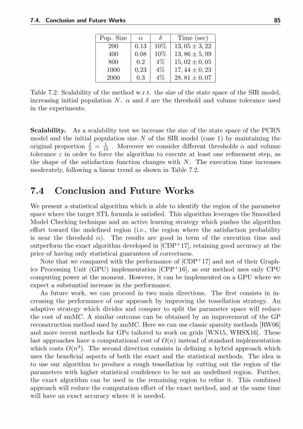
7.4. Conclusion and Future Works 85
Pop. Size α δ Time (sec)200 0.13 10% 13, 05± 3, 22400 0.08 10% 13, 86± 5, 99800 0.2 4% 15, 02± 0, 051000 0.23 4% 17, 44± 0, 232000 0.3 4% 28, 81± 0, 07
Table 7.2: Scalability of the method w.r.t. the size of the state space of the SIR model,increasing initial population N . α and δ are the threshold and volume tolerance usedin the experiments.
Scalability. As a scalability test we increase the size of the state space of the PCRNmodel and the initial population size N of the SIR model (case 1) by maintaining theoriginal proportion I
S = 119 . Moreover we consider different thresholds α and volume
tolerance ε in order to force the algorithm to execute at least one refinement step, asthe shape of the satisfaction function changes with N . The execution time increasesmoderately, following a linear trend as shown in Table 7.2.
7.4 Conclusion and Future Works
We present a statistical algorithm which is able to identify the region of the parameterspace where the target STL formula is satisfied. This algorithm leverages the SmoothedModel Checking technique and an active learning strategy which pushes the algorithmeffort toward the undefined region (i.e., the region where the satisfaction probabilityis near the threshold α). The results are good in term of the execution time andoutperform the exact algorithm developed in [CDP+17], retaining good accuracy at theprice of having only statistical guarantees of correctness.
Note that we compared with the performance of [CDP+17] and not of their Graph-ics Processing Unit (GPU) implementation [CPP+16], as our method uses only CPUcomputing power at the moment. However, it can be implemented on a GPU where weexpect a substantial increase in the performance.
As future work, we can proceed in two main directions. The first consists in in-creasing the performance of our approach by improving the tessellation strategy. Anadaptive strategy which divides and conquer to split the parameter space will reducethe cost of smMC. A similar outcome can be obtained by an improvement of the GPreconstruction method used by smMC. Here we can use classic sparsity methods [RW06]and more recent methods for GPs tailored to work on grids [WN15, WHSX16]. Theselast approaches have a computational cost of O(n) instead of standard implementationwhich costs O(n3). The second direction consists in defining a hybrid approach whichuses the beneficial aspects of both the exact and the statistical methods. The idea isto use our algorithm to produce a rough tessellation by cutting out the region of theparameters with higher statistical confidence to be not an undefined region. Further,the exact algorithm can be used in the remaining region to refine it. This combinedapproach will reduce the computation effort of the exact method, and at the same timewill have an exact accuracy where it is needed.

86 7. Parameter Synthesis
(a) Case 1(b) Zoom on Case 1
(c) Case 2 (d) Case 3
Figure 7.1: (a),(c) and (d) show the partition of the parameter space for Cases 1, 2,and 3 respectively. The positive area Pα is depicted in red, the negative area Nα is inblue and the undefined region Uα is in yellow. (a) and (c) are one dimensional case: inthe x-axis we report the parameter explored (respectively ki and kr), on the y-axis weshow the value of the satisfaction function and the confidence bounds (for βδ = 3). Thegreen horizontal line is the threshold α = 0.1 (d) shows a two dimensional parameterspace, hence no confidence bound has been represented. The circle dot represent thetraining set. In (b) we have zoomed a portion of the parameter space of (a) to visualizethe cells with base length equals to h and height equal to the span of the confidencebounds.


88 7. Parameter Synthesis

8System Design with logical
objectives
In the Introduction, we have already discussed the importance of system design. Insynthetic biology, where the experiments are costly and the analyzed processes areusually complex, a system design approach is widely applied. As typical in computer-aided engineering, this approach consists in building a model of the system of interest,in formalizing objectives to be achieved, in tuning controllable parameters to satisfythe desired goals as robustly as possible. In this chapter1 we use the logical methodsin a multi-objective fashion to perform system design of Chemical Reaction Networks(CRN) (Definition 4). The idea is to explore and discover parameters of the CRNwhich corresponds to the best trade-off between multiple requirements. We will analyzea specific case where the maximization of the satisfaction probability of two differentformulae can be effectively solved in a multi-objective paradigm (Section 4.2). Moreover,we discuss how the average robustness of this formula can be effectively used to reachthat goal but we also discuss a possible pitfall in the use of that robustness score, relatedto a difference in the scale of atomic propositions.
Related work. Multi-objective optimization techniques have been widely studied overthe last fifteen years due to their increasing importance in many academic research fields(economics, operational research, stochastic control theory, etc.) as well in industrialresearch (see [CL04]). Several solution methods exist (e.g., evolutionary algorithms[Deb01, ZQL+11], gradient optimizer with restart, single weighted sum), mostly basedon heuristic search. The multi-objective approaches to model checking verification havebeen described in [EKVY07, CMH06, FKP12]. The most common technique consistsin transforming the original problem in a linear programming problem. The systemdesign of stochastic models through the maximization of the robustness of temporalproperties is a rather new field of research [BBNS15] and in particular the multi-objectiveapproaches in this case have not been yet deeply explored.
1This contribution has been published in [BPS16].

90 8. System Design with logical objectives
8.1 Problem Formulation and Methodology
We consider the following system design problem:
given a Parametric Reaction Network (PRN) Mϑ (Definition 4), with htunable parameters ϑ = (ϑ1, . . . , ϑh) ∈ Θ ⊂ Rh and k STL formulae Φ =ϕ1, . . . , ϕk, find a value ϑ∗ ∈ Θ of the parameters such that all formu-lae are satisfied “as much as possible” (i.e., their satisfaction probability ismaximised).
There is obviously a problem here, as we have k formulae that can represent con-flicting objectives. Hence it may be impossible to maximise the satisfaction probabilityof all formulae at the same time. Moreover, different formulae can play a different role:we need to solve a multi-objective optimization problem, that is we need to estimatethe Pareto front (Section 4.2). Additionally, we have two semantics for our logic, sowe can decide to optimize either the satisfaction probability Pϕj (ϑ) or the expectationvalue of the robustness stochastic variable Rϕj (ϑ), i.e., %ϕj (ϑ) = E(Rϕj (ϑ)). Note thatboth these quantities are functions of the model parameters ϑ ∈ Θ. We consider andcompare three different approaches:
Direct probability Approach (DpA): solve directly the multi-objective problem as-sociated to the maximization of the probability
PΦ(ϑ) = (Pϕ1(ϑ), Pϕ2(ϑ), . . . , Pϕk(ϑ))
Direct robustness Approach (DrA): solve the multi-objective problem associatedto the maximization of the average robustness
%Φ(ϑ) = (%ϕ1(ϑ), %ϕ2
(ϑ), . . . , %ϕk(ϑ))
Mixed Approach(MA): combine the two approaches automatically switching amongthem
Considering our goal, the DpA seems the natural choice. However, the quantita-tive semantics carries information about the satisfiability of a formula for each trace,plus additional information about robustness of satisfaction. As discussed in [BBNS15],when we average the robustness score over all trajectories, according to the distribu-tion Pϑ on trajectories, induced by a PRN Mϑ, we typically obtain a score which ispositively correlated with the satisfaction probability. This means that, as a functionof ϑ, typically satisfaction probability increases when average robustness does (see forinstance Figure 8.1).
Furthermore, the robustness score typically carries more information in regions ofthe parameter spaces in which the satisfaction probability is flat, e.g., equal to zero orto one. In some cases, in fact, it happens that the probability vector is higher than zeroonly in a very tiny zone of the parameters space (this will be the case, for instance, inthe genetic toggle switch). The flatness of the objective vector function in a large areaof the search space is a serious challenge for the optimization process, which will beforced to explore the objective space randomly and it is likely to remain stuck in such

8.1. Problem Formulation and Methodology 91
region. In these regions, however, the robustness score is typically non-constant, hencerobustness is used to guide the optimization in these cases.
However, one can easily check that %ϕi(ϑ) > %ϕi(ϑ′) 6⇒ Pϕi(ϑ) > Pϕi(ϑ
′). Thisimplies that maximizing directly the average robustness (DrA) could produce underoptimal results. In fact, even if typically an increase in the average robustness corre-sponds to an increase in the satisfaction probability (Figure 8.1), this may fail for someparameters ϑ and ϑ′ such that %ϕi(ϑ) > %ϕi(ϑ
′) and Pϕi(ϑ) < Pϕi(ϑ′).
This discussion leads us naturally to consider mixed strategies. In the MA approach,we have modified a genetic algorithm allowing the possibility to compare two designsbased on the probability or on the robustness degree automatically. When two designshave the same probability of the STL formulae, the algorithm will automatically switchto the robustness degree. Basically, this algorithm has the possibility to switch torobustness whenever it is stuck in a plateau of the satisfaction probability vector, whichtypically happens not only when all formulae are satisfied with probability zero, but alsowith probability one (which is part of the Pareto front). In this region, the robustnessscore leads us to pick the most robust ϑ∗ satisfying the design problem.
Computing the satisfaction probability and the robustness scores. The exactcomputation of the satisfaction probability or of the expected robustness, up to a fixednumerical precision ε is unfeasible, hence we will exploit statistical methods. Morespecifically, for each fixed ϑ, we sample N trajectories Traj = x1,x2, . . . ,xN of thePRN using Gillespie’s algorithm [Gil77]. Then, for each STL formula ϕi of interest, weestimate Pϕi(ϑ) and %ϕi(ϑ) as
Pϕi(ϑ) =|x ∈ Traj | (x, 0) |= ϕi|
N; %ϕi(ϑ) =
∑kj=1 %(ϕi,xj , 0)
N
Estimating statistically the functions to optimize is computationally feasible, buthas the side effect of making their evaluation noisy, which must be taken into accountin the optimization phase. Here we try to reduce this effect by using a large number ofsimulations per point of the parameter space explored (here we used 500 runs per point,as a good trade-off between noise and computational cost). An appealing alternativewould be to rely on statistical regularization methods like Gaussian processes-basedemulation (Section 3.1), which are typically an ingredient of active learning algorithms,like Pareto Active Learning (PAL, [ZSKP13]).
The multi-objective optimization algorithm. The optimizer we have used isthe NSGA-II [DAPM02], a well known genetic algorithm largely used to solve multi-objective optimization problems, which we also introduce in Subsection 4.2.1. It com-bines mutation and crossover operators to allow the creation of new points. A com-parison procedure based on the Pareto dominance will give preference to points whichdominate the largest number of other points, pushing effectively the optimization al-gorithm towards the Pareto front. We have slightly modified the comparison process:if two points have the same probability with respect to an STL formula, the compari-son between them will be based on the robustness degree. Otherwise, the comparisonis based on the probability. This strategy permits the optimization process to easily
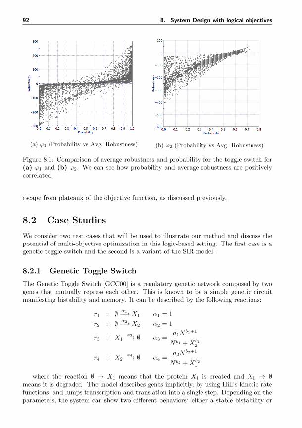
92 8. System Design with logical objectives
(a) ϕ1 (Probability vs Avg. Robustness) (b) ϕ2 (Probability vs Avg. Robustness)
Figure 8.1: Comparison of average robustness and probability for the toggle switch for(a) ϕ1 and (b) ϕ2. We can see how probability and average robustness are positivelycorrelated.
escape from plateaux of the objective function, as discussed previously.
8.2 Case Studies
We consider two test cases that will be used to illustrate our method and discuss thepotential of multi-objective optimization in this logic-based setting. The first case is agenetic toggle switch and the second is a variant of the SIR model.
8.2.1 Genetic Toggle Switch
The Genetic Toggle Switch [GCC00] is a regulatory genetic network composed by twogenes that mutually repress each other. This is known to be a simple genetic circuitmanifesting bistability and memory. It can be described by the following reactions:
r1 : ∅ α1−→ X1 α1 = 1
r2 : ∅ α2−→ X2 α2 = 1
r3 : X1α3−→ ∅ α3 =
a1Nb1+1
N b1 +Xb12
r4 : X2α4−→ ∅ α4 =
a2Nb2+1
N b2 +Xb21
where the reaction ∅ → X1 means that the protein X1 is created and X1 → ∅means it is degraded. The model describes genes implicitly, by using Hill’s kinetic ratefunctions, and lumps transcription and translation into a single step. Depending on theparameters, the system can show two different behaviors: either a stable bistability or

8.3. Results 93
rapid switching between equilibria. In the first case the system will tend to stabilize fora long time in one of the two stable equilibria, (either X1 ≥ X2 or X2 ≥ X1). In thesecond case, the system frequently switches from the state X1 ≥ X2 to X2 ≥ X1, andviceversa.
8.2.2 Epidemic model: SIRS
The SIR model [GCC00] is still widely used to simulate the spreading of a disease amonga population. The basic SIR model already introduced in Example 1 can be modifiedin many ways: considering vaccinations, introducing natural birth and death process,describing a latent phase of the disease, see [Bra08] for an overview. We consider aversion of the model described by the following set of reactions:
r1 : S + Iα1−→ 2I α1 = ksi ·
Xs ·Xi
N
r2 : Iα2−→ R α2 = kir ·Xi
r3 : Sα3−→ R+ V α3 = kv ·Xs
r4 : Iα4−→ S α4 = kis ·Xi
r5 : Rα5−→ S α5 = krs ·Xr
The population of N individuals is typically divided in three classes (though we willconsider an extra one for vaccination):
• susceptible S, representing healthy individuals that are vulnerable to the infection.
• infected I, describing individuals that have been infected by the disease and areactively spreading it.
• recovered R and vaccinated V , modelling individuals that are immune to the dis-ease, by having recovered from the disease (R), or by vaccination (V ).
Here, r1 describes the possibility that a susceptible gets the disease and becomesinfected. The reaction r2 models the recovery of an infected agent. The reaction r3
describes the possibility that susceptible becomes directly a recovered by vaccination(kv is the vaccination rate). Note that here the population V counts the total numberof vaccinated people. Finally, r4 describes the possibility that an infected individualrecovers without gaining immunity, while r5 models the loss of immunity of a recoveredindividual. Depending on the parameters ϑ = (ksi, kir, kv, kis, krs), different behaviorsof the disease could occur, such as the disease rapidly stops, or it becomes endemic, orthere are periodic cycles of infections, and so on.
8.3 Results
We discuss now two bi-objective optimization problems, one for each case study. Thestochastic systems were simulated and the STL formulae verified with the U-check tool(see. [BMS15]).
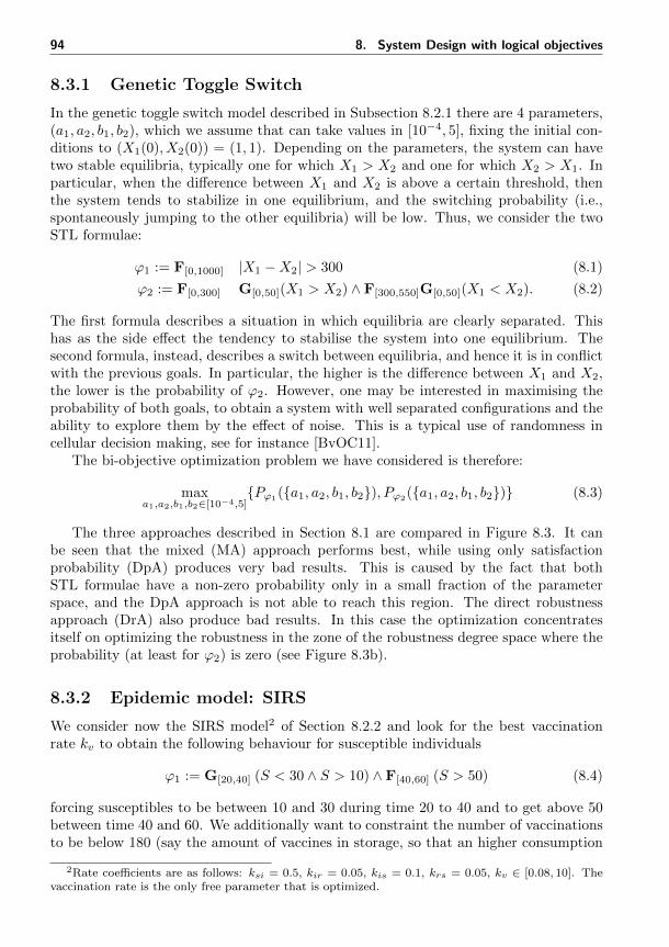
94 8. System Design with logical objectives
8.3.1 Genetic Toggle Switch
In the genetic toggle switch model described in Subsection 8.2.1 there are 4 parameters,(a1, a2, b1, b2), which we assume that can take values in [10−4, 5], fixing the initial con-ditions to (X1(0), X2(0)) = (1, 1). Depending on the parameters, the system can havetwo stable equilibria, typically one for which X1 > X2 and one for which X2 > X1. Inparticular, when the difference between X1 and X2 is above a certain threshold, thenthe system tends to stabilize in one equilibrium, and the switching probability (i.e.,spontaneously jumping to the other equilibria) will be low. Thus, we consider the twoSTL formulae:
ϕ1 := F[0,1000] |X1 −X2| > 300 (8.1)
ϕ2 := F[0,300] G[0,50](X1 > X2) ∧ F[300,550]G[0,50](X1 < X2). (8.2)
The first formula describes a situation in which equilibria are clearly separated. Thishas as the side effect the tendency to stabilise the system into one equilibrium. Thesecond formula, instead, describes a switch between equilibria, and hence it is in conflictwith the previous goals. In particular, the higher is the difference between X1 and X2,the lower is the probability of ϕ2. However, one may be interested in maximising theprobability of both goals, to obtain a system with well separated configurations and theability to explore them by the effect of noise. This is a typical use of randomness incellular decision making, see for instance [BvOC11].
The bi-objective optimization problem we have considered is therefore:
maxa1,a2,b1,b2∈[10−4,5]
Pϕ1(a1, a2, b1, b2), Pϕ2(a1, a2, b1, b2) (8.3)
The three approaches described in Section 8.1 are compared in Figure 8.3. It canbe seen that the mixed (MA) approach performs best, while using only satisfactionprobability (DpA) produces very bad results. This is caused by the fact that bothSTL formulae have a non-zero probability only in a small fraction of the parameterspace, and the DpA approach is not able to reach this region. The direct robustnessapproach (DrA) also produce bad results. In this case the optimization concentratesitself on optimizing the robustness in the zone of the robustness degree space where theprobability (at least for ϕ2) is zero (see Figure 8.3b).
8.3.2 Epidemic model: SIRS
We consider now the SIRS model2 of Section 8.2.2 and look for the best vaccinationrate kv to obtain the following behaviour for susceptible individuals
ϕ1 := G[20,40] (S < 30 ∧ S > 10) ∧ F[40,60] (S > 50) (8.4)
forcing susceptibles to be between 10 and 30 during time 20 to 40 and to get above 50between time 40 and 60. We additionally want to constraint the number of vaccinationsto be below 180 (say the amount of vaccines in storage, so that an higher consumption
2Rate coefficients are as follows: ksi = 0.5, kir = 0.05, kis = 0.1, krs = 0.05, kv ∈ [0.08, 10]. Thevaccination rate is the only free parameter that is optimized.

8.3. Results 95
(a) Probability Space (b) Robustness Space
Figure 8.2: Comparison of the three optimization approaches for the SIRS model. Thered squared dots represent the MA approach, the blue triangular dots represent theDrA approach and the green circular dots are referred to the DpA. Chart (a) shows alldesigns, with larger dots representing the Pareto fronts of the referred approaches. In(b) we have represented the same dots respect to the robustness degree space. Unlikethe Toggle Switch example, the three approaches produce comparable results.
(a) Satisfaction Probability (b) Robustness Degree
Figure 8.3: Comparison of the three optimization approaches for the toggle switch. Thered squared dots represent the MA approach, the blue triangular dots represent theDrA approach and the green circular dots are referred to the DpA. Chart (a) shows alldesigns, with larger dots representing the Pareto fronts of the referred approaches. In(b) we have represented the same dots respect to the robustness degree space.

96 8. System Design with logical objectives
(a) Probability Space (b) Robustness Space
Figure 8.4: Comparison of the Pareto front of the SIRS model, obtained by maximizingthe robustness and the probability. The Pareto front obtained by maximizing the prob-ability (green circular designs) dominates the Pareto front obtained by maximizing therobustness (blue triangular designs).
forces to buy new vaccines), which we enforce with the following goal
ϕ2 := G[0,250] (V < 180) (8.5)
Differently from the Toggle Switch scenario, the three optimization approaches havesimilar performances, as shown in Figure 8.2. The reason is that the satisfaction prob-ability of both ϕ1 and ϕ2 is non-zero in a large portion of the state space, and thecorrelation between probability and robustness is larger than for the toggle switch.
8.4 A deeper look at robustness
In this section we focus our attention on the robustness score associated with a formula,starting from a potential criticism to multi-objective optimization. Logic formulae canbe combined, for instance by Boolean connectives. Hence, if we have two formulae, ϕ1
and ϕ2, representing two potentially conflicting objectives, we can take their conjunctionand solve the single objective optimization for ϕ1∧ϕ2, e.g., with the method of [BBNS15]which uses the robustness score. Even if the two approaches are not directly comparableconsidering that they solve different tasks (see. [Deb14]), the second approach could beappealing for computational reasons.
However, consider the following scenario: let ϕ1, ϕ2 and ψ := ϕ1 ∧ ϕ2 such that∀ϑ ∈ Θ, %ϕ1
(ϑ) ∈ [a, b] and %ϕ2(ϑ) ∈ [c, d] where a, b, c, d ∈ R and b c. Clearly ∀ϑ ∈
Θ, %ψ(ϑ) = min(%ϕ1(ϑ), %ϕ2
(ϑ)) = %ϕ1(ϑ), hence optimizing the robustness, we would
completely ignore %ϕ2(ϑ). As a less artificial example, we have compared these multi-
objective and single-objective approaches applied to the maximization of the averagerobustness of the SIRS model (see Subsection 8.3.2 and Subsection 8.2.2) with respect
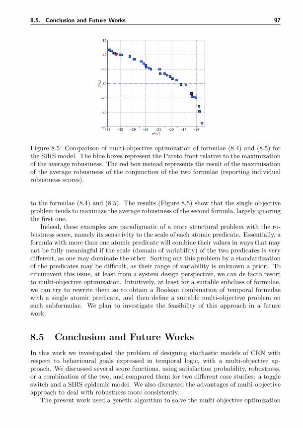
8.5. Conclusion and Future Works 97
Figure 8.5: Comparison of multi-objective optimization of formulae (8.4) and (8.5) forthe SIRS model. The blue boxes represent the Pareto front relative to the maximizationof the average robustness. The red box instead represents the result of the maximisationof the average robustness of the conjunction of the two formulae (reporting individualrobustness scores).
to the formulae (8.4) and (8.5). The results (Figure 8.5) show that the single objectiveproblem tends to maximize the average robustness of the second formula, largely ignoringthe first one.
Indeed, these examples are paradigmatic of a more structural problem with the ro-bustness score, namely its sensitivity to the scale of each atomic predicate. Essentially, aformula with more than one atomic predicate will combine their values in ways that maynot be fully meaningful if the scale (domain of variability) of the two predicates is verydifferent, as one may dominate the other. Sorting out this problem by a standardizationof the predicates may be difficult, as their range of variability is unknown a priori. Tocircumvent this issue, at least from a system design perspective, we can de facto resortto multi-objective optimization. Intuitively, at least for a suitable subclass of formulae,we can try to rewrite them so to obtain a Boolean combination of temporal formulaewith a single atomic predicate, and then define a suitable multi-objective problem onsuch subformulae. We plan to investigate the feasibility of this approach in a futurework.
8.5 Conclusion and Future Works
In this work we investigated the problem of designing stochastic models of CRN withrespect to behavioural goals expressed in temporal logic, with a multi-objective ap-proach. We discussed several score functions, using satisfaction probability, robustness,or a combination of the two, and compared them for two different case studies: a toggleswitch and a SIRS epidemic model. We also discussed the advantages of multi-objectiveapproach to deal with robustness more consistently.
The present work used a genetic algorithm to solve the multi-objective optimization

98 8. System Design with logical objectives
problem. We have modified its comparison criterion in order to use a combinationof satisfaction probability and robustness degree. We plan to investigate the use ofstatistically more refined optimization methods to deal with noise in the estimationof the objective function due to the use of simulation, like Pareto Active Learning[ZSKP13]. This will allow us to reduce the number of simulation runs per point of theparameter space, thus improving complexity.

9Falsification of Cyber-Physical
Systems
Model-based Development (MBD) is a well known design framework of complex engi-neered systems, concerned with reducing cost and time of the prototyping process. Mostprominently, this framework has been adopted in the industrial fields such as automotiveand aerospace where the conformity of the end product is extremely important. The ma-jority of systems in these areas are Cyber-Physical Systems (CPS) [LS16] (Section 1.1),where physical and software components interact producing complex behaviors. Thesesystems can be described by appropriate mathematical models which are able to cap-ture all the system behaviors. Moreover, it is necessary to have a suitable specificationframework capable of analyzing the output of such models.
Hybrid systems [MMP91] are the mathematical framework usually adopted, whiletemporal logic (Chapter 2), due to its ability to describe temporal events, is generallyused as specification framework. The high level of expressivity of hybrid systems, whichis the main reason for their success, is also the cause of their undecidability, even forsimple logic formulae. Subclasses of hybrid systems which are decidable for specifictemporal logic formulae exist and have been widely studied during the last 15 years, aswell as model checking techniques capable of verifying them [ACH+95]. Unfortunately,the majority of CPS used nowadays in the industrial field are much more complex thandecidable hybrid systems. They are mainly described by using block diagram tools (i.e.,Simulink/Stateflow, Scade, LabVIEW, and so on) where several switch blocks, 2/3-Dlook-up tables and state transitions coexist. These CPS are generally not decidable andstandard model checking techniques are not feasible, leading to the proposal of differenttechniques [ALFS11b].
Testing procedures with the purpose of verifying the model on specific behaviors havebeen adopted for several years. These are feasible approaches whenever it is possible towrite in advance collections of test cases which extensively cover all the possible eventsleading to system failure [Vin98]. With the increase of complexity, such an a prioriassumption is not viable in most of the real cases and for this reason different techniques,such as random testing and search-based testing, have been introduced [ZKH03]. The

100 9. Falsification of Cyber-Physical Systems
general idea consists in expressing the falsification procedure as an optimization processaiming at minimizing a target quantity which describes “how much a” given property isverified. For example, achieving a negative value of the robustness semantics of a givenSignal Temporal Logic (STL) [DM10] formula means falsifying the system with respectto that formula.
Related Work. Different approaches have been proposed to achieve the falsificationof black box models, starting from test based approaches until recently, when search-based test approaches have become more popular. Stochastic local search [DJKM15],probabilistic Monte Carlo [AFS+13] and mixed coverage/guided strategy [DDD+15] ap-proaches have been proposed and benchmark problems created [JDK+14, HAF14]. Twosoftware packages [Don10, ALFS11b] implement the aforementioned techniques. Boththese software tools assume a fix parameterization of the input function, differently fromus. Similarly to our approach, in [DDD+15] and [DJKM15] the fixed parameterizationis avoided. More specifically in [DDD+15] no parameterization has been used at all andthe input signals are modified on the fly based on the robustness of the partial systemtrajectories. In [DJKM15] a uniform discretization of the input domains (both timeand values) is dynamically applied to discretize the search space. The use of Gaussianprocesses for falsification has been adopted in [Aka16] but it is restricted to conditionalsafety properties.
Contribution. In this chapter1 we study the falsification problem of black box sys-tems (i.e., block diagram models such as Simulink/Stateflow model or sets of ordinarydifferential equations generally used in automotive or aerospace industrial fields) whichtakes as input and produce as output continuous or piecewise continuous (PWC) sig-nals. The requirements are expressed by using STL. Solving such falsification problemsin a search-based framework poses two main challenges. Generally, the simulation ofblock diagram models is time consuming, hence it is necessary to falsify the model withas few simulations as possible. Moreover, the models accept continuous and/or PWCsignals as inputs and an efficient finite dimensional parametrization is necessary to per-form an optimization procedure. The contribution we propose in this work is to tacklethese challenges by a novel strategy leveraging machine learning techniques (Gaussianprocesses and active learning) and by using a new adaptive version of the control pointsparameterization approach.
9.1 Domain Estimation with Gaussian Processes
We now define the domain estimation problem and solve it by using Gaussian processes.In this section we describe how to cast the falsification problem into a domain estimationproblem.
Definition 23. Consider a function f : D → R, where D ⊆ Rk is a general domainspace, and an interval I = [a, b] ⊆ R. We define the domain estimation problem as the
1This contribution has been published in [SPB17b].

9.2. The Falsification Process 101
task of identifying the set B of points x ∈ D such that f(x) ∈ I:
B = x ∈ D | f(x) ∈ I ⊆ D, (9.1)
In practice, if B 6= ∅, we will limit us to identify a subset B ⊆ B of size n.
Gaussian Processes (GP) can be efficiently used to solve this task. Similarly to thecross-entropy methods for optimization [RK13], the idea is to implement an iterativesample strategy in order to increase the probability to sample a point in B, as thenumber of iterations increases. Consider the set K(f) = (xi, f(xi) )i≤n representingthe partial knowledge we have collected after n iterations and the Gaussian processfK(x) ∼ GP (mK(x), σK(x)) trained on K(f). We can easily estimate P (x ∈ B) =P (fK(x) ∈ I), where I = [a, b], by computing the probability of a Gaussian distributionwith mean mK(x) and variance σ2
K(x) as follows
P (x ∈ B) = Φ
(b−mK(x)
σK(x)
)− Φ
(a−mK(x)
σK(x)
)(9.2)
This2 corresponds to our uncertainty on the value of f(x) belonging to I, as capturedby the GP reconstruction of f . The previous probability can be effectively used to solvethe domain estimation problem described in Definition 23. Our approach is describedin Algorithm 7. The idea is to use P (fK(x) ∈ I) to guide the sampling.
• During initialization (line 1), we set the iteration counter (i) and the minimumdistance (d) from the interval I. The set (B) containing the elements of (B) isset to empty ensuring that the algorithm is run at least once. The knowledge setK(f) is initialized with some randomized points sampled from D (line 2).
• In the iterative loop (line 3), the algorithm first checks if the number of coun-terexamples (ce) or maximum number of iterations (maxIter) has been reached.In this case, the method stops returning the estimated set (B) and the minimumdistance from I that has been registered until that point. Otherwise new GPsare trained by using K(f) (line 4) and a set composed by m points (Dgrid) isgenerated by a Latin Hypercube sampling [MBC79], so to have a homogeneousdistribution of points in space (line 5). For each of these points x, the probabilityP (x ∈ B) = P (fK(x) ∈ I) is evaluated and the set (x, P (x ∈ B)), x ∈ Dgrid isthen created. Afterwards, a candidate point xnew is sampled from Dgrid propor-tionally to its associated probability (line 6) so to increase the sampling of pointswith higher estimated probability of belonging to B. Consequently, K(f) is up-graded and if x ∈ B then x is added to B (line 11). The procedure outputs alsod, the minimum distance of the evaluated points from the interval I calculatedduring the procedure.
9.2 The Falsification Process
We adopt a black box optimization approach, meaning that we consider the targetblock diagram model as a black box dynamical systemM = U×X, sim (see Subsec-
2Φ is the CDF of the standard normal distribution.

102 9. Falsification of Cyber-Physical Systems
Algorithm 7 domainEstimation algorithm
Require: maxIter, ce,m, f, I1: i← 0, B ← ∅, d← +∞2: initialize(K(f))3: while ( |B| ≤ ce and i ≤ maxIter) do4: fK(f) ∼ trainGaussianProcess(K(f))5: Dgrid ← lhs(m)6: xnew ← sample(x, P (x ∈ B)), x ∈ Dgrid7: fnew ← f(xnew)8: d← min(d,distance(fnew, I))9: K(f)← K(f) ∪ (xnew, fnew)
10: if fnew ∈ I then11: B = B ∪ xnew12: end if13: i← i+ 114: end while
tion 1.3.3).A big effort during the prototyping process consists in verifying the requirements
usually expressed as safety property, such as:
∀(u, x0) ∈ UT ×X0 , %(ϕ, (u,x), 0) > 0 (9.3)
meaning that for each input function and initial state x0 ∈ X0 ⊆ X, the dynamics ofthe systems represented by the couple (u,x), where u ∈ UT is the input function andx ∈ XT is the state function, satisfies the STL formula ϕ. It is possible to interpret thesafety condition (9.3) as a domain estimation problem associated with
B = (u, x0) ∈ UT ×X0 , %(ϕ, (u,x), 0) < 0 (9.4)
with the purpose of verifying its emptiness, which entails that (9.3) is satisfied. We callB the counterexample set and its elements counterexamples.
Solving the previous domain estimation problem could be extremely difficult becauseof the infinite dimensionality of the input space, which is a space of functions. For thisreason, it is mandatory to parameterize the input function by means of an appropriatefinite dimensional representation.
Let us consider for simplicity that U = U1 × · · · × Um, where m < +∞. One ofthe most used parameterization—mainly for its simplicity—is the fixed control pointparameterization (fixCP): after having fixed the times (tk1 , . . . , t
knk
), the control points
(tk1 , uk1), . . . , (tknk , uknk
) are chosen as parameter of the k-th input signals. We also needto choose an interpolation set of function with nk degrees of freedom for each k-th inputsignals (Fknk ⊂ T → Uk, e.g., piecewise linear, polynomials of degree nk, and so on(see [SF12])), the fixCP parameterization will associate with each control point ck =(tk1 , uk1), . . . , (tknk , u
knk
) the unique function Fck ∈ Fknk satisfying ∀i ≤ n , Fck(tki ) = uki .Let us denote by Fn = (F1
n1, . . . ,Fmnm) the set of interpolating functions.
It is clear that by increasing the number of control points, we will enlarge the set

9.2. The Falsification Process 103
of approximant functions Fn: n ≤ m implies Fn ⊂ Fm, where n ≤ m is intendedpointwise. As piecewise linear or polynomial functions are known to be dense in thespace of continuous functions, by choosing an appropriately large n, we can approximateany input function with arbitrary precision.
Considering an n-fixCP, which is a fixCP where n = (n1, . . . , nm) represents thenumber of control points used for each input variables, it is possible to introduce thedomain estimation problem (9.4) associated with the following set:
B = (c, x0) ∈ Un11 × · · · × Unmm × X0, %(ϕ, (Fn(c), x), 0) < 0 (9.5)
which , differently from (9.4), is a finite dimensional set described by using∑mj=1 nj +
dim(X0) variables.By the density argument it is clear that
(9.4) has at least one element ⇐⇒ ∃n ∈ ωm, (9.5) has at least one element
A possible strategy is to solve the domain estimation problem associated with (9.5)by choosing the minimum n such that Fn × X0 contains a counterexample. Applyingthat strategy, even in simple cases, could be cumbersome as shown in the followingexample.
Toy example. Consider a simple black box model which accepts a single piecewiseconstant function u : [0, 1] → [0, 1] as input function and returns the same functionx = u as output. Considering the following requirement ϕ := ¬(G[0,0.51] 0 < x <0.2∧G[0.55,1] 0.8 < x < 1), it is evident that it could be falsified only in a control pointparameterization having at least the point (ti, ui) such that ti ∈ [0.51, 0.55]. Otherwiseif this points does not exists it means the output signals will assume a constant valuein [0.51, 0.55] which implies that or G[0.55,1] (0.8 < x < 1) or G[0,0.51] (0 < x < 0.2) isfalse, meaning that ϕ is not falsified. The minimum number of uniformed fixed controlpoints necessary to achieve it is 9, which entails a considerable computational effort.
A natural way to overcome the limitation of the fixCP consists in considering thetimes of the control points as variables. An n-adaptive Control Points parameterization(n-adaCPP) consists in a function F knk : Tnk × Unkk → Fknk , which has twice as muchparameters than the fixed version: values at control points and times (which are con-strained by ∀i < n ti ≤ ti+1). The adaptive parameterization is preferable with respectto the fixed one because of its ability to describe functions with local high variabilityeven with a low number of control points. In fact it is possible to concentrate any frac-tion of the available control points in a small time region, inducing a large variation inthis region, while letting the parameterized function vary much less outside it.
9.2.1 Adaptive Optimization
The idea of the adaptive optimization approach consists in falsifying (9.3) starting froma simple input function and increasing its expressiveness by increasing the number ofcontrol points. After having defined a parameterization for each of the m input signals(which compose the input function u), Algorithm 8 works as following:

104 9. Falsification of Cyber-Physical Systems
• At the first iteration a parameterization Fn0 = F 01 , . . . , F
0n with zero control
points for each signals (n0 = (0, . . . , 0)) is considered (line 1). Zero control pointsmeans defining input signals which are constant functions. The final counterex-ample set (B) is set to empty, which ensures the optimization is run at least once(line 2).
• In the iterative loop, the algorithm first checks if the number of counterexamples(ce) or if the maximum global number of iterations (mgi) has been reached. In thiscase, the method stops returning the counter example set (B). Otherwise, the fal-sification problem is solved by using the domain estimation procedure domainEs-timation (Algorithm 7) which returns the counterexample set and the minimumvalue of the robustness found by using that parameterization (see Section 9.1 fordetails). The parameterization is then expanded by picking a coordinate of theinput signal (line 5 - 9) and adding a new control point (line 10), obtaining a newparameterization Fni+1
.
Algorithm 8 adaptiveGPFalsification algorithm
Require: mgi,mii, ce,m, ϕ1: Input: mgi,mii, ce,m, ϕ2: n0 ← (0, . . . , 0)3: B ← ∅, k0 ← 0, i← 0, d0 ← +∞4: while (|B| ≤ ce and i ≤ mgi) do5: [B−, di+1] = domainEstimation(mii,ni, ce− |B|,m, %(ϕ, ·, t), (−∞, 0))6: if di+1 > di then7: ki+1 ← ki8: else9: ki+1 ← (ki + 1) mod n
10: end if11: ni+1 ← ni + ek12: i← i+ 113: B ← B ∪B−14: end while
The general idea of this approach is to keep low the number of parameters by startingfrom constant signal and gradually increasing the number of control points of the inputfunctions. In the adaptive control points parameterization, adding a control point meansadding two new degrees of freedom (one for the time and one for the value of the controlpoint). This means, on the one hand, having more expressiveness and so more chancesto falsify the system, but on the other hand this complicates the optimization processand increases the dimension of the search space as well, hence, the minimum number ofsimulations required to solve it. For this reason it is convenient to add control pointsonly where it is truly necessary.
9.3. Probabilistic Approximation Semantics 105
9.3 Probabilistic Approximation Semantics
Gaussian processes can be used to estimate the probability that a given input falsifiesa system as described in Section 9.1 and Section 9.2. This fact offers the possibility todefine an approximate semantics which generalizes the concept of probability of falsifi-cation that we can infer considering the knowledge of the system we have collected. Thebasic idea is to decompose an STL formula as a Boolean combination of temporal modal-ities, propagating the probability of the temporal operators, estimated by GPs, throughthe Boolean structure. Formally, let L0 be the subset of STL containing only atomicpropositions and temporal formulae of the form ϕ1U[T1,T2]ϕ2, F[T1,T2]ϕ and G[T1,T2]ϕ,that cannot be equivalently written as Boolean combinations of simpler formulae. Forexample FT (ϕ1∨ϕ2) is not in L0 because FT (ϕ1∨ϕ2) ≡ FTϕ1∨FTϕ2. Furthermore, letL be the logic formed by the Boolean connective closure of L0. Clearly L is isomorphicto STL. 3
For simplicity, let us denote by ϑ a parameter and describe the input function byuϑ and the initial state by x0ϑ. We write xϑ to indicate the path generated by thesimulator, given as input uϑ and x0ϑ, according to Section 1.3.3. We want to define an(approximate) semantics giving the probability that a path xϑ satisfies a given formulaψ ∈ L (without simulating it). The idea is to evaluate the quantitative semantics ofthe atomic formulae ϕj ∈ L0 of ψ on a finite collection of parameters (ϑii≤n), thenbuilding GPs in order to estimate the probability that the quantitative semantics of eachformula ϕj is higher than zero on a target parameter. This is again a Domain EstimationProblem (Section 9.1), where the function is the robustness associated with the STLformula ϕj and the interval I is (0,+∞). We propagate this probability through theBoolean structure of ψ according to the following:
Definition 24 (Probabilistic Approximation Semantics of L). The probabilistic approx-imation function γ : L ×UT × [0,∞)→ [0, 1] is defined by:
• γ(ϕ, ϑ, t) = P (fK(ϕ)(ϑ) > 0)
• γ(¬ψ, ϑ, t) = 1− γ(ψ, ϑ, t)
• γ(ψ1 ∧ ψ2, ϑ, t) = γ(ψ1, ϑ, t) ∗ γ(ψ2, ϑ, t)
• γ(ψ1 ∨ ψ2, ϑ, t) = γ(ψ1, ϑ, t) + γ(ψ2, ϑ, t)− γ(ψ1 ∧ ψ2, ϑ, t)
where K(ϕ) = ϑi, %(ϕ, ϑi, t)i=1,..,n is the partial knowledge of the satisfiability of ϕ ∈L0 that we have collected performing n simulations for parameters (ϑi)i=1,..,n. fK(ϕ) isthe GP trained on K(ϕ), and P refers to its probability. For simplicity we use γ(ψ, ϑ, t)to mean γ(ψ, (uϑ, xϑ), t).
In the previous definition, the probability P (fK(ϕ)(ϑ) > 0) is easily computed, asfK(ϕ)(ϑ) is normally distributed.
Including the Probabilistic Approximation Semantics (PAS) in our falsification pro-cedure (Algorithm 8) is straightforward. Given the formula we have to falsify, first wenegate and decompose it in order to identify the L formula and ist atom in L0 associated
3ϕ ∈ L iff ψ := ϕ | ¬ψ |ψ ∨ ψ |ψ ∧ ψ, with ϕ ∈ L0.
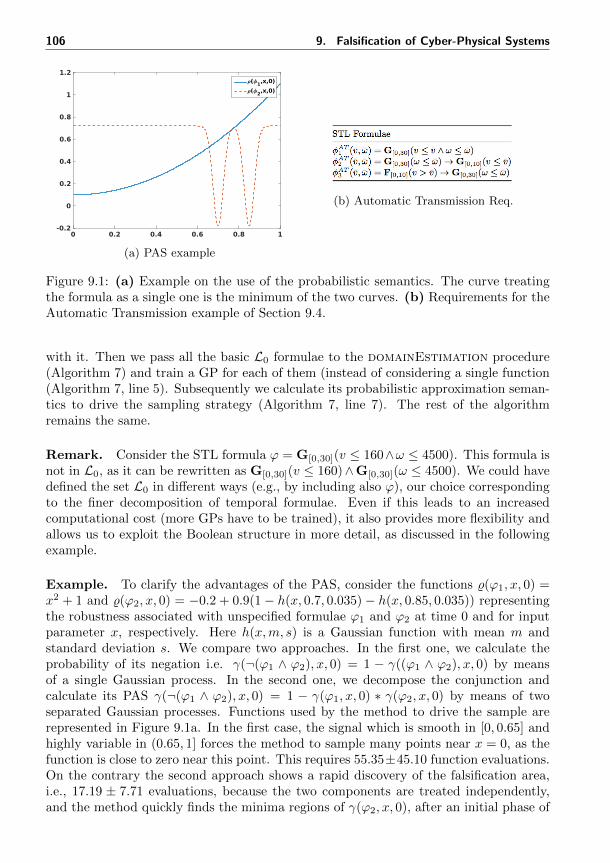
106 9. Falsification of Cyber-Physical Systems
(a) PAS example
(b) Automatic Transmission Req.
Figure 9.1: (a) Example on the use of the probabilistic semantics. The curve treatingthe formula as a single one is the minimum of the two curves. (b) Requirements for theAutomatic Transmission example of Section 9.4.
with it. Then we pass all the basic L0 formulae to the domainEstimation procedure(Algorithm 7) and train a GP for each of them (instead of considering a single function(Algorithm 7, line 5). Subsequently we calculate its probabilistic approximation seman-tics to drive the sampling strategy (Algorithm 7, line 7). The rest of the algorithmremains the same.
Remark. Consider the STL formula ϕ = G[0,30](v ≤ 160∧ω ≤ 4500). This formula isnot in L0, as it can be rewritten as G[0,30](v ≤ 160)∧G[0,30](ω ≤ 4500). We could havedefined the set L0 in different ways (e.g., by including also ϕ), our choice correspondingto the finer decomposition of temporal formulae. Even if this leads to an increasedcomputational cost (more GPs have to be trained), it also provides more flexibility andallows us to exploit the Boolean structure in more detail, as discussed in the followingexample.
Example. To clarify the advantages of the PAS, consider the functions %(ϕ1, x, 0) =x2 + 1 and %(ϕ2, x, 0) = −0.2 + 0.9(1− h(x, 0.7, 0.035)− h(x, 0.85, 0.035)) representingthe robustness associated with unspecified formulae ϕ1 and ϕ2 at time 0 and for inputparameter x, respectively. Here h(x,m, s) is a Gaussian function with mean m andstandard deviation s. We compare two approaches. In the first one, we calculate theprobability of its negation i.e. γ(¬(ϕ1 ∧ ϕ2), x, 0) = 1 − γ((ϕ1 ∧ ϕ2), x, 0) by meansof a single Gaussian process. In the second one, we decompose the conjunction andcalculate its PAS γ(¬(ϕ1 ∧ ϕ2), x, 0) = 1 − γ(ϕ1, x, 0) ∗ γ(ϕ2, x, 0) by means of twoseparated Gaussian processes. Functions used by the method to drive the sample arerepresented in Figure 9.1a. In the first case, the signal which is smooth in [0, 0.65] andhighly variable in (0.65, 1] forces the method to sample many points near x = 0, as thefunction is close to zero near this point. This requires 55.35±45.10 function evaluations.On the contrary the second approach shows a rapid discovery of the falsification area,i.e., 17.19 ± 7.71 evaluations, because the two components are treated independently,and the method quickly finds the minima regions of γ(ϕ2, x, 0), after an initial phase of

9.4. Case Studies 107
Adaptive PAS Adaptive GP-UCB S-TaLiRo
Req nval times nval times nval times Alg
ϕAT1 (160, 4500) 4.42± 0.53 2.16± 0.61 4.16± 2.40 0.55± 0.30 5.16± 4.32 0.57± 0.48 URϕAT1 (160, 4765) 6.90± 2.22 5.78± 3.88 8.7± 1.78 1.52± 0.40 39.64± 44.49 4.46± 4.99 SAϕAT2 (75, 4500) 3.24± 1.98 1.57± 1.91 7.94± 3.90 1.55± 1.23 12.78± 11.27 1.46± 1.28 CEϕAT2 (85, 4500) 10.14± 2.95 12.39± 6.96 23.9± 7.39 9.86± 4.54 59± 42 6.83± 4.93 SAϕAT2 (75, 4000) 8.52± 2.90 9.13± 5.90 13.6± 3.48 4.12± 1.67 43.1± 39.23 4.89± 4.43 SAϕAT3 (80, 4500) 5.02± 0.97 2.91± 1.20 5.44± 3.14 0.91± 0.67 10.04± 7.30 1.15± 0.84 CEϕAT3 (90, 4500) 7.70± 2.36 7.07± 3.87 10.52± 1.76 2.43± 0.92 11± 9.10 1.25± 1.03 UR
Table 9.1: Results. All the times are expressed in seconds. Legend - nval: numberof simulations, times: time needed to falsify the property, Alg: the algorithm used asdescribed in Section 9.4.
homogeneous exploration. In addition, the paraboloid γ(ϕ1, x, 0) is smooth and requiresfew evaluations for a precise reconstruction.
9.4 Case Studies
In this section we discuss a case study to illustrate our approach, taken from [SF12].We will compare and discuss the performance of a prototype implementation in Mat-lab of our approach with S-TaLiRo toolbox [FSUY12]. We use S-TaLiRo to computethe robustness, and the implementation of Gaussian Process regression provided byRasmussen and Williams [RN10].
Automatic Transmission (AT). We consider a Simulink model of a Car AutomaticGear Transmission Systems. There are two inputs: the throttle and the brake angledynamics describing the driving style. Modes have two continuous state variables, de-scribing vehicle (v) and engine (ω) speed. The Simulink model is initialized with afixed initial state (w0, v0) = (0, 0), it contains 69 blocks (2 integrators, 3 look-up tables,Stateflow Chart, . . . ). The requirements are described by means of STL formulae asreported in Figure 9.1b. The first requirement (ϕAT1 ) is a so called invariant, whichsays that in the next 30 seconds the engine and vehicle speed never reach ω rpm andv km/h, respectively. The second requirement (ϕAT2 ) says that if the engine speed isalways less than ω rpm, then the vehicle speed can not exceed v km/h in less than 10seconds. Finally, the third requirement (ϕAT3 ) basically says that if within 10 secondsthe vehicle speed is above v km/h then from that point on the engine speed is alwaysless than ω rpm.
Results. We analyze the performance of our approach in terms of the minimum num-ber of simulations and computational time needed to falsify the previous test cases.We have performed 50 optimization runs for each STL formula and compared its per-formance with the best statistics achieved among a Cross Entropy (CE), MontecarloSampling (SA) and Uniform Random Sampling (UR) approaches performed with the S-TaLiRo tool [ALFS11b] and the GP-UCB algorithm applied to falsification as describedin [Aka16]. As the table shows, our approach (Adaptive PAS) has good results in terms
108 9. Falsification of Cyber-Physical Systems
of the minimum number of evaluations needed to falsify the systems with respect tothe STL formulae, outperforming in almost all tests the methods of the S-TaLiRo suiteand the Adaptive GP-UCB approach. This is the most representative index, as in realindustrial cases the simulations can be considerably expensive (i.e., cases of real mea-surements on power bench, time and computation intensive simulations). In these casesthe total computational time is directly correlated with the number of simulations andthe time consumed by the optimizer to achieve its strategy becomes marginal. Further-more, we are testing our method with a prototype implementation which has not beenoptimized, in particular for what concerns the use of Gaussian processes. Despite this,the numerical results in terms of the minimum number of simulations are outperformingS-TaLiRo and GP-UCB approach.
Conditional Safety Properties. When we define a conditional safety property i.e.GT (ϕcond → ϕsafe) we would like to explore cases in which the formula is falsified butthe antecedent condition holds (see [Aka16]). This is particularly relevant when theformula cannot be falsified, as it reduces the search space, ignoring regions where theformula is trivially true due to a false antecedent. Focusing on the region where ϕcondholds requires a straightforward modification of the sampling routine of the DomainEstimation Algorithm (Algorithm 7, line 6-7). Instead of performing the samplingdirectly on the input provided by the Latin Hypercube Sampling Routine (Algorithm 7,line 6), we previously define a set of inputs verifying the antecedent condition (by thestandard Domain Estimation Algorithm using the Gaussian processes trained on therobustness of the antecedent condition) and then we sample from this set the candidatepoint (Algorithm 7, line 7).
To verify the effectiveness of this procedure we consider the STL formula G[0,30](ω ≤3000 → v ≤ 100) which cannot be falsified by any configuration of the AT model. Wetray to falsify it and calculate the percentage of sampled inputs satisfying its antecedentcondition (i.e., ω ≤ 3000). This percentage is 43% for the GP-UCB algorithm, butincreases to 87% for the modified domain estimation algorithm.
9.5 Conclusion and Future Works
In this chapter, we propose an adaptive strategy to find bugs in black box systems.We search in the space of possible input functions, suitably parameterized in order tomake it finite dimensional. We use a separate parameterization for each different inputsignal, and we use an adaptive approach, increasing gradually the number of controlpoints as the search algorithm progresses. This allows us to solve falsification problemsof increasing complexity, looking first for simple functions and then for more and morecomplex ones. The falsification processes are then cast into the domain estimation prob-lem framework, which uses the Gaussian Processes (GP) to constructs an approximateprobabilistic semantics of STL formulae, giving high probability to regions where theformula is falsified. The advantage of using such an approach is that it leverages theBayesian emulation providing a natural balance between exploration and exploitation,which are the key ingredients in a search-based falsification algorithm. In addition to anovel use of GP, we also rely on a new adaptive parameterization, treating the time ofeach control point as a variable, thus leading to an increase in expressiveness and flexi-

9.5. Conclusion and Future Works 109
bility, as discussed in Section 9.2. Moreover with a slight modification of our algorithmwe efficiently manage the falsification of the conditionsl safety properties, increasing theefficiency of the usual GP-UCB algorithm in focussing the search on the region of pointssatisfying the antecedent.
The experimental results are quite promising, particularly as far as the number ofsimulations required to falsify a property is concerned, which is lower than other ap-proaches. The computational time of the current implementation, however, is in somecases higher than S-TaLiRo. The main problem is in the cost of computing predictionsof the function emulated with a GP. This cost, in fact, is proportional to the numberof already evaluated inputs used to train the GP. To reduce this cost, we can leveragethe large literature about sparse representation techniques for GP [RW06]. Further-more, with the increase in the number of control points, we face a larger dimensionalsearch space, reflecting in an increased number of simulations needed to obtain an ac-curate representation of the robustness for optimization, with a consequent increase ofcomputational time. We can partially improve on this problem, typical of naive imple-mentations of the Bayesian approach, by refining the choice of the covariance functionand/or constraining some of its hyperparameters so as to increment the explorationpropensity of the search. In the future, we also plan to improve the adaptive approachwhich is in charge of increasing the control points of an input signal, with the goal ofdropping control points that are not useful. In the current work, we use the GP-basedsampling scheme to deal efficiently with falsification. However, our approach can bemodified to deal with the coverage problem [DDD+15], i.e., the identification of a givennumber of counterexamples which are homogeneously distributed in the falsification do-main. Our idea is to modify the sampling algorithm (Algorithm 7, line 7) by adding amemory of already visited areas, so to distribute samples homogeneously in space.


Concluding Remarks
This thesis combines formal methods and machine learning approaches to face the newchallenges of model-based development. Our research starts from the consideration thateven if formal methods are currently used in some specific areas, they are not used inmany others where they might be successfully applied. As already discussed in the In-troduction, the motivations are somewhat complex. First, there is a lack of knowledgein this area of computer science, for example, many engineers do not even encounterthem in their academic studies. Second, standard model checking techniques are notable to deal with real industrial cases. In this thesis, machine learning approaches havebeen used to make formal methods applicable even in complex industrial scenarios byincluding, in addition, some common requirements of this context, such as the blackbox modeling and the minimization of the computational cost derived from model sim-ulations.
Conclusions and future works have been already discussed at the end of each contri-bution. In this final chapter, we would like to focus on some section of this thesis whichwe think are more interesting, give some future directions and a critic review of somecontributions.
Signal convolution logic, introduced in Chapter 5, is one of the most interestingcontributions from the formal methods side that we presented in this thesis. But atthe same time, I think, it needs more improvements than the other contributions. Firstof all its motivation is clear and reasonable, and goes in the direction of enrichingthe expressivity of “standard” temporal logic such as Signal Temporal Logic (STL) tomanage the complexity of new models and systems, i.e., cyber-physical systems. Otherauthors had tackled this goal at different levels. In the falsification domain, for example,Takumi al. in [AH15] extend STL by introducing a novel logic called Average SignalTemporal Logic (AvSTL) which implements new average temporal operators. Their newlanguage continues the mission which is well represented by the slogan: expressivity oftemporal logic should help falsification. At the level of Boolean semantics, STL andAvSTL are identical. Differences arise at the level of quantitative semantics wheretime inhomogeneity can also be described. For example, the robustness of AvSTL candifferentiate among two trajectories that both satisfies – after heavy braking, the airbagmust operate within 10 ms – by giving more importance to the trajectory which realizesthe airbag opening as soon as possible. Our approach is different and works at thelevel of Boolean semantic but shares with [AH15] the idea of increasing the expressivityof STL to achieve different purposes. A common problem of extending a languageto get more expressivity is a consequent increase in the complexity of its verificationmonitoring. The algorithm we propose is rather simple and need improvements whichhave been planned for a future publication. Another common problem is related to its
112 Concluding Remarks
usability. In our extension the interpretation of the flat kernel is rather simple and canfind a natural domain of applicability, for example, 〈flat[0,30min], 0.50〉ϕ measures if inthe next 30 minutes ϕ holds for at least 15 minutes in total. The introduction of otherkernels is useful because permits to weight not uniformly the time where ϕ is satisfied.As an example, while measuring the glucose level in blood, it is more dangerous if itslevel is high just before a meal (see Chapter 5). To capture this, one could give differentweights if the formula is satisfied, or not, at the end of a specific time interval, i.e.,by consider an increasing exponential kernel such as 〈exp[0,60min], 0.80〉 (G(t) ≥ 180),where G(t) is the glucose level, 180 is the hyperglycemia threshold, and the meal will beprovided at the end of the next 60 min. A problem with these kinds of kernels is theirusability. Indeed, if in the previous example it is quite obvious which type of kernelto consider (i.e., an increasing kernel), it is much less clear which kind of increasingfunction should be chosen (e.g., exp[2](x) or exp[3](x), etc.). An interesting use ofsignal convolution logic can be related to the classification of trajectories that we havediscussed in Chapter 6. In that contribution, we have used Parametric Signal TemporalLogic (PSTL) to define a suitable classifier capable of classifying between anomalousand regular trajectories. We use a heuristics algorithm to solve this task and relay onthe translation property of PSTL formula (i.e., translating all the atomic predicates ofthe same quantity the value of the robustness increase or decrease of the same amountas well ). A simple improvement consists in using the monotonicity properties of PSTLformulas to learn the parameter of a formula. We think that the high expressivity ofSCL can be useful in this domain and a parameterized version of SCL can even be usedto identify suitable classifiers. A prerequisite is an efficient quantitative monitoringAlgorithm for such language which is planned for future works.
At the level of falsification, the contribution of Chapter 9 combines the power ofGaussian processes with the expressivity of STL. The most exciting aspect, I think, isthe black box assumption which permits to define a general approach to the falsificationof block diagram models. This kind of assumption is usually adopted in the industrialsectors for different reasons already described in the introduction and Chapter 9. Anessential requirement that we consider consists in achieving the falsification of a modelwith a minimum number of simulations. This requirement is mainly motivated by thetypical situation, in the industrial fields, that simulations are very costly. The numberof simulations is, for this reason, an essential parameter to considers but it is not thetightest we can find. We can indeed consider the total simulation time in an independentmanner w.r.t the number of simulation. If we perform 100 simulations of one minuteeach, we perform a total of 100 minutes simulation which is better than 50 simulations of3 minutes each (i.e., an overall simulation time of 150 minutes). Therefore, minimizingthe number of simulations is a right goal if all the simulations have the same duration,or a mandatory requirement if we cannot predict the simulation time for different modelconfigurations. A possible improvement of our methods consists in leveraging the GP-UCB algorithm and using online monitoring for STL robustness. At each iteration,the GP-UCB algorithm for minimization will sample a new point which has a higherprobability to be lower than the minimum value found so far. However, it could happenthat this point is not so interesting (i.e., its value is higher than the already achievedminimum). My guess is that it is not necessary to discover its precise value to permitthe GP-UCB to find the minimum, but it should be enough to find that its value is

113
above a given threshold. This information can be further generalized to nearby points,and that particular area will no more be considered by the GP-UCB algorithm, whichwill explore new and more promising areas. The nice part is that the online monitoringof STL [DDG+17] can be used efficiently to discover such inequalities before the plannedsimulation ends, with a consequent saving of the total simulation time.


Bibliography
[ACH+95] Rajeev Alur, Costas Courcoubetis, Nicolas Halbwachs, Thomas A. Hen-zinger, Pei-Hsin Ho, Xavier Nicollin, Alfredo Olivero, Joseph Sifakis, andSergio Yovine. The algorithmic analysis of hybrid systems. Theor. Comput.Sci., 138(1):3–34, 1995. 99
[ADMN11] Eugene Asarin, Alexandre Donze, Oded Maler, and Dejan Nickovic. Para-metric identification of temporal properties. In Runtime Verification - Sec-ond International Conference, RV 2011, San Francisco, CA, USA, Septem-ber 27-30, 2011, Revised Selected Papers, pages 147–160, 2011. 67, 68, 69
[AFH96] Rajeev Alur, Tomas Feder, and Thomas A. Henzinger. The benefits ofrelaxing punctuality. J. ACM, 43(1):116–146, 1996. 23, 78
[AFS+13] Houssam Abbas, Georgios E. Fainekos, Sriram Sankaranarayanan, FranjoIvancic, and Aarti Gupta. Probabilistic temporal logic falsification of cyber-physical systems. ACM Trans. Embedded Comput. Syst., 12(2s):95:1–95:30,2013. 100
[AH15] Takumi Akazaki and Ichiro Hasuo. Time robustness in MTL and expres-sivity in hybrid system falsification. In Computer Aided Verification - 27thInternational Conference, CAV 2015, San Francisco, CA, USA, July 18-24,2015, Proceedings, Part II, pages 356–374, 2015. 27, 49, 111
[Aka16] Takumi Akazaki. Falsification of conditional safety properties for cyber-physical systems with gaussian process regression. In Runtime Verification- 16th International Conference, RV 2016, Madrid, Spain, September 23-30, 2016, Proceedings, pages 439–446, 2016. 100, 107, 108
[ALFS11a] Y. Annapureddy, C. Liu, G. Fainekos, and S. Sankaranarayanan. S-taliro:A tool for temporal logic falsification for hybrid systems. In Proc. ofTACAS, 2011. 68
[ALFS11b] Yashwanth Annpureddy, Che Liu, Georgios Fainekos, and Sriram Sankara-narayanan. S-taliro: A tool for temporal logic falsification for hybrid sys-tems. In International Conference on Tools and Algorithms for the Con-struction and Analysis of Systems, pages 254–257. Springer, 2011. 99, 100,107
[Ang87] Dana Angluin. Learning regular sets from queries and counterexamples.Inf. Comput., 75(2):87–106, 1987. 67
116 Bibliography
[BBNS15] Ezio Bartocci, Luca Bortolussi, Laura Nenzi, and Guido Sanguinetti. Sys-tem design of stochastic models using robustness of temporal properties.Theor. Comput. Sci., 587:3–25, 2015. 30, 31, 67, 78, 89, 90, 96
[BBS14a] Ezio Bartocci, Luca Bortolussi, and Guido Sanguinetti. Data-driven statis-tical learning of temporal logic properties. In Formal Modeling and Analysisof Timed Systems - 12th International Conference, FORMATS 2014, Flo-rence, Italy, September 8-10, 2014. Proceedings, pages 23–37, 2014. 67, 68,69, 70, 76
[BBS+14b] Sara Bufo, Ezio Bartocci, Guido Sanguinetti, Massimo Borelli, UmbertoLucangelo, and Luca Bortolussi. Temporal logic based monitoring of as-sisted ventilation in intensive care patients. In Leveraging Applications ofFormal Methods, Verification and Validation. Specialized Techniques andApplications - 6th International Symposium, ISoLA 2014, Imperial, Corfu,Greece, October 8-11, 2014, Proceedings, Part II, pages 391–403, 2014. 67,68, 69, 70, 72, 74, 75, 76
[BCH+11] Benoıt Barbot, Taolue Chen, Tingting Han, Joost-Pieter Katoen, andAlexandru Mereacre. Efficient CTMC model checking of linear real-timeobjectives. In Tools and Algorithms for the Construction and Analysis ofSystems - 17th International Conference, TACAS 2011, Held as Part of theJoint European Conferences on Theory and Practice of Software, ETAPS2011, Saarbrucken, Germany, March 26-April 3, 2011. Proceedings, pages128–142, 2011. 78
[Bec03] Kent Beck. Test-driven development: by example. Addison-Wesley Profes-sional, 2003. 1
[BHHK03] Christel Baier, Boudewijn R. Haverkort, Holger Hermanns, and Joost-Pieter Katoen. Model-checking algorithms for continuous-time markovchains. IEEE Trans. Software Eng., 29(6):524–541, 2003. 27, 28
[BHLM13a] Luca Bortolussi, Jane Hillston, Diego Latella, and Mieke Massink. Contin-uous approximation of collective system behaviour: A tutorial. Perform.Eval., 70(5):317–349, 2013. 15, 18, 82
[BHLM13b] Luca Bortolussi, Jane Hillston, Diego Latella, and Mieke Massink. Contin-uous approximation of collective system behaviour: A tutorial. Perform.Eval., 70(5):317–349, 2013. 77
[Bil99] Patrick Billingsley. Convergence of probability measures. Wiley series inprobability and statistics. Probability and statistics section. Wiley, 2nd ededition, 1999. 17
[BMS15] Luca Bortolussi, Dimitrios Milios, and Guido Sanguinetti. U-check: Modelchecking and parameter synthesis under uncertainty. In Quantitative Eval-uation of Systems, 12th International Conference, QEST 2015, Madrid,Spain, September 1-3, 2015, Proceedings, pages 89–104, 2015. 93
Bibliography 117
[BMS16] Luca Bortolussi, Dimitrios Milios, and Guido Sanguinetti. Smoothed modelchecking for uncertain continuous-time markov chains. Information andComputation, 247:235–253, 2016. 7, 35, 36, 78
[BPS16] Luca Bortolussi, Alberto Policriti, and Simone Silvetti. Logic-based multi-objective design of chemical reaction networks. In Hybrid Systems Biology -5th International Workshop, HSB 2016, Grenoble, France, October 20-21,2016, Proceedings, pages 164–178, 2016. 5, 7, 31, 78, 89
[Bra08] Fred Brauer. Compartmental models in epidemiology. In Mathematicalepidemiology, pages 19–79. Springer, 2008. 93
[BS18] Luca Bortolussi and Simone Silvetti. Bayesian statistical parameter syn-thesis for linear temporal properties of stochastic models. In Tools and Al-gorithms for the Construction and Analysis of Systems - 24th InternationalConference, TACAS 2018, Held as Part of the European Joint Conferenceson Theory and Practice of Software, ETAPS 2018, Thessaloniki, Greece,April 14-20, 2018, Proceedings, Part II, pages 396–413, 2018. 7
[BvOC11] Gabor Balazsi, Alexander van Oudenaarden, and James J Collins. Cellulardecision making and biological noise: from microbes to mammals. Cell,144(6):910–925, 2011. 94
[BVP+16] Giuseppe Bombara, Cristian Ioan Vasile, Francisco Penedo, Hirotoshi Ya-suoka, and Calin Belta. A decision tree approach to data classification usingsignal temporal logic. In Proceedings of the 19th International Conferenceon Hybrid Systems: Computation and Control, HSCC 2016, Vienna, Aus-tria, April 12-14, 2016, pages 1–10, 2016. 67, 68, 69, 74, 75, 76
[CDKM11] Taolue Chen, Marco Diciolla, Marta Z. Kwiatkowska, and AlexandruMereacre. Time-bounded verification of ctmcs against real-time specifi-cations. In Formal Modeling and Analysis of Timed Systems - 9th Interna-tional Conference, FORMATS 2011, Aalborg, Denmark, September 21-23,2011. Proceedings, pages 26–42, 2011. 28, 29
[CDKM13] T. Chen, M. Diciolla, M. Z. Kwiatkowska, and A. Mereacre. A simulinkhybrid heart model for quantitative verification of cardiac pacemakers. InProceedings of HSCC, pages 131–136. ACM, 2013. 68
[CDKP14] Milan Ceska, Frits Dannenberg, Marta Z. Kwiatkowska, and Nicola Pao-letti. Precise parameter synthesis for stochastic biochemical systems. InComputational Methods in Systems Biology - 12th International Confer-ence, CMSB 2014, Manchester, UK, November 17-19, 2014, Proceedings,pages 86–98, 2014. 6, 78
[CDP+17] Milan Ceska, Frits Dannenberg, Nicola Paoletti, Marta Kwiatkowska, andLubos Brim. Precise parameter synthesis for stochastic biochemical sys-tems. Acta Inf., 54(6):589–623, 2017. 6, 78, 79, 80, 84, 85

118 Bibliography
[CFMS15] Fraser Cameron, Georgios E. Fainekos, David M. Maahs, and SriramSankaranarayanan. Towards a verified artificial pancreas: Challenges andsolutions for runtime verification. In Runtime Verification - 6th Inter-national Conference, RV 2015 Vienna, Austria, September 22-25, 2015.Proceedings, pages 3–17, 2015. 60
[Cha17] D.K. Chaturvedi. Modeling and Simulation of Systems Using MATLABand Simulink. CRC Press, 2017. 2
[CL04] Carlos A. C. Coello and Gary B. Lamont. Applications of Multi-objectiveEvolutionary Algorithms. Advances in natural computation. World Scien-tific, 2004. 89
[CMH06] Krishnendu Chatterjee, Rupak Majumdar, and Thomas A. Henzinger.Markov decision processes with multiple objectives. In STACS 2006, 23rdAnnual Symposium on Theoretical Aspects of Computer Science, Marseille,France, February 23-25, 2006, Proceedings, pages 325–336, 2006. 5, 89
[Coc02] Alistair Cockburn. Agile software development, volume 177. Addison-Wesley Boston, 2002. 1
[CPP+16] Milan Ceska, Petr Pilar, Nicola Paoletti, Lubos Brim, and Marta Z.Kwiatkowska. PRISM-PSY: precise gpu-accelerated parameter synthesisfor stochastic systems. In Tools and Algorithms for the Construction andAnalysis of Systems - 22nd International Conference, TACAS 2016, Heldas Part of the European Joint Conferences on Theory and Practice of Soft-ware, ETAPS 2016, Eindhoven, The Netherlands, April 2-8, 2016, Pro-ceedings, pages 367–384, 2016. 78, 85
[DAPM02] Kalyanmoy Deb, Samir Agrawal, Amrit Pratap, and T. Meyarivan. Afast and elitist multiobjective genetic algorithm: NSGA-II. IEEE Trans.Evolutionary Computation, 6(2):182–197, 2002. 5, 42, 91
[DDD+15] Tommaso Dreossi, Thao Dang, Alexandre Donze, James Kapinski, Xiao-qing Jin, and Jyotirmoy V. Deshmukh. Efficient guiding strategies fortesting of temporal properties of hybrid systems. In NASA Formal Meth-ods - 7th International Symposium, NFM 2015, Pasadena, CA, USA, April27-29, 2015, Proceedings, pages 127–142, 2015. 100, 109
[DDG+17] Jyotirmoy V. Deshmukh, Alexandre Donze, Shromona Ghosh, XiaoqingJin, Garvit Juniwal, and Sanjit A. Seshia. Robust online monitoring ofsignal temporal logic. Formal Methods in System Design, 51(1):5–30, 2017.113
[DDL+13] Alexandre David, Dehui Du, Kim Guldstrand Larsen, Axel Legay, andMarius Mikucionis. Optimizing control strategy using statistical modelchecking. In NASA Formal Methods, 5th International Symposium, NFM2013, Moffett Field, CA, USA, May 14-16, 2013. Proceedings, pages 352–367, 2013. 78

Bibliography 119
[Deb01] Kalyanmoy Deb. Multi-objective optimization using evolutionary algo-rithms, volume 16. John Wiley & Sons, 2001. 41, 89
[Deb14] Kalyanmoy Deb. Multi-objective optimization. In Search methodologies,pages 403–449. Springer, 2014. 96
[DFM13] Alexandre Donze, Thomas Ferrere, and Oded Maler. Efficient robust mon-itoring for STL. In Computer Aided Verification - 25th International Con-ference, CAV 2013, Saint Petersburg, Russia, July 13-19, 2013. Proceed-ings, pages 264–279, 2013. 27, 55, 58
[DJJ+15] Christian Dehnert, Sebastian Junges, Nils Jansen, Florian Corzilius,Matthias Volk, Harold Bruintjes, Joost-Pieter Katoen, and Erika Abraham.Prophesy: A probabilistic parameter synthesis tool. In Computer AidedVerification - 27th International Conference, CAV 2015, San Francisco,CA, USA, July 18-24, 2015, Proceedings, Part I, pages 214–231, 2015. 78
[DJKM15] Jyotirmoy V. Deshmukh, Xiaoqing Jin, James Kapinski, and Oded Maler.Stochastic local search for falsification of hybrid systems. In AutomatedTechnology for Verification and Analysis - 13th International Symposium,ATVA 2015, Shanghai, China, October 12-15, 2015, Proceedings, pages500–517, 2015. 100
[DM10] Alexandre Donze and Oded Maler. Robust satisfaction of temporal logicover real-valued signals. In Formal Modeling and Analysis of Timed Sys-tems - 8th International Conference, FORMATS 2010, Klosterneuburg,Austria, September 8-10, 2010. Proceedings, pages 92–106, 2010. 25, 27,49, 52, 100
[Don10] Alexandre Donze. Breach, a toolbox for verification and parameter syn-thesis of hybrid systems. In International Conference on Computer AidedVerification, pages 167–170. Springer, 2010. 27, 68, 100
[DTL16] DTL4STL. http://sites.bu.edu/hyness/dtl4stl/, 2016. 74
[EKVY07] Kousha Etessami, Marta Z. Kwiatkowska, Moshe Y. Vardi, and MihalisYannakakis. Multi-objective model checking of markov decision processes.In Tools and Algorithms for the Construction and Analysis of Systems,13th International Conference, TACAS 2007, Held as Part of the JointEuropean Conferences on Theory and Practice of Software, ETAPS 2007Braga, Portugal, March 24 - April 1, 2007, Proceedings, pages 50–65, 2007.5, 89
[FKP12] Vojtech Forejt, Marta Z. Kwiatkowska, and David Parker. Pareto curvesfor probabilistic model checking. In Automated Technology for Verificationand Analysis - 10th International Symposium, ATVA 2012, Thiruvanan-thapuram, India, October 3-6, 2012. Proceedings, pages 317–332, 2012. 5,89
[Fle13] Roger Fletcher. Practical methods of optimization. John Wiley & Sons,2013. 38

120 Bibliography
[FP09] Georgios E. Fainekos and George J. Pappas. Robustness of temporallogic specifications for continuous-time signals. Theor. Comput. Sci.,410(42):4262–4291, 2009. 25, 49, 52, 53
[FSUY12] Georgios E. Fainekos, Sriram Sankaranarayanan, Koichi Ueda, and HakanYazarel. Verification of automotive control applications using s-taliro. InAmerican Control Conference, ACC 2012, Montreal, QC, Canada, June27-29, 2012, pages 3567–3572, 2012. 107
[FTHC14] Jie Fu, Herbert G. Tanner, Jeffrey Heinz, and Jane Chandlee. Adaptivesymbolic control for finite-state transition systems with grammatical infer-ence. IEEE Trans. Automat. Contr., 59(2):505–511, 2014. 68
[GBCB16] Ian Goodfellow, Yoshua Bengio, Aaron Courville, and Yoshua Bengio. Deeplearning, volume 1. MIT press Cambridge, 2016. 50
[GCC00] Timothy S Gardner, Charles R Cantor, and James J Collins. Constructionof a genetic toggle switch in escherichia coli. Nature, 403(6767):339–342,2000. 19, 92, 93
[Gil77] Daniel T. Gillespie. Exact stochastic simulation of coupled chemical reac-tions. The Journal of Physical Chemistry, 81(25):2340–2361, 1977. 17, 18,91
[Gil01] Daniel T. Gillespie. Approximate accelerated stochastic simulation of chem-ically reacting systems. The Journal of Chemical Physics, 115(4):1716–1733, 2001. 17
[GMW81] Philip E. Gill, Walter Murray, and Margaret H. Wright. Practical opti-mization. Academic press, 1981. 38
[Haa04] Peter J. Haas. Stochastic petri nets for modelling and simulation. InProceedings of the 36th conference on Winter simulation, Washington, DC,USA, December 5-8, 2004, pages 101–112, 2004. 77
[HAF14] Bardh Hoxha, Houssam Abbas, and Georgios E. Fainekos. Benchmarksfor temporal logic requirements for automotive systems. In 1st and 2ndInternational Workshop on Applied veRification for Continuous and Hy-brid Systems, ARCH@CPSWeek 2014, Berlin, Germany, April 14, 2014 /ARCH@CPSWeek 2015, Seattle, WA, USA, April 13, 2015., pages 25–30,2014. 100
[HBS73] Carl Hewitt, Peter Boehler Bishop, and Richard Steiger. A universal mod-ular ACTOR formalism for artificial intelligence. In Proceedings of the 3rdInternational Joint Conference on Artificial Intelligence. Standford, CA,USA, August 20-23, 1973, pages 235–245, 1973. 19
[HCC+04] Roman Hovorka, Valentina Canonico, Ludovic J Chassin, Ulrich Haueter,Massimo Massi-Benedetti, Marco Orsini Federici, Thomas R Pieber,Helga C Schaller, Lukas Schaupp, Thomas Vering, et al. Nonlinear modelpredictive control of glucose concentration in subjects with type 1 diabetes.Physiological measurement, 25(4):905, 2004. 60

Bibliography 121
[HDF18] Bardh Hoxha, Adel Dokhanchi, and Georgios E. Fainekos. Mining para-metric temporal logic properties in model-based design for cyber-physicalsystems. STTT, 20(1):79–93, 2018. 68
[HF10] Jez Humble and David Farley. Continuous Delivery: Reliable SoftwareReleases through Build, Test, and Deployment Automation. Pearson Edu-cation, 2010. 1
[HJ94] Hans Hansson and Bengt Jonsson. A logic for reasoning about time andreliability. Formal Asp. Comput., 6(5):512–535, 1994. 27
[HJW11] Thomas A. Henzinger, Barbara Jobstmann, and Verena Wolf. Formalismsfor specifying markovian population models. Int. J. Found. Comput. Sci.,22(4):823–841, 2011. 15
[HKM08] Tingting Han, Joost-Pieter Katoen, and Alexandru Mereacre. Approxi-mate parameter synthesis for probabilistic time-bounded reachability. InProceedings of the 29th IEEE Real-Time Systems Symposium, RTSS 2008,Barcelona, Spain, 30 November - 3 December 2008, pages 173–182, 2008.78
[IHS14] Malte Isberner, Falk Howar, and Bernhard Steffen. The TTT algorithm:A redundancy-free approach to active automata learning. In Runtime Ver-ification - 5th International Conference, RV 2014, Toronto, ON, Canada,September 22-25, 2014. Proceedings, pages 307–322, 2014. 67
[JDDS15] Xiaoqing Jin, Alexandre Donze, Jyotirmoy V. Deshmukh, and Sanjit A.Seshia. Mining requirements from closed-loop control models. IEEE Trans.on CAD of Integrated Circuits and Systems, 34(11):1704–1717, 2015. 67
[JDK+14] Xiaoqing Jin, Jyotirmoy V. Deshmukh, James Kapinski, Koichi Ueda, andKenneth R. Butts. Powertrain control verification benchmark. In 17thInternational Conference on Hybrid Systems: Computation and Control(part of CPS Week), HSCC’14, Berlin, Germany, April 15-17, 2014, pages253–262, 2014. 100
[JL11] Sumit Kumar Jha and Christopher James Langmead. Synthesis and in-feasibility analysis for stochastic models of biochemical systems using sta-tistical model checking and abstraction refinement. Theor. Comput. Sci.,412(21):2162–2187, 2011. 78
[JRSS18] Susmit Jha, Vasumathi Raman, Dorsa Sadigh, and Sanjit A. Seshia. Safeautonomy under perception uncertainty using chance-constrained temporallogic. J. Autom. Reasoning, 60(1):43–62, 2018. 49
[Kat16] Joost-Pieter Katoen. The probabilistic model checking landscape. In Pro-ceedings of the 31st Annual ACM/IEEE Symposium on Logic in ComputerScience, LICS ’16, New York, NY, USA, July 5-8, 2016, pages 31–45, 2016.78

122 Bibliography
[KJB17] Zhaodan Kong, Austin Jones, and Calin Belta. Temporal logics for learn-ing and detection of anomalous behavior. IEEE Trans. Automat. Contr.,62(3):1210–1222, 2017. 67, 68
[Knu92] Donald E Knuth. Two notes on notation. The American MathematicalMonthly, 99(5):403–422, 1992. 52
[KSK12] John G. Kemeny, J. Laurie Snell, and Anthony W. Knapp. DenumerableMarkov chains: with a chapter of Markov random fields by David Griffeath,volume 40. Springer Science & Business Media, 2012. 12
[Kur70] Thomas G. Kurtz. Solutions of ordinary differential equations as limits ofpure jump markov processes. Journal of applied Probability, 7(1):49–58,1970. 18
[LS16] Edward Ashford Lee and Sanjit A Seshia. Introduction to embedded sys-tems: A cyber-physical systems approach. MIT Press, 2016. 3, 99
[MA04] R. Timothy Marler and Jasbir S. Arora. Survey of multi-objective opti-mization methods for engineering. Structural and multidisciplinary opti-mization, 26(6):369–395, 2004. 41
[Mat] MathWorks. Simulink R©. https://mathworks.com/. 2, 19
[MBC79] Michael D. McKay, Richard J. Beckman, and William J. Conover. Compar-ison of three methods for selecting values of input variables in the analysisof output from a computer code. Technometrics, 21(2):239–245, 1979. 39,101
[Mie99] K. Miettinen. Nonlinear Multiobjective Optimization. International Seriesin Opefrations Research & Management Science. Springer US, 1999. 41
[MMP91] Oded Maler, Zohar Manna, and Amir Pnueli. Prom timed to hybrid sys-tems. In Workshop/School/Symposium of the REX Project (Research andEducation in Concurrent Systems), pages 447–484. Springer, 1991. 99
[MN04] Oded Maler and Dejan Nickovic. Monitoring temporal properties of contin-uous signals. In Formal Techniques, Modelling and Analysis of Timed andFault-Tolerant Systems, Joint International Conferences on Formal Mod-elling and Analysis of Timed Systems, FORMATS 2004 and Formal Tech-niques in Real-Time and Fault-Tolerant Systems, FTRTFT 2004, Grenoble,France, September 22-24, 2004, Proceedings, pages 152–166, 2004. 23, 24,25, 27, 54, 55, 78, 79
[Mod] Modelica Association et al. Modelica R©. https://www.modelica.org/. 19
[Mon17] Douglas C Montgomery. Design and analysis of experiments. John wiley& sons, 2017. 39
[Nat] National Instrument. LabVIEW R©. https://www.ni.com/. 2, 19

Bibliography 123
[NKJ+17] Luan Viet Nguyen, James Kapinski, Xiaoqing Jin, Jyotirmoy V. Desh-mukh, Ken Butts, and Taylor T. Johnson. Abnormal data classificationusing time-frequency temporal logic. In Proceedings of the 20th Interna-tional Conference on Hybrid Systems: Computation and Control, HSCC2017, Pittsburgh, PA, USA, April 18-20, 2017, pages 237–242, 2017. 67
[Nor98] James R. Norris. Markov chains. Cambridge series in statistical and prob-abilistic mathematics. Cambridge University Press, 1998. 15
[Pnu77] Amir Pnueli. The temporal logic of programs. In 18th Annual Symposiumon Foundations of Computer Science, Providence, Rhode Island, USA, 31October - 1 November 1977, pages 46–57, 1977. 23
[RBNG17] Alena Rodionova, Ezio Bartocci, Dejan Nickovic, and Radu Grosu. Tem-poral logic as filtering. In Dependable Software Systems Engineering, pages164–185. 2017. 27, 49
[RK13] R.Y. Rubinstein and D.P. Kroese. The Cross-Entropy Method: A Uni-fied Approach to Combinatorial Optimization, Monte-Carlo Simulation andMachine Learning. Information Science and Statistics. Springer New York,2013. 101
[RN10] Carl Edward Rasmussen and Hannes Nickisch. Gaussian processes for ma-chine learning (GPML) toolbox. Journal of Machine Learning Research,11:3011–3015, 2010. 107
[Rud98] Gunter Rudolph. Evolutionary search for minimal elements in partiallyordered finite sets. In Evolutionary Programming VII, 7th InternationalConference, EP98, San Diego, CA, USA, March 25-27, 1998, Proceedings,pages 345–353, 1998. 43
[RW06] Carl Edward Rasmussen and Christopher K. I. Williams. Gaussian pro-cesses for machine learning. Adaptive computation and machine learning.MIT Press, 2006. 33, 36, 78, 85, 109
[SD94] Nidamarthi Srinivas and Kalyanmoy Deb. Muiltiobjective optimization us-ing nondominated sorting in genetic algorithms. Evolutionary computation,2(3):221–248, 1994. 42
[SF12] Sriram Sankaranarayanan and Georgios E. Fainekos. Falsification of tempo-ral properties of hybrid systems using the cross-entropy method. In HybridSystems: Computation and Control (part of CPS Week 2012), HSCC’12,Beijing, China, April 17-19, 2012, pages 125–134, 2012. 102, 107
[SHI12] Bernhard Steffen, Falk Howar, and Malte Isberner. Active automata learn-ing: From dfas to interface programs and beyond. In Proceedings of theEleventh International Conference on Grammatical Inference, ICGI 2012,University of Maryland, College Park, USA, September 5-8, 2012, pages195–209, 2012. 67
124 Bibliography
[SK16] Dorsa Sadigh and Ashish Kapoor. Safe control under uncertainty withprobabilistic signal temporal logic. In Robotics: Science and Systems XII,University of Michigan, Ann Arbor, Michigan, USA, June 18 - June 22,2016, 2016. 49
[SKC+17] Sriram Sankaranarayanan, Suhas Akshar Kumar, Faye Cameron, B. WayneBequette, Georgios E. Fainekos, and David M. Maahs. Model-based falsifi-cation of an artificial pancreas control system. SIGBED Review, 14(2):24–33, 2017. 61, 67
[SKKS12] Niranjan Srinivas, Andreas Krause, Sham M. Kakade, and Matthias W.Seeger. Information-theoretic regret bounds for gaussian process optimiza-tion in the bandit setting. IEEE Trans. Information Theory, 58(5):3250–3265, 2012. 72
[SNBB17] Simone Silvetti, Laura Nenzi, Luca Bortolussi, and Ezio Bartocci. A robustgenetic algorithm for learning temporal specifications from data. CoRR,abs/1711.06202, 2017. 7
[SNBB18] Simone Silvetti, Laura Nenzi, Ezio Bartocci, and Luca Bortolussi. Signalconvolution logic. arXiv preprint arXiv:1806.00238, 2018. 7
[SPB+17a] Fedor Shmarov, Nicola Paoletti, Ezio Bartocci, Shan Lin, Scott A. Smolka,and Paolo Zuliani. Smt-based synthesis of safe and robust PID controllersfor stochastic hybrid systems. In Hardware and Software: Verificationand Testing - 13th International Haifa Verification Conference, HVC 2017,Haifa, Israel, November 13-15, 2017, Proceedings, pages 131–146, 2017. 60
[SPB17b] Simone Silvetti, Alberto Policriti, and Luca Bortolussi. An active learningapproach to the falsification of black box cyber-physical systems. In Inte-grated Formal Methods - 13th International Conference, IFM 2017, Turin,Italy, September 20-22, 2017, Proceedings, pages 3–17, 2017. 6, 7, 67, 100
[Ste01] Ingo Steinwart. On the influence of the kernel on the consistency of supportvector machines. Journal of Machine Learning Research, 2:67–93, 2001. 36
[TTS+08] Huan-Liang Tsai, Ci-Siang Tu, Yi-Jie Su, et al. Development of generalizedphotovoltaic model using matlab/simulink. In Proceedings of the worldcongress on Engineering and computer science, volume 2008, pages 1–6.San Francisco, USA, 2008. 2
[Var85] Moshe Y. Vardi. Automatic verification of probabilistic concurrent finite-state programs. In 26th Annual Symposium on Foundations of ComputerScience, Portland, Oregon, USA, 21-23 October 1985, pages 327–338, 1985.28
[Vin98] B. Vinnakota. Analog and Mixed-signal Test. Prentice Hall PTR, 1998. 99
[WHSX16] Andrew Gordon Wilson, Zhiting Hu, Ruslan Salakhutdinov, and Eric P.Xing. Deep kernel learning. In Proceedings of the 19th International Confer-ence on Artificial Intelligence and Statistics, AISTATS 2016, Cadiz, Spain,May 9-11, 2016, pages 370–378, 2016. 85

Bibliography 125
[WN15] Andrew Gordon Wilson and Hannes Nickisch. Kernel interpolation forscalable structured gaussian processes (KISS-GP). In Proceedings of the32nd International Conference on Machine Learning, ICML 2015, Lille,France, 6-11 July 2015, pages 1775–1784, 2015. 85
[XJ18] Zhe Xu and A. Agung Julius. Census signal temporal logic inference formultiagent group behavior analysis. IEEE Trans. Automation Science andEngineering, 15(1):264–277, 2018. 68
[YHF12] Hengyi Yang, Bardh Hoxha, and Georgios E. Fainekos. Querying paramet-ric temporal logic properties on embedded systems. In Testing Software andSystems - 24th IFIP WG 6.1 International Conference, ICTSS 2012, Aal-borg, Denmark, November 19-21, 2012. Proceedings, pages 136–151, 2012.67
[YS06] Hakan L. S. Younes and Reid G. Simmons. Statistical probabilisticmodel checking with a focus on time-bounded properties. Inf. Comput.,204(9):1368–1409, 2006. 29
[ZKH03] Q. Zhao, B.H. Krogh, and P. Hubbard. Generating test inputs for embed-ded control systems. IEEE control systems, 23(4):49–57, 2003. 99
[ZPC13] Paolo Zuliani, Andre Platzer, and Edmund M. Clarke. Bayesian statisticalmodel checking with application to stateflow/simulink verification. FormalMethods in System Design, 43(2):338–367, 2013. 29
[ZQL+11] Aimin Zhou, Bo-Yang Qu, Hui Li, Shi-Zheng Zhao, Ponnuthurai Nagarat-nam Suganthan, and Qingfu Zhang. Multiobjective evolutionary algo-rithms: A survey of the state of the art. Swarm and Evolutionary Compu-tation, 1(1):32–49, 2011. 41, 89
[ZRWT17] Jun Zhou, R. Ramanathan, Weng-Fai Wong, and P. S. Thiagarajan. Au-tomated property synthesis of odes based bio-pathways models. In Proc.of CMSB, pages 265–282, 2017. 67
[ZSD+15] Aditya Zutshi, Sriram Sankaranarayanan, Jyotirmoy V. Deshmukh, JamesKapinski, and Xiaoqing Jin. Falsification of safety properties for closedloop control systems. In Proceedings of the 18th International Conferenceon Hybrid Systems: Computation and Control, HSCC’15, Seattle, WA,USA, April 14-16, 2015, pages 299–300, 2015. 67
[ZSKP13] Marcela Zuluaga, Guillaume Sergent, Andreas Krause, and MarkusPuschel. Active learning for multi-objective optimization. In Proceedingsof the 30th International Conference on Machine Learning, ICML 2013,Atlanta, GA, USA, 16-21 June 2013, pages 462–470, 2013. 91, 98