Study site and data

Methodology :

Results :

1 Servicio Nacional de Meteorología e Hidrología, Lima, Perú. 2 University of Toulouse; INPT, UPS; CNRS ;

Laboratoire Ecologie Fonctionnelle et Environnement (EcoLab), France.

Conclusions

Scientifical Context and objectives :

Combining interpolation of daily gauge and satellite rainfall data

to evaluate an hydrological model (SWAT)

Carlos Fernández1*, Waldo Lavado1,

José Miguel Sánchez-Pérez 2, Sabine Sauvage 2 *E-mail: cafpxl@gmail.com, cafernandez@senamhi.gob.pe

The Vilcanota basin river is located in the southern Peruvian Andes at the department of Cusco, the Vilcanota river is one of

the tributaries of the Amazon River system.

Drainaje basin 9638 km2 Mean anual precipitation: 850 mm (2000 – 2012)

Elevation: 1778 to 6309 m. Mean anual discharge: 136 m3/s (2000 – 2012)

In order to obtain model parameters in SWAT, a wide range of input datasets is required, including: information on topography,

vegetation, soil properties and hydro-meteorological data which were obtained from different sources:

• Digital Elevation Model (DEM) with a 90 m resolution was obtained from the NASA Shuttle Radar Topography Mission

(SRTM).

• Precipitation, temperature and streamflow data covering the 2000-2012 period were obtained from the Peruvian Hydro

meteorological Service.

The main characterisitics of soil and vegetation in the Vilcanota basin are:

• Soil: Predominant soil types in the study area are Lithosols and Kastanozems (FAO-UNESCO 1988).

• Vegetation: The land cover is dominated by natural grassland (82.7%), shrublands (10.4%), scattered areas of traditional

cultivation (1.7%), and small glaciers and lakes represent a smaller percentage.

How useful are satellite-based rainfall estimates (SRFE) as forcing data for hydrological applications in Peruvian Andes? Which SRFE should be useful for hydrological modelling? What could researchers

do to increase the performance of SRFE-driven hydrological simulations? To address these three research questions, two SRFE (TRMM 3B42RT and PERSIANN CCS) are evaluated within a hydrological

application for the time period 2004–2012. The focus is on the assessment of the hydrological performance of: (a) the individual calibration of model for observed data of precipitation (b) SRFE-specific

calibration and (c) of the calibration of the observed combined with SRFE precipitation, where the last one will be obtained by interpolation techniques (merging).

Legend

aforo

SwatLandUseClass(LandUse2)

Classes

AGRL

FRST

WETF

PAST

FRSD

BARR

WATR

URML

FRSE

Legend

aforo

SwatSoilClass(LandSoils1)

Classes

Hl11-3b-5497

I-Bd-c-5513

I-Bh-Tv-c-5518

I-Bh-c-5519

I-Hl-Kl-b-5527

I-Kh-J-c-5531

Kl3-3a-5572

GLACIER-6998

Land cover + DEM Soil

Meteorological Data

SWAT

Calibration (2004-2009) Validation (2010-2012)

In this work we present only the methodology and results of the hydrological modelling using the observed data of precipitation.

The ArcSWAT 2012 interface is used to setup and parameterize the model. On the basis of DEM and the stream network, we

discretized the basin into 17subbasins, which were further subdivided into 644 HRUs based on soil, landuse, and slope

characteristics. Each HRU is thought to be a uniform unit where water balance calculations are made.

The entire simulation period is from 2000 to 2012. The first 4 years are used as equilibration period to mitigate the initial conditions

and so were excluded from the analysis.

We established 2004 to 2009 period for calibration and 2010 to 2012 as validation period, where 12 parameters were selected for

calibration based on preceded studies, and results from Latin Hypercube-one factor at a Time (LH-OAT) parameter sensitivity

analysis using the HydroPSO package in R (Zambrano-Bigiarini and Rojas, 2012). Then the SUFI-2 algorithm (Abbaspour et al.,

2004) included in SWAT-CUP software package (Abbaspour, 2011), was used for model calibration and validation.

The model performance during calibration was assessed using the modified Kling-Gupta Efficiency (KGE) (Kling et al., 2012).

According to Kling (cited by Thiemig et, al. 2012) the hydrological performance can be classified using KGE as showed in Table 2.

Fig.2: Scheme of the model and results in daily step without

any calibration

Tab.1: Parameters used in the calibration

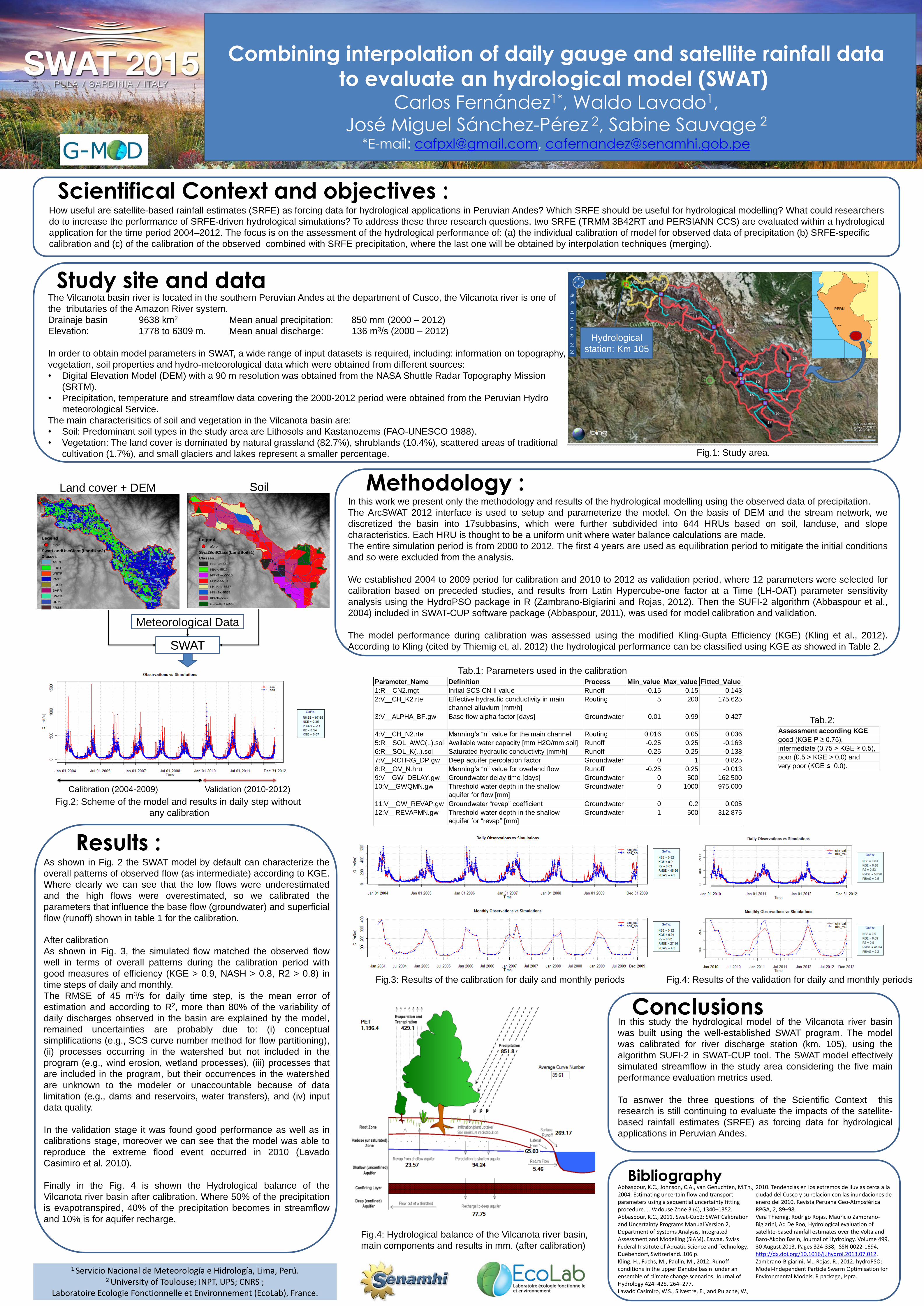
Fig.3: Results of the calibration for daily and monthly periods

Fig.4: Hydrological balance of the Vilcanota river basin,

main components and results in mm. (after calibration)

As shown in Fig. 2 the SWAT model by default can characterize the

overall patterns of observed flow (as intermediate) according to KGE.

Where clearly we can see that the low flows were underestimated

and the high flows were overestimated, so we calibrated the

parameters that influence the base flow (groundwater) and superficial

flow (runoff) shown in table 1 for the calibration.

In this study the hydrological model of the Vilcanota river basin

was built using the well-established SWAT program. The model

was calibrated for river discharge station (km. 105), using the

algorithm SUFI-2 in SWAT-CUP tool. The SWAT model effectively

simulated streamflow in the study area considering the five main

performance evaluation metrics used.

To asnwer the three questions of the Scientific Context this

research is still continuing to evaluate the impacts of the satellite-

based rainfall estimates (SRFE) as forcing data for hydrological

applications in Peruvian Andes.

Assessment according KGE

good (KGE P ≥ 0.75),

intermediate (0.75 > KGE ≥ 0.5),

poor (0.5 > KGE > 0.0) and

very poor (KGE ≤ 0.0).

Tab.2:

Parameter_Name Definition Process Min_value Max_value Fitted_Value

1:R__CN2.mgt Initial SCS CN II value Runoff -0.15 0.15 0.143

2:V__CH_K2.rte Effective hydraulic conductivity in main

channel alluvium [mm/h]

Routing 5 200 175.625

3:V__ALPHA_BF.gw Base flow alpha factor [days] Groundwater 0.01 0.99 0.427

4:V__CH_N2.rte Manning’s “n” value for the main channel Routing 0.016 0.05 0.036

5:R__SOL_AWC(..).sol Available water capacity [mm H2O/mm soil] Runoff -0.25 0.25 -0.163

6:R__SOL_K(..).sol Saturated hydraulic conductivity [mm/h] Runoff -0.25 0.25 -0.138

7:V__RCHRG_DP.gw Deep aquifer percolation factor Groundwater 0 1 0.825

8:R__OV_N.hru Manning’s “n” value for overland flow Runoff -0.25 0.25 -0.013

9:V__GW_DELAY.gw Groundwater delay time [days] Groundwater 0 500 162.500

10:V__GWQMN.gw Threshold water depth in the shallow

aquifer for flow [mm]

Groundwater 0 1000 975.000

11:V__GW_REVAP.gw Groundwater “revap” coefficient Groundwater 0 0.2 0.005

12:V__REVAPMN.gw Threshold water depth in the shallow

aquifer for “revap” [mm]

Groundwater 1 500 312.875

After calibration

As shown in Fig. 3, the simulated flow matched the observed flow

well in terms of overall patterns during the calibration period with

good measures of efficiency (KGE > 0.9, NASH > 0.8, R2 > 0.8) in

time steps of daily and monthly.

The RMSE of 45 m3/s for daily time step, is the mean error of

estimation and according to R2, more than 80% of the variability of

daily discharges observed in the basin are explained by the model,

remained uncertainties are probably due to: (i) conceptual

simplifications (e.g., SCS curve number method for flow partitioning),

(ii) processes occurring in the watershed but not included in the

program (e.g., wind erosion, wetland processes), (iii) processes that

are included in the program, but their occurrences in the watershed

are unknown to the modeler or unaccountable because of data

limitation (e.g., dams and reservoirs, water transfers), and (iv) input

data quality.

In the validation stage it was found good performance as well as in

calibrations stage, moreover we can see that the model was able to

reproduce the extreme flood event occurred in 2010 (Lavado

Casimiro et al. 2010).

Finally in the Fig. 4 is shown the Hydrological balance of the

Vilcanota river basin after calibration. Where 50% of the precipitation

is evapotranspired, 40% of the precipitation becomes in streamflow

and 10% is for aquifer recharge.

Fig.1: Study area.

Abbaspour, K.C., Johnson, C.A., van Genuchten, M.Th., 2004. Estimating uncertain flow and transport parameters using a sequential uncertainty fitting procedure. J. Vadouse Zone 3 (4), 1340–1352. Abbaspour, K.C., 2011. Swat-Cup2: SWAT Calibration and Uncertainty Programs Manual Version 2, Department of Systems Analysis, Integrated Assessment and Modelling (SIAM), Eawag. Swiss Federal Institute of Aquatic Science and Technology, Duebendorf, Switzerland. 106 p. Kling, H., Fuchs, M., Paulin, M., 2012. Runoff conditions in the upper Danube basin under an ensemble of climate change scenarios. Journal of Hydrology 424–425, 264–277. Lavado Casimiro, W.S., Silvestre, E., and Pulache, W.,

2010. Tendencias en los extremos de lluvias cerca a la ciudad del Cusco y su relación con las inundaciones de enero del 2010. Revista Peruana Geo-Atmosférica RPGA, 2, 89–98. Vera Thiemig, Rodrigo Rojas, Mauricio Zambrano-Bigiarini, Ad De Roo, Hydrological evaluation of satellite-based rainfall estimates over the Volta and Baro-Akobo Basin, Journal of Hydrology, Volume 499, 30 August 2013, Pages 324-338, ISSN 0022-1694, http://dx.doi.org/10.1016/j.jhydrol.2013.07.012. Zambrano-Bigiarini, M., Rojas, R., 2012. hydroPSO: Model-Independent Particle Swarm Optimisation for Environmental Models, R package, Ispra.

Fig.4: Results of the validation for daily and monthly periods

Bibliography

Hydrological

station: Km 105