COMBINING INDEPENDENT P-VALUES

BYt

F. W. SCHOLZ

TECHNICAL REPORT NO. 11

SEPTEMBER 1981

DEPARTMENT OF STATISTICSUNIVERSITY OF WASHINGTONSEATTLE) WASHINGTON 98195

i or Sta s cal Anal t wian A sociate ~rnTOC

Statistics at iversi

<: ect ca 6-.J

6 15 6

ABSTRACT

In combining P-values P1, •.. , Pk of k independent tests of hypothesis we findthat the combining statistics of several proposals are of the form T(h =

2:h(Pi)' where h is some nonincreasing function on (0,1), the joint hypothesisbeing rejected when T(h) is too large. We propose to let the P-values themselveschoose the "proper" function h by taking that h (suitably standar-d i zed) which

yields the largest value of T(h) which we denote by Sk' It is shown that Sk isquite easily computed. Its null distribution is derived for k = 2, 3 and

simulated for k =4, ... , 10. A limited power comparison between S2 and Fisher'stest is presented.

P-values, rical dist bu on on,acen i ator al

O. Introduction

Although Fisher's method is certainly the most popular for combining P-values of

independent statistical tests, other proposals, some recent and others not so

recent, have been put forward. For reviews and references on this subject see

Birnbaum (1954), Oosterhoff (1969), Koziol and Perlman (1978), Mudholkar and

George (1979).

It appears that many of these proposals combine the P-values P1, ... , Pk through

a statistic of the following general form:

where h is some decreasing function defined on the interval (0,1). The joint

hypothesis is then rejected if T(h) is too large. As illustration we mention a

few forms for h:

i) h(x) = -2 log x (Fisher, 1932)

ii) h(x) = _<:>-1(x) (Liptak, 1958), here <:>-1 is the inverse of the standard

normal distribution function.

iii) h(x) = -log(x/(l-x)) Mudholkar and Georqe (1979)

Even Tippet s 1931 combining statistics min(P1' •.. , Pk) may in a limiti

sense be subsumed in this wide class of test statistics T(h) as was pointed

to us by M. Perlman; namely consider hr(x) = x-r r > 0 and instead of T(hr).consider T(hr)l/r with r-oo to obtain the reciprocal of Tippet's statistic.

Thus we have a fairly wide class {T(h): h +} of combining test statistics and

each member of this class will yield a most powerful test against some particular

alternative, cf Birnbaum (1954). These alternatives may be quite obscure for

each individual T(h) and certainly are not the main motivation for choosing one

form of T(h) over another. If we did know the alternatives quite specifically we

could deal with the problem via the Neyman Pearson theory. Often, however, the

alternative is specified only vaguely, i.e. one or more of the P-values will te~d

to be stochastically small. We propose to let the P-values "choose the proper"

score function h, namely by selecting that h for which T(h) yields the most

extreme value. For this to be meaningful requires that the functions h be

standardized appropriately, aside from being nonincreasing. This proposal is

nothing but an appl ication of Roy's (1953) union intersection principle to a

nonparametric setting and was inspired by a similar proposal of Behnen (1975) in

the case of two sample linear rank statistics.

Section 1 defines the new combining statistic in detail and presents alternate

f'orms which are amenable to computation. Section 2 examines the null df st r i-

bution of the test statistic, and Section 3 gives a limited examination of its

power behavior in comparison to Fisher's test.

1. Derivation the Test Statistic and its Computation

let H be the class of all real-va ued functions h defined on the interva

es:

i) h is nonincreasing on (Ot1)

.. \11}

1

Jh(x)dx = 0 t and iii)o

Given the observed P-values PIt .•• t Pk from k independent statistical tests,

define the following combination statistic:

(1.1 )

The statistic Sk given in the form (1.1) is not amenable to computation.

Fortunately it turns out that Sk may be computed quite easily once we give its

alternative equivalent representation. To do so we first introduce some nota-

tion.

Let Fk(·) be the empirical cumulative distribution function of PI' ..• , Pk and1\

let Fk(·) be the smallest concave majorant to Fk(·) on the interval (0,1).1\ 1\

Fur-ther, let f k(· r be the left continuous density of Fk(.). The following

proposition represents Sk in a form which may easily be computed as we will

elaborate later.

Proposition 1: Sk' k (J (fk (Xl- l l2dX) Is • :k Ilfk-1112

o

1\Proof: Since Fk is stochastically sma ler than Fk, we have for nonincreasi

(cf. Lehmann 1959

k<

1\

is constant between verteces where Fk

For h E H we further have by the Cauchy Schwarz inequality:

fl.3

* 1\ 1\Note that h (x}: = (fk(x)-1)/llfk-1112 E H and that we have equality in 0.3

* *h(x) = h (x) almost surely. Since h

*touches Fk, one easily sees, taking into account the left continuity of h , that

(1. 4)

Thus (1.2) - (1.4) imply the desired result.

This simple proof of Proposition 1 is, in major parts, due to Piet ~roeneboom and

replaces our earlier, lengthier version which consisted of a modification of

Behnen's argument. Of course Behnen's proof may be shortened similarly. Having

obtained a much more manageable form for Sk' let us give another representation

which outlines a computational algorithm.

i = 1, ... , k be some weights.

the first k(p = 0) i = 1\ 0 ' ••• , k

First denote by c, : p('\-Pr' , \1,0 1; ,1-.;.)

spacings of the ordered Pi and let di,o = 1,

If the c;,o are monotonically increasing then

I

k 2k2 ff2 x dx = C i ,0 where ko = k.

0 = l

If the ci,o are not monotonically increasing, we smooth them out by the following

Pool-Adjacent-Violator algorithm (cf. Barlow et al. 1972): If after the r t h step

in the algorithm we still have

di r, <ci r,

set

for j =1, ••. , i-1

c i , r+1 = c," r + ci+1 r ' di r+1, , , = di r + di +1 r, ,

= k -1.r

for j = ; + 1, .", kr-1

We repeat this process until we finally have

for some s ~ o.

One easily s~es that di,s/{koci,s) represents the slope of the it h

linear segment1\

of Fk, Hence

where

ks 2Rk = ~

di,sG:l ci,s

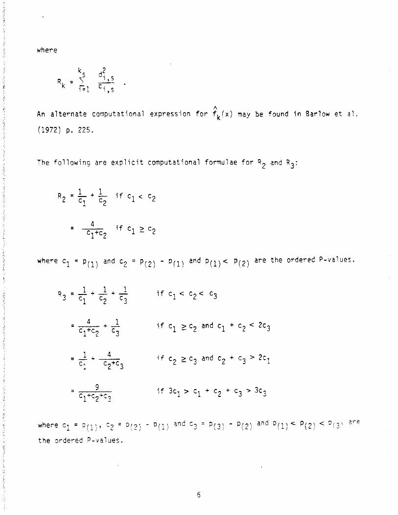
1\An alternate computational expression for fk(x) may be found in Barlow et al.

(1972) p. 225.

The following are explicit computational formulae for R2 and R3:

=

where c1 = P(1) and c2 = P(2) - P(1) and P(1)< P(2) are the ordered P-values.

=

where Cl = PI)' c2 = P 2) - P 1 and c3 = P 3 - P 2 and PI) < P(2 < 0 3

the ordered P-values.

are

2. The Distribution of Sk Under the Hypothesis

Under the hypothesis the o-values PI' ... , Pk are distributed uniformly on the

interval (0,1). The first k spacings Ci = p(i) - P(i-l) (p(o)= 0) i = 1, •.. , k

are distributed uniformly over the simplex

kc. > 0 'ri., L c" < I}, , i=l

(cf. Pyke i965).

From this one may derive expressions for P(Rk $ r) by tedious but straightforward

integration. The resulting expressions for k = 2 and k =3 are given below, the

latter could not be reduced beyond its integral form. For k > 3 one encounters

higher dimensional integrals whose computation does not appear feasible.

k = 2: P(RZ s r) • ~ (1 0 (~n + Go}) VI 0 ~(2.1)

- 22 log (~ - 1 + 7VI - ~ ) for r ~ 4

r

k = 3:

+ a(r)64r3

1r/2

f..1r/2

(r+3-a(r)S;n(x))2cOS(X)(2b (x)(1+b2 XIr r

(2.2)

where a(r) = ((r-9)(r-l))~

and b(r) : cos(x)(cos 2(x) + 8((r-3)a(r)-2 + sin(x) a(r)-l)-~.

The trigonometric terms were introduced by a change of variable in order to

facilitate a more stable numerical quadrature. The distributions of ~2 and R3

are extremely longtailed. Simulations show that the same holds also for Rk ,

k >3. We therefore chose to tabulate the distribution function of a particular

transform of Rk• This transform was suggested by the asymptotic distribution of

Rk (Groeneboom and Pyke (1981), Groeneboom (1981)), namely

S~ - k log k L= _N(O,l)

k J3 log kas k- 00.

One easily sees however, that this convergence is entremely slow. Since Sk ? 0

one finds that the lowest value of Lk1 becomes -2(-3) when k =1.63 105 (k = 5.32

1011).

An alternate limit law is easily derived from the previous one:

Lk2 = 2(Sk - Jk log k )1 j3k LN(O,l) as k -00.

L . h b ++k2 1S muc" . e ....er aved an Lk1. For example, the lowest value

reaches -2 -3) already for k =20 k =854). However simulations for k = 50 s

that the distributions of Lk2 is still somewhat skewed with a heavy right tail.

The logarithmic transform of Sk yields the followinq limit law

Uk = 2"yl 09 k (log \ - {l09(k log k)) ~N(O,l)3

as k- 00.

We found that the distribution of Uk' k = 2, ..• , 10 is quite symmetric but still

shows somewhat heavy tails. We chose to tabulate the distribution function of Uk

partly because of the compact tables that resulted. Table 1 gives the cumulative

distribution function for U3 which was computed by adaptive Romberg quadrature.

Table 2 gives the simulated cumulative distribution functions for Uk' k =4, ..• ,

10, each based on 20,000 replications. The simulations were performed on a PDP

11/45 using the portable random number generator given by Schrage (1979).

3.0 The Power of the S2 Test

As far as the power of the Sk test is concerned, we can only offer some limited

results for k =2. In order to gain intuitive insight into the power behavior of

the S2 test , it is of interest to study the rejection region of the S2 test in

the unit square. This rejection region R is the union of the following three

sets:

where

9

f 2. u I u U

Wl th g(u) = 7 - V7+- t .

The parameter t regulates the size of the test. For t =20 the rejection region

R is depicted in Figure 1. The shape of R is certainly intriguing in that it

tends to make a special effort to reject when both P-values are moderately small.

The acceptance region is not convex which renders the $2 test inadmissible if the

P-values arise from an exponential family testing problem (Birnbaum 1959). This

negative aspect of the $2 test should however be viewed in its proper perspec­

tive. The $2 test arose out of a nonparametric setting whereas the alternatives

in an exponential family testing problem appear to be rather narrow.

Figure 2 compares the rejection region of the $2 test with that of Fisher's test

for significance levels a =.1 and a = .05. We only show the part of the

rejection region that lies below the main diagonal, the other part being obtained

by reflection around it. Also note that abscissa and ordinate have different

scales. For a = .1 the boundary curves for the rejection regions cross each

other four times whereas for a = .05 there are only two crossings. Note that the

S2 test is much more prone to reject than Fisher's test in situations where one

of the P-va ues is very large and the other is small. This feature is also

brought out in the fol owing comparison. For each pair of P-values

which are to be combined, we can compute the P-value Ps of the $2 test and the D.

Actual power calculations are quite difficult in general, however for specific

simple alternatives they may be carried out. These alternatives are as follows:

PI has density 9ab(Pl) and P2 has density gcd(P2) where

with

o < u < 1, 0 s v s 1-a.

The power calculations for either test are straightforward but tedious and we

will not give the resulting formulae, but instead present some numerical results

in tables 3 and 4. Table 3 presents power results under the alternative that

both P-values have the same distribution (a =c, b = d). Table 4 presents power

results under the alternative that P1 - gab and P2 is uniform. We observe that

the S2 test outperforms Fisher's test whenever at least one of the P-values is

distributed very close to zero and Fisher's test performs better otherwise.

Acknowledgements: I would like to thank Professors Piet Groeneboom and Ron Pyke

for sharing their asymptotoic results with me and f)r. Stuart Anderson for

teaching me some things in numerical analysis.

TABLE 1

CUMULATIVE DISTRIBUTION FUNCTION OF U

FOR SAMPLE SIZE H=3

.0 .1 .2 .3 .4 .5 .6 .7 .8 .9

-6 0.00002 0.00002 0.00001 0.00001 0.00001 0.00001 0.00001 0.00001 0.00000 0.00000

-5 0.00010 0.00008 0.00007 0.00006 0.00005 0.00004 0.00004 0.00003 0.00003 0.00002

-4 0.00051 0.00043 0.00036 0.00031 0.00026 0.00022 0.00019 0.00016 0.00013 0.00011

-3 0.00273 0.00230 0.00194 0.00164 0.00139 0.00117 0.00099 0.00084 0.00071 0.00060

-2 0.01504 0.01267 0.01067 0.00899 0.00757 0.00638 0.00538 0.00454 0.00383 0.00323

-1 0.08274 0.07002 0.05917 0.04995 0.04213 0.03550 0.02991 0.02519 0.02121 0.01iB6

0 0.36424 0.32174 0.28220 0.24592 0.21308 0.18368 0.15763 0.13476 0.11483 0.09758

.0 .1 .2 .3 .4 .5 .6 .7 .8 .9

0 0.36424 0.40920 0.45600 0.50385 0.55187 0.59917 0.64487 0.68822 0.72859 0.76555

1 0.79884 0.82841 0.85433 0.87680 0.89611 0.91258 0.92653 0.93831 0.94822 0.9565:-

2 0.96350 0.96934 0.97423 0.97833 0.98176 0.98464 0.98705 0.98908 0.99079 0.99222

3 0.99343 0.99445 0.99531 0.99605 0.99666 0.99717 0.99761 0.99797 0.99828 0.99855

4 0.99877 0.99896 0.99912 0.99925 0.99937 0.99946 0.99954 0.99961 0.99967 0.99972

5 0.99976 0.99980 0.99983 0.99986 0.99988 0.99990 0.99991 0.99993 0.99994 0.99995

6 0.99995 0.99996 0.99997 0.99997 0.99998 0.99998 0.99998 0.99999 0.99999 0.99999

TABLE 2

E:1?IRICAL CL;~iUL;';IVE DISiRItUTICt{ FUHc;ION OF U

FOR SA~PLE SIZE N B~SED ON 200GO REPLICATIGHS

x

-4.9-4.8-4.7-4.6-4.5-4.4-4.3-4.2-4.1-4.0-3.9-3.8-3.7-3.6-3.5-3.4-3.3-3.2-3.1-3.0-2.9-2.8-2.7-2.6-2.5-2.4-2.3-2.2-2.1-2.0-1. 9-1.8-1.7-1.6-1.5-1.4-1.3-1.2-1.1-1.0-0.9-0.8-0.7-0.6-0.5-0.4-0.3-0.2-G.lo. a

0.00050.00050.00050.00070.000030.000030.00090.00110.00120.00120.00160.00190.00210.00230.00240.00280.00320.00370.00430.00490.00570.00650.00770.00380.01030.01170.01350.01580.01890.02250.02600.02<;80.03450.04060.04720.05390.06580.07650.OgS50.10380.12070.13840.15910.18380.2114­o.2414­0.27180.30790.3462O.3t52

1\=5

0.00040.00040.00050.00050.00060.00070.00070.00100.00130.00150.0019o . 0-0210.00220.00230.00260.00290.00340.00380.00440.00570.00630.00710.00830.01020.01190.01420.01630.01890.02180.02570.03010.03540.04180.04870.05610.06530.07480.OS650.1005o .115S0.13390.15460.17600.20110.22960.25930.29290.32740.36560.4060

"=6

0.00050.00060.00060.00070.00090.00100.00120.00150.00160.00190.00210.00220.00260.00300.00350.00420.00480.00530.00610.00690.00790.00910.01060.01240.01440.01680.01920.02240.02630.03010.03490.03920.04530.05290.06150.07030.08150.09310.106S0.12130.13830.15960.18320.20680.23440.26270.29570.33e80.36630.4056

N=7

0.00070.00070.00090.00090.00120.00130.00160.00190.00200.00230.00270.00300.00350.00400.00430.00510.00580.00660.00790.00900.01000.01100.01310.01490.01680.02010.02280.02640.03090.03460.03950.04480.05050.05810.06730.07730.DS870.10080.11520.13060.15060.16890.1924o .21770.24620.277 90.31010.34500.38320.4217

0.00090.00100.0010O.OOlC0.00120.00140.0016O.OOB0.00230.00280.00320.00340.00400.00480.00530.00580.00660.00700.00790.00880.01020.01180.01340.01550.01820.02080.02410.02720.03050.03510.04020.04600.05310.06060.07060.07990.09050.1018o .115S0.13180.15000.16960.19100.21910.2471o . 277 00.30970.34590.37970.4158

H=9

0.0:ll10.00120.00160.001~

0.00180.00210.00240.00260.00290.00320.00360.00400.00460.00530.00580.00670.00740.00S40.00940.01080.01180.01360.01510.01730.01950.02210.02540.02SS0.03240.03690.04230.04840.05530.06300.07360.08350.09460.10800.12600.14250.1618O. IS 130.202S0.22(';70.25750.28770.31890.35190.38690.4245

H=10

0.00100.00120.00150.00160.00130.00200.00210.00250.00260.00300.00350.00390.00450.00490.00540.OC610.00680.00780.00870.00990.010130.0123O. Ul420.01570.01820.02060.02350.02670.03050.03520.04090.04710.05340.06150.Oil30.08150.09320.10600.12240.13970.15860.17890.20270.22790.25840.28850.32110.35550.39270.4292

TABLE 2 (Continued)

EMPIRICAL CUMUlATIV~ DISTRIBUTION FU~CTION OF U

FOR SAMPLE SIZE N BASED ON 20000 ~EPLICATIONS

0.1o.20.30.40.50.6o.70.80.91.01.11.21.31.41.51.61.71.81.92.02.12.22.32.42.52.62.72.82.93.03.13.23.33.43.53.63.73.83.94.04.14.24.34.44.54.64.74.84.95.0

H=4

0.4Z870.47300.51940.56310.60810.65280.69350.72970.76420.79470.82100.34610.86870.8~75

0.90470.91830.93160.94240.95190.95910.96540.97050.97630.97930.98170.98410.98610.98820.98960.99100.99190.99320.99380.99500.99560.9%10.99630.99680.99730.99730.99820.99860.99880.99390.99890.99920.99930.99940.9'1950.9996

1'1=5

0.44630.48730.52920.57350.61310.65110.68970.72390.75810.78S70.81560.83850.S6160.8S120.89340.91l80.92440.93570.94570.95420.96050.96570.97020.97440.97800.98060.9836o. 985&0.98740.98930.9909O. 99220.99370.99460.99520.99570.99620.99650.99720.99740.99760.99790.99810.99320.99&50.99870.99380.99910.99920.9993

0.44710.48810.53060.56980.60890.64S40.68770.72360.7563o.13600.S1l70.83850.85920.87810.89370.90710.91980.93090.94020.94810.95490.96000.96560.97070.97420.97720.98030.98270.98460.98640.98800.98950.9905'0.99170.99260.99370.99440.99520.99580.99640.99670.99680.99730.99770,99790.99310.99830.99840.~985

0.9987

1'1=7

0.46100.50000.54090.58150.62060.65680.69240.72600.75900.78930.81530.84040.85970.87790.89500.90920.92190.93250.94130.94900.95660.96250.96760.97180.9752o. 97840.98110.98390.98560.98740.98860.99010.99150.99240.99320.99420.99470.99550.99620.99660.99700.99720.99740.99790.99810.99520.9(;830.99~6

0.9'1S90.9,t.9

0.45550.49590.53480.57470.b1430.65120.68910.72310.75650.78440.81020.8351o.85690.87740.89410.90720.91S70.92980.93930.94680.95390.95960.96500.96890.97250.97590.97910.98160.98400.98590.98750.98950.99050.99170.99260.99340.99420.99470.99540.99600.99640.99670.99700.99740.99770.9979O.99Z20.9983O.9C;S50.9936

0.46370.50280.54550.58300.62170.65750.69310.72570.75710.18570.81230.83550.85700.87500.89210.90550.91650.92660.93570.94430.95060.95700.96260.96720.97140.97450.97760.98050.98310.98500.98690.98850.98990.99100.99180.99260.99340.99420.99470.99530.99580.99650.99700.99730,99770.9979O.9C;S10.<;9S30.99870.9953

H=10

0.46730.50670.54310.58280.62290.66080.69460.72810.75990.78780.81250.83780.85620.87560.89160.90500.91830.92920.93750.94590.95260.95930.96360.96780.97200.97510.97770.98040.98260.98470.9863o. 9S 770.98890.9904O.99~5

0.99250.99320.9940O.9<,l460.99530.99560.99600.99650.9';72o. 9 <17:·0.99790.9981a.9985C.C;gS7O.9C;90

b .05

a = .02 F .1248

$2 .1445

a = .05 F .0954

$2 .0987

a = .08 F .0837

$2 .0839

a = .10 F .0791

$2 .0778

a = .20 F .0672

$2 .0640

a = .30 F .0622

$2 .0593

a = .05

.1

.1968

.2340

.1412

.1475

.1194

.1198

.1109

.1076

.0862

.0785

.0756

.0689

TABLE 3

a = c

.2

.3323

.3982

.2345

.2456

.1970

.1977

.1827

.1727

.1300

.1094

.1056

.0889

b = d

.3

.4565

.5426

.3299

.3443

.2829

.2839

.2655

.2454

.1812

.1426

.1401

.1101

.5

.6708

.7721

.5268

.5434

.4796

.4806

.4637

.4136

.3060

.2160

.2225

.1558

.8

.9072

.9680

.8376

.8465

.8364

.8369

.8430

.7225

.5495

.3436

.9

.9633

.9937

.9454

.9487

.9719

.9720

.9912

.8407

Power of Fisher's (F) test and the S2 test when both P-val ues have the same

density gab x).

15

TABLE 4

a = .05 d = a

S2 .0985

S2 .0743

S2 .0664

S2 .0634

$2 .0568

$2 . 0546

b

a = .02 F

a = •as F

a = .08 F

a = .10 F

a = .20 F

a = .30 F

.05

.0881

.0726

.0663

.0639

.0581

.0558

.1

.1263

.1469

.0951

.0986

.0826

.0829

.0777

.0769

.0662·

.0637

.0617

.0592

.2

.2025

.2439

.1402

.1472

.1153

.1157

.1055

.1038

.0825

. 0773 .

.0734

.0683

.3

.2788

.3408

.1853

.1958

.1479

.1486

.1332

.1307

.0987

.0910

.0850

.0775

.5

.4313

.5347

.2755

.2930

.2131

.2143

.1886

.1845

.1312

.1184

.1084

.0959

.8

.6600

.8255

.4108

.4388

.3110

.3128

.2718

.2651

.1800

.1594

.9

.7363

.9224

.4559

.4875

.3436

.3457

.2996

.2920

Power of Fis 's F test the S2 test when PI has

uniformly distributed.

a , V

.8

.6

. 4

.2

-

.

-liZ

. --III

I R)II I I

o .2 .4 .6 .8 1.0

Figure 1. Rejection Region of the $2 Test

• It.

--- ----- Fisher's test

--- 52 test

- -- - .......

//

//

I'a • .1/ ',,(

/~t12"""" ----a • .05 • - - - - - - - - - - - _ _ _ - - - . - --------- ------ .....

.28

.20

.24

.16

.08

.12

.04

•." . 2 .3 .4 .5 .6 .7 .8 .9 1.0

Figure 2. Comparison of Rejection Regions

1.0~

~,,.9 ,

Ps < PF~,

~,~

.8 ,,,,,.7 PF < Ps

,~

i,,,

Ps < PF,

.6,,,,,

~

.5 ,

,.4

,,,,

,.3 ,

.2PF < Ps

.1 ,Ps < PF,,,

0,

.1 .2 .3 .4 .5 .6 .7 .8 .9 1.0

Figure 3. Comparison of Ps and PF

References

Barlow, R.E., Bartholomew, D.J., Bremner, J.M. and Brunk, H.O. (1972),Statistical Inference Under Order Restrictions, John Wiley &Sons, London, ~ew

York.

Behnen, K. (1975) "The Randles-Hogg Test and an Alternative Proposal," Corrrn. inStat. 4(3), 203-238.

Birnbaum, A. (1954), "Combining Independent Tests of Significance," J. AmericanStatist. Assoc., 49, 559-575.

Fisher, R.A. (1932), Statistical Methods for Research Workers, Oliver and Boyd,Edinburgh, London, 4th ed.

Groeneboom P. and Pyke R. (1981), "Asymptotic Normality of Statistics Based onConvex Minorants of Empirical Distribution Functions," Technical Report No.5,Department of Statistics, University of Washington, Seattle.

Groeneboom, P. (1981), "The Concave Majorant of Brownian Motion," TechnicalReport No.6, Department of Statistics, University of Washington, Seattle.

KOZiol, J.A. and Perlman, M.D. (1978), "Combining Independent Chi-Squared

Tests," J. American Statist. Assoc., 73, 753-763.

Lehmann, LL. (1959), Testing Statistical Hypotheses, John Wiley & Sons, New

York, London.

liptak, T. (1958), "On the Combination of Independent Tests," Magyar Tud. Akad.

Mat. Kutato Int. Kozl. 3, 171-197.

Mudholkar, G. S. and George, E. O. 1979, "The Logit Statistic for Comb inProbabilities - an Overview," OptimiZing Methods in Statistics, Rustagi

Academic Press.

9

Oosterhoff, J. (1969), Combination of One-~ided Statistical Tests, MathematischCentrum, Amsterdam.

Pyke, R. (1965), "Spacings," J. R. ~tatist. Soc. B 27, 395-436.

Roy, S. N. (1953), "On a Heuristic Method of Test Construction and its Use inMultivariate Analysis," Ann. Math. Stat. 24, 220-238.

Schrage, L. (1979), "A More Portable Fortran Random Number Generator," ArM Trans.

Math. Software, S, 132-138.

Tippet, L. H. C. (1931), The Method of Statistics, First edition, Williams and

Norgate, London.