Available at: http://hdl.handle.net/2078.1/158816 [Downloaded 2022/03/18 at 01:48:12 ]

"Quantification of topsoil organic carbon in Europe : a statistical approachcombining harmonised soil and land cover point data with spatial layers"

de Brogniez, Delphine

ABSTRACT

Soil organic carbon (OC) has been recognised as important for soil quality, soil resilience to degradationprocesses, but also as playing a major role in providing ecosystem services and in mitigating climatechange. In this context, there is an urgent need for up-to-date data on the status of soil organic carbon.From local to global scale, the comprehensive assessment of soil OC faces several challenges relatedto soil OC spatial and temporal variability, to the lack of standard soil sampling and analytical protocolsand to the absence of geo-referencing of most legacy data. The aim of this thesis was to produce themost up-to-date representation of the spatial distribution of topsoil OC content for 25 Member States ofthe European Union and to estimate the total amount of OC in the upper layer of the soils (0-20cm) inthese same countries. To do so, ca. 20,000 OC measurements and land cover observations from the firstharmonised topsoil database at European scale, the so-called LUCAS survey, were used. Specifically inthis thesis, (i) a spatial database was built, consisting of soil data and environmental covariates relevantto the study of OC levels in European soils; (ii) the spatial distribution of topsoil OC content was predictedand represented by applying two different digital soil mapping techniques. The uncertainties associatedto the predictions were also produced; (iii) a method for the quantification of topsoil OC stocks in Europewas proposed and applied. The results confirmed the difficulty to map and account for OC levels in soils,due to its high spatial...

CITE THIS VERSION

de Brogniez, Delphine. Quantification of topsoil organic carbon in Europe : a statistical approach combiningharmonised soil and land cover point data with spatial layers.  Prom. : van Wesemael, Bas ; Montanarella,Luca http://hdl.handle.net/2078.1/158816

Le dépôt institutionnel DIAL est destiné au dépôtet à la diffusion de documents scientifiquesémanant des membres de l'UCLouvain. Touteutilisation de ce document à des fins lucrativesou commerciales est strictement interdite.L'utilisateur s'engage à respecter les droitsd'auteur liés à ce document, principalement ledroit à l'intégrité de l'œuvre et le droit à lapaternité. La politique complète de copyright estdisponible sur la page Copyright policy

DIAL is an institutional repository for the depositand dissemination of scientific documents fromUCLouvain members. Usage of this documentfor profit or commercial purposes is striclyprohibited. User agrees to respect copyrightabout this document, mainly text integrity andsource mention. Full content of copyright policyis available at Copyright policy

Quantification of topsoil organic

carbon in Europe

A statistical approach combining harmonised soil and land cover

point data with spatial layers

Delphine de Brogniez

Thèse présentée en vue de l’obtention du grade de

Docteur en Sciences

Université catholique de Louvain

Mars 2015

Composition du jury de thèse

Présidente du jury

Prof. Marie-Laurence De Keersmaecker (Université catholique de Louvain,

Belgique)

Promoteurs

Prof. Bas van Wesemael (Université catholique de Louvain, Belgique)

Dr. Luca Montanarella (European Commission, Italy)

Membres

Dr. Robert Jones (Cranfield University, United Kingdom)

Dr. Antoine Stevens (Université catholique de Louvain, Belgique)

Prof. Christian Walter (Institut National de Recherche Agronomique, France)

i

ACKNOWLEDGEMENTS

Cette thèse de doctorat est l’aboutissement de trois années de dur labeur. Je

prends ici la plume pour remercier ceux qui ont collaboré à son élaboration.

Tout d’abord, je tiens à remercier mon promoteur, Bas van Wesemael, pour

son soutien tout au long du projet. Réaliser une thèse à distance est un défi de

taille que nous sommes parvenus à relever ensemble. Non seulement Bas m’a

guidée durant ces trois années mais il m’a surtout beaucoup appris. Avec son

incroyable mémoire, et ayant constamment en tête le fil rouge de mon projet, il

m’a permis de rester sur les rails, m’offrant néanmoins le « luxe » d’explorer les

pistes qui m’intéressaient. Cher Bas, merci pour ta confiance, ta constance dans

le suivi de mon projet, ton éternelle bonne humeur et pour les blagues cachées

en marge de pages! Furthermore, I would like to thank my other supervisor,

Luca Montanarella, for convincing me to enroll as a PhD student at the first

place and for giving me the opportunity to live a wonderful “European

experience”. Working at the JRC, within a team of passionate and enthusiastic

soil scientists, was probably the best I could have dreamt of for the beginning

of my career. You allowed me to travel around the world (literally) and to be

part of the global soil science community – thanks for your trust and constant

encouragements.

My sincere gratefulness goes to Bob Jones, without whom this whole story

would have never started. That day I knocked the door of your office in

Cranfield undoubtedly marked the start of a wonderful European-Soil-journey.

Thank you for always being there, for picking up the phone even when on the

top of a mountain, for unearthing precious documents from the NSRI archives

ii

and for spending hours thoroughly adding “les mots justes”… It has been a

privilege to work by your side and to benefit from your experience!

Un tout grand merci à Antoine Stevens pour ses précieux conseils, sa

disponibilité et pour les advanced tutorials de ggplot! Je tiens aussi à remercier

le Professeur Christian Walter pour le vif intérêt qu’il a montré à l’égard de

mon travail et pour ses commentaires qui ont permi d’améliorer la qualité du

manuscrit.

The completion of this thesis would have never been possible without the

support of Cristiano Ballabio. The mix of your thorough knowledge of soil C

and DSM, your pedagogy and infinite patience together with my eagerness to

learn resulted in a fantastic team driven by the same passion for equations and

soil protection! You turned R into a fun experience although I was terrified by

it; this new skill will accompany me in my career, thanks a million for that!

Grazie a te per aver reso questi anni cosi interesssanti… e molto divertenti!

One cannot think of doing a PhD without having friends embarked on the

same boat … I was so lucky to share my excitement when plotting my first

graphs with R, my happiness when obtaining a first decent map, my explosion

of joy when my first article was eventually published but also my nervousness

before the first conference talk, my irritation caused by the tidious peer-review

process, my tiredness during the writing-up of the final manuscript and all my

doubts along the way with Vera, Bettina, Elisabeth, Anouk, Emilie and Aurélie.

There is a light at the end of the tunnel indeed; I was delighted to walk/crawl

through its darkness with you girls! Having friends that are NOT (or not

anymore) embarked on a “PhD boat” is probably even more important to keep

you sane and with your feet on the ground. I wish to thank Ale, Giorgia,

Mélanie & Greg, Joe and Joana in Italy, Laura in Spain, et Nath en Belgique, for

having supported me during the last three years. Your friendship is priceless!

Enfin, je remercie du plus profond de mon cœur, ma famille, pour leur soutien

et leur amour inconditionnel.

iii

TABLE OF CONTENTS

ACKNOWLEDGEMENTS I

LIST OF PUBLICATIONS VII

LIST OF FIGURES IX

LIST OF TABLES XI

LIST OF ABBREVIATIONS XIII

INTRODUCTION 1 GENERAL INTRODUCTION .......................................................................................... 1 PROBLEM STATEMENT ................................................................................................. 2 OBJECTIVES OF THE THESIS ........................................................................................ 4 OUTLINE OF THE THESIS ............................................................................................. 6

CHAPTER 1. SOIL ORGANIC CARBON IN EUROPE 9 1.1. SOIL MAP OF EUROPE ........................................................................................... 9 1.2. THE DECLINE IN SOIL ORGANIC MATTER: A THREAT TO EUROPEAN SOILS ........................................................................................................................................ 11 1.3. SOIL ORGANIC MATTER AND SOIL ORGANIC CARBON ................................. 13 1.4. FIRST MAP OF TOPSOIL ORGANIC CARBON CONTENT FOR EUROPE ......... 16

1.4.1. Pedo-transfer rule ..................................................................................... 16 1.4.2. OCTOP map ............................................................................................. 17

1.5. SOIL ORGANIC CARBON VARIABILITY IN SPACE AND TIME – A NEED FOR MONITORING NETWORKS .......................................................................................... 18

1.5.1. Quantification of OC pools .................................................................... 18 1.5.2. Soil monitoring networks in Europe ..................................................... 20

1.6. THE LUCAS SURVEY ........................................................................................... 23 1.6.1. Topsoil sampling ....................................................................................... 24 1.6.2. Laboratory analysis ................................................................................... 25

1.7. EVOLUTION OF SPATIAL MODELS .................................................................... 28 1.7.1. Soil survey and soil mapping ................................................................... 29 1.7.2. The theory of digital soil mapping ......................................................... 30 1.7.3. Recent OC digital mapping studies ........................................................ 32

iv

CHAPTER 2. LUCAS DATABASE CLEANING AND COLLECTION OF COVARIATES 33 2.1. LUCAS DATABASE CLEANING .......................................................................... 33 2.2. ENVIRONMENTAL COVARIATES ........................................................................ 35

2.2.1. Land cover ................................................................................................. 35 2.2.2. Pre-Quaternary geology ........................................................................... 35 2.2.3. Soil reference group and qualifier .......................................................... 35 2.2.4. Terrain attributes ....................................................................................... 36 2.2.5. Climatic data .............................................................................................. 36 2.2.6. Net primary productivity ......................................................................... 37 2.2.7. Soil texture ................................................................................................. 38 2.2.8. Spatial resolution of the covariates ........................................................ 39

CHAPTER 3. MAPPING TOPSOIL ORGANIC CARBON CONTENT WITH REGRESSION KRIGING 40 3.1. ABSTRACT .............................................................................................................. 40 3.2. INTRODUCTION .................................................................................................... 41 3.3. MATERIALS AND METHODS ............................................................................... 42

3.3.1. Soil Data ..................................................................................................... 42 3.3.2. Environmental Covariates ....................................................................... 42 3.3.3. Spatial Prediction ...................................................................................... 42

3.4. RESULTS AND DISCUSSION ................................................................................ 43 3.4.1. Environmental Covariates Selection and Linear Regression ............. 43 3.4.2. Kriging and Variogram Modelling ......................................................... 45 3.4.3. OC Content Prediction and Model Accuracy ...................................... 47 3.4.4. Comparison with the OCTOP map ...................................................... 51

3.5. CONCLUSIONS ...................................................................................................... 51

CHAPTER 4. MAPPING TOPSOIL ORGANIC CARBON CONTENT BY APPLYING A GENERALISED ADDITIVE MODEL 53 4.1. ABSTRACT........................................................................................................... 53 4.2. INTRODUCTION .................................................................................................... 54 4.3. MATERIALS AND METHODS ............................................................................... 54

4.3.1. Soil data ...................................................................................................... 54 4.3.2. Environmental covariates ........................................................................ 54 4.3.3. OC prediction model................................................................................ 55 4.3.4. Mapping ...................................................................................................... 56

4.4. RESULTS AND DISCUSSION ................................................................................. 57 4.4.1. Data exploratory analysis ......................................................................... 57 4.4.2. OC model ................................................................................................... 62 4.4.3. OC predictions and standard error maps .............................................. 68 4.4.4. Comparison with existing OC map........................................................ 71

4.5. CONCLUSION ........................................................................................................ 75

v

CHAPTER 5. ESTIMATING TOPSOIL ORGANIC CARBON STOCKS IN EUROPE USING GEO-REFERENCED HARMONISED TOPSOIL AND LAND COVER DATA 76 5.1. ABSTRACT .............................................................................................................. 76 5.2. INTRODUCTION .................................................................................................... 77 5.3. MATERIALS AND METHODS ............................................................................... 81

5.3.1. Input data ................................................................................................... 81 5.3.2. Prediction models ..................................................................................... 87 5.3.3. Soil organic carbon stocks ....................................................................... 90

5.4. RESULTS AND DISCUSSION ................................................................................. 94 5.4.1. Models calibration and validation........................................................... 94 5.4.2. Predictions................................................................................................ 101

5.5. CONCLUSION ...................................................................................................... 116

CONCLUSION 121 MAIN FINDINGS ......................................................................................................... 121 LIMITATIONS .............................................................................................................. 125 OUTLOOK ................................................................................................................... 127

REFERENCES 130

APPENDICES 145

vii

LIST OF PUBLICATIONS

de Brogniez, D., Ballabio, C., Stevens, A., Jones, R.J.A., Montanarella, L., van Wesemael, B., 2014. A map of the topsoil organic carbon content of Europe generated by a generalized additive model. European Journal of Soil Science n/a–n/a.

de Brogniez, D., Ballabio, C., van Wesemael, B., Jones, R.J.A., Stevens, A., Montanarella, L., 2014. Topsoil organic carbon map of Europe, in: Hartemink, A.E., McSweeney, K. (Eds.), Soil Carbon, Progress in Soil Science. Springer International Publishing, pp. 393 – 406.

Banwart, S., Black, H., Cai, Z., Gicheru, P., Joosten, H., Victoria, R., Milne, E., Noellemeyer, E., Pascual, U., Nziguheba, G., Vargas, R., Bationo, A., Buschiazzo, D., de Brogniez, D., Melillo, J., Richter, D., Termansen, M., van Noordwijk, M., Goverse, T., Ballabio, C., Bhattacharyya, T., Goldhaber, M., Nikolaidis, N., Zhao, Y., Funk, R., Duffy, C., Pan, G., la Scala, N., Gottschalk, P., Batjes, N., Six, J., van Wesemael, B., Stocking, M., Bampa, F., Bernoux, M., Feller, C., Lemanceau, P., Montanarella, L., 2014. Benefits of soil carbon: report on the outcomes of an international scientific committee on problems of the environment rapid assessment workshop. Carbon Management 5, 185–192.

Montanarella, L., Bampa, F., de Brogniez, D., 2014. Policy Frameworks. In: Banwart, S. A., Noellemeyer, E., Milne, E., (Eds.) Soil Carbon - Science, Management and Policy for multiple benefits. SCOPE Series Volume 71, Wallingford, UK.

de Brogniez, D., Ballabio, C., Stevens, A., Jones, R.J.A., Montanarella, L., van Wesemael, B., 2014. Topsoil organic carbon content of Europe, a new map based on a generalised additive model, in: EGU General Assembly Conference Abstracts, EGU General Assembly Conference Abstracts. p. 7206.

ix

LIST OF FIGURES

Figure 0-1 Chapters of the thesis. ............................................................................... 8 Figure 1-1 Measured organic carbon content at LUCAS topsoil survey (2009)

sampling locations. ............................................................................................. 27 Figure 1-2 Histogram of OC content in LUCAS topsoil samples. ...................... 28 Figure 3-1 Empirical variograms of OC measurements (blue) and regression

residuals (red) with 3,000 km (left) and 150 km (right) cut-off. .................. 46 Figure 3-2 Kriged regression residuals. .................................................................... 47 Figure 3-3 Topsoil organic carbon content estimates. ........................................... 48 Figure 3-4 Cumulative density function of the regression kriging residuals. ..... 49 Figure 3-5 Regression kriging residuals at sampling locations. ............................ 50 Figure 4-1 Histogram and summary descriptive statistics of measured OC

content in calibration (a) and validation (b) sets. ........................................... 58 Figure 4-2 Boxplot of OC content (logarithmic scale) for each land-cover class,

as defined in the LUCAS survey nomenclature. ............................................ 59 Figure 4-3 Scatterplot between measured OC content and covariates in mineral

(a) and organic (b) soils. ..................................................................................... 61 Figure 4-4 QQplot of the calibration residuals. ...................................................... 62 Figure 4-5 Smooth function of temperature as produced by the GAM model. 64 Figure 4-6 Predicted values plotted against observed OC contents in the

validation set. Other countries (a) and Scandinavia (b). ............................... 66 Figure 4-7 Map of predicted topsoil organic carbon content (g kg-1). ................ 69 Figure 4-8 Map of standard error of the OC model predictions (g C kg-1). ....... 71 Figure 4-9 Scatterplot of OC content predictions proposed by Jones et al.

(2005) and by our model in Scandinavia (b) and other countries (a). ........ 73

x

Figure 4-10 Comparison of mean OC content predictions (g kg-1) per land-

cover class, for OCTOP and for the GAM model (this study). ................. 74 Figure 5-1 Methodology for the calculation of OC stocks, with logical flow

indicated by capital letters (A-I). ...................................................................... 85 Figure 5-2 Comparison of the national OC stocks (Gt) at a 0-30 cm depth, as

predicted in the present study and by Hiederer (2010). ............................. 106 Figure 5-3 National OC stocks in t C ha-1. ............................................................ 109 Figure 5-4 National OC stocks in Gt C with bars showing the lower and upper

limit of the 95% standardised confidence interval. ..................................... 110 Figure 5-5 Comparison of the OC stocks (Gt) predictions for a 30 cm depth

made by Lugato et al. (2014) for the agricultural soils of Europe and the

predictions made in this study. ....................................................................... 115

xi

LIST OF TABLES

Table 3-1 Relative importance of the independent variables in the multiple

linear regression model, expressed by the absolute value of the t-statistic.

............................................................................................................................... 44 Table 4-1 Correlation matrix of measured OC content and covariates used in

the regression model. ......................................................................................... 60 Table 4-2 Summary table of the GAM models tested by backward step-wise

removal of the covariates. ................................................................................. 63 Table 4-3 Model accuracy (RMSE, root mean square error, g kg-1) and

normalised root mean squared error (NRMSE, %) calculated for mineral

and organic soils (OC content > 200 g kg-1) and for each LUCAS land-

cover class. ........................................................................................................... 68 Table 5-1 Theoretical confusion matrix, as generated in this study. ................... 89 Table 5-2 Summary table for the goodness-of fit and error of the selected best

prediction models for OC content (in mineral soils). ................................... 95 Table 5-3 Number of samples and summary statistics of measured and

predicted OC content for each soil class*land cover type combination. .. 96 Table 5-4 Selected covariates for every model. ....................................................... 97 Table 5-5 Confusion matrices and performance tests parameters....................... 99 Table 5-6 Summary table presenting OC stocks for the 23 countries of the

study. ................................................................................................................... 104 Table 5-7 Summary table of the OC stocks predictions (Gt) per land cover at

20 cm depth. ...................................................................................................... 113

xiii

LIST OF ABBREVIATIONS

AIC: Akaike Information Criterion

AAT: Annual Accumulated Temperature

BD: Bulk Density

CO2: Carbon dioxide

CORINE: CORdinate INformation on the Environment

DEM: Digital Elevation Model

DG-ENV: European Commission’s Directorate General for the Environment

DG-JRC: European Commission’s Directorate General Joint Research Centre

DSM: Digital Soil Mapping

ENVASSO: Environmental Assessment of Soil for Monitoring

ESDB: European Soil DataBase

ESGDB: European Soil Geographical DataBase

EU: European Union

EVI: Enhanced Vegetation Index

FAO: Food and Agriculture Organisation (of the United Nations)

GAM: Generalised Additive Model

GLM: Generalised Linear Model

LUCAS: Land Use/Cover Area frame Statistical survey

MARS: Monitoring Agriculture with Remote Sensing

MODIS: Moderate Resolution Imaging Spectroradiometer

NASA: National Aeronautics and Space Administration

NDVI: Normalised Difference Vegetation index

NPP: Net Primary Productivity

NRMSE: Normalised Root Mean Squared Error

NUTS: Nomenclature of the Territorial Units for Statistics

xiv

OC: Organic Carbon

OCTOP: map of TOPsoil Organic Carbon in Europe (Jones et al., 2005)

OM: Organic Matter

PESERA: Pan European Soil Erosion Risk Assessment

PTR: Pedo-Transfer Rule

RK: Regression Kriging

RMSE: Root Mean Squared Error

SMU: Soil Mapping Unit

SRTM: Shuttle Radar Topography Mission

STU: Soil Typological Unit

UNESCO: United Nations Educational, Scientific and Cultural Organisation

UNFCCC: United Nations Framework Convention on Climate Change

WRB: World Reference Base

1

INTRODUCTION

GENERAL INTRODUCTION Soil is an exhaustible natural resource and it is non-renewable on a human time

scale. Soil is a complex porous environment, consisting of mineral and organic

particles, interspersed with water and gases. It is home to a myriad of living

organisms, with size ranging from the micro- to the macro scale; it provides the

basis for food, fibre and biomass production; it stores and filters water and

regulates the release of various gases in the atmosphere. As such, soil is

recognised as a major contributor to sustain life on earth.

Historically, soil scientists focussed on understanding the processes responsible

for soil formation and on controlling the factors ensuring productive

agricultural systems (Montanarella et al., 2004). In the late 1980’s, on-going

degradation of soils was widely observed by experts in Europe and the

prevention of irreversible consequences of these processes on the environment

and living organisms became a priority.

Intensive agricultural practices such as the use of heavy machinery; water

management systems (drainage, irrigation); the use of chemical fertilisers and

pesticides; the shortening or ceasation of rotation cycles eventually lead to the

obvious degradation of soils (Oldeman et al., 1990). These degradation

processes translate into soil compaction; soil erosion; salinisation; removal of

soil nutrients; soil contamination and decline in soil biodiversity which in turn

jeopardise soil’s ability to carry out essential functions (Lal, 2010). Man-made

activities such as soil sealing (Huber et al., 2008) or land use change for

agriculture or urban development purposes also greatly affect soil conditions.

2

In particular, there is a growing interest to address the decline in soil organic

matter as the latter directly affects soil fertility and soil resilience to further

degradation. Furthermore, the potential of soils to sequester organic carbon

(which is the principal component of soil organic matter) or to release it as

atmospheric carbon dioxide is of major importance to address the global issue

of climate change. Also, organic carbon is recognised as an essential property

for soils to function properly and to deliver ecosystem services (Banwart et al.,

2014). Through these effects, soil organic carbon has been defined as an

important contributor to soil quality (Doran & Parkin, 1994), as an indicator of

global soil conditions (Koch et al., 2013) and of environmental quality (Ogle &

Paustian, 2005). In this context, soil organic carbon has gained the attention of

policy-makers and has triggered a growing interest in the science community,

over the last two decades.

PROBLEM STATEMENT As soil carbon receives a global recognition of its major role in ensuring key

ecosystem services and in mitigating climate change, the need for up-to-date

data is expanding from field to global scale (McBratney et al., 2003; Sanchez et

al., 2009).

A significant challenge in the assessment of the status of soil organic carbon

(OC) is its high spatial and temporal variability. Moreover, the lack of standard

protocols for soil sampling and for the analysis of OC in soils results in

heterogeneous datasets that prove difficult to be combined for large-scale

assessments. The design of monitoring networks that are able to detect changes

in OC levels in soils, taking into account the uncertainties caused by spatial and

temporal heterogeneity, sampling methods and analytical errors is therefore of

critical importance (Saby et al., 2008).

3

To date, and because soil is recognised to be the largest terrestrial pool of

carbon (Batjes, 1996), climate change negotiations are the main driver of soil

OC research (McBratney et al., 2014). As a result, estimates of the size of soil

OC pools have been produced all over the world, at various spatial scales.

However, estimates of OC pools are crucially affected by the spatial variability

in OC content as well as by the large uncertainties resulting from inaccurate

data on soil depth, rock fragment content and bulk density (Minasny et al.,

2013). Estimates of those uncertainties are rarely calculated, which greatly

jeopardises the reliability of the provided figures for decision making-processes.

OC stock predictions with associated uncertainties are rare, especially at large

scale. An example for Australia is given by Viscara-Rossel et al. (2014) that

recently estimated the current stock of OC in the upper 30 cm of Australian

soils, together with the uncertainty of these estimates, using data on OC

content and bulk density from different sources which they harmonised. The

Rapid Assessment of Soil Carbon performed in the United States (West et al.,

2013) is an exemplary project that provides reliable estimates of the amount

and distribution of mean soil carbon stocks at large scale. A stratified random

sampling was designed for the selection of 1m deep soil profiles for which

measurements of OC and bulk density were made at different depths. The

samples were taken and analysed according to standard methodologies and the

uncertainty of the stock predictions, associated to OC variability and bulk

density measurements, were calculated. Moreover, the project made sure to

create a database that was easily accessible to others in order to support model

simulations.

In fact, it is clear that the need for soil OC data for global environmental

modelling, and in turn to support sound policy-making processes, requires the

accessibility to and communication of soil data in an easily comprehendable

form to a wide range of stakeholders. Whilst global environmental studies still

rely on the FAO-UNESCO Soil Map of the World (1974), published at

1:5,000,000 scale, fine-resolution maps of soil properties are needed.

4

Conventional soil maps often lack detailed information on soil properties,

crucial for the assessment of soil conditions (Sanchez et al., 2009). Digital soil

mapping (DSM) (Lagacherie & McBratney, 2007) proposes the use of

computer and remote-sensing technologies, together with a wide range of

statistical techniques, to spatially predict soil properties, also providing the

uncertainties associated with those predictions. Besides the production of

maps, which are powerful communication tools, applying DSM methods to

geo-referenced field data results in the creation of a spatial database that can

always be refined and up-dated as more data are collected. Minasny et al. (2013)

reviewed the challenges of digital soil carbon mapping and showed that,

notwithstanding the usual lack of geo-referenced, harmonised and comparable

soil data, the difficulty to map soil OC mostly relates to its large spatial

variability across landscapes. Addressing this issue requires the collection of

sufficient representative soil samples and of environmental covariates which

information quality and resolution will help explaining such variation.

Moreover, if soil OC maps have to be used for global environmental modelling,

the integration of the time dimension is essential.

OBJECTIVES OF THE THESIS The overarching goal of this thesis is to produce the most up-to-date

distribution of topsoil OC content and estimates of OC stocks for 25 Member

States of the European Union. The specific objectives of this research are the

following:

1. Build a harmonised spatial database at European scale,

consisting of soil data and environmental covariates relevant to

the study of OC levels in soils. With the development of

technologies and the increase in demand for input data for

environmental modelling, the creation of soil spatial information

systems has become a necessity. During the land use/cover area frame

5

statistical survey (LUCAS) implemented in 2009 across Europe,

approximately 20,000 topsoil samples were collected for further

physico-chemical analyses and 200,000 observations of land use/cover

status were recorded in the field. The creation of a spatial database,

resulting from the compilation of these geo-referenced data with a set

of spatially continuous environmental data layers, is essential to build

quantitative relationship between soil OC data and their

“environment” (McBratney et al., 2003). The function established can

in turn be used to predict soil OC at unsampled locations.

2. Predict and represent the spatial distribution of topsoil OC

content in Europe, together with its associated uncertainties. In

2006, a proposed Soil Framework Directive (European Commission,

2006a) called for the delineation of the areas in Europe threatened by

six main degradation processes, of which soil organic matter decline,

requires the implementation of appropriate measures to reverse this

negative trend. Before this could be done, baseline levels of OC in soils

had to be established, and the monitoring of their changes planned.

Although a map of topsoil OC content already existed in Europe

(Jones et al., 2005), it was based on heterogeneous soil data and

suffered from the lack of geo-referenced soil OC measurements. The

OC measurements carried out on the LUCAS topsoil samples

comprised the first existing harmonised and geo-referenced data of

such kind and therefore offered a unique opportunity to produce the

baseline required by the Directive. In this thesis, we therefore

produced the first pixel-based map of topsoil OC content for Europe,

by applying digital soil mapping techniques. The ability to produce a

map of uncertainties associated with our predictions should support a

careful use and interpretation of the spatial values by the end-users,

whether they be policy-makers, land owners or scientists.

6

3. Propose a method for the quantification of the size of OC pools

in Europe. Current discussions and negotiations on food security,

agri-environmental issues and climate change require the detection of

changes in soil OC pools over time. Before these changes can be

assessed, baseline values of OC stocks need to be calculated and the

development of soil monitoring networks for the collection of

comparable data in the future is crucial. As opposed to traditional

methods that used to derive OC stocks from existing soil maps (e.g.

Jones et al., 2005), the method proposed in this thesis uses point –

based statistics. OC measurements of the LUCAS 20,000 topsoil

samples and the land cover observed on the 200,000 locations of the

master grid of the LUCAS survey are used and the calculation of OC

stocks, with a confidence interval accounting for part of the

uncertainty, for any given spatial unit, is performed. The scheduled

repetition of the LUCAS soil survey in 2015 will mark the

establishment of the first soil monitoring network in Europe and the

use of the method proposed here will allow to checking consistently

for changes in OC stocks, using precise land cover and OC data.

OUTLINE OF THE THESIS This introduction sets the frame of the research, identifies the challenges to be

addressed and states the overarching goal and specific objectives of the thesis.

The main body (chapter 1, chapter 3 – 5) consists of four research articles

published or ready for submission to international peer-reviewed scientific

journals. Each article is presented in a separate chapter (Figure 0-1).

Chapter 1 gives an overview of soil carbon data and maps available in Europe,

from 1950 to the present. It first explains why research on soil organic carbon

became of interest to scientists and policy-makers, and secondly it defines soil

organic carbon and soil organic matter. Thereafter, the first map of topsoil

7

organic carbon is presented and the need for, and complexity of, soil

monitoring networks is explained. Finally, the LUCAS survey and its soil

component are presented.

Chapter 2 explains how the land use/cover observations from the LUCAS

survey and the laboratory analysis of the topsoil samples taken at the same

location were merged. The collection of spatially continuous data layers of

environmental data and their compilation into a comprehensive geo-referenced

database, together with the data resulting from the LUCAS survey, is explained.

Chapter 3 and chapter 4 relate the application of DSM techniques to the

comprehensive spatial database compiled beforehand, and lead to the creation

of two maps of topsoil OC content and associated uncertainties. The selection

of (statistically) significant covariates for the prediction of OC content;

followed by the calibration and validation of statistical models that illustrate the

relationship between dependent and independent variables are also explained.

An interpretation of the spatial distribution of OC content, once plotted as a

map, is given in terms of the observed global trends across Europe. Prediction

uncertainties were also plotted and an interpretation of their absolute value and

spatial distribution is given. In these chapters, an attempt is made to address the

issues of spatial correlation between regression residuals and of the bi-modality

of the frequency distribution of OC in the soils of Europe.

Chapter 5 proposes a methodology to calculate OC stocks in Europe that is

applicable to spatial units of any size or areas covered by a specific land cover

type, and to regions or countries. The different approaches followed for the

predictions of OC in mineral and organic soils are presented, and the

calculation of a confidence interval of those predictions is explained. The

results are then aggregated at EU, country and land cover scale, and compared

with predictions made by other researchers. The chapter concludes with a

reflection on the limitations to soil OC stock calculations.

8

The general conclusion summarises the main findings and presents them in

parallel with the thesis’ specific objectives. The limitations encountered during

the research are discussed and recommendations for the future monitoring of

topsoil organic carbon in the European Union are given.

INTRODUCTION General introduction Problem statement Objectives

1. Soil organic carbon in Europe- Literature review

2.Database cleaning and collection of covariates

MAPPING TOPSOIL OC CONTENT

3. Regression kriging

4. Generalised additive model

CONCLUSION Main findings Limitations Outlook

5. OC STOCKS CALCULATION

Figure 0-1 Chapters of the thesis.

This chapter is based on: de Brogniez D., Jones R.J.A., van Wesemael B. (in preparation). Soil organic carbon in Europe. To be submitted.

9

CHAPTER 1. SOIL ORGANIC CARBON IN

EUROPE

In the early 20th century the idea, pioneered in Russia, to make maps depicting

different types of soil spread to other European countries. However, most soil

science research at this time focused on understanding the processes of soil

formation and how basic soil properties developed. After the First World War,

in addition to gaining more knowledge about soil processes, the importance of

harmonising spatial information on soils across regions and continents was

recognised.

1.1. SOIL MAP OF EUROPE Work began to construct a unified soil map of Europe in the late 1920s

(Stremme, 1929) following earlier discussions between soil scientists in Europe

under the chairmanship of Professor Murgoci (1924). Those discussions started

in response to concerns about food security and the need to improve the

efficiency of agricultural systems if the expanding populations in Europe were

to be fed after the First World War. After the Second World War, attention re-

focused on building a Soil Map of Europe, in response to the need to rebuild

agricultural production systems that had become dysfunctional if not destroyed

during the conflict. Following the compilation of the FAO-UNESCO Soil Map

of the World at 1:5,000,000 scale (FAO-UNESCO, 1974), the production of a

Soil Map of Europe at 1:1,000,000 scale (Commission of the European

10

Communities, 1995) was seen as a logical next step. The compilation of the first

Soil Map of Europe at 1:1,000,000 scale, by contributors from all the countries

of Europe, marked a key stage in the development process. The soil

information was harmonised according to a comprehensive legend (FAO-

UNESCO, 1974) that defined 106 Soil Mapping Units (SMU) for the continent

(King et al., 1994). These SMUs consisted in the grouping of several Soil

Typological Units (STU), each of which represented soil types and associated

properties. The proportion of each STU in the SMU is known, yet the exact

location of STUs within SMUs is not defined.

In the mid- to late 1980s, due to the unprecedented intensification of

agricultural systems after the Second World War, a number of European

countries became self-sufficient in staple agricultural products and large food

surpluses, of cereals for example, were produced (Montanarella et al., 2004).

Soils in Europe were coming under increasing environmental pressure with the

added concern that degradation processes, exacerbated by human activity (e.g.

physical damage and pollution), were likely to reduce the capacity of soils to

perform their key functions in the future. Furthermore, there was concern at

the European Commission in Brussels that some aspects of the Common

Agricultural Policy were contributing disproportionally to soil degradation in

some Member States.

Policy makers recognised that protection of soil against degradation processes

would require an enhanced digital information base for the European Union

(EU) and consequently digitisation of the Soil Map of Europe at 1:1,000,000

scale was commissioned in 1986 (Platou et al., 1989) by the European

Commission’s Directorate-General for the Environment (DG-ENV).

Independently in 1988, the Coordination of Information on the Environment

(CORINE) Programme produced a database of land cover of the continent at

100 m resolution (Corine Land Cover, 1992). The digitised Soil Map of Europe

became the main component of the European Soil Database (King et al., 1995)

11

with accompanying data sets of soil property attributes (Madsen & Jones, 1995)

and a knowledge database that translated basic soil data into data needed for

environmental purposes at SMU level (Van Ranst et al., 1995). The work

throughout this phase of development was supported by the MARS -

Monitoring Agriculture by Remote Sensing - Project of the European

Commission’s Directorate-General Joint Research Centre (DG-JRC) (Vossen

& Meyer-Roux, 1995).

1.2. THE DECLINE IN SOIL ORGANIC MATTER: A THREAT TO

EUROPEAN SOILS The period 1950-1990 was the most productive for soil science in Europe

because the understanding of soil processes and the knowledge of the status of

soils were seen as essential for having productive agricultural systems. In the

late 1990s, attention began to focus on the degradation of soil conditions,

which in most cases was the result of expansion of arable cultivation and the

intensification of most agricultural systems during the second half of 20th

century (Sleutel et al., 2003; Bellamy et al., 2005; Jones et al., 2005). This led to

the development in Europe of a Thematic Strategy for the protection and

sustainable use of soil in the future (European Commission, 2002, 2006a).

In particular, the decline in soil organic matter (OM) observed in the soils of

Europe was identified as a key threat. As a result, the maintenance of adequate

OM levels in agricultural soils was recognised as one of the cross-compliance

criteria for Good Agricultural and Environmental Conditions within the revised

Common Agricultural Policy (CAP). These criteria are still mandatory for farms

receiving direct payments (subsidies) from the CAP. The main driver of the

political attention to soil OM was nevertheless related to the recognition of soil

as a major carbon pool and therefore of great relevance to climate change

discussions and negotiations.

12

13

1.3. SOIL ORGANIC MATTER AND SOIL ORGANIC CARBON From the early stages of the development of soil science, soil OM has been

regarded as a fundamental property underpinning structure and fertility.

Organic carbon is the main component of the soil OM.

Soil organic matter consists of plant and animal residues, in various stages of

decomposition. The mineralisation of OM in soils is carried out by

microorganisms, under the influence of climatic and ambient soil conditions

(Jones et al., 2004). Soil OM represents the total sum of all substances in soil

containing organic carbon. The organic matter content in soils ranges from <

10 g C kg-1 in dry arid areas to almost 1000 g C kg-1 in peat soils (Schnitzer,

1991). Most mineral topsoils (0-15 cm) nevertheless have organic matter

contents in the range 10-100 g C kg-1. Soil OM is a complex system that can be

subdivided into humic and non-humic substances (Schnitzer & Khan, 1972).

The bulk of OM consists of humic substances that are amorphous, dark-

coloured partly aromatic, mainly hydrophilic, chemically complex and resistant

to chemical and biological degradation.

The OM in soils contributes significantly to, many soil functions that are vital

for ecosystems and life on Earth. Soil OM influences plant growth through its

effect on the physical, chemical and biological properties of soils (Stevenson,

1982). It promotes good soil structure, improving tilth, aeration and movement

and retention of moisture (Hallett et al., 2012; Robinson et al., 2012). The

chemical function of soil OM takes place through its ability to interact with

metals, metal oxides and hydroxides, and clay minerals that form metal-organic

complexes, which act as ion exchangers and a storehouse of nitrogen,

phosphorus and sulphur. It’s the biological function of soil OM that provides

carbon as an energy source for microorganisms, thus enhancing root initiation,

nutrient uptake, chlorophyll synthesis, seed germination and yield (Prakash &

MacGregor, 1988).

14

Soil carbon was described by Yang (2014) as the motherhood of life, as it

provides energy, food, fibre and shelter. Soil organic carbon, which is

generally agreed to make up 58% of the soil OM by weight, is traditionally used

as a proxy for soil OM because it is more easily analysed in the laboratory and

then converted to OM content. Throughout this work, the following terms will

be used to define OC levels in soil:

OC content in soils: given in grams of OC per kilograms of soil (g C kg-1).

OC stock is the amount of OC in a total volume of soil. It can either be given

in unit of mass (e.g. Megagrams - Mg) for a specified area, or in unit of mass

per unit of surface area (e.g. Mg per hectare) for a specified depth of soil. For

instance, OC stock in Belgium, in the upper 20 cm of soil, can be expressed as

approximately equal to 0.26 Pg (Petagram), considering a surface area of ca.

31,000 km2, or as equal to 84 Mg ha-1. Calculation of OC stock requires data on

OC content, bulk density and rock fragment (stone) content for a specified

depth of soil.

Hence, the equation to calculate OC stock is:

Equation 1-1

where OC stock is in Tg km-2, SOC is the OC content (g kg-1), BD is the bulk

density of the soil sample (g cm-3), d is the sample depth (m), Rm is the rock

fragment content by mass (-).

Oades (1988) found that the decomposition of soil OM depends on the nature

and quantity of the added fresh organic materials, as well as ambient

temperature and moisture conditions. The paradigm that OC turn-over in soils

is governed mostly by the chemical composition of organic compounds was

dominating among the soil scientific community in the last decades (Schmidt et

15

al., 2011). In recent years however, efforts have focused on identifying soil OM

fractions that are directly dependent on specific stabilisation mechanisms. Of

these, selective preservation, spatial inaccessibility and interaction with surfaces

and minerals (Christensen, 2001; Six et al., 2002; Lützow et al., 2006) are

commonly recognised as important processes for regulating OC turn-over.

Lavelle et al. (1993) presented a general model in which the dynamics of soil

OM decomposition are determined by a set of hierarchically organised factors

which regulate microbial activity at decreasing scales of time and space in the

following order: climate (particularly temperature and moisture regimes), clay

mineralogy and soil nutrient status, chemical constraints (quality of

decomposing resources), and at the lower scale, biological systems of regulation

based on mutualistic interactions between microorganisms and

macroorganisms.

Climatic conditions indisputably exert a dominant influence on the C cycle in

soils because temperature, rainfall and the resulting soil moisture content affect

microbial community’s dynamics. Davidson and Janssens (2006) showed that

the temperature sensitivity of soil carbon decomposition by microorganisms

can be altered by several environmental constraints; namely the physical

protection of organic substrates by soil aggregates; their chemical protection

created by strong bounds with mineral surfaces; drought which inhibits the

diffusion of enzymes responsible for decomposition and which reduces the

availability of C-substrates in solution; flooding which results in anaerobic

conditions; and freezing which slows down decomposition processes due to the

absence of solutions in soils. In particular, Davidson and Janssens (2006)

stressed that understanding the effects of climate on peatlands, wetlands and

permafrost C decomposition is of critical importance as they store enormous

amounts of C globally.

Land use and land cover have also been demonstrated to have a major

influence on the levels of organic materials in soils (IPCC, 2000). More

16

importantly, the management practices associated with certain land uses

greatly affect the condition of soils. For instance, ploughing or drainage of

agricultural soils triggers OC mineralisation by bringing oxygen into the system.

Also, ploughing repeatedly disturbs the structure of soil aggregates and by this

fact exposes more soil components to the microbial communities. Changes in

land use and land cover, mostly due to the need to increase the size of

agricultural land globally or for urban development, greatly affect soil OM

(Guo & Gifford, 2002), generally by either removing fresh organic materials (ie.

removal of plant residues by crop harvesting) and/or by causing the rapid

oxidation of stored OM present in the soil. Although the intensive use and

management of agricultural lands lead to the loss of C in soils, mitigation

options exist to reverse the current trend. Lal (2004) and Smith et al. (2008)

showed that better management of agricultural ecosystems, through the

adoption of mechanisms such as the set-aside, no-till agriculture, improved

grazing, cover crop, restoration of former wetlands now used for agriculture

can both reduce the loss of C in soils and improve its sequestration.

1.4. FIRST MAP OF TOPSOIL ORGANIC CARBON CONTENT FOR

EUROPE After the decline in soil OM was recognised as a threat to European agricultural

production systems and to the environment (European Commission, 2002),

there was a growing interest in quantifying and studying the geographical

distribution of OC contents in soils (Jones et al., 2005).

1.4.1. Pedo-transfer rule

The digital Soil Map of Europe (King et al., 1995), which constitutes an

assemblage of polygons representing the main soil types (Soil Typological Units

– STU) of Europe, was accompanied by a Soil Profile Analytical Database that

attempted to provide representative soil profile data for the dominant SMUs on

17

the Soil Map of Europe (Madsen & Jones, 1995). Van Ranst et al. (1995) had

developed the first procedures to derive soil properties at SMU level from a

combination of pedo-transfer rules (PTR), using expert knowledge, a method

based on the concept of pedo-transfer functions (Bouma & Van Lanen, 1987).

A PTR was defined to infer four classes of topsoil (25 cm) OC content, using

soil type, topsoil textural class, land use class and accumulated annual mean

temperature as input data (Jones & Hollis, 1996). In a further stage, OC levels

could be converted to organic matter content, considering the commonly

agreed 58% (in weight) of C in OM.

1.4.2. OCTOP map

The first map of topsoil organic carbon in Europe was produced by Van Ranst

et al. (1995) and presented to the European Commission by Rusco et al. (2001).

The pedo-transfer approach was significantly modified by Jones et al. (2005)

who applied a revised PTR directly on spatial data layers, instead of polygons,

in order to create the first pan-European map of topsoil organic carbon

content. The spatial data layers comprised the soil type and dominant surface

textural class, extracted from the European soil database, together with

CORINE land cover class, as input to the revised PTR. The influence of

temperature on OC content was removed as a fixed input parameter and

replaced by a mathematical function (Jones et al., 2005). The input data were

applied on a 1 km x 1 km raster data set, output being the continuous

prediction of topsoil OC content for Europe (so-called OCTOP).

The predicted (modelled) organic carbon contents from OCTOP compared

closely with measured OC levels from ground surveys in Italy (Rusco, per

comm) and in the United Kingdom (McGrath & Loveland, 1992). This was an

important validation of the OCTOP map, but it was not possible to repeat this

validation procedure for other EU Member States at that time because of data

confidentiality and/or lack of ground measurements (field sampling).

Moreover, Jones and co-authors (2005) stressed the lack of comprehensive geo-

18

referenced, harmonised (in sampling and analysis methodologies) soil OC data

to test the reliability of their map. Whilst the OM status of Europe’s soils was

comprehensively reviewed by Robert et al. (2004) and by Huber et al. (2008), a

reliable harmonised spatial data set of soil organic matter contents, based on

sampling across the whole continent, has remained elusive.

1.5. SOIL ORGANIC CARBON VARIABILITY IN SPACE AND TIME –

A NEED FOR MONITORING NETWORKS Whilst the need for soil carbon data in the second-half of the 20th century was

inextricably linked to agricultural productivity, the new driving forces for soil C

research are related to climate change and to the known benefits of OC for the

functioning of soils and the environment (McBratney et al., 2014). In particular,

as soil is recognised to be the largest terrestrial carbon pool, the quantification

of its potential to sequester C has gained the attention of policy-makers

globally.

1.5.1. Quantification of OC pools Extensive literature has been addressing the problem of the quantification of

OC pools and their variability over space and time (Smith, 2004; Morvan et al.,

2008; Saby et al., 2008; Schrumpf et al., 2011; Jandl et al., 2014). The main

challenges highlighted by these studies to detect changes in OC pools in a cost

effective and reliable manner are listed below:

- The intrinsic high spatial variability of carbon (at multiple scales)

requires high density sampling schemes, coupled with the necessity to

take composite samples in order to reduce the standard error of the

estimates;

- Verification of the reported estimates requires periodic re-sampling,

preferably at the same location, which is costly and logistically

demanding, and therefore rarely implemented;

19

- Bulk density and rock fragment content, which are in addition to OC

content required for the quantification of OC stocks (Equation 1-1),

are very rarely measured in-situ. Values derived from pedo-transfer

rules based on texture, structure and organic matter content or set as

default are generally used to fill this data gap;

- Uncertainties of the OC stock estimates are difficult to quantify as they

cumulate the errors associated with the measurement or estimation of

OC content, bulk density and rock fragment content (Equation 1-1);

- If soil OC stock changes are studied following a change in land use or

land cover, an additional source of uncertainty is related to the

reliability of the geographical extent of the land under scrutiny, usually

estimated by ortho-photo interpretation or by remote sensing;

- Long-term experiments have demonstrated that OC levels in soils

change relatively slowly over short periods of time under changing

management practices and a 10-year interval was seen as meaningful

for the cycle of soil OC inventories (Arrouays et al., 2008b). It is worth

noting that the relatively long period of time needed to detect these

changes has been one of the main reasons for excluding OC from the

mandatory accounting for carbon within binding agreements, e.g.

UNFCCC and the related Kyoto Protocol (Smith, 2004).

Another limitation to the detection of changes in OC pools is related to the

sampling design of the soil surveys and, to a broader extent, to the

implementation of a monitoring scheme. Specific statistical methodologies exist

and should be employed to design surveys aiming at the estimation of a

parameter, such as the mean OC stock of a country, over time (de Gruijter et

al., 2006). However, in practice, the incomplete knowledge of these statistical

tools by the scientists involved in the preparation of the soil survey result in the

design of sampling schemes that lack coherence. Also, inconsistencies in the

reconduction of the sampling, often result in the compilation of heterogeneous

datasets whose recorded OC values are not comparable, in a statistically-sound

20

manner. Moreover, the lack of documentation on the sampling strategies

followed in previous soil surveys generally leads to the limited value of legacy

data for calculating OC stocks.

In addition to the many challenges listed above, the depth of reporting is an

important question to address. Jandl et al. (2014) stated that the purpose of the

monitoring programme should guide decisions as to whether to sample (and

report) at shallow (typically 20 to 30 cm) or to greater depth. The authors

suggested that if a baseline estimate of the total soil OC pool is to be produced,

both the topsoil and the subsoil should be sampled. On the contrary, if the

monitoring of OC pool dynamics is targeted, restricting the survey to the upper

part of the soil might be sufficient. In fact, topsoil usually contains the majority

of the active microbial community, which is responsible for the mineralisation

of C, whereas the deeper horizons are rather inert and therefore have a slower

turn-over. However, the applicability of these last rules depends on the local

conditions, soil types, vegetation (root system), etc.

It is clear that even in cases where good data are available, the uncertainties of

the OC stock estimates are likely to be large, and difficult to quantify. Whilst

OC content data are usually sufficient to assess the quality of soil and its ability

to fulfill its several functions, the reporting on OC pools dynamics for the sake

of climate change negotiations requires the calculation of OC stocks. Efforts

should therefore be focussing on the improvement of OC content or stocks

estimates, depending on the purpose of the studies of interest.

1.5.2. Soil monitoring networks in Europe

To answer the increasing demand for data on global soil resources in relation to

climate change or to ecosystem services, the establishment of effective soil

monitoring networks for reporting of soil conditions, particularly of soil OC

pools over time, has become a priority. This can only be achieved through an

effective system implemented at national and EU level. In 2008, the

Environmental Assessment of Soil for Monitoring project (ENVASSO), which

21

reviewed existing soil monitoring networks across Europe, showed that

although topsoil OC content was one of the most widely measured indicators

of soil threats, the data were highly dispersed and not harmonised (Arrouays et

al., 2008a; Kibblewhite et al., 2008; Saby et al., 2008). Differences in sampling

design (random vs. stratified, sampling density), soil surveying (sampling depth,

composite vs. non-composite sample), and laboratory analytical methods for

OC measurements, together with discrepancies in dates of the surveys, were

highlighted as impediments to combining the national data sets that currently

existed. In addition, bulk density was measured only in half of the EU Member

States and there was no mention of rock fragment content in the ENVASSO

report (Arrouays et al., 2008a). Furthermore, Jones et al. (2005) noted that

sample data from national field surveys in Europe often lacked precise geo-

references and accessibility to data has traditionally been restricted by

confidentiality issues, or the lack of standards on data dissemination.

Because regulations on climate and environmental management are agreed

upon globally, the need for comparable data at national and supra-national scale

is becoming of pressing concern. The adoption of, and compliance to, a

standard procedure for soil sampling and laboratory analysis should be a

priority as it would ensure the comparability of data across scales in the

future. However, this might prove complicated in practice because most

countries (in the EU) already have their soil monitoring network in place and

changing procedures would impede the comparison of the new results with the

previous data (Jandl et al., 2014). For instance, France has launched its soil

quality monitoring network in 2002. The so-called “Réseau de Mesure de la

Qualité des Sols” (RMQS) is based on 16 km x 16 km regular grid, covering the

entire French territory. Every ten years, the 2200 sites located at the centre of

the grid cells are visited to observe land use and land cover and soil samples are

taken at a depth of 30 cm. At each site, 25 core samples are taken with a hand

auger, within an area of 20 m x 20 m around the central point, and bulked to

form a composite sample. Moreover, a soil pit is dug and a detailed description

22

of soil horizons is performed, at every sampling site (Arrouays et al., 2003). The

composite samples are analysed in a central laboratory, for among other

parameters, total C content, carbonates content, bulk density and rock

fragment are measured.

At the international scale, a group of experts has been recently formed, under

the 5th Pillar of action defined by the Global Soil Partnership

(www.fao.org/globalsoilpartnership), to address the issue of the harmonisation

of methods, measurements and indicators for the sustainable management and

protection of soil resources. Moreover, the group aims to provide the

mechanisms for exchanging comparable soil information, globally.

Under the framework of the Thematic Strategy for Soil Protection in Europe a

consultation process (Montanarella et al., 2004) found that although most EU

Member States have their own soil inventory or monitoring systems, there is no

common approach. Data harmonisation procedures can consist in fitting a

pedo-transfer rule or a regression model to transform legacy data so that they

become comparable with the new data. Louis et al. (2014), however, highlighted

the necessity to take samples at the same site, and according to the different

methodologies, in order to meaningfully calibrate a harmonisation function that

would link data from different networks. Unfortunately, resampling is generally

prohibitively expensive and in most cases, not implemented. The authors also

warned that functions developed locally should not be extrapolated to other

cases regardless of their assumptions (type of models tested, variables

measured, etc.) but that local functions could provide guidance for similar

work.

The ENVASSO project reinforced the conclusion of the consultation process

(Montanarella et al., 2004) recommending that an EU-wide soil inventory be

established in order to build a harmonised digital soil information system. The

systematic adoption of standard sampling methodology and analytical

procedures for the measurement of selected soil properties would lead to the

23

establishment of a common baseline. The monitoring (through re-sampling and

measurement) of these soil properties over-time would allow detecting changes.

It was suggested that the land use/land cover area frame statistical survey

(LUCAS), which was in a pilot phase since the early 2000s, be used as a basis to

stratify the soil survey. The LUCAS survey had demonstrated that it could

consistently apply a harmonised methodology across the EU, following a

systematic sampling approach (regular grid). The possibility to collect soil

samples as part of a fully operational monitoring system, that had already

proved its reliability in providing harmonised and comparable data, was seen as

an opportunity to seize. Furthermore, the land use and land cover data

collected during the LUCAS survey were judged highly relevant for the

monitoring of soil degradation. This led to the first harmonised topsoil

sampling campaign in the EU, as an additional module to the collection of land

use and land cover data during the LUCAS survey, in 2009.

1.6. THE LUCAS SURVEY The LUCAS survey is a project that aims at collecting data on the state and the

dynamics of land use and land cover across Europe. The survey provides

essential information to statisticians and decision makers, as well as to the

general public, on changes in land management and land coverage in Europe.

Land use and land cover are very well distinguished in the LUCAS survey, with

the former referring to the socio-economic use of land (e.g. agriculture,

forestry, recreation) and the latter referring to the bio-physical coverage of the

land (e.g. crops, grass, broad-leaved forest). After a pilot project tested the

methodology in 15 countries from 2000 to 2005, the survey has been carried

out on the whole EU territory every three years since 2006. The LUCAS master

sample is a 2 km x 2 km grid which consists of more than 1,000,000 points. In

the first stage of the survey, these points are photo-interpreted using the most

recent ortho-photos, in order to classify the sample into eight strata (arable

24

land, permanent crops, permanent grassland, wooded areas and shrubland, bare

land, low or rare vegetation, artificial land, water bodies). The second phase

selects a sub-sample of the master sample, in order to visit points in the field

and to classify them according to the full land cover and land use nomenclature

(Eurostat, 2009a). As an approximate budget of 10 million € is allocated for the

observation of these points, ca. 250,000 points are visited during the second

phase. In 2009, a topsoil survey was simultaneously carried out at

approximately ten percent of these sites.

1.6.1. Topsoil sampling

In 2009, 19,967 topsoil samples were taken in 25 EU countries, namely Austria,

Belgium, Czech Republic, Denmark, Estonia, France, Finland, Germany,

Greece, Hungary, Ireland, Italy, Latvia, Lithuania, Luxembourg, the

Netherlands, Poland, Portugal, Slovakia, Slovenia, Spain, Sweden, the United

Kingdom, Malta and Cyprus (Figure 1-1). A survey was done in Romania and

Bulgaria in spring and summer 2012 (data not available at the beginning of this

research). Iceland, a candidate for adhesion to the EU, was surveyed in the

summer 2012 and 2013. The country has since then withdrawn its candidacy.

As a 2.2 million € budget was allocated for the analysis of the LUCAS soil

samples, it was calculated that a total amount of 22,000 topsoil samples across

the EU could be afforded. The amount of samples to be taken in every

Member State was calculated proportionally to surface areas. The topsoil

sampling locations were selected from the LUCAS sites on the 2 km x 2 km

original grid (= minimum sampling distance) with the aim of being

representative of European land use and topographic features, excluding areas

above 1,000 m elevation above sea level. The sampling locations were chosen

in every country separately, following a latin hypercube-based stratified random

sampling design (Minasny & McBratney, 2006) having as variables CORINE

land cover 2000 (Commission of the European Communities, 1995), NASA

Shuttle Radar Topography Mission (SRTM) digital elevation model (Farr et al.,

25

2007) as well as its derived slope, curvature and aspect. The latin hypercube

technique each time selected a triplet of points with equal properties in the

feature hyperspace (Montanarella et al., 2011). This way, surveyors were given

two alternative locations when a point was not accessible in the field. Using a

spade, a V-shaped hole was dug to a depth of 20 cm, at the exact sampling

location. A 3 cm thick layer was sliced off, of which the surveyors removed

vegetation residues and litter. Some fine roots and brownish organic material

could however remain. The 0-20cm depth range was chosen for the LUCAS

survey as it targets the topsoil most affected, and most important, for

agriculture. The first subsample taken was put in a bucket. Following the same

procedure, and after having cleaned the soil in excess from the spade, four

other subsamples were taken successively at a distance of 2 m from the central

hole, at the cardinal points. The five subsamples were thereafter bulked to

create a 500 g composite sample and put in a labelled plastic bag (Eurostat,

2009b). The samples were air-dried and then shipped to a central laboratory.

The LUCAS topsoil module is scheduled to be repeated in spring-summer 2015

(Eurostat, 2014).

1.6.2. Laboratory analysis

In the laboratory, any extraneous matter (e.g. stones, fragments of glass, rests

of plants) was removed from the samples prior to crushing and sieving (< 2

mm). The portion of the soil samples sieved finer than 2 mm was used for the

analysis of 13 physico-chemical parameters. For each parameter, about 200

local reference soil samples were analysed in between the batches of LUCAS

soil samples, in order to identify pre-treatment (drying, sieving) and

measurement errors. If the values of these quality control (QC) samples were

different from the average measured in the 30 previous QC samples by ± 2σ (two times the standard deviation), the equipment and sampling sequence were

controlled and the entire analysis re run. The quality control was strengthened

by repeating the full analysis of 28 randomly selected LUCAS soil samples

(SGS Hungary Ltd, 2011).

26

The rock fragment, sometimes referred to as coarse fragment, of the soil

samples was calculated as the difference between the total mass of dried soil

(mt) and the portion of soil with particle size smaller than 2 mm (m<2),

following Equation 1-2:

Equation 1-2

Organic carbon content was traditionally determined by wet oxidation in

potassium dichromate, also known as the Walkley & Black method (1934).

However, the technique was proved inaccurate because of an incomplete

oxidation (OC is underestimated in most cases) and requires the use of a

correction factor for comparative purposes. OC content values obtained by

dry-combustion of the soil sample are considered as the most accurate and are

therefore often used as a reference to calibrate other methods (Bisutti et al.,

2004; Meersmans et al., 2009). In the context of the LUCAS survey, total

carbon was determined by dry-combustion in a CN analyser (VarioMax,

Elementar Gmbh, Hanau, Germany). The carbonates present in the sample

were then determined volumetrically by addition of hydrochloric acid and

measuring the volume of CO2 emitted (Sherrod et al., 2002). Soil organic carbon

content was determined by subtracting the carbonate C content from the total

carbon content.

The present study uses the results provided for the 25 countries surveyed in

2009 (Figure 1-1). These results showed a minimum OC content of 2.0 g kg-1

and a maximum of 589 g kg-1, with 90% of the samples containing less than

100 g C kg-1. The mean content is 50 g kg-1 and the median is equal to 20 g kg-1.

The distribution of topsoil OC content in the LUCAS samples is positively

skewed, with most samples being mineral (Figure 1-2).

27

Figure 1-1 Measured organic carbon content at LUCAS topsoil survey (2009) sampling locations.

28

Figure 1-2 Histogram of OC content in LUCAS topsoil samples.

1.7. EVOLUTION OF SPATIAL MODELS Soil mapping has historically been the main activity of national soil surveys

(Montanarella et al., 2004). In the last decades, the demand for soil maps at a

range of scales from very detailed (1:5,000) to global (1:5,000,000) soared

(Sanchez et al., 2009) and the techniques/technologies used to produce them

underwent dramatic changes.

29

1.7.1. Soil survey and soil mapping

The objective of a soil survey is to identify and classify soils and map their

distribution. The basic unit of study is the soil profile, which is a vertical section

through the soil in which horizontal layers called soil horizons are distinguished

by their colour, texture, structure and organic matter content (Jones, 1983).

Classification is based on combinations of horizons within the upper 1.5 m. In

classifying soils, emphasis is placed on gley morphology (greyish and

ferruginous colouring), texture, calcium carbonate, organic matter, parent

material, argillic horizons (subsurface layers of clay accumulation) and podzolic

horizons (layers of iron accumulation). The basic unit of classification in

detailed surveys is the soil series, defined as a group of soils similar in character

and arrangement of horizons developed under similar conditions and from

similar parent materials.

Because of the inherent variability of soils, both laterally and vertically, it is

rarely possible to map the distribution of soil series. The soil map shows the

distribution of map units, each of which contains mainly soils of one series but

has small inclusions of additional profile classes. Small-scale reconnaissance

maps show only associations of soil series, which are synonymous with the Soil

Typological Units (STU) on the Soil Map of Europe, together with a legend

that defines dominant soils series (STU) and the proportions of subsidiary

series within the Soil Mapping Units (SMU) as defined by King et al. (1994).

Detailed soil maps are the result of extensive field work, during which soil

surveyors gained knowledge on the soils by digging profiles and describing

them horizon by horizon. Soil samples from every horizon were taken and

analysed in the laboratory for various properties. Soil experts tried to

understand the effect of local environmental conditions on pedogenesis by

developing models explaining the variability of soils across landscapes.

Traditionally these models encompassed precious information that until

recently remained in the minds and/or the field notebooks of the experts.

30

These landscape models were rarely communicated beyond the survey group to

which the field experts were assigned. Consequently, the soil information

available to the end-users (farmers, land managers, policy-makers) was

restricted to hand-drawn maps that typically depicted qualitative data on

texture, structure, drainage status and parent material. Variability was seldom

documented.

In the last two to three decades, there was a strong development in the

technologies and data (at different spatial and temporal scales) available to soil

scientists, which came simultaneously with the demand for up-to-date soil data

from various types of audiences (McBratney et al., 2003). As a result, the

development of computerised soil information systems with incorporated

metadata became critical, which created an opportunity for ‘modernisation’ that

soil scientists had to seize. However, most of the soil maps that had been

produced around the world in the past were in paper format, and the related

metadata mostly on field forms (if not lost) were difficult if not impossible for

non-specialists to interpret. Consequently, the conversion of this huge wealth

of data to digital format was identified as an urgent task, which still exists today.

1.7.2. The theory of digital soil mapping As soil is now recognised as a multi-functional environment that provides a

wide range of ecosystem services, it is clear that traditional soil maps which

were focussed on agricultural productivity could no longer respond to the

wider needs of the society. The development of information systems, which

stored date of sampling, geo-referenced field and laboratory soil data, together

with information extracted from remote sensing images triggered new research.

Complex models illustrating the relationship between soil properties and

environmental parameters were generated.

McBratney et al. (2003) introduced the scorpan model (Equation 1-3) as an

empirical equation aiming at the spatial prediction of a soil property/class by

the establishment of a relationship with spatially referenced soil forming

31

factors. The model requires every factor to be spatially referenced and located

in time.

Equation 1-3

where S is the soil attribute or class to predict; s refers to available information

on other soil properties; c refers to the climatic properties of the environment;

o refers to the organisms, vegetation, fauna or human activity; r is the

topography or landscape attributes; p is the parent material; a is the time factor

(age) and n refers to the spatial position.

The scorpan model, although based on the one proposed by Jenny in his book

‘Factors of Soil Formation’ (1941), differs in that it allows the geographical

distribution of soil classes and properties and their evolution to be modelled

over time. Also, the scorpan model includes other soil properties as possible

independent variables.

In the 2000s, budgets for conventional soil surveys were being cut or

reallocated to other activities because these surveys were considered slow,

relatively expensive and, more importantly, increasingly hampered by a

widespread scarcity of scientists with the necessary training and opportunities

for field employment. Furthermore, the policy-makers responsible for funding

such work had become increasingly desk-bound and isolated from the need for

field experimentation. As it became clear that less data were likely to be

collected in the field in the future, the limits of conventional soil information

systems had been reached. Lagacherie & McBratney (2007) saw a great

potential in the use of the data stored in soil information systems to produce a

new generation of maps. They defined digital soil mapping (DSM) as the

“creation and population of spatial soil information systems by numerical

models inferring spatial and temporal variations of soil properties from soil

observation and knowledge and from related environmental variables”. Digital

32

soil maps differ from conventional maps in that they are pixel-based and that a

quantitative estimate of the uncertainty of the predicted parameter can be

produced (McBratney et al., 2003). Therefore DSM offers a useful cost effective

replacement for conventional soil survey, although validation should not be

overlooked.

1.7.3. Recent OC digital mapping studies

In a recent review, Grunwald (2009) showed that DSM studies generally focus

on the spatial prediction of basic soil properties. In particular, the author

showed that due to the growing concern in addressing climate change and

global warming issues, the majority of those studies focus on soil OC and OM.

Minasny et al. (2013) reviewed recent studies in digital mapping of soil OC and

demonstrated the challenges of such efforts. They showed that soil OC is being

mapped all over the world at different spatial scales and resolutions – with a

general focus on topsoil (down to 10 cm to 30 cm depth), using mostly terrain

attributes and land use/cover data as covariates, sometimes combining them

with legacy data. Furthermore, Minasny et al. (2013) observed that most studies

do not present estimates of the uncertainty of their OC predictions and that

those predictions are rarely validated. We refer the reader to the literature for

various examples of DSM studies at subnational scale (Grimm et al., 2008;

Rawlins et al., 2009; Mishra et al., 2010; Lacoste et al., 2014) ; and at national

scale (Martin et al., 2011; Li et al., 2013; Poggio et al., 2013; Viscarra Rossel et al.,

2014). At the global scale, the GlobalSoilMap (www.globalsoilmap.net)

initiative aims at producing maps of soil properties at a spatial resolution of 100

m, by applying DSM techniques. Preliminary results of OC predictions

following the project’ standardised specifications were presented for the United

States, Canada and South Korea by Hempel et al. (2014).

33

CHAPTER 2. LUCAS DATABASE CLEANING

AND COLLECTION OF COVARIATES

In order to study and illustrate the spatial distribution of OC content with DSM

techniques (Chapter 3; Chapter 4), and to quantify OC stocks in the soils of

Europe (Chapter 5), topsoil OC measurements from the LUCAS survey were

used as the dependent variable and several environmental covariates were

tested as independent variables. The preparation of a comprehensive geo-

referenced data set (projection: ETRS 89 Lambert Azimuthal Equal Area)

compiling these data is explained here.

2.1. LUCAS DATABASE CLEANING The work consisted in merging two components of the 2009-LUCAS survey;

namely the land use/land cover data and the topsoil data. The land use/land

cover database, owned and prepared by the European Commission’s DG-

ESTAT, consisted of an Excel spreadsheet with 234,710 rows and 125

columns. Each row represents one location visited for land use/cover

observations and each column gave an information about that point, whether it

be the observed land use or land cover class, the geographical coordinates, the

date of the survey, the country etc. 20,226 out of the total 234,710 rows had a

SOIL LABEL, corresponding to a topsoil sample taken at that location. The

topsoil database, owned by DG-JRC, consisted of another Excel spreadsheet,

presenting the results of the physico-chemical analyses performed by the

laboratory. To protect the privacy of landowners, the laboratory did not have

access to the geographical coordinates of the location at which the samples

were taken. The country of sampling was nevertheless communicated. The

34

topsoil samples therefore had, as unique tracking system, a SAMPLE ID that

matched the SOIL LABEL from the land use/land cover database. Through

these two fields, that were the only common attribute to both tables, we could

append the information of the land use/cover data to the topsoil database and

more importantly match the laboratory analyses of a sample with its

geographical coordinates.

Before the two databases could be merged, 335 rows from the land use/cover

table showed duplicated SOIL LABELS and were deleted. As it was attempted

to merge the two databases, three types of problems were identified. Firstly,

when the country indicated by both databases for a same sample did not match.

Secondly, when a SAMPLE ID was composed of numbers and letters. For

instance, the lab communicated different results for sample “476A” and sample

“476B”, although the land use/land cover database only had one sample with

the SOIL LABEL “476”. Thirdly, when a SAMPLE ID was duplicated, that is

when several lab analyses results were provided for the apparently same sample.

Altogether, 376 rows presented problems and had to be deleted during that

second phase of database cleaning.

As problems were identified, data deletion was always used as a last resort. In

the hope to recover some data or to obtain information that would help solving

the issues faced, we tried to retrieve the field forms of the problematic points.

As the survey was managed by five main contractors across Europe, who

themselves sub-contracted to national or regional offices, it took several

months before we could get hold of the people actually in charge of data

management. Field forms were usually kept unsorted in their paper form, and

scanned versions were in most cases not available. Moreover, some teams had

simply burnt the field forms as they were not bound by contract to archive

them. Nevertheless, 723 field forms, originating from 18 countries, were

retrieved. Overall, 19,858 topsoil samples with complete data were used in this

study.

35

2.2. ENVIRONMENTAL COVARIATES Various spatially continuous data layers were extracted from different sources

and stacked in a raster data set of 500 m spatial resolution. The maps of the

covariates are available in Appendix A.

2.2.1. Land cover CORINE (CORdinate INformation on the Environment) land cover is an

inventory in 44 classes coordinated by the European Environment Agency and

is presented as a raster data set at 1:1,000,000 scale. The method used consists

of a computer-aided photointerpretation of aerial photographs followed by

manual digitisation of land cover areas. A ground truth survey was conducted

for validation (Commission of the European Communities, 1995). The 2006

version of CORINE was used, except for Greece which has not started the

production of up-dated products (European Environment Agency, 2012). The

Greek data were therefore extracted from CORINE2000 and was simply

attached to the rest as the nomenclature remained unchanged between 2000

and 2006. In the present study, we re-classified CORINE data in 16 classes

(Appendix A 1; Appendix B).

2.2.2. Pre-Quaternary geology

The 1:5,000,000 International Geological Map of Europe and Adjacent Areas

(Asch, 2003) proposed by the German federal institute for geosciences and

natural resources (Bundesanstalt für Geowissenschaften und Rohstoffe – BGR)

was used (Appendix A 2).

2.2.3. Soil reference group and qualifier The European soil database (ESDB) at scale 1:1,000,000 derives from the

harmonisation of national soil surveys from EU countries (King et al., 1994). It

consists of two main databases: the European soil geographical database

(ESGDB) (King et al., 1995) and the pedo-transfer rule database (Van Ranst et

al., 1995). The ESGDB consists of both a semantic and a geometrical dataset.

36

The former contains a list of soil typological units (STUs) that represent soil

types and associated properties (e.g. water regime, texture) defined by experts

for very specific areas. In order to allow the geographical representation of the

data at 1:1,000,000, the STUs were grouped into soil mapping units (SMUs), to

form soil associations that illustrated the functioning of pedological systems at

landscape scale.

The soil type of the dominant STU in SMUs was extracted from the ESGDB

and split into two covariates: the World Reference Base (IUSS Working Group

WRB, 2007) Reference soil group (e.g. Podzol, Cambisol) and the qualifier (e.g.

Umbric, Mollic, Eutric).

2.2.4. Terrain attributes The digital elevation model from the United States National Aeronautics and

Space Administration (NASA) – Shuttle Radar Topography Mission (SRTM)

was used, as well as its derived slope (Farr et al., 2007). The data were extracted

at 30 arc second resolution, equivalent to 100 m at European latitudes

(Appendix A 3; Appendix A 4).

2.2.5. Climatic data

Temperature

Accumulated annual temperature (AAT) was generated using the air

temperature data collected on a daily basis across all of Europe and

subsequently collated by the MARS (Monitoring Agriculture by Remote

Sensing) Project (Vossen & Meyer-Roux, 1995). The computed monthly mean

values were interpolated to a resolution of 1 km x 1 km, using an inverse-spline

function and the adiabatic lapse rate (6 °C decline in temperature for every

1000 m rise in altitude) operating on a 1 km digital elevation model (Daroussin,

2003), for the Pan European Soil Erosion Risk Assessment (PESERA) project

(Kirkby et al., 2008) (Appendix A 5).

37

Rainfall

The mean annual rainfall was calculated by summing the mean monthly rainfall

available on the WorldClim data set for the period 1950-2000 (Hijmans et al.,

2005). The data set was available at a spatial resolution of 1 km (Appendix A 6).

Potential evapotranspiration

Annual potential evapotranspiration data were also obtained from the MARS

Project, at 50 km x 50 km resolution. These data were then interpolated to a

resolution of 1 km x 1 km, using the same inverse-spline function (Daroussin,

2003) as that used in the PESERA erosion project (Kirkby et al., 2008) for

interpolating temperature, but not in combination with the adiabatic lapse rate

(Appendix A 7).

Aridity index

The aridity index (UNEP, 1997), is widely used in land evaluation studies as a

better index of aridity and/or humidity than annual rainfall or

evapotranspiration alone. It was calculated as the ratio of mean annual rainfall

and annual potential evapotranspiration. An index > 0.75 characterises the

humid and wet zones, whereas an index < 0.65 identifies dry sub-humid, arid

conditions (Kosmas et al., 1999) (Appendix A 8).

2.2.6. Net primary productivity Plants' gross primary productivity is the amount of energy they capture through

photosynthesis and that they transform into organic compounds. Part of this

chemical energy produced is respired by the plant, whilst the rest, referred to as

net primary productivity (NPP), is used for growth and reproduction. In other

words, NPP is the net production of organic matter by plants in an ecosystem

(IPCC, 2000). The Moderate Resolution Imaging Spectroradiometer (MODIS)

annual NPP products, available at 1 km spatial resolution, were averaged

between 2000 and 2009 and used to produce a unique raster layer. The MODIS

algorithm uses the fraction of absorbed photosynthetically active radiation and

38

the leaf area index both computed daily from MODIS spectral reflectances,

which are used in turn to estimate the daily gross primary productivity, the daily

photosynthesis and finally the annual net primary productivity (Appendix A 9).

2.2.7. Soil texture Particle size distribution of the LUCAS topsoil samples was determined by wet

sieving and sedimentation (< 2 mm), according to ISO 11277:1998 standards.

Soil texture was extrapolated to the full extent of Europe by mean of

Multivariate Adaptive Regression Splines (

Appendix A 10; Appendix A 11). This technique is an adaptive procedure for

regression using basis expansion through piecewise linear functions (Hastie et

al., 2009). The approach was to model soil texture as a dependent variable,

whereas the seasonal variation of vegetation cover was taken as an independent

descriptor.

Besides the climatic effect that substantially controls vegetation dynamics, plant

growth and senescence cycle are mostly influenced by the soil available water

content, which in turn is controlled by soil texture and soil organic matter

content. The regression model was therefore fitted using climatic data from the

WorldClim global climate database, SRTM-derived geomorphometric variables

(elevation and slope) and vegetation indices. Soil vegetation dynamics over

several years (2000-2008) was derived from the MODIS 16-days vegetation

indices (NDVI and EVI) and modelled using strictly concave splines to

generate a prototype yearly cycle. The model was tested by cross-validation,

performed on 5000 random samples and by k-fold cross-validation (k=5, 500

repeated random split). The model fitting resulted in the following performance

metrics: R2cv-clay = 0.50, R2cv-sand = 0.49, R2kcv-clay = 0.65, R2kcv-sand = 0.60. The

root mean squared error (RMSE) of the clay and sand content predictions were

also calculated in cross-validation, and were CV-RMSEclay = 7.70 and CV-

RMSEsand = 17.30. The work described in this section was performed by C.

39

Ballabio (personal communication) and is undergoing a peer-review process for

publication.

2.2.8. Spatial resolution of the covariates A spatial resolution of 500 m was chosen as a compromise between the

different original resolutions of the covariates. Continuous variables were

rescaled by bi-linear interpolation, which determined the output value of a cell

based on a weighted distance average of the four nearest input cell centres.

Land cover (discrete variable) was re-scaled by following the majority rule, that

is by assigning the most popular cell value within the filter window to the re-

scaled, output cell. Slope was derived from the DEM at the original resolution

(about 100 m) and then re-scaled to 500 m, by doing this, we avoided the

generation of artefacts by downscaling. Climatic data and NPP had a resolution

of 1 km and were thus downscaled. Bilinear re-sampling was considered

feasible because the climatic gradients are necessarily smooth as these maps

capture the effect of meteorological processes at meso (2 – 2000 km) and

synoptic (> 2000 km) scales. This choice was also supported by the fact that

the variograms of climatic variables show gentle increment and ranges around

700 km.

This chapter was published as : de Brogniez, D., Ballabio, C., van Wesemael, B., Jones, R.J.A., Stevens, A., Montanarella, L., 2014. Topsoil organic carbon map of Europe, in: Hartemink, A.E., McSweeney, K. (Eds.), Soil Carbon, Progress

in Soil Science. Springer International Publishing, pp. 393 – 406. 40

CHAPTER 3. MAPPING TOPSOIL ORGANIC

CARBON CONTENT WITH REGRESSION

KRIGING

3.1. ABSTRACT Within the framework of the European Land Use/Cover Area frame statistical

Survey (LUCAS), a soil sampling campaign was implemented in 25 countries in

the year 2009. Altogether, about 22,000 composite topsoil samples were

collected following a standardised sampling methodology and analysed in one

laboratory. In this study, we present the first map of topsoil organic carbon

(OC) content estimates for part of the European Union based on that

comprehensive sampling programme. A digital soil mapping (DSM) by

regression kriging (RK) approach was followed, and the covariates selected by

the model were: land cover, elevation and slope, accumulated annual

temperature and the rainfall over potential evapotranspiration ratio, lithology,

net primary productivity, and sand content. The results show high OC contents

in northern latitudes and low contents in southern European countries which

corroborates current expert knowledge. The overall model-fitting performance

(R2) is 0.52 and the root mean squared error of the RK predictions equals 77 g

C kg-1. Kriging of the regression residuals create hot-spots of OC content

predictions on the map which are not believed to be realistic. It was concluded

that different DSM techniques should be tested on the OC measurements data

from the LUCAS database to try and improve the predictions and that

validation against national data sets should be performed.

41

3.2. INTRODUCTION Soil organic carbon pools have received increasing attention from policy-

makers at national and sub-national levels because of their relevance to

agriculture and food security, climate change, air and water pollution and

biodiversity. In its proposal for a Soil Framework Directive (European

Commission, 2006a), the European Commission called for the delineation of

the areas in Europe threatened by soil organic matter decline and for the

establishment of appropriate measures to reverse this negative trend. A first

step to achieve these goals is to establish a baseline OC level on which

management decisions can be taken. When they produced the OCTOP map,

Jones and co-authors (2005) considered that the amount of data was

insufficient to generate a spatial distribution at an acceptable scale and therefore

excluded to apply a point-based extrapolation procedure. Although the map

was recognised to provide realistic OC content estimates, it does not provide

the baseline requested by the Soil Framework Directive since covariates from

various periods were used. The application of the Digital Soil Mapping

techniques to geo-referenced soil data and the large amount of remotely sensed

data available today has allowed soil scientists to provide the broader scientific

community with spatially continuous quantitative estimates of OC content, and

their associated uncertainty (Lagacherie & McBratney, 2007). The topsoil

component of the LUCAS survey (Montanarella et al., 2011) offers the

opportunity to replace the OCTOP data set (Jones et al., 2005), providing a

spatial database for environmental and climatic modelling with a baseline for

monitoring OC content in Europe’s soils. The objective of this chapter is to

produce the first map of OC content in Europe based on an annual

comprehensive database of topsoil samples, by applying regression kriging on

the LUCAS topsoil samples OC data.

42

3.3. MATERIALS AND METHODS

3.3.1. Soil Data

The measured OC content of the LUCAS topsoil samples was used.

3.3.2. Environmental Covariates

In order to predict the OC content, a database of environmental covariates

with full spatial coverage was compiled, including CORINE land cover; SRTM-

derived elevation and slope ; accumulated annual net primary productivity

(NPP); main lithological units of the pre-Quaternary geology; accumulated

annual temperature; annual rainfall over potential evapotranspiration ratio

(P/P0); sand and clay content and latitude. We refer the reader to Chapter 2 for

more information on the covariates.

3.3.3. Spatial Prediction The spatial distribution of topsoil OC content was mapped by using regression

kriging (RK) (Matheron, 1969), a technique that combines the result of a

regression between a dependent variable (OC content in this case) and selected

covariates, with the kriged residuals of this regression.

A multiple linear regression was fitted between the log transformed OC

measurements and the independent variables by the ordinary least squares

method. A forward/backward-stepwise regression was carried out to derive the

best subset of predictors, using the Akaike information criterion (Akaike, 1974)

and the importance of the selected covariates was evaluated by calculating the t-

statistics from tests with the null hypotheses that each regression coefficient

equals zero. The performance of the prediction model was assessed by leave-

one-out cross- validation (Hastie et al., 2009).

43

3.4. RESULTS AND DISCUSSION

3.4.1. Environmental Covariates Selection and Linear Regression

High collinearity was found between sand and clay (−0.70), latitude and

temperature (−0.89), latitude and clay (−0.70) (results not shown). Clay and

latitude were therefore excluded from the regression analysis. Their influence

on OC content will however be discussed (with sand and temperature

respectively) since the dismissal of one between two correlated covariates is

random. The stepwise regression kept the remaining independent variables.

The screening of variable importance by t-test gave in descending order of

relevance: temperature, elevation, inland wetlands and sand content as the most

significant independent variables (Table 3-1). Although the regression is

empirical and the data were collected all over Europe, most of the observed

trends can be explained by biophysical processes. Temperature (|t-value| =

30.2) is one of the main drivers of biochemical reactions and therefore has a

major importance in the dynamics of soil carbon decomposition and respiration

(Davidson & Janssens, 2006). Latitude illustrates the climatic variations across

Europe and highlights the influence that both temperature and water regimes

have on OC dynamics (Post et al., 1982; Raich & Schlesinger, 1992). OC

content is generally expected to vary with elevation (|t-value| = 17.4), as a

response to changes in the abiotic (temperature) and biotic (quality and quantity

of organic matter inputs) environment (Garten & Hanson, 2006). The land

cover classification (|t-value| inland wetlands = 16.4) includes peat bogs (organic

soils) whose high water content decreases organic matter decay. As for the sand

content effect on OC levels (|t-value| = 14.3), it can be explained by the

higher mineralisation rate in well-aerated sandy soils. In addition, OC is

associated with soil mineral components, and particularly with clay and silt size

particles (Cheshire et al., 2000), which are indirectly expressed by sand content.

The sorption of organic molecules to clay minerals is assumed to stabilise OM

(Oades, 1988; Lützow et al., 2006) and therefore plays a crucial role in OC

44

dynamics. The coefficient of determination (R2) of the linear regression

performed, adjusted for the amount of independent variables, equals 0.38.

Table 3-1 Relative importance of the independent variables in the multiple linear regression model, expressed by the absolute value of the t-statistic.

Independent variables Variable type |t-value| intercept - 58.4 Temperature Climate 30.2 Elevation Topography 17.4 Inland wetlands Land cover 16.4 Sand content Soil texture 14.3 Acid magmatic and metamorphic rocks Geology 13.8 P/P0 Climate 13.0 NPP Vegetation 12.9 Mixed forest Land cover 11.9 Coniferous forest 11.7 Other rocks Geology 9.4 Transitional woodland - shrub

Land cover

8.4 Moors and heathland 7.4 Natural grassland 6.7 Arable land 5.7 Pastures 5.4 Basic magmatic and metamorphic rocks Geology 4.5 Broad-leaved forest Land cover

4.2 Sclerophyllous vegetation 4.1 Water bodies 2.7 Limestones Geology 2.5 Slope Topography 2.5 Basic to ultra-basic rocks Geology 2.1 Open spaces with little or no vegetation Land cover 1.1 Permanent crops 0.6 Acid to intermediate rocks

Geology

0.6 Intermediate to basic igneous and metamorphic rocks 0.5 Intermediate magmatic and metamorphic rocks 0.4 Maritime wetlands Land cover 0.3 Ultra-basic magmatic and metamorphic rocks Geology 0.3 Heterogeneous agricultural area Land cover 0.2

45

3.4.2. Kriging and Variogram Modelling

In order to observe the effect of the regression at different ranges, 150 km and

3,000 km cut-off were used to plot the empirical variograms of the original OC

measurements and of the regression residuals (Figure 3-1). The two variograms

show similar trends, with the variogram of the residuals showing a lower semi-

variance, especially at large distances. This could be interpreted as the

regression model being able to capture long distance trends likely due to

climatic conditions rather than short distance trends, such as due to

topography. Furthermore, as the two variograms run relatively parallel, the

mostly constant difference between them can be explained by the linear model

being unable to account for complex relations among covariates. Another

interpretation is that the covariates show some degree of random noise that

cannot be explained. When the variograms are calculated for distances up to

150 km, both of them reach stationarity at ca. 40 km range. At this scale, the

difference between the variogram of measured OC and of regression residuals

is relatively small and accounts for 10% of the semi-variance. This can be

explained by either the linear regression model being too simple to capture the

relationship between OC content and the covariates selected and/or by the fact

that we might be missing relevant covariates.

At long distances (cut-off = 3,000 km), stationarity isn’t reached. This is

probably due to the fact that the residuals are large in high latitudes, and low in

low latitudes, which inevitably leads to an increase in variance with distance

between points. Since stationarity was only reached at short scale, we fitted a

variogram calculated for distances up to 150 km, using an exponential function,

with a nugget to sill ratio of 0.7. The map of the kriged residuals shows

hotspots (in Slovenia and most northern European countries) resulting from

the presence of statistical outliers in the OC data, namely organic soils (Figure

3-2). The centre of each spot corresponds to the location of a LUCAS sample

where high OC content was measured and which value accounts for a great

part of the kriging estimates of the surrounding pixels.

46

Figu

re 3

-1 E

mpi

rical

var

iogr

ams

of O

C m

easu

rem

ents

(blu

e) a

nd r

egre

ssio

n re

sidua

ls (r

ed) w

ith 3

,000

km

(lef

t) an

d 15

0 km

(rig

ht) c

ut-o

ff. T

he g

reen

line

rep

rese

nts

the

vario

gram

mod

el fi

tted

on th

e re

gres

sion

resi

dual

s.

47

Figure 3-2 Kriged regression residuals.

3.4.3. OC Content Prediction and Model Accuracy The predictions of OC content produced by regression kriging (RK) (Figure

3-3) show values ranging from 10 to 450 g C kg-1 , with a mean of 49 g C kg-1

and a median of 28 g C kg-1. The topsoils (percentile 0.20) that have OC

content lower than 15 g C kg-1 are found in Mediterranean countries but also in

Belgium, the Netherlands, France, Germany, Poland, Czech Republic, Slovakia,

Hungary and Denmark. When overlaying the land cover data, we observed that

the areas with low OC content correspond mostly to arable land. The topsoils

48

(percentile 0.80 and beyond) with OC content greater than 77 g C kg-1 are

predominantly found in Northern Europe but also in Belgium, Austria and

Slovenia. They mostly correspond to moors, heathlands and coniferous forests.

The presence of spots on the map indicating high level of OC is not believed to

give a realistic picture of the OC status in topsoils. The model prediction

accuracy was assessed, at the sampling locations, by comparing the measured

OC content with the value predicted by the RK interpolation.

Figure 3-3 Topsoil organic carbon content estimates.

49

The root mean squared error (RMSE) of the RK predictions equals 77 g C

kg−1. The cumulative density function of the residuals calculated by subtracting

the RK predictions from the observed OC content (Figure 3-4) shows that most

residuals are negative, demonstrating a general over estimation of OC content y

the RK model fitted, at sampling locations

Figure 3-4 Cumulative density function of the regression kriging residuals. The vertical

line drawn for x = 0 marks the split between positive and negative residuals and their

frequency.

50

The spatial distribution of prediction residuals (Figure 3-5) shows that large

residuals (in absolute value) mostly occur in northern Europe. The highly

positive values occur in areas where there are organic soils for which OC

content was underestimated by the model whereas the negative values probably

correspond to areas close to peat bogs for which the kriged residuals pull the

estimation up.

Figure 3-5 Regression kriging residuals at sampling locations.

51

The concentration of large residuals in northern latitudes can be explained by

the difficulty to model the presence of microtopography and consequent highly

variable water regimes that influence mineralisation rate and therefore OC

dynamics. Low residuals (in absolute value) mostly occur in areas with the most

common (i.e. less variable) features of European landscapes (arable land, low

elevation and slope) that were better modelled by the regression. The R2 of the

regression kriging model equals to 0.52 which means that kriging increased the

fitting by 0.14. The leave-one out cross-validation gave an R2 of 0.12.

3.4.4. Comparison with the OCTOP map

The two maps show a similar gradient of OC content decreasing from North to

South, with OCTOP predicting higher contents in Scandinavia and Scotland.

High contents in mountainous areas are presented by both maps, yet with

lower estimates in the Alps and Dolomites on the map presented in this

chapter. In addition, there is a clear difference in prediction in Eastern Europe

where our map predicts lower values. Even though the prediction methods

were extremely different (expert knowledge-based pedo-transfer rule vs.

regression kriging), the use of land cover and temperature as common

covariates to both maps explains the overall similarity in the patterns presented.

An in-depth comparison of the two maps was not in the scope of this work.

3.5. CONCLUSIONS The study has constructed the first map of topsoil organic carbon content for

parts of Europe based on a comprehensive sampling programme, the LUCAS-

soil survey. For 25 countries of the European Union, our map provides the

baseline topsoil OC estimates for the year 2009 and is seen as the first attempt

to answer the questions of the proposed Soil Framework Directive regarding

the decline in soil organic matter in Europe. The predictions obtained by

regression kriging mostly corroborate the current expert knowledge of the

52

range of OC contents and their variability across Europe, yet with some

differences observed in northern and Eastern Europe. The high OC values are

outliers in the database that are responsible for a large proportion of the

prediction error. Modelling the mineral soil data separately from the organic

soil data should be examined in the future as a means to improve the accuracy

of the predictions. Also, interpolation techniques that do not treat regression

residuals separately, as in RK, could be tested and their performance compared.

A full validation would require a resampling campaign to provide a random

validation sample. The resampling should target areas where we obtained high

prediction error and cover the full range of values taken by the covariates. In

the meantime there is scope for comparing our OC predictions with OC data

available from other European and national sources (Howard et al., 1995;

Arrouays et al., 2001; Lettens et al., 2004; Baritz et al., 2011)

This chapter was published as: de Brogniez, D., Ballabio, C., Stevens, A., Jones, R.J.A., Montanarella, L., & van Wesemael, B. 2014. A map of the topsoil

organic carbon content of Europe generated by a generalized additive model. European Journal of Soil Science, n/a–n/a.

53

CHAPTER 4. MAPPING TOPSOIL ORGANIC

CARBON CONTENT BY APPLYING A

GENERALISED ADDITIVE MODEL

4.1. ABSTRACT The aim of this study was to create a map of topsoil OC content at the

European scale by applying digital soil mapping techniques to the first

European harmonised geo-referenced topsoil (0–20 cm) database, which arises

from the Land use/Cover Area frame statistical Survey (LUCAS). A map of the

associated uncertainty was also produced to support careful use of the

predicted OC contents. A generalised additive model (GAM) was fitted on 85%

of the data set (R2 =0.29), using OC content as dependent variable; a backward

stepwise approach selected slope, land cover, temperature, net primary

productivity, latitude and longitude as suitable covariates. The validation of the

model (performed on 15% of the data-set) gave an overall R2 of 0.27 and an R2

of 0.21 for mineral soils and 0.06 for organic soils. Organic C content in most

organic soils was under-predicted, probably because of the imposed unimodal

distribution of our model, whose mean is tilted towards the prevalent mineral

soils. This was also confirmed by the poor prediction in Scandinavia (where

organic soils are more frequent), which gave an R2 of 0.09, whilst the prediction

performance (R2) in non-Scandinavian countries was 0.28. The map of

predicted OC content had the smallest values in Mediterranean countries and in

croplands across Europe, whereas largest OC contents were predicted in

wetlands, woodlands and mountainous areas. The map of the predictions’

standard error had large uncertainty in northern latitudes, wetlands, moors and

54

heathlands, whereas small uncertainty was mostly found in croplands. The map

produced gives the most updated general picture of topsoil OC content at the

European Union scale.

4.2. INTRODUCTION Building on the results of Chapter 3, the aim of the present work was to

improve the map of predicted topsoil OC content, with associated uncertainty,

according to DSM principles. The kriging of the regression residuals in Chapter

3 showed that the low sampling density of the LUCAS survey did not allow

capturing the spatial correlation at short range. Another technique will

therefore be proposed in this chapter to take into account the potential effect

of longitude/latitude, directly in the model. Moreover, in order to obtain a

smoother result than when applying a strictly linear regression model, the use

of a semi-parametric model is tested.

4.3. MATERIALS AND METHODS

4.3.1. Soil data

The measured OC content of the LUCAS topsoil samples was used.

4.3.2. Environmental covariates The DSM approach adopted fitted a statistical regression model between the

soil property to predict and the independent variables at the same location. The

soil property values are then predicted at unsampled locations by applying the

fitted model to the covariates, collected as spatially continuous data layers. The

environmental covariates used to predict OC content, at a 500 m spatial

resolution, were SRTM-derived elevation and slope; CORINE data re-classified

into 16 classes; accumulated annual temperature (AAT); the ratio of annual

55

rainfall and annual potential evapotranspiration totals and NPP. We refer the

reader to Chapter 2 for more information on the covariates.

4.3.3. OC prediction model The initial data set was split into a calibration (85%) and a validation (15%) set

by Latin hypercube sampling (Minasny & McBratney, 2006). The stratification

was conditioned by the following variables: elevation, slope, net primary

productivity, temperature, PP0, latitude, longitude, measured OC content and

CORINE land cover. Knowing that land cover has a large impact on OC

content, we developed the model on samples for which observed land cover

(from the LUCAS survey) and CORINE land cover inventory were in

agreement to avoid using wrong land-cover classes to calibrate the model.

However, using observed land cover (LUCAS) instead of mapped/predicted

(CORINE) land cover has potentially the consequence of under-estimating the

prediction error variance (Kempen et al., 2010). To check this, we fitted a

model on the entire data set and found no differences in cross-validation

results. A generalised additive model (GAM) was fitted on the calibration set:

GAMs are a generalisation of linear regression models in which the coefficients

can be expanded as smooth functions of covariates (Hastie & Tibshirani, 1986).

They are semi-parametric and can account for non-linear relationships between

dependent variables and covariates (Equation 4-1):

Equation 4-1

where X1, X2, …, Xp represent the predictors, Y is the response variable and fj’s

are the smooth functions.

As for generalised linear models, GAMs specify a distribution for the response

variable Y and use a link function g relating the conditional mean of the

56

response variable to an additive function of the predictors as follows (Equation

4-2):

Equation 4-2

To prevent an ‘over-fit’, thin plate regression splines were fitted by maximum

penalised likelihood (Wood, 2006a). A backward stepwise approach was then

followed to select the best set of covariates and to determine the relative

influence of each of the covariates on the overall prediction capabilities of the

model (Poggio et al., 2013). The Akaike Information Criterion (AIC) and the

deviances explained were calculated and compared for each of the models

created (Akaike, 1974).

The selected model was then applied to the points of the validation set.

Predicted and measured OC content were compared and both root mean

square errors (RMSE) and normalised root mean square error (RMSE divided

by the observed data range; NRMSE) were calculated. The coefficient of

determination was calculated for the validation procedure.

4.3.4. Mapping

We refitted a model with the same covariates on all available samples by using

the set of covariates identified by the methodology presented above and

applied it to the stack of EU-wide spatially continuous covariates. Maps of

predicted OC contents and model standard error were prepared, with urban

areas, large water bodies and areas above 1000m altitude masked out (because

no topsoil samples were taken above that altitude and mapping these areas

would have been pure unconstrained extrapolation). The standard error, which

shows the theoretical range of deviation in the prediction made by the model,

was calculated for every pixel of the created map, and was based on the

sampling from the posterior covariance matrix of the fitted parameters. In

order to validate the standard error map, the z-score for the observations in the

57

validation set was calculated. This was performed by simulating coefficient

vectors from the posterior distribution of the GAM coefficients, by drawing

samples from a multivariate normal distribution. The samples drawn from the

posterior distribution of the coefficients were then used to generate samples

from the posterior distribution for the observations in the validation set upon

which the standard error was calculated. Finally the z-score was calculated as

the ratio between the observed error and the standard error. The distribution of

the z-score should be normal, with close to 0 and 2 close to 1.

4.4. RESULTS AND DISCUSSION

4.4.1. Data exploratory analysis

Prior to regression analysis, the measured OC values, the environmental

covariates and the relationship between them were studied. OC content ranged

from 1.0 g to 586.4 g kg-1 (mean value = 48.5 g kg-1) in the calibration set and

from 1.0 to 586.8 g kg-1 (mean=53.7 g kg-1) in the validation set (Figure 4-1).

The histograms reveal a positively-skewed bimodal distribution with the two

modes observed around 20 and 500 g kg-1. The first local maximum highlights

the predominance of mineral soils in Europe and the second indicates the

presence of organic soils. Organic soils are classified as Histosols by the World

Reference Base for Soil Resources (IUSS Working Group WRB, 2007), which

are characterised by the presence of a histic or a folic horizon. The former has a

lower limit of OC content of between 12 and 18%, depending on the clay

content of the mineral fraction. The latter contains more than 20% OC

content. The threshold of 20% (200 g kg-1) OC content will be taken in this

work as the reference limit for the presence of organic soils. The histograms

show that at least 75% (up to the third quartile) of the samples are mineral

(Figure 4-1).

58

Figure 4-1 Histogram and summary descriptive statistics of measured OC content in calibration (a) and validation (b) sets.

Looking at the OC content for each land cover class, we observed that,

unsurprisingly, wetlands have the largest OC content in Europe, with a mean

value of 365.1 g kg-1 (median = 452.5 g kg-1) (Figure 4-2). According to the

LUCAS survey nomenclature, wetlands encompass marshes and peat bogs,

which explains the large OC content. Woodlands had the second largest OC

content (mean=99.7 g kg-1, median=41.9 g kg-1), followed by shrub lands and

grasslands, which have similar values (mean=59.1 and 42.0 g kg-1, median=30.1

and 27.3 g kg-1, respectively). Croplands have the smallest average OC content

(mean= 18.7 g kg-1, median=14.5 g kg-1), although the middle 50% of data

samples in uncropped land have smaller values than croplands (mean=23.7 g

kg-1, median=10.5 g kg-1). A correlation matrix between the dependent and

independent variables of our model was computed firstly to study the linear

relationship between OC and the covariates and secondly to prevent the

59

presence of collinear covariates in the regression model (Table 4-1). Covariates

that correlated most with OC content were latitude (0.4) and temperature

(−0.34).

Figure 4-2 Boxplot of OC content (logarithmic scale) for each land-cover class, as defined in the LUCAS survey nomenclature. The dot in the boxes is the mean, the horizontal line in the middle of the boxes is the median, while their lower and upper limits correspond to the first and third quartiles (the 25th and the 75th percentiles). The number of soil samples taken in each class is indicated along the X axis (n).

60

Table 4-1 Correlation matrix of measured OC content and covariates used in the regression model. “elev” stands for elevation and “temp” for temperature.

Elev Slope NPP Temp PP0 y x OC

Elev 1.00 0.39 -0.06 0.13 -0.20 -0.42 -0.32 -0.09

Slope

1.00 0.27 0.10 0.11 -0.25 -0.07 -0.02

NPP 1.00 0.08 0.32 -0.15 -0.16 -0.01

Temp 1.00 -0.52 -0.89 -0.43 -0.34

PP0 1.00 0.44 0.08 0.22

y 1.00 0.50 0.40

x 1.00 0.16

OC 1.00

As for the independent variables, the correlation matrix reveals large negative

correlations between temperature and latitude (−0.89) as well as between

temperature and PP0 (−0.52). Latitude and longitude also have relatively large

correlation values with several covariates. Scatterplots of the measured OC

content within the different feature spaces of covariates were plotted for

mineral and organic soils (Figure 4-3). The former appear ubiquitously in the

feature spaces whereas the latter only occur along a very limited range of

covariate values. Moreover, the variation of mineral soils’ OC content with the

different covariates seemed to follow a trend whereas organic soils showed no

specific response to the range of covariate values.

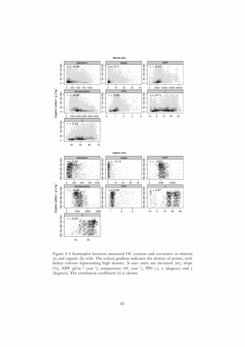
61

Figure 4-3 Scatterplot between measured OC content and covariates in mineral (a) and organic (b) soils. The colour gradient indicates the density of points, with darker colours representing high density. X-axes units are elevation (m), slope (%), NPP (gCm − 2 year − 1), temperature (∘C year − 1), PP0 (-), x (degrees) and y (degrees). The correlation coefficient (r) is shown.

62

4.4.2. OC model

Calibration of the model.

A Gamma distribution was chosen for the GAM as OC content was

continuous and strictly positive. Identity and log-link function were tested. The

analysis of the residuals’ Quantile-Quantile (Q-Q) plot showed better results

with the log-link function which was therefore chosen for the model fitting

(results not shown). The more-or-less straight line observed on the Q-Q plot of

the calibration residuals suggests an approximate Gamma distribution of the

regression residuals (Figure 4-4). The curved pattern with slope increasing from

left to right suggests that the distribution is skewed to the right. The plot

highlights the potential weakness of the chosen distribution towards large OC

values. The backward stepwise selection of the covariates showed that elevation

and PP0 were influencing the prediction model the least (Table 4-2). Slope,

temperature, NPP, land cover, longitude and latitude were selected as

covariates for the final regression model.

Figure 4-4 QQplot of the calibration residuals. The straight line represents the case where the residuals would strictly follow a Gamma distribution.

63

The interaction between latitude and longitude was included in the model using

a non-parametric function in two features using smooth interaction as scale-

invariant tensor products (Wood, 2006b). The interaction accounts for the fact

that the two variables belong to the same physical feature space. Elevation is

often interpretable as a proxy for climatic variables in regression models

predicting soil properties. The presence of temperature data in our model

probably justifies the removal of elevation by the stepwise selection procedure.

The correlation of −0.52 observed between temperature and PP0 explains the

loss of the latter variable during the selection (Table 4-1). The variation in AIC

scores calculated after the removal of each covariate from the model revealed

that land cover is by far the most influential covariate in the model (Table 4-2).

Table 4-2 Summary table of the GAM models tested by backward step-wise removal of the covariates. The difference in Akaike Information Criterion (AIC) scores and deviance explained were calculated.

xy Corine Elev Slope Temp PP0 NPP ΔAIC Δdev explained

x x x x x x x 0 0

x x x x x x 178 0.7

x

x x x x x 1976 6.6 x x

x x x x 16 0.1

x x x

x x x 49 0.2 x x x x

x x 63 0.2

x x x x x

x 19 0.1 x x x x x x 126 0.4

Several authors have also recognised the important influence of land use and

land cover on a soil’s organic carbon pool (Jones et al., 2005; Meersmans et al.,

2011). The combination of longitude and latitude was the second most

influencing variable, followed by net primary productivity. The ‘fitting

performance’ (R2) was 0.29, which is similar to values found by Meersmans et

64

al. (2011). As well as the model performance, the smooth function presented in

Figure 4-5 illustrates the estimated effects of the annual accumulated

temperature (AAT) on OC content. The y-axis is the centered value (log scale)

of the regression coefficients.

Figure 4-5 Smooth function of temperature as produced by the GAM model. The solid line is the predicted value of OC content as a function of temperature. The upper and lower dashed lines are the 95% confidence interval. The bar at the bottom of the graph indicates the presence or absence of a sample.

Overall, OC content decreases as AAT increases, with a rapid decline observed

between 1000 and 2000 °C year-1 and then a slower decline for AAT greater

than 2000 °C year-1. The decrease in decomposition rate with increasing

temperature has been explained by Arrhenius (1889). Below 1000 °C year-1,

however, we observed an opposite trend as OC content increases with

temperature. Areas where these low temperatures were recorded include the

north of Scotland, Finland and Sweden, where the smallest values of NPP were

also observed. The increase in OC content as AAT increases in these cold

65

regions is related to the increase in vegetation cover that contributes to OC

input. The small number of samples taken in these temperature conditions

(shown on the bottom bar) and the large confidence interval observed

encouraged us to regard this last trend with caution.

Model validation.

The validation of the model gave an R2 value of 0.27, which is comparable to

coefficients obtained in similar studies (Meersmans et al., 2011; Kumar et al.,

2012). We believe that the relatively poor model fitting that we obtained was

because of the complexity of the processes of OC accretion and mineralisation

operating at different spatial scales and the great variety of landscapes and soil

types found across Europe (Arrouays et al., 2012). Also, the covariates, having a

resolution of 500 m, may not be able to explain the exact conditions

encountered at the validation profile. For instance, CORINE gives the

dominant land cover, but mixed pixels are common and hence the observed

land cover for the validation profile might not correspond to the CORINE

class. More generally, OC variations occurring at scales smaller than the grid

size of the map cannot be captured by the model and will not be depicted in

the map. Predicted values plotted against observed OC contents had poor

results for Scandinavia (R2 = 0.09), but the remaining countries had better

results (R2=0.28). In those northern latitudes, the model performance was poor

for the prediction of both mineral and organic soils (Figure 4-6). Olsson et al.

(2009) and Heikkinen et al. (2013) showed that, in Sweden and Finland, OC

contents in mineral soils tend to decrease as latitude increases, contrary to what

is observed in other parts of Europe. Although the results of temperature

smoothing indicate an increase in OC content with temperature in those

regions (Figure 4-5), the north to south increase in OC content in mineral soils

of Scandinavia is not well predicted (Figure 4-6b). The presence of organic soils

at those latitudes is probably partly responsible for that, by putting a bias on the

model towards large OC contents. As for the difficulty in predicting OC

content larger than 200 g kg-1, we observe that most organic soils in Europe are

66

Figu

re 4

-6 P

redi

cted

val

ues

plot

ted

agai

nst

obse

rved

OC

con

tent

s in

the

val

idat

ion

set.

Oth

er c

ount

ries

(a)

and

Scan

dina

via

(b).

67

in fact under-predicted (Figure 4-6 a, b). This can be explained by the unimodal

distribution used by the model, whose mean value is tilted towards the vast

majority of residuals coming from mineral soils, therefore leaving residuals

from the organic part of the population in the tail of the distribution. Rawlins et

al. (2009) encountered similar problems in their study in Northern Ireland and

concluded that mineral and peat soils should be modelled separately. This could

be achieved using for instance the methods developed in Poggio et al. (2013).

Overall, the model had an RMSE of 79 g kg-1 (NRMSE=85%). The model had

an RMSE of 42 g kg-1 and an R2 of 0.21 for the prediction of mineral soils, as

well as an RMSE of 287 g kg-1 and an R2 of 0.06 for organic soils. These results

indicate that the use of a unimodal distribution results in a better prediction of

the mineral soils for which the OC values are in the centre of this distribution.

When considering the land cover classes separately, predictions for croplands

on mineral soils are the most accurate (Table 4-3 ). Croplands represent the

second main land cover type in Europe (after woodlands) by occupying nearly a

quarter of the area and they are distributed evenly across the EU (Eurostat,

2011a). Within the organic soils, the model performs better in woodland, which

is the most common land cover type in Europe, with a 39% share of the total

surface area. Most of the organic soil samples in the calibration set were taken

in woodlands, which may explain the better performance of the model for that

land cover type. Conversely, in mineral soils, the model performed the worst at

predicting OC content in woodlands. A reason for this might be the great

heterogeneity observed in forest soils, with measured OC contents ranging

from 1 to 586 g kg-1. Even slight differences in sampling depth and removal of

the ectorganic horizons can induce large variation in OC content because of the

strong vertical gradient in OC contents of forest soils.

68

Table 4-3 Model accuracy (RMSE, root mean square error, g kg-1) and normalised root mean squared error (NRMSE, %) calculated for mineral and organic soils (OC content > 200 g kg-1) and for each LUCAS land-cover class.

Soils Land cover RMSE

/ g kg-1

NRMSE

/ % n

Mineral Bareland 31 161 54

Mineral Cropland 12 96 965

Mineral Grassland 37 126 653

Mineral Shrub 44 119 68

Mineral Wetlands 245 - 1

Mineral Woodland 74 192 443

Organic Cropland 412 - 1

Organic Grassland 290 320 20

Organic Shrub 289 319 7

Organic Wetlands 183 295 4

Organic Woodland 290 282 108

The normalised root mean square error is calculated as the ratio of the root mean square error and the range of observed values.

4.4.3. OC predictions and standard error maps

The largest OC contents were observed in Ireland, the United Kingdom,

Sweden, Finland, Estonia and Latvia, mostly in wetlands (peat lands),

woodlands and in mountainous areas (Figure 4-7). These findings are in line

with current knowledge on spatial distribution of topsoil OC content in Europe

(Jones et al., 2005).

69

Figure 4-7 Map of predicted topsoil organic carbon content (g kg-1).

The smallest OC concentrations were predicted to be mostly in the

Mediterranean countries and also parts of France, Germany, Poland, the Czech

Republic, Slovakia and Hungary, where the land cover is defined as croplands

or permanent crops. Intensive management practices, as implemented on much

agricultural land in Europe, increase the mineralisation of soil organic matter

and therefore reduce OC contents (Lal, 2002). The visual comparison of the

spatial distribution of organic soils proposed by our model and by Montanarella

et al. (2006) indicates good agreement in Ireland, the United Kingdom,

70

Scandinavia and Baltic countries. However, our model seems to predict fewer

organic soils in the Netherlands and in Poland. The reason for the observed

discrepancies might be the differences in the methods used to produce both

maps. The distribution of organic soils in Europe (Montanarella et al., 2006)

was inferred by using a polygon-based approach, following the identification of

different key soil types within the European Soil Map and data-base (King et al.,

1994; Heineke et al., 1998). Large standard errors are observed in northern

latitudes but also in inland wetlands or moors and heathlands (Figure 4-8). Few

samples were taken in the highlands of Scotland, in Wales, in south-western

Ireland or in northern Sweden and Finland, where OC variation tends,

moreover, to be very large (Figure 1-1). In all these areas, OC predictions have

large standard errors. Mountain ranges such as the Alps (Italy, France and

Austria), the Carpathians (the Czech Republic, Slovakia and Poland), the

Apennines (Italy), the Central Massif and the Vosges (France) and the Pindus

(Greece) had large standard errors in their areas below 1000m altitude (areas

above 1000m altitude were masked out in Figure 4-8). The model, whose

weakness at larger OC contents we understand, failed to predict the generally

large OC content measured in these mountain ranges. Areas where a large

standard error is estimated should be considered with caution. In contrast,

areas where a small standard error is calculated (mostly corresponding to the

croplands of Europe) give predictions of OC content that more accurately

approximate the real values. These areas are therefore the most reliable

predictions in Figure 4-7. The standard error map gave a z-score distribution

with =0.043 and 2 =2.01. These values are, however, biased because of the

skewness of the distribution of residuals and when the right tail values are

excluded =0.013 and 2 =0.91.

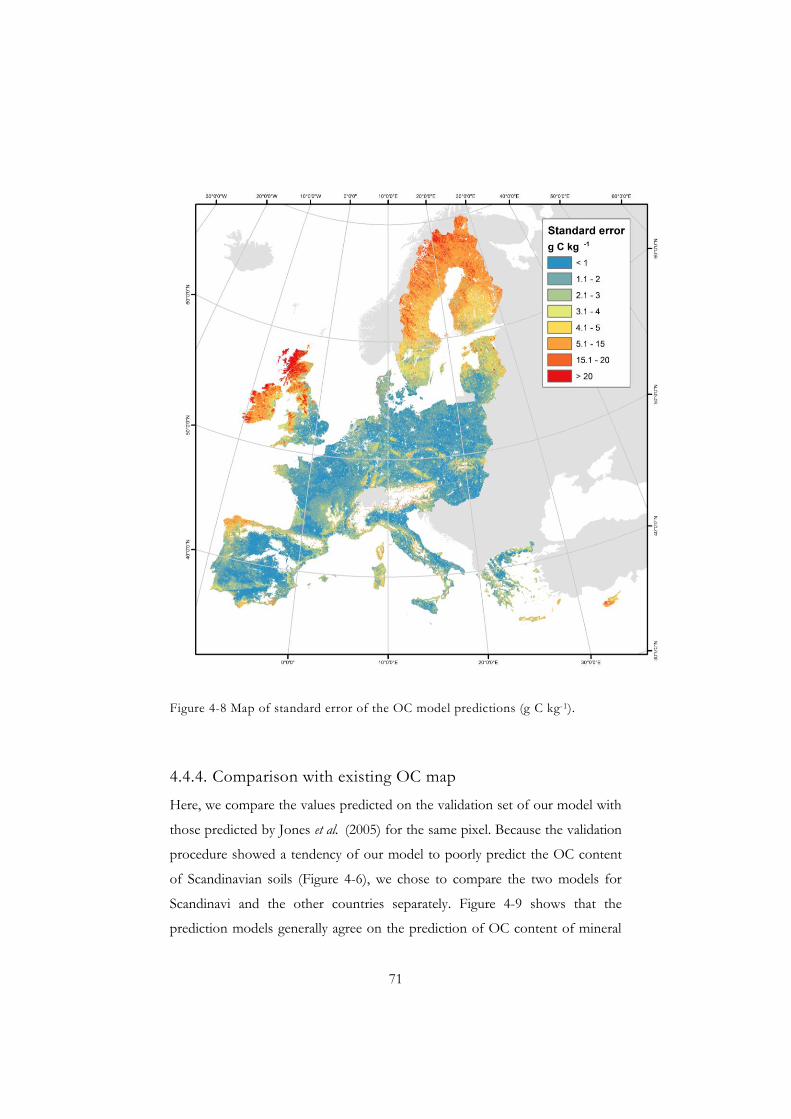
71

Figure 4-8 Map of standard error of the OC model predictions (g C kg-1).

4.4.4. Comparison with existing OC map

Here, we compare the values predicted on the validation set of our model with

those predicted by Jones et al. (2005) for the same pixel. Because the validation

procedure showed a tendency of our model to poorly predict the OC content

of Scandinavian soils (Figure 4-6), we chose to compare the two models for

Scandinavi and the other countries separately. Figure 4-9 shows that the

prediction models generally agree on the prediction of OC content of mineral

72

soils in ‘other countries’. Although the two models were substantially built in

different ways (pedo-transfer rule or regression model), the logic behind their

prediction of OC content is quite similar. Jones et al. (2005) and we recognised

the large influence of land cover and temperature on OC dynamics in soils and

fed the respective models with such information, which led to similar

outcomes. In addition, whilst our input data were actual measured OC values,

OCTOP predicts OC content from measurements from representative soil

profiles synthesised by expert soil scientists from across Europe (King et al.,

1994; Van Ranst et al., 1995). Areas of disagreement are mostly where our

model predicts the OC content for mineral soils whilst the OCTOP model

predicts OC content greater than 200 g kg-1, in Scandinavia, there is not any

clear pattern of agreement or disagreement. The two models can also be

compared on mean OC estimates by land-cover class (Figure 4-10). As the

validation set used for the GAM did not encompass enough points in every

land-cover class to allow for such comparison, we extracted predictions from

the map. Globally, we can see that the average predictions compare well, except

for the inland wetlands class for which the GAM estimates a larger OC

content. The observed match is probably through the use of a common layer in

the prediction models, namely land cover. Also, the error bars are always

smaller in the case of the GAM. Because in OCTOP soil variation is expressed

by discrete soil classes, a mismatch between the large soil units and land cover

classes at larger scales can occur. This creates a more heterogeneous range of

predicted values per land cover class, resulting in wider standard deviations.

The latter supports our initial assumption that OCTOP could be improved by

using more detailed soil spatial information layers or by modelling soil

properties at a finer resolution using DSM techniques.

73

Figu

re 4

-9 S

catte

rplo

t of

OC

con

tent

pre

dict

ions

pro

pose

d by

Jon

es e

t al

. (20

05)

and

by o

ur m

odel

in S

cand

inav

ia (

b) a

nd

othe

r co

untr

ies

(a).

74

Figu

re 4

-10

Com

paris

on o

f m

ean

OC

con

tent

pre

dict

ions

(g

kg-1

) pe

r la

nd-c

over

cla

ss, f

or O

CT

OP

and

for

the

GA

M m

odel

(t

his

stud

y). D

ots

are

mea

n O

C v

alue

s an

d th

e er

ror

bars

rep

rese

nt tw

o st

anda

rd d

evia

tions

(2 )

.

75

4.5. CONCLUSION Our study has proposed the first topsoil OC content map of Europe which is

based on direct harmonised measurements stored in a soil database, produced

using DSM techniques. The model shows a fairly good accuracy for most of the

EU (R2 =0.28), except for Scandinavia (R2 =0.09) where organic topsoils

predominate. This was also indicated by the validation procedure, which

revealed that the unimodal distribution imposed by the fitted model was not

suited to accurately predicting the bimodal distribution of OC content of all

soils in Europe. Hence modelling mineral and organic soils separately might

give better results. However, if the final output is to be spatial, the lack of an

accurate spatial data layer predicting the localisation of organic soils in Europe

will remain a limitation for producing a continuous map using both models.

The comparison of our map with OCTOP underlined the influence of land

cover on OC content in soils and it showed that the use of (discrete) soil classes

instead of continuous fields to express soil OC variation is a major source of

uncertainty. The map produced gives the most up-to-date general picture of

topsoil OC content at the European Union scale and is not intended to be a

substitute for national-scale or local maps that are based on more detailed

spatial information. Moreover, it is important that the uncertainty associated

with the predicted values from this study is understood by the end-users and

should encourage careful use and interpretation of the spatial values.

76

CHAPTER 5. ESTIMATING TOPSOIL ORGANIC

CARBON STOCKS IN EUROPE USING GEO-

REFERENCED HARMONISED TOPSOIL AND

LAND COVER DATA

5.1. ABSTRACT The quantification of soil organic carbon (OC) stocks, and the assessment of

their variability in space and time, have become a common request for soil

scientists, globally. As a consequence to soil being the largest terrestrial carbon

pool, and to the understanding of soil OC major role in the provision of vital

ecosystem services, baseline estimates of soil organic carbon are needed. At the

European Union scale, the only stock estimates available were derived from

harmonised national soil surveys data on OC content estimates (Jones et al.,

2005) combined with bulk density and rock fragment data. In this study, we

proposed baseline estimates of topsoil (0-20 cm) OC stocks in Europe for the

year 2009. Predictions for 23 countries and seven main land cover classes were

generated using 20,000 topsoil OC measurements and 200,000 land cover

observations from the land use/cover area frame statistical survey (LUCAS),

which is the first harmonised topsoil and land cover survey in the European

Union. Several regression models were tested to predict OC content in mineral

soils; whilst average OC measurement values were used for organic soils. A

logistic regression model was built to predict the probability of a soil to be

77

mineral or organic, and to thereafter classify an unknown location as organic or

mineral topsoil. Whilst measurements of gravimetric proportion of rock

fragment were available, bulk density values had to be derived by pedo-transfer

rule. Values of stocks were calculated at 200,000 locations where land cover

observations were available and then extrapolated to countries and land cover

classes. A 95% confidence interval was calculated by bootstrap. The total

estimate, for a 0-20 cm reference depth, is 38.3 Gt with a CI95% ranging

between 34.9 and 42.4 Gt. Our results showed that 35% of Europe’s total OC

stock are stored in Sweden and Finland. In addition, as far as land cover classes

were concerned, woodlands were given as the largest topsoil OC pool in

Europe, with a total of 20.6 Gt (CI95% = ± 7%). The baseline OC stocks

presented here for the year 2009 are the first estimates derived from a

harmonised soil and land cover database at EU scale. The re-conduction of the

LUCAS survey in 2015 and the re-sampling of more than 20,000 topsoil will

allow up-dating the estimates and assessing the effect of a potential land cover

change on topsoil carbon pools.

5.2. INTRODUCTION Because it consists in the largest terrestrial organic carbon reservoir, which can

sequester (sink function) or release (source function) atmospheric CO2, soil is

recognised as having a potential to help mitigate and adapt to climate change

(Batjes, 1996). There is an evident need for data on the status of organic carbon

pools in world soils, whether it be at local scale for agri-environmental

management, at national scale for the reporting of greenhouse gas inventories

to the United Nations Convention on Climate Change or at global scale for

78

providing soil inputs to climatic and environmental models that address crucial

societal challenges. Yet, reliable estimates are lacking.

The quantification of the size of carbon pools requires data on soil OC content,

bulk density and proportion of rock fragments at sampling location. The

reliability of the estimates therefore depends on the accuracy of this input data

and on the sampling density (Martin et al., 2011). The lack of agreement, at any

scale, on harmonised sampling and analytical procedures, in addition to the

rarity of sampling programmes that systematically include measurements of the

necessary parameters, lead to incomplete and inconsistent soil databases that

make accurate OC stocks difficult to estimate. Moreover, the high spatial

variability of OC content requires soil monitoring networks with a high

sampling density, which are expensive and rarely implemented (Saby et al.,

2008).

Traditionally, OC stocks were derived from existing soil maps by attributing

OC values to polygons derived from pedo-transfer rules combining the soil

maps with data layers such as topography, land cover and climate. The OC

values, originating from surveys carried out at different times and following

different methodologies, were used despite the absence of standard method for

combining data and for up- or down scaling it (Krogh et al., 2003). To date,

digital soil mapping techniques (McBratney et al., 2003) have become very

popular to produce estimates of OC stocks and the most recent studies have

been reviewed by Minasny et al. (2013). Digital mapping techniques allow the

production of the uncertainty of estimates and differ from traditional polygon-

based maps in that they are pixel-based (Sanchez et al., 2009). Alternatively, soil

OC dynamics models such as RothC (Coleman & Jenkinson, 1996) or Century

(Parton et al., 1987) have been applied to simulate OC changes for areas with

79

similar climate, soil type and management. Lugato et al. (2014) defined units

with a homogeneous soil and climate throughout Europe and ran the Century

model to estimate the baseline soil OC in these units given the current land

management practice. Furthermore, they simulated the soil OC dynamics under

different land cover scenarios, for time periods going from decades to

centuries.

In Europe, the ENVASSO project which reviewed existing soil monitoring

networks across the EU, defined topsoil OC content and soil OC stocks as

indicators of soil organic matter decline (Arrouays et al., 2008a; Kibblewhite et

al., 2008). The project showed that, although topsoil OC content was one of

the most widely available indicator across the monitoring sites under scrutiny

(Saby et al., 2008), the data was dispersed and not harmonised. Differences in

soil surveying and laboratory analytical methods, together with discrepancies in

dates of the surveys were highlighted as impediment to a joined use of the

national data sets. In addition, bulk density was measured in half of the

countries only. Hiederer (2010) provided the first OC stocks estimates for

Europe, by combining a map of OC content realised during a previous study

(Jones et al., 2005) with bulk density and rock fragments data from the

European Soil Database (ESDB) (King et al., 1994). The data used by Hiederer

(2010) originated from national soil profile surveys, which were heterogeneous

in terms of sampling scheme, analytical procedures and date of collection. The

lack of a harmonised soil database at continental scale was stressed at the same

period as the work of Hiederer (2010), which led to the implementation of the

first European Union (EU)-wide topsoil sampling campaign as a part of the

LUCAS survey. The scheduled repetition of this survey in 2015 (Eurostat,

2014) will mark the establishment of the first harmonised topsoil monitoring

network at European scale.

80

Here we aim at creating a baseline of topsoil OC stocks at the EU scale for the

year 2009, using both the land cover observations and the OC measurements

from the LUCAS survey. As the land cover was recorded in the field during the

LUCAS survey, this information was preferred to data extracted from

CORINE, which unavoidably contains error caused by the spatial interpolation

of point observations to mapping units. As suggested by de Brogniez et al.

(2014), the OC content of mineral and organic soils was modeled separately, as

the bi-modal distribution of the OC data hampered accurate predictions using a

single regression model. Following the definition of histic (organic) soil

horizon, a threshold of 180 g kg-1 OC content will be used as the reference

limit for the presence of organic soils (IUSS Working Group WRB, 2007).

Several regression techniques were then tested to best predict OC content and

a bootstrap approach was implemented to derive confidence intervals and

estimate the uncertainty. Finally, bulk density and rock fragment data were

derived from the LUCAS and ESDB databases and representative surface areas

for each combination of organic/mineral soil and land cover were defined for

the calculation of stocks at national level. We analysed our results and

compared them with those obtained in similar studies. We propose to calculate

OC stocks based on geo-referenced land cover observations and topsoil OC

measurements that originate from a single harmonised database at continental

scale. The method proposed, based on the use of combined land cover and

topsoil sampling networks, allows the calculation of stocks for various types of

spatial units (whether they are continuous or discontinuous in the landscape)

ranging from country level, to land cover class to regional units such as the

European Nomenclature of the Territorial Units for Statistics (NUTS)

(Eurostat, 2011b). The repetition of the LUCAS survey in 2015 will allow

calculation of new stock estimates and therefore offer an over-view of the state

81

and evolution of topsoil carbon pools in Europe, through comparison with the

2009 values.

5.3. MATERIALS AND METHODS In order to calculate topsoil OC stocks we propose different approaches for

mineral and organic soils. A previous study showed that the bi-modal

distribution of the OC data hampered accurate predictions if a single regression

model only was used for all soils (de Brogniez et al., 2014). In addition, the lack

of availability of a harmonised spatial layer that locates organic soils in Europe

was highlighted as a limitation. As opposed to working with a set of continuous

spatial data layers and in order to address the above-mentioned issues, the work

has focussed on point data from the LUCAS and other databases. Figure 5-1

illustrates the methodology followed to predict OC stocks and guides the

reader through the text.

5.3.1. Input data

LUCAS survey

The topsoil OC measurements were used as dependent variable. Land cover

observations for the 200,000 points from the master grid were used as

covariates. Sub-class of land cover was also tested as a covariate where present.

Hence, cropland was sub-classified as cereals, fodder crops, root crops or other

crops; grassland as grassland with sparse tree/shrub cover, grassland without

sparse tree/shrub cover and spontaneously re-vegetated surfaces; woodland as

broadleaved and evergreen woodland, coniferous woodland or mixed

woodland; shrubland as shrubland with sparse tree cover and shrubland

without sparse tree cover.

82

Covariates

Elevation and slope, net primary productivity (NPP), annual accumulated

temperature (AAT), mean annual rainfall were used. We also included in our set

of covariates the World Reference Base (IUSS Working Group WRB, 2007)

reference soil group (e.g. Podzol, Cambisol) and the qualifier (e.g. Umbric,

Mollic, Eutric), extracted from the 1:1,000,000 European soil geographical

database (ESGDB). The reference soil group and the qualifier allocated to

every soil sample correspond to the dominant soil typological unit (STU) in

each soil mapping unit (SMU) corresponding to the polygon where the soil

sample is located. As the ESDB does not cover the islands of Malta and

Cyprus, this study was realised only for the 23 other countries that were

sampled in 2009, during the LUCAS campaign. We refer the reader to Chapter

2 for more details on the covariates.

Rock fragment

In order to calculate the OC stock from a core sample of a known volume, the

rock fragment content by mass (Rm) (that is the gravimetric proportion of

gravels in a sample) must be known. This parameter was measured for the

20,000 topsoil samples of the LUCAS survey.

Bulk density

Bulk density of soils is needed to calculate carbon stocks, but it was not

measured during the LUCAS survey. As clay content (particle size < 2 µm) and

packing density data were available, we calculated bulk density applying the

following equation proposed by Jones et al. (2003) (Figure 5-1, letter A):

Equation 5-1

83

where BDfe is the bulk density of the fine earth (g cm-3), is the packing

density (g cm-3) and C is the clay content (in % mass of the fine earth).

The packing density is a parameter that gives a measure of the apparent

compactness of a soil and was formerly derived in the European soil database,

by applying a pedo-transfer rule (Van Ranst et al., 1995). The packing density

thus obtained for the dominant STU of an SMU was used for the calculations,

together with the clay content which was measured for the LUCAS topsoil

samples and then extrapolated to the 200,000 locations as explained in de

Brogniez et al. (2014).

The bulk density values obtained were judged unsatisfying for the organic soils,

where values ranged between 1.15 and 1.50 g cm-3. The bulk density of peat

depends on the class and type of peat (degree of humification). In Northern

Europe, ombrotrophic peat accumulates as raised moss/bog and blanket bog

because of excess precipitation and slow drainage, whereas mineraotrophic peat

accumulates in hollows, depressions and basins which receive water draining

from surrounding land which does not drain away. Blanket peat forms in the

hills and mountains where decomposition of organic material is slowed by cold

conditions and raised bog form in the lowlands. Analysis of almost 100

measurements of bulk density in the full range of peat types across Ireland

revealed significant differences between the bulk density in the surface horizons

(topsoil) compared to the subsurface (subsoil) horizons. A working average of

0.25 g cm-3 for the former and of 0.12 g cm-3 for the latter were deemed

meaningful for Ireland (R. Jones, personal communication). Another review of

the literature reports an average bulk density of around 0.1 g cm-3 for peat soils

84

85

Figu

re 5

-1 M

etho

dolo

gy f

or th

e ca

lcul

atio

n of

OC

sto

cks,

with

logi

cal f

low

indi

cate

d by

cap

ital l

ette

rs (A

-I).

86

with minima of 0.062 g cm-3 (Tomlinson, 2005). From the conclusions of both

above-mentioned studies, it seemed obvious that our predictions were greatly

overestimating the bulk density in organic-rich soils and that they had to be

modified. It was decided to transform the bulk density of the organic soil

samples (OC content > 180 g kg-1) by applying an equation fitted by Hollis et al.

(2012) (Figure 5-1, letter A):

Equation 5-2

where OC is the OC content (%).

As the bulk density of the total soil sample (fine earth + rock fragment) is

needed to calculate carbon stocks, a last equation was applied (Figure 5-1, letter

B):

Equation 5-3

where BDsample is the bulk density of the total sample (g cm-3), Rm is the rock

fragment content by mass (-), BDr is the bulk density of the rock fragment (g

cm-3) and BDfe is the bulk density of the fine earth (g cm-3).

A value of 2.65 g cm-3 was used as an approximation for BDr as it was not

measured. This value corresponds to the bulk density of quartz and is

commonly used to substitute BDr.

87

Hence,

Equation 5-4

5.3.2. Prediction models

Topsoil organic carbon content

Firstly, we labelled the LUCAS topsoil samples as mineral (measured OC

content < 180 g kg-1) or organic (measured OC content ≥ 180 g kg-1) and

created two subsets based on that criterium (Figure 5-1, letter C). The topsoil

OC content of mineral and organic soils was then predicted following two

different approaches. In the case of minerals soils, the subset was split between a

calibration set (70%) and a validation set (30%). For every land cover class,

three regression models were tested and the best model was selected based on

its coefficient of determination (R2) and root mean squared error (RMSE)

(Figure 5-1, letter D). The three models, namely generalised linear model

(McCullagh & Nelder, 1989), Cubist (Quinlan, 1992) and generalised additive

model (Hastie & Tibshirani, 1986) were tested as they can account for non-

linear relationship between the variable to predict and the covariates, and also

because they can handle non-normal distributions. This latter fact was of major

interest as topsoil OC content does not follow a normal distribution be it in

mineral soils or in organic soils. In addition, Cubist and GAM models have

been recently used by several authors to predict soil OC content (Bui et al.,

2006; Yang et al., 2008; Mayr et al., 2010; Poggio et al., 2013; Roudier et al.,

2014).

88

The covariates were selected by backward stepwise regression, based on the

Akaike Information Criterion (AIC) (Akaike, 1974) of the tested models. As for

organic soils, we decided to use the average measured OC content of the land

cover class where the sample falls as prediction (Figure 5-1, letter E). Hence, as

many estimators of OC content as the combination of two measured soil

classes (mineral vs. organic) and seven land cover classes (cropland, grassland,

bareland, woodland, shrubland, permanent crops, wetlands), that is in total

fourteen models, were produced.

Occurrence of mineral vs. organic soils

A binary logistic regression model was built to predict the probability of a soil

to be organic, as opposed to it being mineral (Figure 5-1, letter F). The

probabilities were estimated by maximum likelihood (ML) as a function of the

covariates and taking an OC content of 180 g kg-1 as a threshold to classify the

observed soils as mineral or organic. It is known that the ML estimation of

logistic models can suffer from unbalanced populations that is from population

where one of the events is rare (King & Zeng, 2001). Because our initial data

set encompassed 18,491 mineral soils and only 1,195 organic soils, we decided

to fit the model on a sample composed of an even amount of mineral and

organic soils. Whilst all the organic samples were kept in the “pool of data”,

1,195 mineral samples were randomly selected. The calibration of the logistic

regression was performed on 70% of those 2390 samples and 30% were kept

aside for the validation procedure. The covariates were selected by backward

stepwise procedure based on the AIC of the different models generated. The

probabilities generated were used to classify a soil as organic or mineral

(hereafter referred to as “soil classes”), choosing a probability of 0.5 as a

threshold for the prediction of one or the other class. Predictions on the whole

data set were made by re-fitting the model, using only the covariates selected by

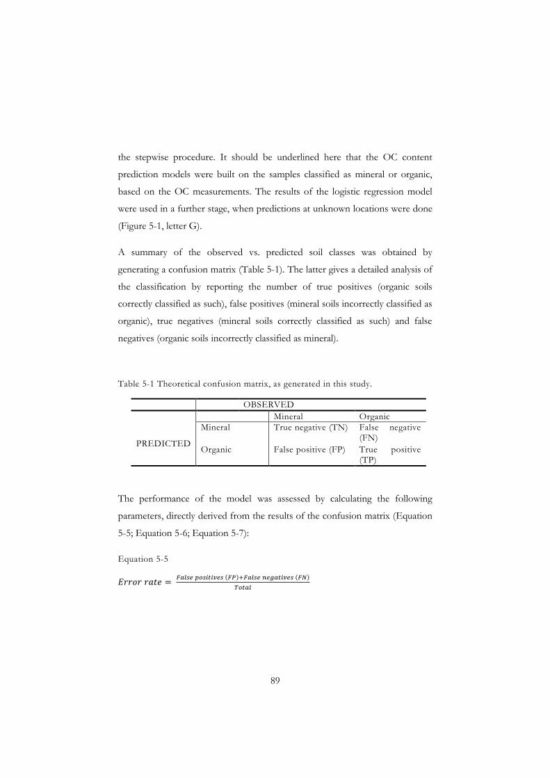
89

the stepwise procedure. It should be underlined here that the OC content

prediction models were built on the samples classified as mineral or organic,

based on the OC measurements. The results of the logistic regression model

were used in a further stage, when predictions at unknown locations were done

(Figure 5-1, letter G).

A summary of the observed vs. predicted soil classes was obtained by

generating a confusion matrix (Table 5-1). The latter gives a detailed analysis of

the classification by reporting the number of true positives (organic soils

correctly classified as such), false positives (mineral soils incorrectly classified as

organic), true negatives (mineral soils correctly classified as such) and false

negatives (organic soils incorrectly classified as mineral).

Table 5-1 Theoretical confusion matrix, as generated in this study.

OBSERVED Mineral Organic

PREDICTED

Mineral True negative (TN) False negative (FN)

Organic False positive (FP) True positive (TP)

The performance of the model was assessed by calculating the following

parameters, directly derived from the results of the confusion matrix (Equation

5-5; Equation 5-6; Equation 5-7):

Equation 5-5

90

Equation 5-6

Equation 5-7

The performance of the model was assessed on the full data set, on the entire

validation set, and for every land cover class within the validation set.

5.3.3. Soil organic carbon stocks

Samples labeling

To calculate the stocks, we assumed that the LUCAS survey gave a

representative picture of the land cover at country scale on the one hand and at

EU scale on the other hand. By applying the logistic regression model on the

200,000 locations of the survey, we obtained predictions of soil classes (Figure

5-1, letter G). We then labeled the samples with a combination of their

predicted soil class (mineral or organic) and the observed land cover class at

that location. Hence, fourteen different labels were created, namely

organic*cropland, organic*grassland, organic*bareland, organic*woodland,

organic*shrubland, organic*permanent crops, mineral*wetlands,

mineral*cropland, mineral*grassland, mineral*bareland, mineral*woodland,

mineral*shrubland, mineral*permanent crops, mineral*wetlands.

91

OC stocks calculation

After having predicted OC content on the predicted mineral or organic soils, by

applying the selected models (Figure 5-1, letter H), we could finally calculate

the total OC stock in the upper 0-20 cm layer of European soils.

To calculate the OC stock, we firstly had to transform the points (of a support

size equals to approximately 12 m2 as the composite sample was taken on 2m

radius around a central point) on which we had worked so far to meaningful

spatial units. To do so, we derived from the points’ statistics the percentage of

the total surface area of every country occupied by each of the fourteen

combinations of soil class*land cover (Figure 5-1, letter I). For instance, if

country A counted 45,000 observations of which 5000 were labeled as

mineral*woodland, we considered that one ninth (5000/45,000) of the national

territory was occupied by mineral*woodland soils. These proportions were used

to calculate the surface area, in km2, occupied by the fourteen classes in every

country. Taking the example of country A, if its total surface area was of 63000

km2, mineral*woodland soils were considered to cover 1/9 of it, that is 7000

km2.

Averages of both predicted OC content and bulk density were calculated for

each of the soil class*land cover combinations at national scale. National OC

stocks were eventually calculated as follows (Equation 5-8):

Equation 5-8

92

where i is the soil class*land cover combination, SOC is the OC content (%),

BDsample is the bulk density of the sample (fine earth and rock fragment) (g cm-

3), S is the surface area (km2), d is the sample depth (20 cm) equal to 0.2 m, Rm

is the rock fragment content by mass (-).

It should be noted that for these calculations, we considered every country to

be fully covered by the soil class*land cover combinations, and we ignored the

presence of urban areas, water bodies, and areas above 1,000 m altitude. These

assumptions introduce an error in the estimation of the total stocks, expressed

in unit of mass (Equation 5-8). However, estimates of stocks expressed as a

mass per unit of surface area, are not affected by these assumptions as the

surface area is not a factor in the equation.

Stocks per land cover class (expressed in unit of mass), at EU scale, were

calculated by summing up national estimates.

Confidence interval

Given the approach followed to derive the soil class (mineral vs/ organic) and

to calculate OC estimates for each combination of soil class*land cover, and in

order to derive confidence intervals for the mean of estimated OC content for

each stratum, a two-stages percentile bootstrap approach was implemented.

The first stage involves the repeated fitting of n logistic models using random

sampling with replacement of the original population of observations for each

stratum. The n models are then used to create a series of classification vectors

where the original population observations are classified as, either organic or

mineral soils. For each of these vectors the subpopulation of mineral soils is

then used in the second stage using it as a sample from which the random

sampling with replacement is applied again, this time to fit the regression model

93

(Cubist, GAM, GLM) predicting the OC content for each observation. The

procedure is then repeated m times to gather a final sample of dimension n·m.

Upon this sample the confidence intervals were calculated using the empirical

distribution percentiles.

For organic soils, the procedure is similar but diverges at stage two, as instead

of fitting a regression model, distribution statistics are calculated directly from

the bootstrapped sampling from the re-classified population.

Mapping OC stocks

OC stocks figures (and their confidence interval) obtained at national scale are

reported on a map to illustrate the trends across the European Member States.

A map of OC stocks per land cover class could however not be generated as

the point-based approach followed for the estimation of the surface areas

covered by every land cover class, did not allow the delineation of areas of

same land cover. The decision to use land cover data coming from field

observations (LUCAS) was motivated by their increased reliability compared to

spatially interpolated data (e.g. CORINE).

94

5.4. RESULTS AND DISCUSSION

5.4.1. Models calibration and validation

GAM, GLM and Cubist regression models were fitted for the prediction of OC

content in mineral soils under every land cover type and the most performant

models were selected (Table 5-2). Because only 20 topsoil samples were

collected in mineral wetlands (Table 5-3), it was decided to calculate an average

value of the measured OC content as its predictor. Results showed that the

Cubist rule-based regression method outperformed the other models in

croplands, that a GLM was selected for predictions in bareland and shrubland

whilst a GAM performed the best for predictions in grassland and woodland.

The comparison of the performance of these selected models (Table 5-2) with

the performance (on the validation set) of the GAM model used in the

previous chapter (Table 4-3) shows a clear advantage in creating a different

model for each land cover class for the prediction of OC content in mineral

soils. RMSEs obtained by fitting a different model for each land cover class are

always lower than with the GAM model. Moreover, the overall R2 for mineral

soils with the GAM is 0.21 (see section 4.4.2) whilst it is 0.59 with the approach

followed in the present chapter. The differences in performance observed can

easily be explained by two facts. Firstly, the fitting of the GAM model on the

whole sample (mineral and organic soils taken together) generated issues for the

prediction of mineral soils in Scandinavia (Figure 4-6) and thereby decreased

the overall performance of the model for these soils. Secondly, the use of land

cover as a discrete covariate in the GAM model allowed accounting for land

cover influence on OC content, only in the intercept of the regression curve

whilst the fitting of separate models for the different land cover classes allowed

95

different slopes (and different intercepts) for the regression curves, which led

to a better accuracy of the predictions.

The covariates selection procedure retained NPP, temperature and rainfall for

all the above-mentioned models (Table 5-4). Moreover, prediction models for

cropland, woodland, grassland and permanent crops selected all the covariates

as of significant influence,

Table 5-2 Summary table for the goodness-of fit and error of the selected best prediction models for OC content (in mineral soils).

Calibration Validation Land cover Model R2 RMSE

(g C kg-1) R2 RMSE

(g C kg-1) Bareland GLM 0.26 19.8 0.36 22.8 Cropland Cubist 0.27 12.1 0.29 10.4 Permanent crops GAM 0.25 10.1 0.16 9.4 Grassland GAM 0.25 21.7 0.22 22.7 Shrubland GLM 0.16 28.1 0.10 28.5 Woodland GAM 0.17 32.7 0.13 32.3 Overall R2 = 0.59

96

Table 5-3 Number of samples and summary statistics of measured and predicted OC content for each soil class*land cover type combination. The soil class has to be understood as “measured” for the LUCAS topsoil survey and “predicted” for the LUCAS general survey (200,000 points).

Soil class Land cover n (LUCAS topsoil)

n (LUCAS general survey)

SUMMARY STATISTICS Measured OC (g C kg-1) Predicted OC (g C kg-1) Min mean Max St.dev Min mean Max St.dev

Mineral Bareland 350 3208 1 17 172 24.6 13 32 47 8.8 Mineral Cropland 7768 51056 1 17 179 13.2 11 17 29 4.5 Mineral Permanent

crops 1014 9005 1 16 143 11.3 10 23 80 14.6

Mineral Grassland 4249 39923 1 33 178 25.2 20 33 59 10.8 Mineral Shrubland 423 10065 1 37 176 31.2 24 41 60 8.5 Mineral Woodland 4667 40565 1 45 179 35.6 22 46 111 18.4 Mineral Wetlands 20 134 11 60 156 40.1 - Organic Bareland 8 948 213 322 431 77.6 322 Organic Cropland 37 175 181 306 567 103.1 306 Organic Permanent

crops 0 0 - - - - -

Organic Grassland 131 7928 180 335 543 98.2 335 Organic Shrubland 32 5653 182 349 510 108.2 349 Organic Woodland 918 41491 180 378 587 109.4 378 Organic Wetlands 69 3820 210 453 564 80.8 453

97

Table 5-4 Selected covariates for every model. (nr) means not relevant, when no sub-classification of land cover class was available for a particular class.

Covariates MIN vs. ORG

Mineral bareland

Mineral cropland

Mineral Permanent crops

Mineral grassland

Mineral shrubland

Mineral woodland

Elevation X X X X X Slope X X X X X NPP X X X X X X X Rainfall X X X X X X Temperature X X X X X X Latitude X X X X X Longitude X X X X X Land cover X - - - - - - Sub-levels of Land cover

nr X nr X X

Soil type X X X Qualifier

98

whereas shrubland showed a different selection. Soil qualifiers were dismissed

for all the models. An overall R2 = 0.59 was obtained for observed mineral

soils, whilst in a previous study, we found an overall R2calibration = 0.29 and

R2validation = 0.27, whilst an R2 = 0.21 was obtained for mineral soils only (de

Brogniez et al., 2014). The methodology followed in this study therefore offers

a clear improvement in terms of OC content prediction (Table 5-2).

The logistic regression model was calibrated on 1672 soil samples (836 mineral

and 836 organic) and the stepwise procedure selected elevation, NPP, rainfall,

temperature, longitude and land cover as predictors (Table 5-4). The validation

procedure gave an error rate of 0.20, a sensitivity of 0.87 and a specificity of

0.80. Predictions on the whole data set after re-fitting the model gave similar

results, with an error rate of 0.19, a sensibility of 0.88 and a specificity of 0.80

(Table 5-5). These figures demonstrate the overall capability of the logistic

regression model to predict the occurrence of both soil classes. The validation

procedure also showed that soil classes are best predicted in croplands and

permanent crops, where the error rate is equal to zero (Table 5-2). Cultivated

topsoils tend to have very low OC content, which resulted in the model to

predict, correctly in most cases, a high probability for soil covered by crops to

be mineral. The largest error rate (0.58) was observed in woodlands, for which

55% of the soil samples (3029) were taken in Sweden and Finland. Within this

land cover class, organic soils were well predicted by the logistic regression

model (sensitivity = 0.96), whereas mineral soils’ occurrence was poorly

predicted (specificity = 0.39). Our analysis of the results for the two

Scandinavian countries revealed that although 75% of the samples in

woodlands were mineral, all of them were classified as organic. This large

amount of misclassified mineral soils can be explained by the fact that 75% of

the organic soil samples of the LUCAS survey were taken in Finland and

99

Table 5-5 Confusion matrices and performance tests parameters. TP= true positives, FN = false negatives, FP = false positives, TN = true negatives.

Data set TP FN FP TN Error rate Sensitivity Specificity n Validation 313 46 3481 14174 0.20 0.87 0.80 18014 Full data set 1040 155 3631 14860 0.19 0.87 0.80 19686 Bareland 0 2 33 302 0.10 0 0.90 337 Cropland 0 7 15 7391 0 0 1.00 7413 Permanent crops 0 0 0 966 0 - 1.00 966 Grassland 16 25 575 3465 0.15 0.39 0.86 4081 Shrubland 9 1 91 318 0.22 0.90 0.78 419 Woodland 271 11 2750 1730 0.58 0.96 0.39 4762 Wetlands 17 0 17 2 0.47 1.00 0.11 36

100

Sweden. The logistic regression model therefore saw the values taken by the

explanatory covariates, such as NPP, temperature and rainfall, in these regions

as an “ideal” environment for organic soils and tended to classify most soils in

such conditions as organic. Nevertheless, it should be kept in mind that this

study aims at proposing a harmonised method for predicting OC stocks at EU

scale and the overall performance of the model should therefore take

precedence over localised weaknesses. Further work could focus on the

creation of a local model for Scandinavia, and thereby on the possibility to

obtain a refined logistic regression model for the other countries, as the “bias”

towards the Northern latitude would no longer be present.

It is noteworthy that NPP, temperature and rainfall were selected as meaningful

covariates for all the models. Climate, usually expressed as temperature and

rainfall, has long been recognised as a major soil forming factor (Jenny, 1941)

and more specifically as having an effect on soil OC dynamics (Post et al.,

1982). NPP is the net production of organic matter by plants in an ecosystem

(IPCC, 2000) and is by definition one of the most important component of the

carbon cycle in soils. The selection of those three variables in all models is

therefore not surprising. On the other hand, the dismissal of the data from the

ESDB as covariates is a surprise, as we expected soil reference groups such as

Podzols or Histosols and qualifiers such as Histic or Humic to be deemed

relevant for our classification. An explanation might be that the (unknown)

location within an SMU of the dominant STU, whose properties were

extracted, does not necessarily match with the location where the LUCAS

sample was taken. Traditional soil mapping used to delineate large areas whose

properties were defined by a reference profile. SMUs were delineated by hand,

based on expert local knowledge of soil properties and soil forming factors

such as topography and the underlying geology. The use of such “units” as

101

covariates for a point-based digital soil mapping analysis at European scale

might therefore not be recommended. In addition, the shallow sampling depth

(20 cm) used during the LUCAS survey, and the fact that only one depth was

sampled might have failed to highlight differences in OC content between

horizons, which are characteristic of some soil types (e.g. Podzols). This

probably led to a heterogeneous “picture” of the samples in terms of OC

content within SMUs that hampered the model to use the ESDB data.

5.4.2. Predictions

OC content

Table 5-3 presents a summary of the statistical distribution of measured and

predicted topsoil OC content. Overall, mean observed and predicted values are

similar for all land cover classes, except for bareland. However, the narrower

range (higher minima and lower maxima) and smaller standard deviation of

predicted OC content as compared to the observations within the different

land cover classes stand out. The results of the logistic regression revealed that

75 % of the actual mineral soils predicted as mineral had OC content lower

than 28 g C ∙ kg-1 (results not shown). We can therefore assume that the points

of the LUCAS survey predicted as mineral by the logistic regression model

were in environmental conditions (combination of covariates value) that

referred to “low” OC content values for the fitted model, which would explain

the low maxima. The overall R2 of predicted OC content on predicted mineral

soils is 0.43.

OC stocks

Results at European scale

We computed the descriptive statistics of OC stocks for Europe’ soils in tonnes

of OC per hectare, taking as spatial unit the combination of land cover*soil

102

class within countries. The results ranged between 25 t C ha-1 (predicted in

Greek mineral cropland) and 230 t C ha-1 (predicted in Irish mineral woodland).

The minimum value we obtain is comparable to the minimum OC stock

Doblas-Miranda et al. (2013) observed in dry Mediterranean areas (23 t C ha-1).

In a study carried out in Ireland, Tomlinson (2005) predicted OC stocks

reaching 3000 t C ha-1 in peat bogs, which greatly contrasts with our last result.

The latter study thoroughly assessed the contribution of peat soil to national

stocks and concluded that peat accounts for 53% of Ireland’s soil OC stocks.

As the full depth of peat bogs, which ranged between 60 cm and 750 cm

depending on the peat type, was considered for the assessment, the large

difference between the figure we obtained and the Irish one can be explained.

However, the mean OC stocks we predicted for Irish organic soils (= 185 t C

ha-1) is very similar to the value we can extract from the Irish study, which is

approximately 150 t C ha-1. Our national estimates of OC stocks in Ireland are

in agreement with the findings of Tomlinson (2005), despite the great

difference in depths accounted for in peat soils. At a 20 cm depth, the mean

OC stock for Europe was 119 t C ha-1 and its median was 105 t C ha-1, whilst

25% (1st quartile) of the areas defined had a stock lower than 64 t C ha-1 and

25% (3d quartile) had a stock higher than 185 t C ha-1.

The total OC stocks in the upper 20 cm of European soils were estimated to be

equal to 38.3 Gt, with a 95% confidence interval (CI95) ranging between 34.9

and 42.4 Gt (Table 5-6). If we rescale (by simple rule of three) those estimates

to the most commonly used 0-30 cm depth for stock calculations, we obtain a

global stock of 57.4 Gt (CI95 = 52.4-63.6 Gt) (Table 5-6). This stock, calculated

for 23 EU countries which occupy 2.7% of the total land area on earth,

correspond to 8 % of the global terrestrial carbon stocks as estimated by Batjes

(1996) for the upper 30 cm of soils. Similarly, other authors compared their

103

results with the estimates of Batjes (1996); Tarnocai et al. (2009) estimated

carbon pools of the northern circumpolar permafrost region to be 191.29 Gt

(27% of total stock on 16% of global land area) whilst Viscarra Rossel et al.

(2014) estimated as stock of 25 Gt for the Australian continent (3.5% of total

stock on 5.2% of global land area).

At European scale, the combined work of Jones et al. (2005) and Hiederer

(2010) is the only other study that estimated OC stocks by country, following a

harmonised methodology. Jones et al. (2005) applied a pedo-transfer rule on a

set of spatial data layers, inferring topsoil OC from the combination of soil

properties, land cover and temperature. The calculations were processed on

harmonised spatial data layers on a 1 km x 1 km grid. Hiederer (2010) used

these OC content estimates combined with bulk density and stone content data

extracted from the European soil database to in turn predict national OC

stocks for Europe. The authors estimated the total OC stock in the upper layer

(0-30 cm) of European soils (23 countries of our study) to be equal to 68.2 Gt,

which exceeds by 7.2% the upper limit of our CI95 (= 63.6 Gt). Table 5-6

presents, country by country, the national OC stocks from Hiederer (2010)

together with our own OC stock estimates and the lower and upper limit of

their CI95, all of them adjusted (by rule of three) to a 0-30 cm depth. For the

stocks from Hiederer (2010) beyond our CI95, the importance of the

under/over estimation as compared to our data was calculated as a percentage

of the lower/upper CI95 respectively. The results concurred only for Austria

and Spain, whilst Poland and Luxembourg showed the worst results with

Hiederer (2010) estimating respectively 65% and 50% bigger OC stocks than

the upper limit of our CI95. Overall, the average difference between predictions

of both studies is 11%, where in most cases we predict lower OC stock values

than Hiederer (2010). The coefficient of determination (R2) for the values

104

Table 5-6 Summary table presenting OC stocks for the 23 countries of the study. The columns present, from left to right: the predicted OC stocks for the sampling depth (20 cm) with the lower and upper limits of the 95% confidence interval and the uncertainties (calculated as half the CI95 divided by the mean stock); the predicted OC stocks adjusted to a standard 0-30 cm depth with the lower and upper limits of the 95% confidence interval; the OC stocks calculated by Hiederer (2010).

Stocks (0-20 cm) Stocks (adjusted to 0-30 cm) Hiederer

Standardised difference between the estimates of Hiederer and ours

Country

Lower limit CI95

(Gt C)

Mean stock (Gt C)

Upper limit CI95

(Gt C)

Uncer-tainty (%)

Stock (t ha-1)

Lower limit CI95

Mean stock

Upper limit CI95

AT 0.69 0.82 1.03 20.4 97 1.04 1.24 1.54 1.20 0.0 BE 0.24 0.26 0.29 9.9 84 0.35 0.39 0.43 0.30 -14.9 CZ 0.48 0.54 0.61 12.3 68 0.71 0.81 0.91 1.10 20.5 DE 2.68 2.96 3.29 10.3 83 4.02 4.44 4.94 5.80 17.4 DK 0.42 0.45 0.48 7.6 103 0.63 0.67 0.73 0.60 -4.0 EE 0.66 0.68 0.71 3.4 150 0.99 1.02 1.06 1.50 41.7 ES 1.90 2.33 2.84 20.1 45 2.85 3.49 4.25 3.50 0.0 FI 5.54 5.74 5.94 3.4 169 8.32 8.60 8.90 12.50 40.4 FR 3.72 4.24 4.88 13.6 66 5.59 6.36 7.32 5.00 -10.5 GR 0.51 0.64 0.84 25.2 48 0.77 0.97 1.25 0.60 -21.7 HU 0.39 0.43 0.49 11.7 47 0.58 0.65 0.73 1.00 36.7 IE 1.07 1.14 1.22 6.5 162 1.60 1.71 1.82 1.60 -0.1 IT 1.37 1.70 2.20 24.5 56 2.05 2.55 3.30 2.00 -2.5

105

LT 0.60 0.64 0.68 5.8 98 0.91 0.96 1.02 1.10 8.2 LU 0.018 0.020 0.022 10.4 76 0.027 0.03 0.033 0.05 50.4 LV 0.83 0.87 0.90 4.3 134 1.25 1.30 1.36 1.80 32.7 NL 0.35 0.38 0.41 8.2 101 0.52 0.56 0.61 0.80 30.1 PL 1.88 2.06 2.26 9.1 66 2.82 3.09 3.39 5.60 65.4 PT 0.44 0.53 0.64 18.8 56 0.66 0.79 0.95 0.50 -23.8 SE 7.59 7.84 8.09 3.2 174 11.39 11.76 12.13 13.80 13.7 SI 0.19 0.22 0.26 14.1 108 0.29 0.33 0.38 0.20 -47.8 SK 0.27 0.31 0.35 13.4 62 0.40 0.46 0.53 0.60 13.6 UK 3.16 3.48 4.00 12.2 142 4.74 5.22 6.00 7.10 18.3 TOTAL 34.9 38.3 42.4 52.5 57.4 63.6 68.25

106

predicted by each study equals 0.94 for the national predictions (Figure 5-2).

The potential source of discrepancies between the two studies are manifold: the

origin and type of soil data, the methods applied to calculate OC content and

bulk density, the resolution of spatial data layers do all contribute to the

differences observed. Hiederer (2010) used a pedo-transfer rule developed by

expert knowledge to predict OC content by harmonising measurements stored

in national soil databases, whilst we developed regression models. The OC

contents had been validated (Jones et al., 2005) against soil profile data

originating from an inventory at 5 km interval across England and Wales (>

5500 points) and a survey of agricultural soils in Italy (6779 points), whereas we

calibrated and validated our model on ca. 20,000 soil samples taken across

Europe.

Figure 5-2 Comparison of the national OC stocks (Gt) at a 0-30 cm depth, as predicted in the present study and by Hiederer (2010). The line with equation y = x shows that our analysis underestimates the larger OC stocks as compared to Hiederer. R2 is the coefficient of determination.

107

Results at country scale

Table 5-6, Figure 5-3 and Figure 5-4 summarise the predictions obtained at

country scale and reveal that the country with the largest predicted OC stock

was Sweden, with about 20% of Europe’s total OC stock stored in its topsoil

(174 t C ha-1 and 7.8 Gt, with CI95 = 7.6-8.1 Gt). Sweden is followed by Finland

with 15% (169 t C ha-1 and 5.7 Gt, with CI95 = 5.5-5.9 Gt) of the EU total OC

stocks. These are situated in the most Northern latitudes of Europe, where

climate is cold. These climatic conditions lead to slow rates of C mineralisation

and therefore boost C sequestration in soils. With a total surface area of almost

450,000 km2, Sweden is the third biggest country in the 23 participating

countries, coming after France (ca. 552, 000 km2) and Spain (ca. 506,000 km2).

We estimated that 92% of the Swedish territory is occupied by organic soils,

whereas national experts (Berglund & Berglund, 2010) stated that about 25% of

the territory is covered by peat. Although not all organic soils are necessarily

classed peat soils, we should assume that our study largely overestimates the

area of organic soils in Sweden and that, as already exposed, this is a result of

the logistic regression model we fitted (see section “Models calibration and

validation”). We consequently should assume that national OC stocks for

Sweden are also largely overestimated in our study. However, no values of

stocks estimated with national OC stocks data for Sweden could be found in

the literature to compare with our results. As the present study aims at

proposing a harmonised method for predicting OC stocks at EU scale, it

appears that it will inevitably result in national totals being different from

estimated OC stocks based on national data sets.

Countries with the smallest OC stocks (Table 5-6; Figure 5-4) were

Luxembourg (20 Mt), Slovenia (221 Mt) and Belgium (259 Mt). These countries

are the smallest of the 23 participating to our study, and they are not known for

108

having large areas of organic soils, which explains their small OC stocks. In

terms of stocks expressed per unit of surface area, Spain (45 t C ha-1), Hungary

(47 t C ha-1), Greece (48 t C ha-1) and Italy (56 t C ha-1) showed the lowest

values for the upper 20 cm of soils (Table 5-6; Figure 5-3). The low ranking of

Mediterranean countries is explained by the high rock fragment content

predicted in the soils of these regions, as well as by their low OC content (de

Brogniez et al., 2014). However, it is important to underline that areas above

1,000m altitude were not sampled during the LUCAS survey. Low OC stocks

in Spain, Greece and Italy therefore result from calculations made regardless of

their vast areas of mountain ranges (Pyrenees, Pindos, Alps and Apennines)

which are known to store a lot of carbon in their soils. The absence of data

from the main European mountain ranges such as the Alps, the Pyrenees, the

Pindos and the Carpathians is therefore to be born in mind as a source of

underestimation of the total OC stocks in this study.

The uncertainties of our estimates at national scale (Table 5-6; Figure 5-4)

calculated as half of the CI95 divided by the mean OC stock, were small for

northern European countries and large for Mediterranean countries. Because

we can see the outcome of the bootstrap as the overlapping of two different

continuous distributions, a difference in their frequencies will affect the

estimation of the confidence interval. If for instance we were to classify every

sample as mineral, we would have a distribution with a range from 1 to 180 g C

kg-1. Elsewise, if the model predicts an even number of organic and mineral

soils, the potential range of the data goes from 1 to 600 g C kg-1. Hence, the

largest uncertainty will be observed if we obtain an even population, made of

similar amounts of organic and mineral soils. So, in the case of northern

European countries were we showed (see section “Models calibration and

validation”) that most soils were misclassified as organic, we obtain a narrow

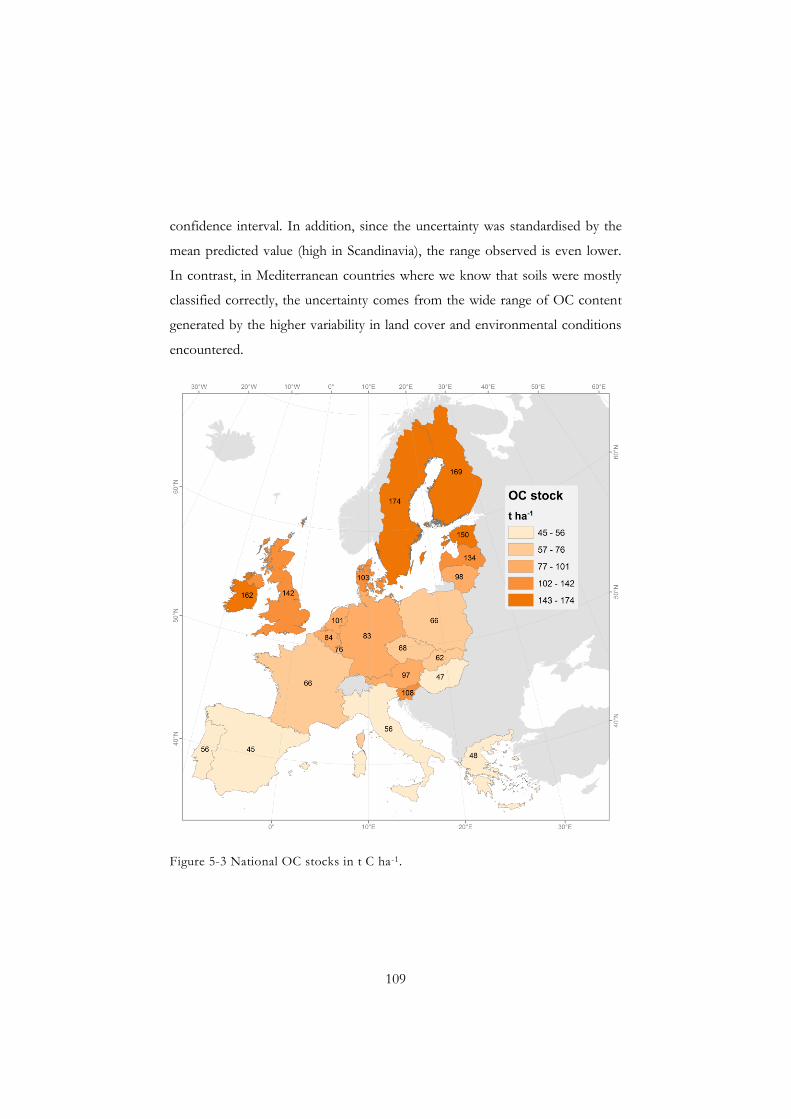
109

confidence interval. In addition, since the uncertainty was standardised by the

mean predicted value (high in Scandinavia), the range observed is even lower.

In contrast, in Mediterranean countries where we know that soils were mostly

classified correctly, the uncertainty comes from the wide range of OC content

generated by the higher variability in land cover and environmental conditions

encountered.

Figure 5-3 National OC stocks in t C ha-1.

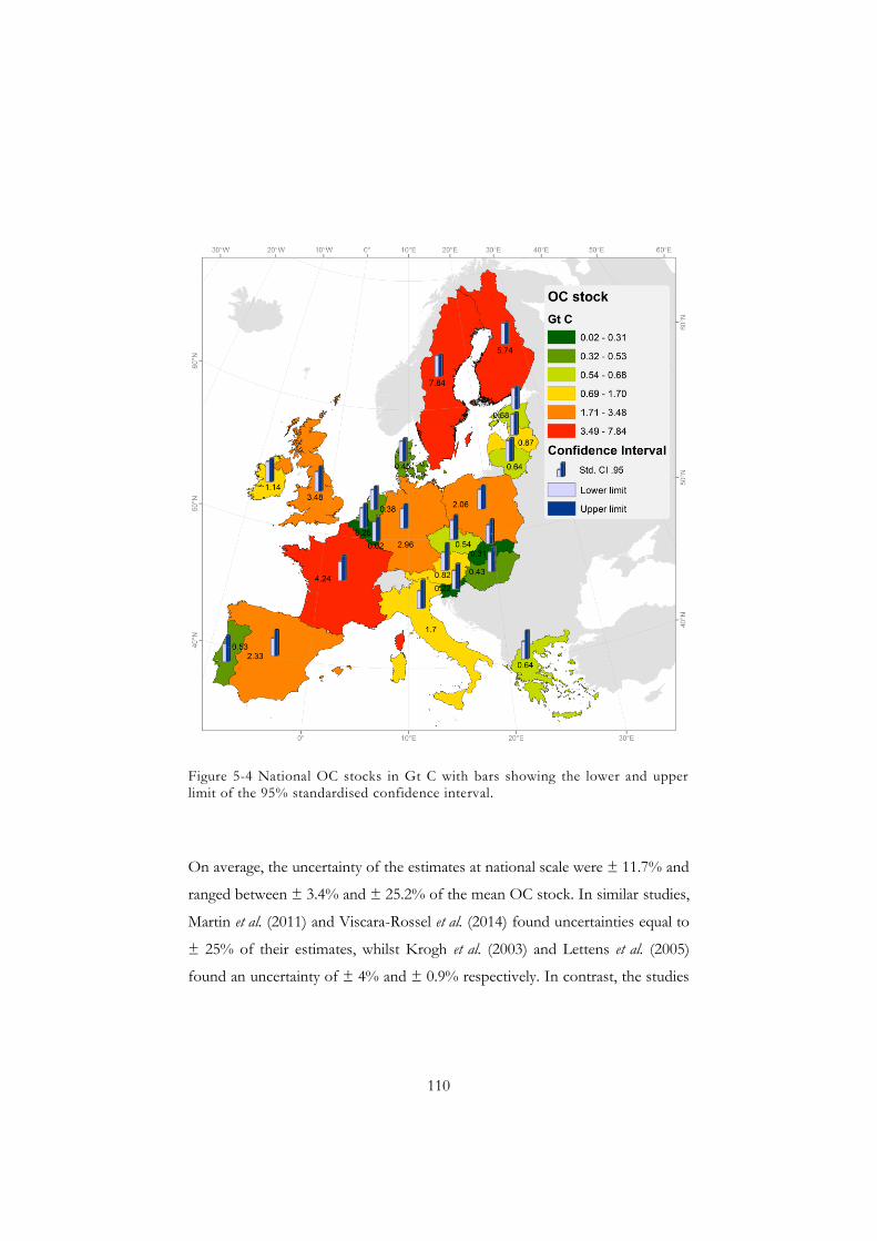
110

Figure 5-4 National OC stocks in Gt C with bars showing the lower and upper limit of the 95% standardised confidence interval.

On average, the uncertainty of the estimates at national scale were ± 11.7% and

ranged between ± 3.4% and ± 25.2% of the mean OC stock. In similar studies,

Martin et al. (2011) and Viscara-Rossel et al. (2014) found uncertainties equal to

± 25% of their estimates, whilst Krogh et al. (2003) and Lettens et al. (2005)

found an uncertainty of ± 4% and ± 0.9% respectively. In contrast, the studies

111

realised by Hiederer (2010) and Tomlinson (2005) did not provide any

confidence interval or estimator of predictions’ reliability. Most studies aiming

at the prediction of soil OC stocks face the challenge of validating results

because soil measurements of OC stocks are rarely (if ever) available.

Consequently, the researchers are left to either assess the uncertainty of their

estimates based on the quality of the input data to their models (Lugato et al.,

2014), or to simply not estimate the uncertainty.

Although most countries in Europe carry out research projects aiming at

predicting national soil OC stocks, notably within the context of the national

inventory report for greenhouse gas emission, only a few of them are published

in scientific literature (Krogh et al., 2003; Tomlinson, 2005; Bradley et al., 2005;

Lettens et al., 2005; Martin et al., 2011). An in-depth comparison of published

national findings with our results was considered outside the scope of this

study.

Results per land cover type

Land use and land cover are widely recognised as amongst the main factors

influencing OC content and stocks in soils. Whilst the former can be defined as

the socioeconomic use made of land (for example, agriculture, commerce,

residential use or recreation), the latter is generally understood as the bio-

physical coverage of land (for example, crops, forest, buildings or roads). Both

factors are connected as a change in land use generally implies a change in land

cover, which in turn affects the plant community as well as soil conditions and

therefore the C cycle in soils (Batjes, 1996; Bolin & Sukumar, 2000). Land

management practices, associated with a certain land use/land cover

combination, have also been demonstrated to greatly influence OC stocks (van

Wesemael et al., 2010). Several agro-ecosystem models such as Century (Parton

112

et al., 1987) and RothC (Coleman & Jenkinson, 1996) were developed to

simulate C dynamics in different land use and in different ecosystems. These

models are able to account for land use change and produce long-term

prediction scenarios of OC stocks. Regression-based techniques, as applied in

this study, have also been widely used in the literature (Smith et al., 2000;

Grimm et al., 2008; Martin et al., 2011; Viscarra Rossel et al., 2014).

Our results gave woodlands as the largest topsoil OC pool in the EU, with a

total of 20.6 Gt (CI95 = ± 7%), which correspond to 54% of the total estimated

stock in Europe (Table 5-7). Woodlands, which occupy 38% of the European

territory (1.56*106 km2), are consequently the primary store of OC stocks in

Europe. Baritz et al. (2010) also highlighted the major importance of forest soils

for the terrestrial carbon pool in Europe, as compared to agricultural soils with

much lower OC contents. These authors analysed the data from the ICP-

Forests soil condition inventory which is, to date, the only project that

attempted to build a harmonised database for forest soils in Europe.

Despite the availability of a manual with recommended procedures for soil

sampling and laboratory analysis, various national modifications of the scheme

proposed by the ICP – Forests inventory were implemented and introduced

systematic errors in the data reported. This again, demonstrated how

challenging it is to establish a harmonised soil-monitoring scheme at large scale.

Nevertheless, Baritz et al. (2010) developed several techniques to render the

heterogeneous data provided by the countries comparable. One of their main

findings was that the investigation of topsoil only was not sufficient to

understand regional patterns of OC (in forests) as some soils, such as Podzols

and Luvisols that accumulate carbon in the subsoil, may appear poorer in

carbon than shallow soils with an organic-rich topsoil. Also, the authors

113

Table 5-7 Summary table of the OC stocks predictions (Gt) per land cover at 20 cm depth. The lower and upper limit of the 95% confidence interval (Gt) , the calculated uncertainty, the occupied surface area (km2) and the OC stock (t ha-1) are also presented.

Lower limit CI95

(Gt)

Mean stock (Gt)

Upper limit CI95

(Gt)

Uncer- tainty (%)

Occupied surface area (km2)

Stock (t ha-1)

Bareland 0,50 0,650 0,80 22,66 77019 84,26 Cropland 3,40 3,82 4,34 12,32 971466 39,35 Grassland 7,58 8,42 9,48 11,24 908453 92,74 Permanent crops 0,49 0,62 0,91 33,70 166398 37,38 Shrubland 2,83 3,16 3,51 10,79 294837 107,26 Wetlands 0,97 1,00 1,03 3,41 73045 137,17 Woodland 19,22 20,59 22,33 7,55 1561702 131,84 Total

38.3

concluded that large C terrestrial pools are located in the European mountain

ranges. These two aspects are important because LUCAS soil samples were

taken down only to a depth of 20 cm and at altitudes lower than 1,000 m.

Whilst the lowest stocks were predicted in permanent croplands with 0.62 Gt ±

34%, woodlands are followed by grasslands and croplands, which account for

22% (8.4 Gt ± 11%) and 10% (3.8 Gt ± 12%) of EU OC stocks respectively

(Table 5-7). In the literature, analysis of OC stocks for agricultural soils (van

Wesemael et al., 2010; Romanyà & Rovira, 2011; Lugato et al., 2014) usually

combines stocks calculated for grasslands (agricultural grasslands only),

croplands and permanent croplands (orchards, vineyards and olive groves). In

the context of the LUCAS survey, grasslands encompass pastures, grassland

under permanent-crops, temporary and artificial grassland, as well as natural

grasslands and fallows; comparison of our results with studies for agricultural

114

soils should be viewed, keeping in mind the more extensive “grassland” pool in

our calculations. If we adjust our results for a 0-30 cm depth, we obtain OC

stock of 59 t C ha-1, 56 t C ha-1 and 139 t C ha-1 for cropland, permanent crops

and grasslands respectively. These values are very similar to those simulated by

Lugato et al. (2014), who ran the agro-ecosystem model Century on almost

164,000 soil-climate-land use combinations to produce OC stocks estimates for

agricultural land in Europe. They obtained a total OC stock of 15.48 Gt for the

same 23 countries as in our study, which is approximately 25% lower than the

total agricultural stock of 19.31 Gt we found. Figure 5-5 (top-graph) shows that

our national estimates are mostly similar to those of Lugato et al. (2014) but that

in a few cases, we indeed predict higher stocks. Those values could probably be

explained by the wider definition of grasslands we adopted, which artificially

increases the agricultural carbon pool. Also, as Lugato et al. (2014) carried out

their study using CORINE land cover which has a specific class for moors and

heathlands, we can hypothesise that very few, if any, organic soils were

accounted for whilst we considered agricultural land covers, regardless of the

soils.

Lugato et al. (2014) estimated the European agricultural land to be of 138 Mha,

whilst we found 189 Mha of agricultural land on mineral soils, and 16 Mha on

organic soils. The latter figures show that a comparison of both studies using

our results for mineral soils only might be a good thing. Indeed, we obtained a

total agricultural soils’ stock of 14.65 Gt on mineral soils, which is much more

similar to what Lugato et al. (2014) found (Table 5-6). Coefficients of

determination (R2) between both studies were calculated to be 0.96 when all

soils are considered and 0.85 for mineral soils only (Figure 5-5). The complete

removal of grasslands in our study leads to a drastic drop of the coefficient of

determination (R2 = 0.67) observed.

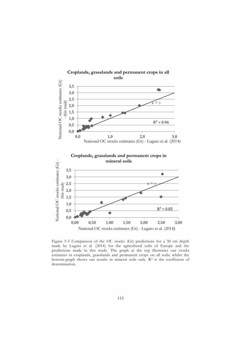
115

Figure 5-5 Comparison of the OC stocks (Gt) predictions for a 30 cm depth made by Lugato et al. (2014) for the agricultural soils of Europe and the predictions made in this study. The graph at the top illustrates our stocks estimates in croplands, grasslands and permanent crops on all soils; whilst the bottom-graph shows our results in mineral soils only. R2 is the coefficient of determination.

0,0 0,5 1,0 1,5 2,0 2,5 3,0 3,5

0,0 1,0 2,0 3,0 Nat

iona

l OC

stoc

ks e

stim

ates

(Gt)

- thi

s stu

dy

National OC stocks estimates (Gt) - Lugato et al. (2014)

Croplands, grasslands and permanent crops in all soils

R² = 0.96

0,0 0,5 1,0 1,5 2,0 2,5 3,0 3,5

0,00 0,50 1,00 1,50 2,00 2,50 3,00 Nat

iona

l OC

stoc

ks e

stim

ates

(Gt)

- th

is st

udy

National OC stocks estimates (Gt) - Lugato et al. (2014)

Croplands, grasslands and permanent crops in mineral soils

R² = 0.85

x = y

x = y

116

Soils under permanent crops and bareland have the highest uncertainties (Table

5-7). The former encompass orchards, berries, olive groves, vineyards and

nurseries according to the LUCAS survey nomenclature. Such crops are usually

managed by leaving strips of bare ground between and around the rows of

trees, which can cause a rather great variety of OC content measured in the

soils, whether the sample is taken under the tree, or in between rows. As far as

bareland is concerned, it has no dominant vegetation on at least 50% of its area

and includes “ecosystems’ as diverse as surfaces covered by mosses and lichens,

bare arable land, temporarily unstocked areas within forests, tidal areas, etc. The

wide range of land use “history” that possibly relates to a bare land explains

how difficult it is to predict its OC level with accuracy. A fallow land with crop

residues or a bare arable land ploughed and ready for seeding will certainly have

different OC content than a tidal surface or a clear-cut on a previously forested

soil.

For more detailed results, we refer the reader to Appendix C, where predictions

per country, land cover type and soil class are given.

5.5. CONCLUSION In this study, we proposed a baseline estimate of soil OC stocks in Europe for

the year 2009, which we generated by following a different approach for

mineral and organic soils. For the first time in the EU, a harmonised topsoil

and land cover database was used to produce OC stocks estimates, which

allowed a meaningful comparison of our results across countries and land cover

classes. Also, as we compared our results with those of other EU studies, we

saw that orders of magnitudes and “contributions” of countries/land cover

classes to the total carbon pool were generally very similar, despite the different

117

approaches followed. Our methodology however showed some limitations in

Northern Europe where the majority of the organic samples of the EU-wide

survey were taken. This most likely led to a great overestimation of the OC

stocks in those latitudes. The lack of availability of a very detailed map locating

organic soils remains a major constraint for the spatial study of soil OC (ESDB

map was tested but gave no significant result). For our predictions, we were

able to define a 95% confidence interval which gives an indication on the

uncertainty of our estimates. Overall, the approach we followed for mineral

soils, using a different model for each land cover class, gave good results in the

validation procedure and we would encourage its application in studies

focussing on mineral soils only.

The calculation of OC stocks crucially depends on bulk density, soil depth and

stone content. These parameters are however rarely measured consistently (if

ever) in soil surveys and they have to be estimated, which introduces significant

uncertainty in the estimation of OC stocks for large areas (e.g, at regional and

national level). Bulk density is ephemeral as it changes significantly with

management and climatic pressures, and accurate estimates should ideally be

revised frequently. Soil depth is key to calculating stocks and, although there

have been debates on whether to work on topsoil or surface soil depth, a fixed

topsoil depth (e.g. 20 cm or 30 cm) is traditionally chosen for comparative

purposes. However, the dynamic nature of surface bulk density has triggered

another debate on whether to use the soil surface as a datum for the

monitoring of OC stocks over space and time. Ellert et al. (2002) demonstrated

that the assessment of OC stock changes on the basis of equivalent soil mass,

by an adjustment of the soil thickness, might be more accurate. Measurements

of stone content for areas of land are even scarcer than for bulk density and

soil depth and their estimates, rarely validated against measurements, are usually

118

considered even more inaccurate than those of bulk density and soil depth. To

these limitations, we should add the lack of precise data on the extent and

depth of organic soils (peat and peaty topped soils), which show different OC

dynamics than mineral soils and should therefore be approached differently for

stock estimates. It seems reasonable to assume that the organic material at

depth is likely to be subject to more change than mineral soil material at the

same depth. Furthermore, the bulk density of peat soil material (0.04 to 0.50 g

cm-3) is much smaller and the range much less than in mineral soils (1.1 to 1.8 g

cm-3) (B. Jones, personal communication). Thus with a much smaller bulk

density, heat transfer is much faster in peat than in mineral material which

influences greatly C mineralisation rate and therefore emissions. Taking all the

above-mentioned considerations into account, there seems to be some merit in

either following the equivalent mass method of soil sampling when possible, or

in restricting the calculation of OC stocks present in a fixed depth of soil,

which we did in the present study (0 - 20 cm). In general, we would consider

that topsoil OC only is worth monitoring because the amount of carbon per

unit depth is much less in the subsoil than in topsoil and because likelihood of

changes in subsoil OC content is much less than in topsoil (except in organic

soils). Moreover, the topsoil layer is after all the soil material most prone to the

effects of climate change. In addition, when accurate in-situ measurements of

bulk density are lacking, it may be expedient to use average bulk densities for

mineral (e.g. 1.3 g cm-3) and organic (e.g. 0.25 g cm-3) topsoils rather than use

complex pedo-transfer functions to estimate bulk density which can have large

uncertainty. Nevertheless, no matter what technique is implemented for the

calculations of stocks, these generally highly uncertain estimates should be

interpreted carefully, keeping the various sources of uncertainties in mind.

119

At a time when mitigation and adaptation strategies to climate change are

sought by policy-makers around the globe, values of soil OC stocks should be

regarded as indicators of the status of soil carbon pools and their potential to

sequester carbon. Given the large sources of uncertainties to stocks estimates,

what is important is not particularly their value per se but the possibility to

produce comparable estimates across countries and over time. The creation of

soil monitoring networks where measures of OC content (at a constant depth)

are recorded to consistently account for the spatial and temporal variability of

those parameters is therefore of major importance for the assessment of

terrestrial carbon pools. In the European context, the re-conduction of the

LUCAS survey scheduled for 2015 will allow updating the baseline we’ve

produced here for the year 2009, and the differences observed will help

assessing the effect of land cover change on soils carbon pools.

121

CONCLUSION

MAIN FINDINGS As the importance of soil OC for ecosystem services and for mitigating climate

change is now clear, the establishment of baseline values to support strategic

environmental management through sound decision making at national and

international level is needed. However, the large spatial variability of soil OC,

together with its slow turn-over, which requires long-term planning of

monitoring systems, make cost-effective and reliable evaluations of soil OC

difficult. Both mapping and accounting help gaining knowledge on the status of

OC in soils; whilst mapping attempts to give a representation of the spatial

distribution of OC in soils, accounting aims at estimating the total amount of

OC in soils, for a particular depth and over a defined area (Minasny et al., 2013).

Knowing the spatial distribution of soil OC can help delineate areas, on the

verge of or undergoing degradation, whereas the quantification of OC stored in

soils relates to the potential of soils to sequester OC and thereby plays a crucial

role in greenhouse gases balance.

In the EU, the absence of a geo-referenced and harmonised data set on soil OC

has hampered a comprehensive assessment of the status of OC in European

soils during the past 40 years. We aimed at producing the most up-to-date

estimates of topsoil OC content and stocks for 25 countries of the European

Union. The following sections explain how the three specific objectives defined

at the beginning of the thesis were met.

122

1. BUILD A HARMONISED SPATIAL DATABASE AT EUROPEAN SCALE

The study of the spatial distribution and the prediction of a soil property

requires the creation of a spatial soil information system. This consists in a geo-

referenced soil database, linked to an attribute database containing measured

values of the particular soil property together with predictive environmental

covariates, relevant to the predictive process and available for the area of

interest (Lagacherie & McBratney, 2007). This study used a combination of

geo-referenced point data (lab analyses of the topsoil samples) collected during

the LUCAS survey and 11 spatially continuous environmental data layers

(covariates) relevant for the prediction of topsoil OC. Regression models were

based on the extracted values of the covariates at the topsoil sampling

locations, while the spatially exhaustive rasters were only used for the creation

of maps. The selection of covariates was restricted by the need to have data

layers that fully covered the study area and were relevant to the year of topsoil

sampling (2009). The creation of such a spatial information system is an asset

for future work as it will allow the addition of new data and it thereby forms

the basis of a dynamic soil information system for Europe. Moreover, as the

system is built as a simple matrix whose rows correspond to a specific location,

the data set can be passed on to scientists from other fields to carry out their

own research.

2. PREDICT AND REPRESENT THE SPATIAL DISTRIBUTION OF TOPSOIL OC CONTENT IN EUROPE, TOGETHER WITH ASSOCIATED UNCERTAINTIES

The first attempt (chapter 3) to represent the spatial distribution of topsoil OC

content (and the uncertainties associated with the predictions) was made by

applying a multiple linear regression between measured soil OC and the

environmental covariates and by kriging the residuals of that regression, with

the OC content predictions resulting from the addition of both models’ results.

123

The second attempt (chapter 4) was made by applying a Generalised Additive

Model (GAM) to the same set of soil and environmental data.

In both chapters, topography (elevation and slope), land cover and temperature

were selected as the most significant covariates. This corroborates the findings

of Minasny et al. (2013) who showed that land use/cover and topographic

features were generally preferred for mapping of topsoil OC. The relevance of

these variables for explaining the variability of soil OC across Europe has been

extensively explained in the different chapters, and references to reviews are

given. However, it is appropriate to highlight the particular relevance of

temperature and land cover in the context of future climatic and demographic

conditions. Davidson & Janssens (2006) showed that the importance of

temperature on soil OC dynamics, an effect that is likely to increase with global

warming; soils that are under current climatic conditions either waterlogged

(peat) or frozen (permafrost) will release substantial amounts of CO2 as their

upper layers dry out or thaw. Moreover, growing world population will

undoubtedly result in increasing conversions of natural or semi-natural land to

arable land or urbanised areas, which in turn will translate into inevitable losses

of soil OC.

The amount of topsoil OC content was shown to increase with latitude in

Europe on both prediction maps, which corroborated the findings of Jones et

al. (2005) and the current knowledge on soil OC status across Europe. Low OC

content was consistently observed in croplands whilst high OC content was

unsurprisingly predicted in woodlands and wetlands. Intensive agricultural

systems that are widespread across Europe, and the potential effect of land

conversion to cropland, are clearly identified here as a cause of low OC content

in soils. On the other hand, the results suggest that the preservation of moors

and heathlands, as well as of forests, would encourage the sequestration of C in

soils.

124

Results showed that the GAM performed better (R2validation = 0.27) than the

regression kriging technique (R2validation = 0.12) and this is most probably due to

the fact that GAM can capture the non-linear relationship between soil OC and

covariates, which are most likely to occur in nature. Moreover, the bi-modality

of the frequency distribution of OC content in the topsoils of Europe, with the

majority of samples being taken in mineral soils, resulted in the underestimation

the OC content of organic soils by both models and in the generation of large

uncertainties in areas where organic soils mostly occur (Scandinavia, UK,

Ireland). Low uncertainties were found in croplands. This latest finding

suggested that the study of mineral and organic soils should be done separately.

3. PROPOSE A METHOD FOR THE QUANTIFICATION OF THE SIZE OF OC POOLS IN EUROPE.

Chapter 5 proposes a methodology for the calculation of OC stocks (Figure

5-1) in Europe, with a confidence interval associated with the predictions. The

method, based on soil and land cover statistics of data collected at geo-

referenced locations, is flexible and applicable to any spatial unit of interest.

The OC stocks were calculated for countries and for land cover classes

throughout Europe, but they could have been obtained just as easily for NUTS

areas or for other delineated areas of particular interest such as national parks,

as long as at least one sample was taken there.

Net Primary Productivity (NPP), temperature and rainfall were selected as

meaningful covariates for all models, whilst data extracted from the European

Soil Database (ESDB) were excluded because the use of relatively large spatial

units such as SMUs (which represent a group of soil associations) might not be

relevant for point-based statistical analyses. The total OC stock in Europe of

38.3 Gt (CI95: 34.9 – 42.4) was predicted for the reference topsoil depth (0-20

cm). One third of that stock was found to be stored in Finland and Sweden,

and woodlands were identified as the land cover storing the largest OC pool of

20.6 Gt (CI95 ± 7%). Overall, the predictions and their confidence intervals

125

obtained for the 23 countries and for main land cover classes were of similar

order of magnitude to those found in studies conducted at national or EU

scale. The use of a logistic regression model to predict the occurrence of

mineral or organic soils gave good results except in woodlands where mineral

soils were most of the time misclassified as organic. This was explained by the

high frequency of organic soils sampled in woodlands which “biased” the

logistic regression model. Building separate models for land cover classes in

mineral soils allowed the prediction performance to increase and therefore this

practice is to be recommended.

LIMITATIONS A series of constraints beset the objectives of this study and these are outlined

below.

Most constraints were related to the use of topsoil data originating from the

LUCAS survey 2009. First of all, no topsoil samples were taken above 1,000 m

altitude, mostly corresponding to extensive areas in the Alps, Apennines,

Pyrenees, Pyndus, Central Massif and Sierra Nevada. Mountain soils are likely

to accumulate substantial amounts of OC because cold temperatures limit

mineralisation of carbon (Sjögersten et al., 2011). It can therefore be expected

that the accounting of soils above 1,000 m altitude in the Alps would have led

to higher total estimates of OC stocks for Europe. Moreover, as climate change

predictions suggest that European mountains will experience increasing

warming in the next century (Nogués-Bravo et al., 2007), the monitoring of the

OC status of their soils should be encouraged.

Secondly, the absence of measurements of bulk density for the LUCAS topsoil

samples was seen as a major impediment to the calculations of OC stocks. This

issue is discussed in the conclusion of chapter 5. Thirdly, the fact that no

resampling campaign of the LUCAS survey was conducted (in 2009) prevented

126

us from performing an independent validation of our predictions. Finally, the

low density of soil sampling based on the 2 km x 2 km LUCAS original grid,

coupled with the relatively coarse resolution of the covariates (500m)

jeopardised our ability to model, understand and therefore explain the spatial

variability of soil OC at short range. Any variation arising from the intrinsic

variability of soil OC (random variability) or from environmental factors whose

effects operate at distances shorter than the spatial resolution and minimum

sampling distance cannot be captured by the spatial model and is therefore

excluded from the assessment (Lagacherie & McBratney, 2007). Whilst

McBratney & Pringle (1999) found that the spatial correlation of soil OC within

a field is between 20 and 300 m, Minasny et al. (2013) showed that the spatial

variation of soil OC, as observed on a variogram, depends on the extent of the

study area. At large scale, it seems likely that the theoretical variogram of soil

OC never reaches a steady-stationarity, but is instead made of a series of

“plateaus”. Each of these plateaus illustrates the consistent influence of an

environmental factor on OC levels at a certain scale.

Besides all the constraints related to the LUCAS survey itself, our investigation

was often limited by the lack of a detailed map delineating organic soils in

Europe. The use of dominant soil types and soil qualifiers extracted from the

European Soil DataBase (ESDB) did not give significant results and no other

data layer at EU scale was found in the literature. As organic soils show

different OC dynamics than mineral soils, which was clearly highlighted in this

research, their study should be approached differently. The selection of

covariates and most importantly, the design of soil sampling strategies targeting

the assessment of OC conditions in either mineral or organic soils is essential.

Last but not least, a broader limitation concerns the use of this thesis’ outputs

and is related to the interpretation of the models accuracy and uncertainty by a

broad range of end-users (policy-makers, land planners, farmers, scientists with

a different expertise, etc.). Because scientific literature (including this work)

127

generally targets an audience of peers, an in-depth discussion of the meaning of

values such as RMSEs or standard errors is often overlooked. The RMSEs tell

us how well the predicted values match the measured values, i.e. the accuracy of

the prediction model. A graph plotting predicted vs. observed values should

always be provided with the results as it illustrates what part of the sample is

well predicted and whether some part of it is under- or over-predicted. As for

the standard error, it relates the variability of the input data with the variability

of the predicted mean output value (OC content in our case), i.e. the

uncertainty of the model. A thorough understanding of these model evaluation

parameters is crucial for a careful use and interpretation of the model outputs.

OUTLOOK This study has produced estimates of topsoil OC stocks and has illustrated the

spatial distribution of topsoil OC content based on laboratory measurements in

25 Member States of the European Union, establishing a baseline for the year

2009. Trends at continental and national scale were highlighted and they are

deemed relevant for policy areas, particularly agriculture and environment.

Moreover, the use of the spatial database resulting from this research as an

input for large scale studies focussing on environmental management and food

security should be promoted. The maps produced may allow the delineation of

vulnerable areas, typically those with low OC content, where “good”

management should be implemented in order to prevent further degradation

going past a point of no return. The management of areas with high OC

content should also be a priority in the context of climate change mitigation

strategies, but also for the benefit of the environment as a whole.

This research has highlighted the importance of sampling soils in the field using

standard protocols and methods of analysis. Land above 1000 m in altitude

must be sampled in the next LUCAS survey if the distribution of the OC

content in soils of the whole of Europe is to be determined. This is essential to

128

obtain more accurate estimates of OC stocks in Europe. Likewise, the

measurement of bulk density and subsoil sampling should enhance our ability

to accurately and comprehensively estimate total OC stocks in Europe,

although this would be impractical in the context of a rapid and large-scale

survey such as the LUCAS.

This research also highlights the importance of establishing a comprehensive

soil monitoring system for Europe. When the repetition of the soil component

of the LUCAS survey is planned, special emphasis should be put on the use of

the same sampling and analytical protocols in order to obtain the first time

series of comparable soil data across Europe. Moreover, to make sure that the

next sample is as equally representative of EU soils as the LUCAS 2009 data,

re-sampling as close as possible to the same locations is essential. Research has

already shown that a sampling interval of 10 years is appropriate for soil OC

(Arrouays et al., 2008b) and this should be kept in mind when the analyses of

the LUCAS 2015 topsoil samples will be made available. If no better resolution

of covariates and if no new data relevant for the study of OC are available, the

reproduction of maps and the re-calculation of OC stocks using spatial

interpolation techniques at EU scale will most probably show similar, if not

identical, results as those produced in this thesis. However, this assumption

should be verified by comparing the distribution of the OC content data from

2009 and 2015. The use of cumulative distribution functions or histograms,

together with basic descriptive statistics will allow this comparison and should

determine the next step of the study. If the distributions of measured OC

content data are identical, and if the same covariates as in 2009 are available,

the creation of new models and maps of OC content will most probably be a

waste of time. In this case, we’d advise a second-round of soil sampling, which

should occur in areas where large uncertainties were predicted in 2009. By

doing so, a refined understanding of the distribution of OC content will be

acquired and new predictions should therefore be informative. If the

distributions of 2009 and 2015 differ, then a similar study to the one presented

129

in this thesis could be performed. Moreover, the difference between measured

values in 2009 and 2015 could be used as a new variable of which the spatial

variability could be studied.

Last but not least, increasing the sampling density (on more than 10% of the

LUCAS original sites) should be considered. Areas where the frequency of

organic soils (in the LUCAS 2009) is high should be given priority for denser

sampling, to better estimate the statistical distribution of OC content in such

soils. Moreover, having sub-samples of closely spaced point-pairs (< 2 km)

across Europe would allow the calculation of OC content variogram at short

scale and the estimation of its nugget. Such variogram would in principle

improve the understanding of the spatial variability of OC in soils by

differentiating the intrinsic soil OC variability from the variation caused by

environmental features (such as topography) at short scale.

130

REFERENCES

Akaike, H. 1974. A new look at the statistical model identification. IEEE Transactions on Automatic Control 19, 716–723.

Arrhenius, S. 1889. Uber die Reaktionsgeschwindigkeit bei der Inversion von Rohrzucker durch Sauren. Zeitschrift für Physikalische Chemie, 226–248.

Arrouays, D., Deslais, W., & Badeau, V. 2001. The carbon content of topsoil and its geographical distribution in France. Soil Use and Management 17, 7–11.

Arrouays, D., Jolivet, C., Boulonne, L., Bodineau, G., Ratié, C., Saby, N. & Grolleau, E. Le Réseau de Mesure de la Qualité des Sols (RMQS) de France. 2003. Etude et Gestion des Sols 10, 241-250.

Arrouays, D., Marchant, B.P., Saby, N.P.A., Meersmans, J., Orton, T.G., Martin, M.P., Bellamy, P.H., Lark, R.M., & Kibblewhite, M. 2012. Generic issues on broad-scale soil monitoring schemes: A review. Pedosphere 22, 456–469.

Arrouays, D., Morvan, X., Saby, N.P.A., Richer de Forges, A., Bellamy, P., Berényi Üveges, P.H., Freudenschuß, J., et al. 2008a. Environmental Assessment of Soil for Monitoring - Volume IIa. Inventory and Monitoring. Office for Official Publications of the European Communities, Luxembourg.

Arrouays, D., Richer de Forges, A., Morvan, X., Saby, N.P.A., Jones, A.R., & Le Bas, C. 2008b. Environmental Assessment of Soil for Monitoring - Volume IIb. Survey of National Networks. Office for Official Publications of the European Communities, Luxembourg.

Asch, K. 2003. The 1:5 Million International Geological Map of Europe and Adjacent Areas: Development and Implementation of a GIS-enabled Concept. E. Schweizerbart, Stuttgart.

131

Banwart, S., Black, H., Cai, Z., Gicheru, P., Joosten, H., Victoria, R., Milne, E., et al. 2014. Benefits of soil carbon: report on the outcomes of an international scientific committee on problems of the environment rapid assessment workshop. Carbon Management 5, 185–192.

Baritz, R., Seufert, G., Montanarella, L., & Van Ranst, E. 2010. Carbon concentrations and stocks in forest soils of Europe. Forest Ecology and Management 260, 262–277.

Baritz, R., Zirlewagen, D., Jones, R., Arrouays, D., Hiederer, R., Schrumpf, M., & Riek, W. 2011. Carbon in European Soils. p. 49–84. In Jandl, R., Rodeghiero, M., Olsson, M. (eds.), Soil Carbon in Sensitive European Ecosystems. John Wiley & Sons, Ltd, Chichester, UK.

Batjes, N. h. 1996. Total carbon and nitrogen in the soils of the world. European Journal of Soil Science 47, 151–163.

Bellamy, P.H., Loveland, P.J., Bradley, R.I., Lark, R.M., & Kirk, G.J.D. 2005. Carbon losses from all soils across England and Wales 1978–2003. Nature 437, 245–248.

Berglund, Ö., & Berglund, K. 2010. Distribution and cultivation intensity of agricultural peat and gyttja soils in Sweden and estimation of greenhouse gas emissions from cultivated peat soils. Geoderma 154, 173–180.

Bisutti, I., Hilke, I. & Raessler, M. 2004. Determination of total organic carbon – an overview of current methods. Trac-Trends in Analytical Chemistry 23, 716–726.

Bolin, B., & Sukumar, R. 2000. Global perspectives. p. 23–51. In Land use, land use change and forestry. Cambridge university press, Cambridge, UK.

Bouma, J., & Van Lanen, H.A.J. 1987. Transfer functions and threshold values: from soil characteristics to soil qualities. p. 106–110. In Beek, K.J., Burrough, P.A., McCormack, D.E. (eds.), Quantified Land Evaluation Procedures. ITC Publications.

Bradley, R.I., Milne, R., Bell, J., Lilly, A., Jordan, C., & Higgins, A. 2005. A soil carbon and land use database for the United Kingdom. Soil Use and Management 21, 363–369.

132

de Brogniez, D., Ballabio, C., Stevens, A., Jones, R.J.A., Montanarella, L., & van Wesemael, B. 2014. A map of the topsoil organic carbon content of Europe generated by a generalized additive model. European Journal of Soil Science, n/a–n/a.

Bui, E.N., Henderson, B.L., & Viergever, K. 2006. Knowledge discovery from models of soil properties developed through data mining. Ecological Modelling 191, 431–446.

Chen, F., Kissel, D.E., West, L.T., Adkins, W., Rickman, D., & Luvall, J.C. 2008. Mapping soil organic carbon concentrations for multiple fields with image similarity analysis. Soil Science Society of America Journal 72, 186 – 193.

Cheshire, M.V., Dumat, C., Fraser, A.R., Hillier, S., & Staunton, S. 2000. The interaction between soil organic matter and soil clay minerals by selective removal and controlled addition of organic matter. European Journal of Soil Science 51, 497–509.

Christensen, B.T. 2001. Physical fractionation of soil and structural and functional complexity in organic matter turnover. European Journal of Soil Science 52, 345–353.

Coleman, K., & Jenkinson, D.S. 1996. RothC-26.3 - A Model for the turnover of carbon in soil. p. 237–246. In Powlson, D., Smith, P., Smith, J. (eds.), Evaluation of Soil Organic Matter Models. NATO ASI Series. Springer Berlin Heidelberg.

Commission of the European Communities. 1995. CORINE land cover - part 1: Methodology. Available at http://www.eea.europa.eu/publications/COR0-landcover (verified 21 November 2014).

Daroussin, J. 2003. Appendix I: Selection of interpolation method for meteorological data for the PESERA project. p. 34. In Irvine, B.J., Kosmas, C. (eds.), PESERA User’s Manual. PESERA, European Commission funded fifth framework project - contract QLK5-CT- 1999-01323.

Davidson, E.A., & Janssens, I.A. 2006. Temperature sensitivity of soil carbon decomposition and feedbacks to climate change. Nature 440, 165–173.

de Gruijter, J.J., Brus, D.J., Bierkens, M. & Knotters, M. 2006. “Introduction.” In Sampling for Natural Resource Monitoring, 1-9. Springer Berlin Heidelberg.

133

Doblas-Miranda, E., Rovira, P., Brotons, L., Martínez-Vilalta, J., Retana, J., Pla, M., & Vayreda, J. 2013. Soil carbon stocks and their variability across the forests, shrublands and grasslands of peninsular Spain. Biogeosciences 10, 8353–8361.

Doran, J.W., & Parkin, T.B. 1994. Defining and Assessing Soil Quality. p. 1-21. In Defining Soil Quality for a Sustainable Environment. Soil Science Society of America Sepcial Publication n35.

Ellert, B.H., Janzen, H.H. & Entz T. 2002. Assessment of a method to measure temporal change in soil carbon storage. Soil Science Society of America Journal 66, 1687–1695.

European Commission. 2002. Communication from the Commission to the Council, the European Parliament, the Economic and Social Committee and the Committee of the Regions: Towards a Thematic Strategy for Soil Protection. European Commission, Brussels.

European Commission. 2006a. Proposal for a Directive of the European Parliament and of the Council establishing a framework for the protection of soil and amending Directive 2004/35/EC. European Commission, Brussels.

European Commission. 2006b. Communication from the Commission to the European Parliament, the Council, the European Economic and Social Committee and the Committee of the Regions Thematic Strategy for Soil Protection. European Commission, Brussels.

European Environment Agency. 2012. Corine Land Cover 2006. Available at http://sia.eionet.europa.eu/CLC2006 (verified 21 November 2014).

Eurostat. 2009a. LUCAS 2009 (Land Use/Cover Area Frame Survey) -Technical reference document C-3: Land use and land cover, nomenclature. Luxembourg.

Eurostat. 2009b. LUCAS 2009 (Land Use/Cover Area Frame Survey). Technical reference document C - 1. Instruction for surveyors.

Eurostat. 2011a. Land cover and land use statistics at regional level. Available at http://epp.eurostat.ec.europa.eu/statistics_explained/index.php/Land_cover_and_land_use_statistics_at_regional_level#Further_Eurostat_information (verified 14 November 2013).

Eurostat. 2011b. Regions in the European Union. Nomenclature of territorial units for statistics. Available at

134

http://epp.eurostat.ec.europa.eu/cache/ITY_OFFPUB/KS-RA-11-011/EN/KS-RA-11-011-EN.PDF (verified 24 November 2014).

Eurostat. 2013. Land cover/use statistics. Available at http://epp.eurostat.ec.europa.eu/portal/page/portal/lucas/introduction (verified 16 October 2014).

Eurostat. 2014. Invitation to tender for the supply of statistical services. Land use/cover area frame statistical survey (LUCAS) 2015 - Agri-environmental survey: field work, technical assistance and quality control.

FAO-UNESCO. 1974. FAO-Unesco Soil Map of the World - 1:5 000 000. UNESCO, Paris.

Farr, T.G., Rosen, P.A., Caro, E., Crippen, R., Duren, R., Hensley, S., Kobrick, M., et al. 2007. The Shuttle Radar Topography Mission. Reviews of Geophysics 45.

Garten, C.T.J., & Hanson, P.J. 2006. Measured forest soil C stocks and estimated turnover times along an elevation gradient. Geoderma 136, 342 – 352.

Grimm, R., Behrens, T., Märker, M., & Elsenbeer, H. 2008. Soil organic carbon concentrations and stocks on Barro Colorado Island — Digital soil mapping using Random Forests analysis. Geoderma 146, 102–113.

Grunwald, S. 2009. Multi-criteria characterization of recent digital soil mapping and modeling approaches. Geoderma 152, 195–207.

Guo, L.B., & Gifford, R.M. 2002. Soil carbon stocks and land use change: a meta analysis. Global Change Biology 8, 345–360.

Hallett, P.D., Loades, K.W., & Krümmelbein, J. 2012. Chapter 9. Soil Physical Degradation: Threats and Opportunities to Food Security. p. 198–226. In Hester, R.E., Harrison, R.M. (eds.), Soils and Food Security. Royal Society of Chemistry, Cambridge.

Hastie, T., & Tibshirani, R. 1986. Generalized Additive Models. Statistical Science 1, 297–318.

Hastie, T., Tibshirani, R., & Friedman, J. 2009. The Elements of Statistical Learning: Data Mining, Inference, and Prediction. Second. Springer, New-York, USA.

135

Heikkinen, J., Ketoja, E., Nuutinen, V., & Regina, K. 2013. Declining trend of carbon in Finnish cropland soils in 1974–2009. Global Change Biology 19, 1456–1469.

Heineke, H.J., Eckelmann, W., Thomasson, A.J., Jones, R.J.A., Montanarella, L., & Buckley, B. 1998. Land Information Systems: Developments for Planning the Sustainable Use of Land Resources. Office for Official Publications of the European Communities, Luxembourg.

Hempel, J., McBratney, A.B., Arrouays, D., McKenzie, N., Hartemink, A.E., Grundy, M., Greve, M., et al. 2014. GlobalSoilMap and Global Carbon Predictions. p. 363–372. In Hartemink, A.E., McSweeney, K. (eds.), Soil Carbon. Progress in Soil Science. Springer International Publishing.

Hiederer, R. 2010. Organic carbon in topsoils (0 - 30 cm) per country in peta grams [Pg]. Available at http://eusoils.jrc.ec.europa.eu/esdb_archive/octop/Resources/OC_Per_Country.pdf (verified 21 November 2014).

Hijmans, R.J., Cameron, S.E., Parra, J.L., Jones, P.G., & Jarvis, A. 2005. Very high resolution interpolated climate surfaces for global land areas. International Journal of Climatology 25, 1965–1978.

Hollis, J.M., Lilly, A., Higgins, A., Jones, R.J.A., Keay, C.A., & Bellamy, P. 2014. Predicting the water retention characteristics of UK mineral soils. European Journal of Soil Science, n/a–n/a.

Howard, P.J.A., Loveland, P.J., Bradley, R.I., Dry, F.T., Howard, D.M., & Howard, D.C. 1995. The carbon content of soil and its geographical distribution in Great Britain. Soil Use and Management 11, 9–15.

Huber, S., Prokop, G., Arrouays, D., Banko, G., Bispo, A., Jones, R.J.A., Kibblewhite, M.G., et al. 2008. Environmental Assessment of Soil for Monitoring - Volume I. Indicators & Criteria. Office for Official Publications of the European Communities, Luxembourg.

IPCC. 2000. Global perspective. p. 375. In Land use, land use change and forestry. Cambridge university press, UK.

IUSS Working Group WRB. 2007. World Reference Base for Soil Resources 2006, first update 2007. FAO, Rome.

Jandl, R., Rodeghiero, M., Martinez, C., Cotrufo, M.F., Bampa, F., van Wesemael, B., Harrison, R.B., et al. 2014. Current status, uncertainty

136

and future needs in soil organic carbon monitoring. Science of the Total Environment 468–469, 376–383.

Jenny, H. 1941. Factors of soil formation – a system of quantitative pedology. McGraw-Hill Book Company Inc., New-York.

Jones, R.J.A. 1983. Soils in Staffordshire III (Needwood Forest). Soil Survey Record No. 80. Harpenden, UK.

Jones, R.J.A., Hiederer, R., Rusco, E., Loveland, P.J., & Montanarella, L. 2004. The map of organic carbon in topsoils in Europe, Version 1.2, September 2003: Explanation of Special Publication Ispra 2004 No.72 (S.P.I.04.72). Office for Official Publications of the European Communities, Luxembourg.

Jones, R.J.A., Hiederer, R., Rusco, E., & Montanarella, L. 2005. Estimating organic carbon in the soils of Europe for policy support. European Journal of Soil Science 56, 655–671.

Jones, R.J.A., & Hollis, J.M. 1996. Pedotransfer rules for environmental interpretations of the EU Soil Database. p. 125-133. In Le Bas, C. and Jamagne, M. Soil databases to support sustainable development. Office for Official Publications of the European Communities, Luxembourg.

Jones, R.J.A., Spoor, G., & Thomasson, A.J. 2003. Vulnerability of subsoils in Europe to compaction: a preliminary analysis. Soil and Tillage Research 73, 131–143.

Kempen, B., Heuvelink, G.B.M., Brus, D.J., & Stoorvogel, J.J. 2010. Pedometric mapping of soil organic matter using a soil map with quantified uncertainty. European Journal of Soil Science 61, 333–347.

Kibblewhite, M., Jones, R.J.A., Montanarella, L., Baritz, R., Huber, S., Arrouays, D., Micheli, E., & Stephens, M. 2008. Environmental Assessment of Soil for Monitoring - Volume VI. Soil monitoring system for Europe. Office for Official Publications of the European Communities, Luxembourg.

King, D., Burrill, A., Daroussin, J., Le Bas, C., Tavernier, R., & Van Ranst, E. 1995. The EU Soil Geographic Database. p. 43–60. In King, D., Jones, R.J.A., Thomasson, A.J. (eds.), European Land Information Systems for Agro-environmental Monitoring. Office for Official Publications of the European Communities, Luxembourg.

137

King, D., Daroussin, J., & Tavernier, R. 1994. Development of a soil geographic database from the Soil Map of the European Communities. Catena 21, 37–56.

King, G., & Zeng, L. 2001. Logistic Regression in Rare Events Data. Political Analysis 9, 137–163.

Kirkby, M.J., Irvine, B.J., Jones, R.J.A., Govers, G., & PESERA team. 2008. The PESERA coarse scale erosion model for Europe. I. – Model rationale and implementation. European Journal of Soil Science 59, 1293–1306.

Koch, A., McBratney, A., Adams, M., Field, D., Hill, R., Crawford, J., Minasny, B., et al. 2013. Soil Security: Solving the Global Soil Crisis. Global Policy 4, 434–441.

Kosmas, C., Kirkby, M.J., & Geeson, N. 1999. The MEDALUS Project: Mediterranean Desertification and land use. Manual of Key indicators and mapping environmentally sensitive areas to Desertification. Office for Official Publications of the European Communities, Luxembourg.

Krogh, L., Noergaard, A., Hermansen, M., Greve, M.H., Balstroem, T., & Breuning-Madsen, H. 2003. Preliminary estimates of contemporary soil organic carbon stocks in Denmark using multiple datasets and four scaling-up methods. Agriculture, Ecosystems and Environment 96, 19–28.

Kumar, S., Lal, R., & Liu, D. 2012. A geographically weighted regression kriging approach for mapping soil organic carbon stock. Geoderma 189–190, 627–634.

Lacoste, M., Minasny, B., McBratney, A., Michot, D., Viaud, V., & Walter, C. 2014. High resolution 3D mapping of soil organic carbon in a heterogeneous agricultural landscape. Geoderma 213, 296–311.

Lagacherie, P., & McBratney, A.B. 2007. Chapter 1 Spatial Soil Information Systems and Spatial Soil Inference Systems: Perspectives for Digital Soil Mapping. p. 3–22. In Lagacherie, P., McBratney, A.., Voltz, M. (eds.), Digital Soil Mapping An Introductory Perspective. Elsevier, Oxford.

Lal, R. 2002. Introduction. In Kimble, J.M., Lal, R., Follett, R.F. (eds.), Agriculture Practices and Policies for Carbon Sequestration in Soil. CRC Press, Boca Raton, USA.

Lal, R. 2004. Soil Carbon Sequestration Impacts on Global Climate Change and Food Security. Science 304, 1623–1627.

138

Lal, R. 2010. Managing Soils and Ecosystems for Mitigating Anthropogenic Carbon Emissions and Advancing Global Food Security. BioScience 60, 708–721.

Lavelle, P., Blanchart, E., Martin, A., and Martin, S. 1993. A hierarchical model for decomposition in terrestrial ecosystems: application to soils of the humid tropics. Biotropica 25, 130-150.

Lettens, S., Van Orshoven, J., van Wesemael, B., & Muys, B. 2004. Soil organic and inorganic carbon contents of landscape units in Belgium derived using data from 1950 to 1970. Soil Use and Management 20, 40–47.

Lettens, S., Van Orshoven, J., Van Wesemael, B., Muys, B., & Perrin, D. 2005. Soil organic carbon changes in landscape units of Belgium between 1960 and 2000 with reference to 1990. Global Change Biology 11, 2128–2140.

Li, Q., Yue, T., Wang, C., Zhang, W., Yu, Y., Li, B., Yang, J., & Bai, G. 2013. Spatially distributed modeling of soil organic matter across China: An application of artificial neural network approach. Catena 104, 210 – 218.

Louis, B.P., Saby, N.P.A., Orton, T.G., Lacarce, E., Boulonne, L., Jolivet, C., Ratié, C., & Arrouays, D. 2014. Statistical sampling design impact on predictive quality of harmonization functions between soil monitoring networks. Geoderma 213, 133 – 143.

Lugato, E., Panagos, P., Bampa, F., Jones, A., & Montanarella, L. 2014. A new baseline of organic carbon stock in European agricultural soils using a modelling approach. Global Change Biology 20, 313–326.

Lützow, M. v., Kögel-Knabner, I., Ekschmitt, K., Matzner, E., Guggenberger, G., Marschner, B., & Flessa, H. 2006. Stabilization of organic matter in temperate soils: mechanisms and their relevance under different soil conditions – a review. European Journal of Soil Science 57, 426–445.

Madsen, H.B., & Jones, R.J.A. 1995. Soil profile analytical database for the European Union. Danish Journal of Geography 95, 49–57.

Martin, M.P., Wattenbach, M., Smith, P., Meersmans, J., Jolivet, C., Boulonne, L., & Arrouays, D. 2011. Spatial distribution of soil organic carbon stocks in France. Biogeosciences 8, 1053–1065.

Matheron, G. 1969. Le krigage universel. Volume 1. Cahiers du Centre de Morphologie Mathématique. Ecoles des Mines de Paris.

139

Mayr, T., Rivas-Casado, M., Bellamy, P., Palmer, R., Zawadzka, J., & Corstanje, R. 2010. Two Methods for Using Legacy Data in Digital Soil Mapping. p. 191–202. In Boettinger, J., Howell, D., Moore, A., Hartemink, A., Kienast-Brown, S. (eds.), Digital Soil Mapping. Progress in Soil Science. Springer Netherlands.

McBratney, A.B., Mendonça Santos, M.L., & Minasny, B. 2003. On digital soil mapping. Geoderma 117, 3–52.

McBratney, A.B., Stockmann, U., Angers, D.A., Minasny, B., & Field, D.J. 2014. Challenges for Soil Organic Carbon Research. p. 3–16. In Hartemink, A.E., McSweeney, K. (eds.), Soil Carbon. Progress in Soil Science. Springer International Publishing.

McCullagh, P., & Nelder, J.A. 1989. Generalized linear models. Chapman and Hall, London.

McGrath, S.P., & Loveland, P.J. 1992. The Soil Geochemical Atlas of England and Wales. Blackie Academic and Professional, Glasgow.

Meersmans, J., van Wesemael, B., & Van Molle, M. 2009. Determining Soil Organic Carbon for Agricultural Soils: A Comparison between the Walkley & Black and the Dry Combustion Methods (north Belgium). Soil Use and Management 25,46–53.

Meersmans, J., van Wesemael, B., Goidts, E., Van Molle, M., De Baets, S., & De Ridder, F. 2011. Spatial analysis of soil organic carbon evolution in Belgian croplands and grasslands, 1960–2006. Global Change Biology 17, 466–479.

Minasny, B., & McBratney, A.B. 2006. A conditioned Latin hypercube method for sampling in the presence of ancillary information. Computers & Geosciences 32, 1378–1388.

Minasny, B., McBratney, A.B., Malone, B.P., & Wheeler, I. 2013. Chapter One - Digital Mapping of Soil Carbon. p. 1–47. In Sparks, D.L. (ed.), Advances in Agronomy. Advances in Agronomy. Academic Press.

Mishra, U., Lal, R., Liu, D., & Van Meirvenne, M. 2010. Predicting the Spatial Variation of the Soil Organic Carbon Pool at a Regional Scale. Soil Science Society of America Journal 74, 906.

Montanarella, L., Ernstsen, V., Donezar, M., Inghe, O., Bruneau, P., Kubik, L., Berényi Üveges, J., et al. 2004. Reports of the technical working groups established under the Thematic Strategy for Soil Protection - Volume

140

V. Monitoring. Office for Official Publications of the European Communities, Luxembourg.

Montanarella, L., Jones, R.J.A., & Hiederer, R. 2006. The distribution of peatland in Europe. Mires and Peat 1, 1–10.

Montanarella, L., Tóth, G., & Jones, A. 2011. Soil components in the 2009 LUCAS survey. p. 209 – 220. In Tóth, G., Németh, T. (eds.), Land quality and land use information - in the European Union. Office for Official Publications of the European Communities, Luxembourg.

Morvan, X., Saby, N.P.A., Arrouays, D., Le Bas, C., Jones, R.J.A., Verheijen, F.G.A., Bellamy, P.H., Stephens, M., & Kibblewhite, M.G. 2008. Soil monitoring in Europe: A review of existing systems and requirements for harmonisation. Science of the Total Environment 391, 1–12.

Murgoci, G. 1924. Instructions pour la préparation de la carte générale du sol de l’Europe. Bucarest, Romania.

Oades, J.M. 1988. The retention of organic matter in soils. Biogeochemistry 5, 35–70.

Ogle, S.M., & Paustian, K. 2005. Soil organic carbon as an indicator of environmental quality at the national scale: Inventory monitoring methods and policy relevance. Canadian Journal of Soil Science 85, 531–540.

Oldeman, L.R., Hakkeling, R.T.A., & Sombroek, W.G. 1990. World map of the status of human-induced soil degradation. An explanatory note. ISRIC, UNEP, Wageningen, The Netherlands.

Olsson, M.T., Erlandsson, M., Lundin, L., Nilsson, T., Nilsson, Å., & Stendahl, J. 2009. Organic carbon stocks in Swedish Podzol soils in relation to soil hydrology and other site characteristics. Silva Fennica 43, 209–222.

Panagos, P., Hiederer, R., Van Liedekerke, M., & Bampa, F. 2013. Estimating soil organic carbon in Europe based on data collected through an European network. Ecological Indicators 24, 439–450.

Parton, W.J., Schimel, D.S., Cole, C.V., & Ojima, D.S. 1987. Analysis of Factors Controlling Soil Organic Matter Levels in Great Plains Grasslands1. Soil Sci. Soc. Am. J. 51, 1173–1179.

Platou, S.W., Norr, A.H., & Madsen, H.B. 1989. Digitisation of the EC Soil Map. p. 12–24. In Jones, R.J.A., Biagi, B. (eds.), Agriculture:

141

Computerization of land use data. Office for Official Publications of the European Communities, Luxembourg.

Poggio, L., Gimona, A., & Brewer, M.J. 2013. Regional scale mapping of soil properties and their uncertainty with a large number of satellite-derived covariates. Geoderma 209–210, 1–14.

Post, W.M., Emanuel, W.R., Zinke, P.J., & Stangenberger, A.G. 1982. Soil carbon pools and world life zones. Nature 298, 156–159.

Prakash, A., & MacGregor, D.J. 1988. Environmental and human health significance of humic materials: An overview. p. 481–494. In Christmann, R.F., Gjessing, E.T. (eds.), Aquatic and terrestrial humic materials. Ann Arbor Science Publishera, Michigan, USA.

Quinlan, J. 1992. Learning with continuous classes. p. 343–348. In Proceedings of the 5th Australian Joint Conference on Artificial Intelligence.

Raich, J.W., & Schlesinger, W.H. 1992. The global carbon dioxide flux in soil respiration and its relationship to vegetation and climate. Tellus B 44, 81–99.

Van Ranst, E., Thomasson, A.J., Daroussin, J., Hollis, J.M., Jones, R.J.A., Jamagne, M., King, D., & Vanmechelen, L. 1995. Elaboration of an extended knowledge database to interpret the 1:1,000,000 EU Soil Map for environmental purposes. p. 71–84. In King, D., Jones, R.J.A., Thomasson, A.J. (eds.), European Land Information Systems for Agro-environmental Monitoring. Office for Official Publications of the European Communities, Luxembourg.

Rawlins, B.G., Marchant, B.P., Smyth, D., Scheib, C., Lark, R.M., & Jordan, C. 2009. Airborne radiometric survey data and a DTM as covariates for regional scale mapping of soil organic carbon across Northern Ireland. European Journal of Soil Science 60, 44–54.

Robert, M., Nortcliff, S., Yli-Halla, M., Pallière, C., Baritz, R., Leifeld, J., Bannick, C.G., & Chenu, C. 2004. Reports of the technical working groups established under the Thematic Strategy for Soil Protection -Volume III. Organic Matter. Office for Official Publications of the European Communities, Luxembourg.

Robinson, D.A., Emmett, B.A., Reynolds, B., Rowe, E.C., Spurgeon, D., Keith, A.M., Lebron, I., & Hockley, N. 2012. Chapter 3. Soil Natural Capital and Ecosystem Service Delivery in a World of Global Soil Change. p. 41–68. In Hester, R.E., Harrison, R.M. (eds.), Soils and Food Security. Royal Society of Chemistry, Cambridge.

142

Romanyà, J., & Rovira, P. 2011. An appraisal of soil organic C content in Mediterranean agricultural soils. Soil Use and Management 27, 321–332.

Roudier, P., McLeod, M., Aislabie, J., & Morgan, F. 2014. The why and how of digital soil mapping in Antarctica. GlobalSoilMap: Basis of the global spatial soil information system, 149.

Rusco, E., Jones, R.J.A., & Bidoglio, G. 2001. Organic matter in the soils of Europe: Present status and future trends. Office for Official Publications of the European Communities, Luxembourg.

Saby, N.P.A., Bellamy, P.H., Morvan, X., Arrouays, D., Jones, R.J.A., Verheijen, F.G.A., Kibblewhite, M.G., et al. 2008. Will European soil-monitoring networks be able to detect changes in topsoil organic carbon content? Global Change Biology 14, 2432–2442.

Sanchez, P.A., Ahamed, S., Carré, F., Hartemink, A.E., Hempel, J., Huising, J., Lagacherie, P., et al. 2009. Digital Soil Map of the World. Science 325, 680–681.

Schmidt, M.W.I., Torn, M.S., Abiven, S., Dittmar, T., Guggenberger, G., Janssens, I.A., Kleber, M., et al. 2011. Persistence of soil organic matter as an ecosystem property. Nature 478, 49–56.

Schnitzer, M. 1991. Soil organic matter - the next 75 years. Soil Science 151. Available at http://journals.lww.com/soilsci/Fulltext/1991/01000/SOIL_ORGANIC_MATTER_THE_NEXT_75_YEARS_.8.aspx.

Schnitzer, M., & Khan, S.U. 1972. Humic substances in the environment. Marcel Dekker, New York.

Schrumpf, M., Schulze, E.D., Kaiser, K., & Schumacher, J. 2011. How accurately can soil organic carbon stocks and stock changes be quantified by soil inventories? Biogeosciences 8, 1193–1212.

SGS Hungary Ltd. 2011. Final technical report and executive summary - LUCAS soil study. Kecskemet Soil Laboratory.

Sherrod, L.A., Dunn, G., Peterson, G.A., & Kolberg, R.L. 2002. Inorganic Carbon Analysis by Modified Pressure-Calcimeter Method. Soil Science Society of America Journal 66, 299–305.

Six, J., Conant, R.T., Paul, E.A., & Paustian, K. 2002. Stabilization mechanisms of soil organic matter: Implications for C-saturation of soils. Plant and Soil 241, 155–176.

143

Sleutel, S., De Neve, S., & Hofman, G. 2003. Estimates of carbon stock changes in Belgian cropland. Soil Use and Management 19, 166–171.

Smith, P. 2004. Monitoring and verification of soil carbon changes under Article 3.4 of the Kyoto Protocol. Soil Use and Management 20, 264–270.

Smith, P., Martino, D., Cai, Z., Gwary, D., Janzen, H., Kumar, P., McCarl, B., et al. 2008. Greenhouse gas mitigation in agriculture. Philosophical Transactions of the Royal Society B: Biological Sciences 363, 789–813.

Smith, P., Powlson, D.S., Smith, J.U., Falloon, P., & Coleman, K. 2000. Meeting Europe’s climate change commitments: quantitative estimates of the potential for carbon mitigation by agriculture. Global Change Biology 6, 525–539.

Stevenson, F.J. 1982. Humus Chemistry. Genesis, Composition, Reactions. 2d ed. New-York.

Stremme, H. 1929. General Soil Map of the Soils of Europe 1927.Fifth Commission of the International Society of Soil science, [original text in German published in 1927,, translated by W.G .Ogg,]. Department of Agriculture for Scotland, Aberdeen.

Tarnocai, C., Canadell, J.G., Schuur, E. a. G., Kuhry, P., Mazhitova, G., & Zimov, S. 2009. Soil organic carbon pools in the northern circumpolar permafrost region. Global Biogeochemical Cycles 23, GB2023.

Tomlinson, R.W. 2005. Soil carbon stocks and changes in the Republic of Ireland. Journal of Environmental Management 76, 77–93.

Tóth, G., Jones, A., & Montanarella, L. 2013. LUCAS topsoil survey - methodology, data and results. JRC, European Commission, Luxembourg.

UNEP. 1997. World Atlas of Desertification, 2d edition. Nairobi, Kenya.

Vågen, T.-G., & Winowiecki, L.A. 2013. Mapping of soil organic carbon stocks for spatially explicit assessments of climate change mitigation potential. Environmental Research Letters 8, 015011.

Vasques, G.M., Grunwald, S., Comerford, N.B., & Sickman, J.O. 2010. Regional modelling of soil carbon at multiple depths within a subtropical watershed. Geoderma 156, 326–336.

Viscarra Rossel, R.A., Webster, R., Bui, E.N., & Baldock, J.A. 2014. Baseline map of organic carbon in Australian soil to support national carbon

144

accounting and monitoring under climate change. Global Change Biology 20, 2953–2970.

Vossen, P., & Meyer-Roux, J. 1995. Crop monitoring and yield forecasting activities of the MARS Project. p. 11 – 29. In King, D., Jones, R.J.A., Thomasson, A.J. (eds.), European Land Information Systems for Agro-environmental Monitoring. Office for Official Publications of the European Communities, Luxembourg.

van Wesemael, B., Paustian, K., Meersmans, J., Goidts, E., Barancikova, G., & Easter, M. 2010. Agricultural management explains historic changes in regional soil carbon stocks. Proceedings of the National Academy of Sciences of the United States of America 107, 14926–14930.

Walkley, A., & Black, I.A. 1934. An examination of Degtjareff method for

determining soil organic matter and a proposed modification of the chromic

acid titration method. Soil Science 37, 29–37.

West, L., Wills, S., & Loecke, T. 2013. Rapid Assessment of U.S. Soil Carbon for climate change and conservation planning - Summary of soil carbon stocks for the conterminous United States. USDA.

Wood, S.N. 2006a. Generalized Additive Models: An Introduction with R. Chapman and Hall/CRC.

Wood, S.N. 2006b. Low rank scale invariant tensor product smooths for generalized additive mixed models. Biometrics 64, 1025–1036.

Wuest, S.B. 2009. Correction of bulk density and sampling method biases using

soil mass per unit area. Soil Science Society of America Journal 73, 312-316.

Yang, J.E. 2014. Foreword. In Hartemink, A.E., McSweeney, K. (eds.), Soil Carbon. Progress in Soil Science. Springer International Publishing.

Yang, Y., Fang, J., Tang, Y., Ji, C., Zheng, C., He, J., & Zhu, B. 2008. Storage, patterns and controls of soil organic carbon in the Tibetan grasslands. Global Change Biology 14, 1592–1599.

145

APPENDICES

146

APPENDIX A MAPS OF COVARIATES

Appendix A 1 CORINE land cover as re-classified in 16 classes.

147

Appendix A 2 Pre-Quaternary geology (source: BGR).

Appendix A 3 Elevation (source: NASA-SRTM).

148

Appendix A 4 Slope (source: derived from NASA-SRTM).

Appendix A 5 Accumulated annual temperature (source: PESERA erosion project).

149

Appendix A 6 Mean annual rainfall (source: WorldClim dataset).

Appendix A 7 Annual potential evapotranspiration (source: PESERA erosion project).

150

Appendix A 8 Aridity index.

Appendix A 9 Net primary productivity (source: MODIS).

151

Appendix A 10 Sand content.

Appendix A 11 Clay content.

152

APPENDIX B RE-CLASSIFICATION OF CORINE LAND COVER

Class CLC code LABEL1 LABEL 2 LABEL 3 Re-classification New class

1 111 Artificial surfaces Urban fabric Continuous urban fabric Artificial 1 2 112 Artificial surfaces Urban fabric Discontinuous urban fabric 3 121 Artificial surfaces Industrial, commercial and transport units Industrial or commercial units 4 122 Artificial surfaces Industrial, commercial and transport units Road and rail networks and associated land 5 123 Artificial surfaces Industrial, commercial and transport units Port areas 6 124 Artificial surfaces Industrial, commercial and transport units Airports 7 131 Artificial surfaces Mine, dump and construction sites Mineral extraction sites 8 132 Artificial surfaces Mine, dump and construction sites Dump sites 9 133 Artificial surfaces Mine, dump and construction sites Construction sites 10 141 Artificial surfaces Artificial, non-agricultural vegetated areas Green urban areas 11 142 Artificial surfaces Artificial, non-agricultural vegetated areas Sport and leisure facilities 12 211 Agricultural areas Arable land Non-irrigated arable land Arable land 2 13 212 Agricultural areas Arable land Permanently irrigated land 14 213 Agricultural areas Arable land Rice fields 15 221 Agricultural areas Permanent crops Vineyards Permanent crops 3 16 222 Agricultural areas Permanent crops Fruit trees and berry plantations 17 223 Agricultural areas Permanent crops Olive groves 18 231 Agricultural areas Pastures Pastures Pastures 4 19 241 Agricultural areas Heterogeneous agricultural areas Annual crops associated with permanent crops Heterogeneous agricultural

areas 5

20 242 Agricultural areas Heterogeneous agricultural areas Complex cultivation patterns

21 243 Agricultural areas Heterogeneous agricultural areas Land principally occupied by agriculture, with significant areas of natural vegetation

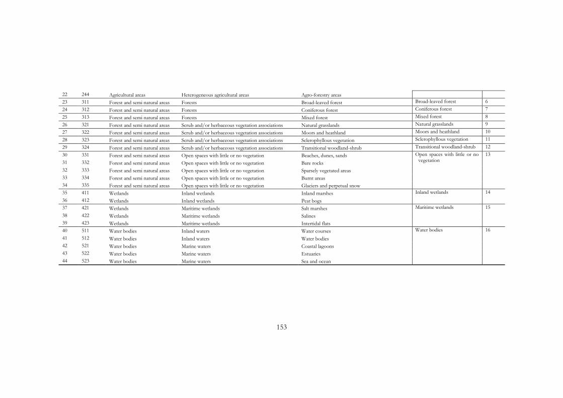
153

22 244 Agricultural areas Heterogeneous agricultural areas Agro-forestry areas 23 311 Forest and semi natural areas Forests Broad-leaved forest Broad-leaved forest 6 24 312 Forest and semi natural areas Forests Coniferous forest Coniferous forest 7 25 313 Forest and semi natural areas Forests Mixed forest Mixed forest 8 26 321 Forest and semi natural areas Scrub and/or herbaceous vegetation associations Natural grasslands Natural grasslands 9 27 322 Forest and semi natural areas Scrub and/or herbaceous vegetation associations Moors and heathland Moors and heathland 10 28 323 Forest and semi natural areas Scrub and/or herbaceous vegetation associations Sclerophyllous vegetation Sclerophyllous vegetation 11 29 324 Forest and semi natural areas Scrub and/or herbaceous vegetation associations Transitional woodland-shrub Transitional woodland-shrub 12 30 331 Forest and semi natural areas Open spaces with little or no vegetation Beaches, dunes, sands Open spaces with little or no

vegetation 13

31 332 Forest and semi natural areas Open spaces with little or no vegetation Bare rocks 32 333 Forest and semi natural areas Open spaces with little or no vegetation Sparsely vegetated areas 33 334 Forest and semi natural areas Open spaces with little or no vegetation Burnt areas 34 335 Forest and semi natural areas Open spaces with little or no vegetation Glaciers and perpetual snow 35 411 Wetlands Inland wetlands Inland marshes Inland wetlands 14 36 412 Wetlands Inland wetlands Peat bogs 37 421 Wetlands Maritime wetlands Salt marshes Maritime wetlands 15 38 422 Wetlands Maritime wetlands Salines 39 423 Wetlands Maritime wetlands Intertidal flats 40 511 Water bodies Inland waters Water courses Water bodies 16 41 512 Water bodies Inland waters Water bodies 42 521 Water bodies Marine waters Coastal lagoons 43 522 Water bodies Marine waters Estuaries 44 523 Water bodies Marine waters Sea and ocean

154

APPENDIX C SUMMARY TABLE OF THE MEAN PREDICTED OC STOCKS FOR THE SAMPLING DEPTH (20CM) WITH THE LOWER AND

UPPER LIMITS OF THE 95% CONFIDENCE INTERVAL. PREDICTIONS ARE

GIVEN FOR MINERAL VS. ORGANIC SOILS PER LAND COVER CLASS AND

WITHIN COUNTRIES

Country Land cover Soil Lower limit CI95

Mean stock

Upper limit CI95

AT bareland MIN 3.391 5.901 8.782 AT bareland ORG 0.643 0.733 0.832 AT cropland MIN 58.364 63.971 70.961 AT perm. crops MIN 6.814 8.793 11.767 AT grassland MIN 157.877 187.187 237.039 AT grassland ORG 2.071 2.152 2.243 AT shrubland MIN 21.739 23.751 25.897 AT shrubland ORG 0.314 0.344 0.375 AT woodland MIN 329.302 417.233 551.920 AT woodland ORG 100.804 102.450 103.959 AT wetlands ORG 4.368 4.529 4.676 BE bareland MIN 1.980 2.504 3.087 BE cropland MIN 30.960 34.601 38.790 BE perm. crops MIN 2.086 2.827 3.794 BE grassland MIN 89.664 99.070 109.738 BE grassland ORG 0.357 0.371 0.387 BE shrubland MIN 2.238 2.518 2.828 BE woodland MIN 58.749 67.611 77.141 BE woodland ORG 47.698 48.494 49.217 BE wetlands ORG 0.516 0.535 0.553 CZ bareland MIN 3.113 3.867 4.725 CZ cropland MIN 96.345 104.540 114.309 CZ perm. crops MIN 8.900 11.152 14.135 CZ grassland MIN 93.707 104.541 116.521 CZ shrubland MIN 4.064 4.565 5.141 CZ woodland MIN 260.959 298.194 343.406 CZ woodland ORG 3.210 3.260 3.309 CZ wetlands ORG 2.838 2.944 3.041

155

DE bareland MIN 11.593 15.041 18.971 DE bareland ORG 5.298 6.089 6.922 DE cropland MIN 450.517 498.986 559.029 DE cropland ORG 1.773 1.928 2.094 DE perm. crops MIN 29.541 36.965 46.373 DE grassland MIN 603.469 669.807 744.383 DE grassland ORG 123.006 128.101 133.590 DE shrubland MIN 23.366 25.966 28.799 DE shrubland ORG 2.346 2.572 2.806 DE woodland MIN 979.523 1116.115 1279.741 DE woodland ORG 423.511 430.458 436.918 DE wetlands ORG 19.875 20.615 21.285 DK bareland MIN 1.245 1.525 1.861 DK bareland ORG 2.214 2.550 2.890 DK cropland MIN 109.715 122.746 140.553 DK cropland ORG 2.369 2.581 2.807 DK perm. crops MIN 0.276 0.427 0.689 DK grassland MIN 49.743 58.114 67.046 DK grassland ORG 95.036 98.911 103.125 DK shrubland MIN 2.029 2.269 2.522 DK shrubland ORG 9.355 10.271 11.200 DK woodland MIN 8.002 9.111 10.530 DK woodland ORG 131.964 134.162 136.179 DK wetlands ORG 4.442 4.607 4.756 EE bareland MIN 0.915 1.157 1.446 EE bareland ORG 4.701 5.421 6.140 EE cropland MIN 27.573 30.282 33.672 EE cropland ORG 5.724 6.267 6.827 EE perm. crops MIN 0.059 0.255 0.483 EE grassland MIN 38.192 42.992 48.402 EE grassland ORG 71.855 74.767 77.944 EE shrubland MIN 6.016 6.817 7.755 EE shrubland ORG 7.179 7.885 8.603 EE woodland MIN 0.737 0.811 0.893 EE woodland ORG 460.075 467.679 474.710 EE wetlands ORG 35.619 36.940 38.134 ES bareland MIN 50.859 84.520 120.771

156

ES cropland MIN 283.815 335.323 393.096 ES perm. crops MIN 152.342 185.749 230.142 ES grassland MIN 352.092 421.706 509.978 ES grassland ORG 1.022 1.063 1.110 ES shrubland MIN 355.272 422.690 496.622 ES shrubland ORG 0.954 1.044 1.135 ES woodland MIN 610.163 774.564 974.778 ES woodland ORG 70.600 71.751 72.837 ES wetlands ORG 0.238 0.246 0.254 FI bareland MIN 1.093 1.450 1.872 FI bareland ORG 78.271 90.082 101.917 FI cropland MIN 211.998 251.011 302.629 FI cropland ORG 74.308 81.322 88.632 FI perm. crops MIN 0.074 0.413 0.857 FI grassland MIN 3.060 3.839 4.914 FI grassland ORG 308.539 320.983 334.640 FI shrubland MIN 0.149 0.179 0.215 FI shrubland ORG 408.446 448.388 488.499 FI woodland ORG 4178.990 4248.013 4311.878 FI wetlands ORG 270.926 280.975 290.061 FR bareland MIN 24.112 37.153 51.553 FR cropland MIN 663.319 735.057 819.554 FR perm. crops MIN 55.789 70.734 97.919 FR grassland MIN 1186.318 1325.263 1488.549 FR grassland ORG 2.860 2.976 3.106 FR shrubland MIN 207.480 231.262 255.432 FR shrubland ORG 0.372 0.408 0.444 FR woodland MIN 1476.284 1727.480 2041.793 FR woodland ORG 73.882 75.070 76.206 FR wetlands ORG 9.070 9.407 9.715 GR bareland MIN 6.622 12.795 19.614 GR cropland MIN 48.121 56.438 65.712 GR perm. crops MIN 41.667 52.383 67.394 GR grassland MIN 62.215 79.687 105.805 GR shrubland MIN 151.087 171.844 192.247 GR woodland MIN 193.937 262.037 373.826 GR woodland ORG 0.683 0.694 0.704

157

GR wetlands ORG 0.252 0.260 0.270 HU bareland MIN 2.028 2.518 3.062 HU cropland MIN 153.782 171.572 188.874 HU perm. crops MIN 6.856 8.846 11.082 HU grassland MIN 95.813 107.726 122.659 HU shrubland MIN 13.902 15.375 16.996 HU woodland MIN 99.155 113.351 129.470 HU woodland ORG 3.277 3.321 3.374 HU wetlands ORG 10.502 10.886 11.254 IE bareland MIN 0.966 1.326 1.740 IE bareland ORG 5.943 6.831 7.731 IE cropland MIN 15.081 18.086 21.719 IE cropland ORG 1.742 1.900 2.067 IE grassland MIN 172.820 201.784 235.260 IE grassland ORG 577.566 601.133 626.822 IE shrubland MIN 3.207 3.537 3.900 IE shrubland ORG 78.856 86.565 94.248 IE woodland MIN 0.622 0.872 1.370 IE woodland ORG 148.841 151.302 153.576 IE wetlands ORG 56.725 58.830 60.733 IT bareland MIN 16.568 27.228 38.741 IT bareland ORG 0.329 0.371 0.424 IT cropland MIN 230.943 263.238 303.535 IT perm. crops MIN 131.564 165.183 208.492 IT grassland MIN 248.727 301.504 383.066 IT shrubland MIN 122.616 141.043 159.631 IT woodland MIN 560.700 741.961 1042.326 IT woodland ORG 41.334 41.999 42.623 IT wetlands ORG 1.774 1.839 1.901 LT bareland MIN 2.967 3.637 4.449 LT bareland ORG 0.319 0.366 0.414 LT cropland MIN 68.986 75.510 83.860 LT cropland ORG 0.337 0.367 0.399 LT perm. crops MIN 0.440 0.968 1.361 LT grassland MIN 115.980 129.537 143.371 LT grassland ORG 19.538 20.336 21.187 LT shrubland MIN 7.367 8.264 9.242

158

LT shrubland ORG 3.821 4.190 4.576 LT woodland MIN 38.880 45.022 52.098 LT woodland ORG 340.110 345.827 350.993 LT wetlands ORG 4.490 4.657 4.808 LU bareland MIN 0.218 0.265 0.318 LU cropland MIN 1.989 2.301 2.561 LU perm. crops MIN 0.298 0.347 0.417 LU grassland MIN 6.334 6.954 7.675 LU shrubland MIN 0.158 0.172 0.185 LU woodland MIN 7.511 8.444 9.453 LU woodland ORG 1.354 1.375 1.397 LV bareland MIN 3.243 4.021 4.958 LV bareland ORG 3.793 4.353 4.935 LV cropland MIN 36.925 40.512 45.540 LV cropland ORG 0.674 0.736 0.801 LV perm. crops MIN 0.326 0.968 1.542 LV grassland MIN 87.871 98.771 110.757 LV grassland ORG 55.339 57.585 60.016 LV shrubland MIN 16.854 18.855 21.189 LV shrubland ORG 16.026 17.595 19.203 LV woodland MIN 21.668 24.632 27.861 LV woodland ORG 560.272 569.537 578.093 LV wetlands ORG 26.472 27.455 28.343 NL bareland MIN 2.159 2.810 3.514 NL bareland ORG 0.726 0.833 0.947 NL cropland MIN 40.943 47.391 55.509 NL perm. crops MIN 3.250 4.599 6.333 NL grassland MIN 129.443 142.895 158.923 NL grassland ORG 66.870 69.692 72.695 NL shrubland MIN 5.927 6.587 7.251 NL shrubland ORG 1.094 1.199 1.311 NL woodland MIN 7.893 9.070 10.358 NL woodland ORG 86.756 88.217 89.547 NL wetlands ORG 2.963 3.073 3.173 PL bareland MIN 15.307 18.807 22.930 PL bareland ORG 1.259 1.442 1.634 PL cropland MIN 338.396 373.496 413.352

159

PL perm. crops MIN 13.109 17.090 21.286 PL grassland MIN 430.838 483.028 540.288 PL grassland ORG 83.824 87.446 91.054 PL shrubland MIN 25.069 28.302 31.907 PL shrubland ORG 5.153 5.635 6.168 PL woodland MIN 496.481 560.741 638.536 PL woodland ORG 453.255 460.703 467.675 PL wetlands ORG 17.778 18.440 19.039 PT bareland MIN 12.353 19.095 26.522 PT cropland MIN 21.214 26.646 33.493 PT perm. crops MIN 26.652 36.204 49.283 PT grassland MIN 58.410 72.084 87.801 PT shrubland MIN 109.028 125.426 141.615 PT shrubland ORG 0.317 0.347 0.378 PT woodland MIN 197.836 235.637 281.845 PT woodland ORG 1.648 1.675 1.700 PT wetlands ORG 0.482 0.505 0.519 SE bareland MIN 9.045 12.145 15.770 SE bareland ORG 170.391 195.515 221.573 SE cropland MIN 96.568 109.663 127.772 SE cropland ORG 5.396 5.895 6.416 SE perm. crops MIN 0.206 0.326 0.483 SE grassland MIN 42.662 51.310 62.102 SE grassland ORG 369.147 384.140 400.485 SE shrubland MIN 22.918 27.320 32.078 SE shrubland ORG 678.877 745.072 812.209 SE woodland MIN 1.989 2.236 2.515 SE woodland ORG 5747.807 5842.140 5929.863 SE wetlands ORG 430.284 446.245 460.676 SI bareland MIN 0.819 1.460 2.202 SI bareland ORG 0.316 0.359 0.408 SI cropland MIN 6.371 7.252 8.283 SI perm. crops MIN 1.998 2.763 4.089 SI grassland MIN 30.862 35.411 41.099 SI grassland ORG 0.340 0.353 0.368 SI shrubland MIN 5.889 6.443 7.039 SI woodland MIN 98.948 118.684 142.577

160

SI woodland ORG 45.582 46.338 47.016 SI wetlands ORG 0.477 0.495 0.511 SK bareland MIN 1.133 1.521 1.955 SK cropland MIN 45.113 49.694 54.569 SK perm. crops MIN 3.099 3.778 4.640 SK grassland MIN 48.810 55.693 64.372 SK shrubland MIN 15.752 17.326 18.979 SK woodland MIN 131.087 153.768 181.728 SK woodland ORG 22.611 22.967 23.313 SK wetlands ORG 0.468 0.485 0.501 UK bareland MIN 8.746 12.031 15.881 UK bareland ORG 49.829 57.344 64.803 UK cropland MIN 248.645 283.458 327.460 UK cropland ORG 4.647 5.073 5.520 UK perm. crops MIN 1.573 6.668 120.773 UK grassland MIN 574.955 719.223 928.014 UK grassland ORG 1092.634 1136.970 1185.518 UK shrubland MIN 40.486 45.142 49.924 UK shrubland ORG 429.861 471.861 513.732 UK woodland MIN 84.899 108.326 143.822 UK woodland ORG 542.462 551.438 559.737 UK wetlands ORG 64.502 66.895 69.058