SIAM J. SCI. COMPUT. c© 2017 Society for Industrial and Applied MathematicsVol. 39, No. 1, pp. B29–B52

COMBINING DEFLATION AND NESTED ITERATION FORCOMPUTING MULTIPLE SOLUTIONS OF NONLINEAR

VARIATIONAL PROBLEMS∗

J. H. ADLER† , D. B. EMERSON† , P. E. FARRELL‡ , AND S. P. MACLACHLAN§

Abstract. Many physical systems support multiple equilibrium states that enable their usein modern science and engineering applications. Having the ability to reliably compute such statesfacilitates more accurate physical analysis and understanding of experimental behavior. This paperadapts and extends a deflation technique for the computation of multiple distinct solutions in thecontext of nonlinear systems and applies the method to the modeling of equilibrium configurationsof nematic and cholesteric liquid crystals. In particular, the deflation approach is interwoven withnested iteration, creating an efficient and effective method that further enables the discovery ofdistinct solutions. The combined methodology is applied as part of an overall free-energy variationalapproach within the framework of optimization of a functional with constraints imposed via Lagrangemultipliers. A key feature in the combined algorithm is the reuse of effective preconditioners designedfor the undeflated systems within the Newton iteration for the deflated systems. Four numericalexperiments are performed, demonstrating the efficacy and accuracy of the algorithm in detectingimportant physical phenomena, including bifurcation and disclination behaviors.

Key words. liquid crystal simulation, deflation methods, energy optimization, nested iteration,distinct solutions

AMS subject classifications. 76A15, 65N30, 49M15, 65N22, 65N55

DOI. 10.1137/16M1058728

1. Introduction. It is well known that many systems of nonlinear partial dif-ferential equations (PDEs) permit multiple solutions. The numerical solution of suchsystems is of key interest in many settings, particularly for bistable and multistablephysical systems, where understanding the solution set is crucial to the design andoptimization of physical devices. In [22], a deflation methodology was proposed toenable the sequential discovery of distinct solutions to nonlinear differential equations,based on modifying the typical Newton iteration applied to their discretizations. Theresulting iteration is demonstrated therein to be efficient, with roughly the sameamount of computational effort required to find each additional solution, and to suc-cessfully discover numerous solutions to classical problems, such as an Allen–Cahnequation and the Navier–Stokes equations. In this paper, we adapt and expand thedeflation methodology by combining it with nested iteration (NI) [4, 6, 12, 37, 44], apowerful approach to reducing computational cost in the solution of nonlinear PDEs.To demonstrate the performance of the resulting algorithm, we apply it to models in

∗Submitted to the journal’s Computational Methods in Science and Engineering section Janu-ary 27, 2016; accepted for publication (in revised form) October 14, 2016; published electronicallyJanuary 24, 2017.

http://www.siam.org/journals/sisc/39-1/M105872.htmlFunding: The third author’s work was funded by EPSRC grants EP/K030930/1 and

EP/M011151/1 and a Center of Excellence grant from the Research Council of Norway to the Centerfor Biomedical Computing at Simula Research Laboratory. The fourth author’s work was partiallysupported by an NSERC Discovery Grant.

†Department of Mathematics, Tufts University, Medford, MA 02155 (james.adler@tufts.edu,david.emerson@tufts.edu).

‡Mathematical Institute, University of Oxford, Oxford OX2 6GG, United Kingdom (patrick.farrell@maths.ox.ac.uk).

§Department of Mathematics and Statistics, Memorial University of Newfoundland, St. John’s,Newfoundland and Labrador A1C 5S7, Canada (smaclachlan@mun.ca).

B29

B30 ADLER, EMERSON, FARRELL, AND MACLACHLAN

liquid crystal theory, as an example of the coupled systems that arise in multiphysicssimulation.

In general, the deflation methodology sequentially modifies the nonlinear problemto be solved by eliminating previously known solutions from consideration. This al-lows for successive discovery of distinct solutions to the nonlinear system. In practice,the deflation approach is highly effective in locating several distinct solutions. Here,we examine the method’s performance in the context of constrained variational formu-lations arising in free-energy optimization. Such a framework is central to simulatingvarious multiphysics applications, such as liquid crystals (addressed here), ferromag-netics [32], and magnetohydrodynamics [29]. In the context of these types of problems,multiple local extrema and saddle-point solutions satisfying the given constraints maybe present. Locating distinct solutions thus both reveals configurations with phys-ical relevance, such as defect arrangements in the case of liquid crystals consideredhere, and facilitates computing global extrema with a higher level of confidence thanotherwise possible.

The success of the deflation methodology relies on the efficiency of the underlyingnonlinear and linear solvers. For the linear solvers, the deflation methodology isnaturally attractive, as it allows for the preservation of the sparsity patterns seenin typical finite-element simulations as well as the use of existing fast solvers forthe linearized systems. To address efficiency of the underlying nonlinear solvers, inthis paper, we extend the deflation technique by integrating it with an NI approach,as is commonly done to improve that efficiency. NI is an important tool for theefficient numerical solution of nonlinear PDEs [44]. The system is first solved on acoarse level, where computation is cheap. A series of refinement steps are then taken,interpolating the coarse-grid solution to a finer mesh and using this as an initial guessfor the fine-grid problem. A key advantage is that these interpolated approximationsare typically very good initial guesses for Newton’s method on the finer grids, so veryfew iterations are needed on fine levels, where computation is expensive. NI strategieshave been applied successfully to a variety of applications that involve coupled physics(e.g., [4, 6, 12, 37]).

To demonstrate the utility of deflation combined with NI and multigrid, we con-sider a variety of static liquid crystal problems. The presence of multiple solutionsto liquid crystal systems is well known and central to their use in many industries,including modern display technology. Numerical simulations of liquid crystal con-figurations are used to examine theory, explore new physical phenomena [1, 7], andoptimize device performance. For static liquid crystal structures, the associated sys-tem of PDEs, known as the equilibrium equations [20, 46], permits multiple solutions,even under relatively mild complexity [18]. Further, multiple locally optimal config-urations and saddle-point structures may exist for the energy formulation. Thus, inthis paper, we incorporate deflation into the constrained optimization approach pre-viously developed in [1, 2]. This yields an adaptable and efficient method that enablesthe discovery of distinct solutions for such problems.

This paper is organized as follows. The deflation technique is discussed and de-rived in the context of variational optimization formulations in section 2. The combi-nation of deflation with NI and the integration of existing (multigrid) preconditionersare also examined in this section. The liquid crystal energy model and existing mini-mization approach without deflation are summarized in section 3. In sections 4 and5, the implementation of the algorithm is outlined and four numerical experimentsare performed. Finally, section 6 provides some concluding remarks and a discussionof future work.

DEFLATION AND NESTED ITERATION B31

2. Deflation methodology. A standard but unsystematic approach to com-puting distinct solutions for nonlinear problems with several solutions is the use ofnumerous initial guesses as part of an overarching Newton-type scheme, known asmultistart methods [38]. In this section, we adapt the deflation technique first pro-posed in [22] as a more effective and systematic alternative. The essential idea is tocast the constrained minimization problem as the solution of the associated optimalityconditions and then to repeatedly modify the nonlinear problem to eliminate knownsolutions as they are found.

First, consider a general variational problem, posed as minu∈U L(u), where u ∈ Ugathers the continuum variables to be solved for, and L : U → R is a nonlinear func-tional. Then, the Euler–Lagrange equations are naturally given by the first variation,such that

A(u;v) := Lu[v] = 0 ∀v ∈ U,(2.1)

where the Gateaux derivative, Lu[v], is evaluated at u in the direction v (whenimposing Dirichlet boundary conditions on u, we may also take v in U0, correspondingto the test space appropriately adjusted to functions that take value 0 on the Dirichletboundary). Note that A : U × U → R is linear in its second argument and can bewritten as A(u;v) = 〈f(u),v〉, where f : U → U∗, and U∗ is the dual space of U .

We think of the nonlinear equation to be solved as either the variational formin (2.1) or the “residual” equation f(u) = 0 (noting that this equality is taken tobe in U∗), and we note that it may have multiple solutions, even when there is aunique global minimum to the original variational problem. The question of whethercomputed solutions to the Euler–Lagrange equations represent global minima or onlylocal minima (or maxima or saddle points) is often difficult to answer with certainty.The deflation technique presented in this section systematically promotes the discov-ery of numerous solutions, revealing stable and unstable local minima and increasingthe probability of the identification of a global minimizer.

Suppose one solution, r, to (2.1) has been found. We construct a deflated residual,

g(u) =Mp,α(u; r)f(u),(2.2)

where Mp,α is the shifted deflation operator,

Mp,α(u; r) =

(1

‖u− r‖pU+ α

)I.

Here α ≥ 0 is a scalar shift, p ∈ [1,∞) is the deflation exponent, and I is the identityoperator on U∗. Thus, for fixed u, r ∈ U , the deflation operator Mp,α(u; r) is simplya scaled identity operator in U∗. Applying the deflation operator to the residual fensures that Newton’s method applied to the resulting variational system will notconverge to r under mild regularity conditions on the solution [22]. In the context of(2.1), the resulting deflated variational operator is given by

G(u;v) = 〈Mp,α(u; r)f(u),v〉 =⟨(

1

‖u− r‖pU+ α

)f(u),v

⟩.

This produces the deflated variational problem

G(u;v) = 0 ∀v ∈ U.(2.3)

B32 ADLER, EMERSON, FARRELL, AND MACLACHLAN

A nonzero shift, α, is applied so that the deflated residual does not tend to zero as‖u − r‖U becomes arbitrarily large; see [22]. While the method is generally robustwith respect to parameter choice, there are situations where additional performanceimprovements are attainable for certain selections of p and α.

For brevity, we suppress the semicolon notation in the variational operators exceptwhen necessary for clarity and denote η(u) = ( 1

‖u−r‖pU+ α). Note that the deflated

residual g(u) = η(u)f(u) is also nonlinear. Thus, we consider its solution via Newton’smethod, linearizing g(u) = 0 around an approximate solution, uk, and solving for anupdate δu that satisfies

〈g(uk) + g′(uk)δu,v〉 = 0 ∀v ∈ U,

where g′(uk) is the Frechet derivative of g(u) evaluated at uk. Applying the productrule to g(u), we have that

g′(uk) = η(uk)f′(uk) + f(uk)η

′(uk),

where f ′(uk) and η′(uk) are the Frechet derivatives of f and η, respectively, evaluated

at uk. We note that g′(uk) and f ′(uk) become the standard Jacobians of g and f whendiscretized, as discussed below. With this, we now discretize and solve the linearizedvariational problem: find δu such that

〈g′(uk)δu,v〉 = −〈g(uk),v〉 ∀v ∈ U.(2.4)

This is used to compute the updated approximation uk+1 = uk + ωδu with a steplength ω ∈ R.

2.1. Deflated linear systems. A strategy for constructing effective precondi-tioners for the deflated system based on existing preconditioners for the undeflatedmatrices and computing their actions in a matrix-free fashion is presented in [22].This section provides a general framework for efficient reuse of good preconditionersdesigned for the original Newton linearizations, which is particularly necessary in thecontext of mixed finite-element discretizations of multiphysics problems. In sections4 and 5, we utilize this approach to apply monolithic multigrid preconditioners, asdeveloped in [1, 3], to solve for the updates in (2.4).

Let F (uk) and G(uk) denote the vectors corresponding to discretizations of f(uk)and g(uk), respectively, and let d(uk) be the discretization vector corresponding tothe Frechet derivative of η. Let JG(uk) and JF (uk) indicate the discretized Jacobiansof the deflated and undeflated systems, respectively. Then,

JG(uk) = η(uk)JF (uk) + F (uk)d(uk)T .(2.5)

As defined, JG(uk) is composed of a rank-one update to JF (uk). Thus, JG(uk) isgenerally dense, even if JF (uk) is not, and explicit construction and computation withthe matrix is prohibitively expensive. Throughout the remainder of the paper, exceptwhen necessary for clarity, we neglect the dependence on uk in the notation.

Considering JG = (ηJF +FdT ) and applying the Sherman–Morrison formula [30]gives

J−1G = (ηJF + FdT )−1 =

J−1F

η−

1η2 J

−1F FdT J−1

F

1 + 1ηd

TJ−1F F

.(2.6)

DEFLATION AND NESTED ITERATION B33

Using (2.6) to compute the discretized update vector corresponding to (2.4) produces

−J−1G G = −J

−1F G

η+

1η2 J

−1F FdTJ−1

F G

1 + 1ηd

T J−1F F

= −J−1F F +

1ηJ

−1F FdTJ−1

F F

1 + 1η · dT J−1

F F

= −(1−

1η · dT J−1

F F

1 + 1η · dTJ−1

F F

)J−1F F.

Note that J−1F F corresponds to assembling and solving the original undeflated prob-

lem and dT J−1F F is a dot product resulting in a scalar. Thus, solving the discrete form

of the deflation system in (2.4) is reduced to a single solve with the original sparsesystem, one dot product, one vector scaling, and a few scalar operations. Therefore,any preconditioner developed to effectively solve the undeflated Newton systems canbe directly applied to the deflated systems that arise in (2.4), yielding an efficientalgorithm for computing the deflated updates.

2.2. Multiple deflation. Thus far, the class of deflation operators consideredfocuses on deflation with one known solution, r. In this section, we briefly discussextending the deflation procedure to treat a family of known solutions r1, r2, . . . , rm.With several known solutions, the multiple deflation operator is the product of thesingle deflation operators for each individual solution such that

Mp,α(u; r1, r2, . . . , rm) =

m∏i=1

Mp,α(u; ri).

This modifies the action of Mp,α(u; r1, r2, . . . , rm) on f(u) such that

G(u;v) =⟨

m∏i=1

Mp;α(u, ri)f(u),v

⟩=

⟨(m∏i=1

(1

‖u− ri‖pU+ α

))f(u),v

⟩,

which we recognize, as in the case of single deflation, to be a scaling of the resid-ual with the form g(u) = η(u)f(u). This deflated system remains nonlinear, andcorresponding linearizations are derived to compute distinct solutions satisfying thefirst-order optimality conditions. As with the single deflation linearization, the dis-cretized multiple deflation Jacobian, JG, is composed of a rank-one update to JF asin (2.5), though d(uk) is now more complicated than the single deflation case. Aprocess similar to that applied in the single deflation case reveals an analogous resultfor computation of solutions to the discretized, deflated linearizations and yields sim-ilar results enabling the application of preexisting preconditioners to linear systemssubject to deflation over several known solutions. Each of the simulations to followemploys multisolution deflation operators as distinct solutions are discovered.

2.3. Interaction with nested iteration. To improve the efficiency of the over-all algorithm, we propose here directly integrating the deflation methodology with NI.The process begins on a coarse grid, with a small number of degrees of freedom, fol-lowed by a series of refinements until the final desired mesh resolution is obtained.On each refinement level, a combination of continued iteration on known solutionsfollowed by applying deflation to uncover additional solutions is performed. The gen-eral numerical flow is detailed below in Algorithm 1. The algorithm has four mainstages. The outermost phase is an NI hierarchy that has proven highly effective inreducing computational work for systems of nonlinear PDEs discretized by appropri-ate finite-element methods [2, 4, 5, 6, 12, 37, 44]. On each mesh, the algorithm first

B34 ADLER, EMERSON, FARRELL, AND MACLACHLAN

performs (undeflated) Newton iterations on interpolated versions of solutions foundon the previous, coarser mesh, termed the continuation list in Algorithm 1, to fur-ther resolve the solution features on the finer mesh. On the coarsest mesh, one ormore simple initial guesses are taken in place of the interpolated information. Thisprocedure is followed by a solution discovery stage where all known solutions are de-flated and new solutions are sought. Each deflation solve begins with an initial guesstaken from a list of (possibly several) initialization vectors. Newton iterations areperformed until a convergence tolerance is reached for a new solution (added to thesolution list in Algorithm 1) or a maximum number of Newton iterations have beenperformed. For both the deflated and undeflated Newton iterations, the convergencestopping criterion on a given level is based on a set tolerance for an approximation’sconformance to the first-order optimality conditions in the standard Euclidean l2-norm. Throughout the numerical results below (see sections 4 and 5), this toleranceis held at 10−4. Since this is imposed in the discrete l2-norm, this translates to anincreasingly tighter constraint on the error in the continuum L2-norm as the meshis refined. For each deflated Newton iteration, the matrix-free approach outlined insection 2.1 can be used, so that the efficiency of the linear iterations depends onlyon that of the underlying preconditioner (or other solver) for the undeflated system.Finally, the known solution approximations are interpolated to a finer grid to formthe continuation list there. In the current implementation, these finer grids representsuccessive uniform refinements of the initial coarse grid.

The blending of NI and deflation outlined above has a number of advantages aboveand beyond efficiency. Certain solutions are more readily detectable through deflationprocesses on both coarser and finer meshes, as observed in the numerical results tofollow. Moreover, the algorithm allows for varying and adaptive initial guesses. Thatis, in addition to a static set of initial guesses for the deflation solves on each grid,sets of initial guesses may be constructed from transformations of known or newlydiscovered solutions throughout the NI and deflation process. Constructing strategiesfor adaptive generation of initial guesses will be the subject of future work.

2.4. Newton stepping. A form of damped Newton stepping is applied for boththe undeflated and deflated updates such that the next iterates are given by

uk+1 = uk + ωδu,

where 0 < ω ≤ 1 is a damping parameter. For the undeflated solves, we take ω = ω1

on the coarsest grid and increase its value by Δ1 at each level of refinement to amaximum value of 1. With the deflated systems, we take ω = ω2 on the coarsest gridand decrease its value by Δ2 at each level of refinement to a minimum value of 0.2.This strategy aims at improving convergence for both types of iterations. For the un-deflated solves, the damping parameter is increased on each grid as confidence in theNewton convergence increases for more finely resolved solutions. On the other hand,in numerical experiments, some convergence issues have been observed for deflationiterations beginning with poor initial guesses on fine meshes. Hence, the decreasingdamping parameter increases the likelihood of convergence on finer grids within thedeflation iterations. While more advanced step selection methods, such as trust re-gions [5, 10], are well established, we experimentally observed that using trust regionsduring the deflation phase of the algorithm hindered the method’s ability to discovernew basins of attraction, thereby limiting the number of unique solutions found.Specifically, with the application of the deflation operator, additional nonlinearity isintroduced to the variational system under consideration. This generally results in

DEFLATION AND NESTED ITERATION B35

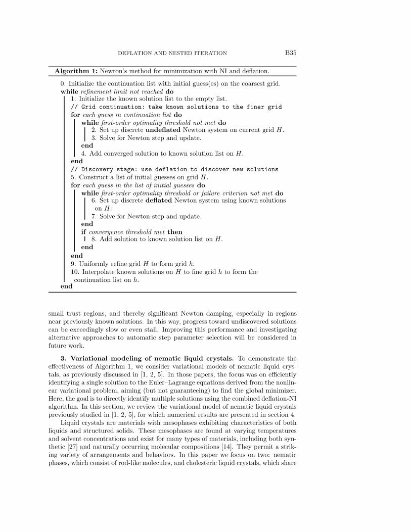
Algorithm 1: Newton’s method for minimization with NI and deflation.

0. Initialize the continuation list with initial guess(es) on the coarsest grid.while refinement limit not reached do

1. Initialize the known solution list to the empty list.// Grid continuation: take known solutions to the finer grid

for each guess in continuation list dowhile first-order optimality threshold not met do

2. Set up discrete undeflated Newton system on current grid H .3. Solve for Newton step and update.

end4. Add converged solution to known solution list on H .

end// Discovery stage: use deflation to discover new solutions

5. Construct a list of initial guesses on grid H .for each guess in the list of initial guesses do

while first-order optimality threshold or failure criterion not met do6. Set up discrete deflated Newton system using known solutionson H .7. Solve for Newton step and update.

endif convergence threshold met then

8. Add solution to known solution list on H .end

end9. Uniformly refine grid H to form grid h.10. Interpolate known solutions on H to fine grid h to form thecontinuation list on h.

end

small trust regions, and thereby significant Newton damping, especially in regionsnear previously known solutions. In this way, progress toward undiscovered solutionscan be exceedingly slow or even stall. Improving this performance and investigatingalternative approaches to automatic step parameter selection will be considered infuture work.

3. Variational modeling of nematic liquid crystals. To demonstrate theeffectiveness of Algorithm 1, we consider variational models of nematic liquid crys-tals, as previously discussed in [1, 2, 5]. In those papers, the focus was on efficientlyidentifying a single solution to the Euler–Lagrange equations derived from the nonlin-ear variational problem, aiming (but not guaranteeing) to find the global minimizer.Here, the goal is to directly identify multiple solutions using the combined deflation-NIalgorithm. In this section, we review the variational model of nematic liquid crystalspreviously studied in [1, 2, 5], for which numerical results are presented in section 4.

Liquid crystals are materials with mesophases exhibiting characteristics of bothliquids and structured solids. These mesophases are found at varying temperaturesand solvent concentrations and exist for many types of materials, including both syn-thetic [27] and naturally occurring molecular compositions [14]. They permit a strik-ing variety of arrangements and behaviors. In this paper we focus on two: nematicphases, which consist of rod-like molecules, and cholesteric liquid crystals, which share

B36 ADLER, EMERSON, FARRELL, AND MACLACHLAN

many similarities with nematics but intrinsically prefer helical structures that admitless symmetry due to chiral preference. These types of liquid crystals self-assembleinto ordered structures characterized by a preferred average direction at each pointknown as the director. The director is described by a unit vector field at each pointand is denoted n(x, y, z) = (n1(x, y, z), n2(x, y, z), n3(x, y, z))

T . Along with their crys-talline self-structuring, liquid crystals demonstrate a number of important physicalphenomena including birefringence, electric coupling, and flexoelectric effects. Com-prehensive reviews of liquid crystal physics are found in [17, 46, 47]. These propertiesand others have led to many important discoveries and a diversity of applications(e.g., [33, 43, 48]).

3.1. Frank–Oseen free-energy model. While a number of models exist [16,40, 46], we consider the Frank–Oseen free-energy model for the computation of liquidcrystal equilibrium configurations [46, 47]. The complexity of the model and thenecessary nonlinear pointwise unit-length constraint have limited the availability ofanalytical solutions in the absence of significant simplifying assumptions. Recently, anumber of numerical methods [7, 26, 41, 42] have been proposed for the Frank–Oseenmodel. In [1, 2], an energy-minimization finite-element technique was developed thatallows accurate and efficient computational simulation of liquid crystal behavior. Thisapproach is presented here and combined with the deflation-NI methodology below.

The Frank–Oseen free-energy model characterizes the equilibrium free energy for adomain Ω by deformations of the nondimensional, unit-length director field, n. Liquidcrystals tend toward configurations exhibiting minimal free energy. Let Ki, i = 1, 2, 3,be the Frank constants [23] with Ki ≥ 0 [21]. Here, we consider the case that eachKi �= 0. These constants are often anisotropic (i.e., K1 �= K2 �= K3), vary withliquid crystal type, and play important roles in physical phenomena [8, 34]. In orderto properly formulate the Lagrangian below, a nondimensionalization, introducedin [5], using a characteristic length scale, σ, a characteristic Frank constant, K, and acharacteristic voltage, φ0 > 0, is applied so that the entire expression is dimensionless.

We denote the classical L2(Ω) inner product and norm as 〈·, ·〉0 and ‖ · ‖0, respec-tively, for both scalar and vector quantities. Throughout this paper, we assume thepresence of Dirichlet boundary conditions or mixed Dirichlet and periodic boundaryconditions on a rectangular domain and, therefore, utilize the null Lagrangian simpli-fication discussed in [1, 46]. Hence, including the possibility of external electric fields(but not flexoelectric effects), the Frank–Oseen free energy for nematics is written as

F(n, φ) = K1‖∇ · n‖20 +K3〈Z∇× n,∇× n〉0 − ε0ε⊥〈∇φ,∇φ〉0− ε0εa〈n · ∇φ,n · ∇φ〉0,(3.1)

where φ is an electric potential, ε0 denotes the permittivity of free space, and thedimensionless constants ε⊥ and εa are the perpendicular dielectric permittivity anddielectric anisotropy of the liquid crystal, respectively. Finally, Z = κn ⊗ n + (I −n ⊗ n) = I − (1 − κ)n ⊗ n is a dimensionless tensor, where κ = K2/K3. Note thatif κ = 1, Z reduces to the identity. In the existing literature (including [1, 2]), thefunctional in (3.1) is typically scaled by a factor of 1

2 ; while we derive the expressionsbelow without this scaling, we include it in the free energies reported in sections 4and 5 for consistency with other papers.

The director field is subject to a local unit-length constraint such that n ·n = 1 ateach point throughout the domain. In [5], numerical evidence indicates that imposingthis constraint with Lagrange multipliers is an accurate and highly efficient approach,particularly in comparison to penalty or renormalization formulations. Note that in

DEFLATION AND NESTED ITERATION B37

the case that K1 = K2 = K3 with no electric field, a linear free-energy functional isobtained. Coupled with the unit-length constraint, the minimization corresponds toa weak harmonic mapping problem. Existence and uniqueness theory for this type ofproblem has been analyzed in [31].

Throughout this paper, we will make use of the spaces H(div,Ω) = {w ∈(L2(Ω)

)3: ∇ · w ∈ L2(Ω)} and H(curl,Ω) = {w ∈ (L2(Ω)

)3: ∇ × w ∈ (L2(Ω)

)3}.As in [1], define

HDC(Ω) = {w ∈ H(div,Ω) ∩H(curl,Ω) : B(w) = g},with norm ‖w‖2DC = ‖w‖20+‖∇·w‖20+‖∇×w‖20 and appropriate boundary conditionsB(w) = g. Here, we assume that g satisfies appropriate compatibility conditions forthe operator B. For example, if B represents full Dirichlet boundary conditions and Ωhas a Lipschitz continuous boundary, it is assumed that g ∈ H

12 (∂Ω)3 [28]. Further,

let HDC0 (Ω) = {w ∈ H(div,Ω)∩H(curl,Ω) : B(w) = 0}. Note that if Ω is a Lipschitz

domain and B imposes full Dirichlet boundary conditions on all components of w,

then HDC0 (Ω) =

(H1

0 (Ω))3

[28, Lemma 2.5]. Denote

H1,g(Ω) = {f ∈ H1(Ω) : B1(f) = g},where H1(Ω) represents the classical Sobolev space with norm ‖ · ‖1 and B1(f) = gis an appropriate boundary condition expression for the electric potential, φ.

We define the Lagrangian as

L(n, φ, λ) = F(n, φ) +

∫Ω

λ(x)(n · n− 1) dV,

where L(n, φ, λ) has been nondimensionalized in the same fashion as the free-energyfunctional. To minimize the functional, first-order optimality conditions are derivedas

Ln[w] =∂

∂nL(n, φ, λ)[w] = 0 ∀w ∈ HDC

0 (Ω),(3.2)

Lφ[ψ] =∂

∂φL(n, φ, λ)[ψ] = 0 ∀ψ ∈ H1,0(Ω),(3.3)

Lλ[γ] =∂

∂λL(n, φ, λ)[γ] = 0 ∀γ ∈ L2(Ω),(3.4)

with A(n, φ, λ;w, ψ, γ) = Ln[w]+Lφ[ψ]+Lλ[γ] being the combined variational form.For the Frank–Oseen model in (3.1), these Gateaux derivatives are given by

Ln[w] = 2K1〈∇ · n,∇ ·w〉0 + 2K3〈Z∇× n,∇×w〉0+ 2(K2 −K3)〈n · ∇ × n,w · ∇ × n〉0− 2ε0εa〈n · ∇φ,w · ∇φ〉0 + 2

∫Ω

λ(n,w) dV = 0 ∀w ∈ HDC0 (Ω),

Lφ[ψ] = −2ε0ε⊥〈∇φ,∇ψ〉0 − 2ε0εa〈n · ∇φ,n · ∇ψ〉0 = 0 ∀ψ ∈ H1,0(Ω),

Lλ[γ] =

∫Ω

γ((n,n)− 1) dV = 0 ∀γ ∈ L2(Ω).

To express this problem in the general framework of section 2, we identify theproduct space U = HDC(Ω) ×H1,g(Ω) × L2(Ω) with associated norm ‖ · ‖U , and its

B38 ADLER, EMERSON, FARRELL, AND MACLACHLAN

subspace U0 = HDC0 (Ω)×H1,0(Ω)×L2(Ω). For any u ∈ U , we naturally identify u =

(n, φ, λ)T . The Euler–Lagrange equations above in (3.2)–(3.4) define the variationalform A : U × U0 → R termwise, giving the first variation as finding u ∈ U such thatA(u;v) = 0 for all v ∈ U0. Note that this variational system is nonlinear and, inmany cases, admits several distinct solutions. For example, the classical Freedericksztransition problem [24, 49], which is discussed in detail below, admits at least threesolutions to the first-order optimality conditions.

In [1, 2], Newton linearizations and a finite-element discretization are used tocompute solutions to this variational system. This linearization yields the Newtonupdate equations

JF (uk)[δu] =

⎡⎣ Lnn Lnφ Lnλ

Lφn Lφφ 0Lλn 0 0

⎤⎦⎡⎣ δnδφδλ

⎤⎦ = −

⎡⎣ Ln

Lφ

Lλ

⎤⎦ ,(3.5)

where each of the system components is evaluated at nk, φk, and λk, the currentapproximations for n, φ, and λ, and δn = nk+1 − nk, δφ = φk+1 − φk, and δλ =λk+1 − λk are the updates we seek to compute. Here, following the mixed finite-element formulation in [1, 2], we write JF as a matrix acting on the components of

δu = (δn, δφ, δλ)T, rather than in the more compact notation of section 2. For the

full Hessian computations, see Appendix A. In addition to enabling the constructionof the linearized system, deriving the components of the Hessian permits numericalstudy of the energetic stability of computed solutions. Techniques for such analysisare not developed here but are possible as a postprocessing step once equilibriumstates have been computed.

3.2. Discretization and multigrid preconditioning of the Jacobian sys-tem. For the test problems below, we consider a classical domain with two parallelsubstrates placed at unit distance apart. These substrates run parallel to the xz-planeand perpendicular to the y-axis. Further, we assume a slab-type domain such that nmay have a nonzero z-component, but ∂n

∂z = 0. Thus, for the numerical experimentsto follow, Ω = {(x, y) : 0 ≤ x, y ≤ 1}. In the first two experiments of section 4, peri-odic boundary conditions are applied at the left and right boundaries, and Dirichletconditions are enforced at the top and bottom of the domain. In the third experimentof the section, Dirichlet boundary conditions are applied for the entire boundary. Inall experiments, we use biquadratic finite elements to discretize components associ-ated with n and φ in the variational systems, while piecewise constants are used forthose related to λ. In each simulation, the algorithm begins on a uniform 8× 8 coarsemesh, ascending in uniform refinements to a 256×256 fine grid. This results in a totalof 1, 118, 212 degrees of freedom on the finest mesh. The algorithm’s discretizationsand grid management are performed with the deal.II scientific computing library [9].

For preconditioning of the GMRES linear solver applied in the numerical simu-lations, we employ a monolithic multigrid approach previously developed in [1, 3, 5].This approach uses geometric multigrid, taking advantage of the structured grids usedin the discretization described above; grid-transfer operators are defined based on thestandard finite-element interpolation operators, while coarse-grid operators are de-fined via Galerkin coarsening. The relaxation scheme used is a modified scheme fromthe Braess–Sarazin family, defined by an approximate block factorization of the sys-tem matrix. In the results below, we use a standard multigrid V-cycle with a singlepre- and postrelaxation sweep.

DEFLATION AND NESTED ITERATION B39

4. Numerical results for nematic liquid crystals. In this section and thenext, four numerical experiments using the combined deflation-NI approach, detailedin section 2, are carried out to demonstrate the performance of the method. The firsttwo simulations consider problems with known analytical solutions. The remainingexperiments illustrate the full capabilities of the algorithm. For each simulation,the characteristic length scale discussed above is taken to be one micron, such thatσ = 10−6 m. Furthermore, the characteristic Frank constant is taken to be K =6.2 × 10−12 N, the dimensional value of K1 for 5CB, a common liquid crystal. Theapplied nondimensionalization, for instance, yields parametersK1 = 1, K2 = 0.62903,and K3 = 1.32258 for 5CB. In addition, the characteristic voltage is φ0 = 1 V, whichimplies that the nondimensional dielectric permittivity constant is ε0 = 1.42809.

Unless otherwise stated, the deflation parameters are fixed such that α = 1 andp = 3, and the failure criterion in Algorithm 1 occurs when the number of Newtoniterations reaches 100 (without convergence) or the average length of the currentdirector field is above 3, substantially violating the unit-length constraint. (Similarfailure criteria could be integrated with the first Newton loop in Algorithm 1, forcontinuing known solutions, but this appears to be unnecessary in practice.) Thelinear solver tolerance, which is based on a ratio of the norm of the current (discrete)solution’s residual to that of the initial guess, is held at 10−6.

Computational work for a full NI solve is given in terms of work units (WUs),calculated as a weighted sum of the total number of V-cycles across each NI level.With uniform mesh refinements and a geometric multigrid strategy, the total numberof V-cycles on each grid is weighted by (1/4)l, where l is the level of coarsening awayfrom the finest mesh. For example, the total number of V-cycles on the second finestmesh is simply scaled by 1/4. Thus, the total WUs for a given NI solve provides awork measurement equivalent to counting fine-grid V-cycles in a single-grid approach.

4.1. Tilt-twist configuration. The first problem considered in this section isan elastic configuration with no electric field and Frank constants given by K1 = 1.0,K2 = 3.0, and K3 = 1.2. For the Newton damping, ω1 = 1.0, Δ1 = 0.0, ω2 = 1.0,and Δ2 = 0.5. At the Dirichlet boundaries, we set

n(x, 0) =(cos(−π4

), 0, sin

(−π4

)), n(x, 1) =

(cos(π4

), 0, sin

(π4

)).

This is known as a tilt-twist problem and is an interesting example for a few reasons.The opposing boundary conditions induce a twisting configuration in the nematicsthrough the interior of the domain. Under these conditions, a planar twisting pat-tern, where the y-component of the director remains zero, satisfies the first-orderoptimality conditions. However, for these Frank constants it is well known that atwist configuration incorporating a nonplanar tilt is energetically optimal [35, 46].Thus, there are multiple solutions satisfying (3.2)–(3.4). Furthermore, these nonpla-nar twist solutions only become energetically optimal for certain Frank constant ra-tios. For instance, such configurations are not detectable when using the one-constantapproximation [13, 46].

For the deflation solves, two initial guesses are constructed at each refinementlevel to serve as starting points for the discovery of additional solutions. Through theinterior of the domain, both initial guesses are isolated to the xy-plane and incorpo-rate a slight uniform tilt; see Appendix B. As discussed in [5], convergence to theenergetically optimal solution can be attained even when choosing a relatively naıveinitial guess. However, without deflation, the poor initial guesses used here result in

B40 ADLER, EMERSON, FARRELL, AND MACLACHLAN

convergence on all grids to a single planar twist solution, which represents only a localminimum. The first guess is also used for the initial coarse-grid, undeflated iterations.

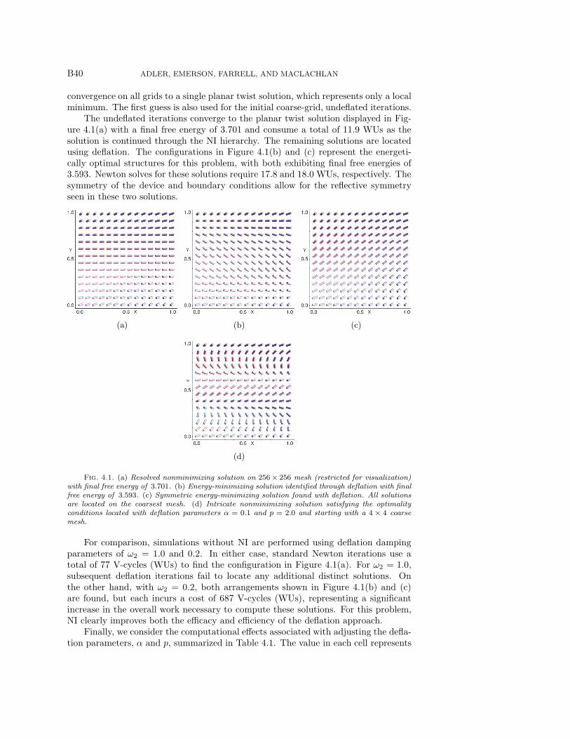
The undeflated iterations converge to the planar twist solution displayed in Fig-ure 4.1(a) with a final free energy of 3.701 and consume a total of 11.9 WUs as thesolution is continued through the NI hierarchy. The remaining solutions are locatedusing deflation. The configurations in Figure 4.1(b) and (c) represent the energeti-cally optimal structures for this problem, with both exhibiting final free energies of3.593. Newton solves for these solutions require 17.8 and 18.0 WUs, respectively. Thesymmetry of the device and boundary conditions allow for the reflective symmetryseen in these two solutions.

(a) (b) (c)

(d)

Fig. 4.1. (a) Resolved nonminimizing solution on 256× 256 mesh (restricted for visualization)with final free energy of 3.701. (b) Energy-minimizing solution identified through deflation with finalfree energy of 3.593. (c) Symmetric energy-minimizing solution found with deflation. All solutionsare located on the coarsest mesh. (d) Intricate nonminimizing solution satisfying the optimalityconditions located with deflation parameters α = 0.1 and p = 2.0 and starting with a 4 × 4 coarsemesh.

For comparison, simulations without NI are performed using deflation dampingparameters of ω2 = 1.0 and 0.2. In either case, standard Newton iterations use atotal of 77 V-cycles (WUs) to find the configuration in Figure 4.1(a). For ω2 = 1.0,subsequent deflation iterations fail to locate any additional distinct solutions. Onthe other hand, with ω2 = 0.2, both arrangements shown in Figure 4.1(b) and (c)are found, but each incurs a cost of 687 V-cycles (WUs), representing a significantincrease in the overall work necessary to compute these solutions. For this problem,NI clearly improves both the efficacy and efficiency of the deflation approach.

Finally, we consider the computational effects associated with adjusting the defla-tion parameters, α and p, summarized in Table 4.1. The value in each cell represents

DEFLATION AND NESTED ITERATION B41

the total number of WUs required in computing all discovered solutions. Each combi-nation of parameters yields the three solutions shown in Figure 4.1(a)–(c), providingexperimental evidence for the robustness of the deflation approach with respect toparameter choice. However, the applied parameters do have a noticeable effect onthe WU efficiency. These fluctuations correspond to changes in the mesh level of theNI hierarchy at which deflation successfully locates additional solutions. For exam-ple, the accrued WUs for α = 0.1 and p = 1.0 are considerably higher than those ofα = 1.0 and p = 3.0 because the third liquid crystal configuration is discovered onthe fourth mesh rather than the coarsest one.

Table 4.1

Total WUs accumulated within the NI hierarchy during the computation of the three configu-rations shown in Figure 4.1(a)–(c) for varying deflation parameters. Note that these WUs do notinclude overhead associated with deflation iterations that did not converge on each grid.

α \ p 1.0 2.0 3.0 4.00.1 82.6 50.8 47.7 47.90.5 65.5 49.3 66.0 66.01.0 64.9 65.8 47.8 57.02.0 65.5 56.9 66.0 57.4

In other experiments, certain setups and selections of deflation parameters mayyield additional distinct solutions. For example, the configuration displayed in Figure4.1(d) is discovered when applying deflation parameters of α = 0.1 and p = 2.0with an NI hierarchy starting on a 4 × 4 coarse mesh. The structure’s free energyis 32.336. While the configuration is clearly not energetically optimal, it satisfiesthe first-order optimality conditions. Further, in section 5.2, the discovery of anadditional, distinct solution with the application of alternative deflation parameterswithout changing the NI hierarchy is briefly discussed. At present, deflation parameterchoice generally relies on numerical experience and experimentation, but current workis focused on constructing a better theoretical understanding of these parameters’effects on convergence and constructing techniques for automatic selection of thesevalues.

4.2. Freedericksz transition. The second numerical experiment considers aclassical Freedericksz transition problem with simple director boundary conditionssuch that n lies uniformly parallel to the x-axis at the edges y = 0 and y = 1. For theelectric potential, φ, the boundary conditions set φ(x, 0) = 0 and φ(x, 1) = V = 1.1.The relevant Frank and electric constants are K1 = 1, K2 = 0.62903, and K3 =1.32258 (those of 5CB), ε0 = 1.42809, ε⊥ = 7, and εa = 11.5. Note that for εa > 0 theliquid crystals are attracted to alignment parallel to the electric field. The relevantdamping parameters are ω1 = 1.0, Δ1 = 0.0, ω2 = 1.0, and Δ2 = 0.5. The sametwo initial guesses for n used in the previous experiment are applied in the deflationsolves here; cf. Appendix B. These configurations serve as the starting point for alldeflation searches in the NI hierarchy.

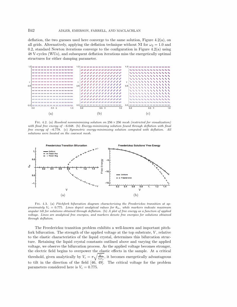
The initial undeflated iterations converge to the elastic rest configuration uni-formly parallel to the x-axis shown in Figure 4.2(a) and use 16.0 WUs. The finalfree energy for this structure is −6.048. Thereafter, using deflation, the energeticallyoptimal arrangements displayed in Figures 4.2(b) and (c) are found, and both havefinal free energies of −6.778. The computation of each solution requires 33.4 WUs.These solutions represent a true Freedericksz transition in which the applied electricfield successfully deforms the nematic configuration away from elastic rest. Without

B42 ADLER, EMERSON, FARRELL, AND MACLACHLAN

deflation, the two guesses used here converge to the same solution, Figure 4.2(a), onall grids. Alternatively, applying the deflation technique without NI for ω2 = 1.0 and0.2, standard Newton iterations converge to the configuration in Figure 4.2(a) using48 V-cycles (WUs), and subsequent deflation iterations miss the energetically optimalstructures for either damping parameter.

(a) (b) (c)

Fig. 4.2. (a) Resolved nonminimizing solution on 256× 256 mesh (restricted for visualization)with final free energy of −6.048. (b) Energy-minimizing solution found through deflation with finalfree energy of −6.778. (c) Symmetric energy-minimizing solution computed with deflation. Allsolutions were located on the coarsest mesh.

(a) (b)

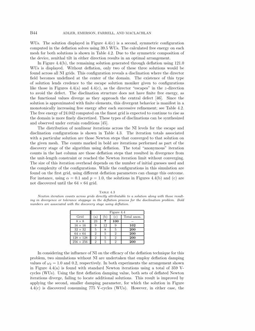
Fig. 4.3. (a) Pitchfork bifurcation diagram characterizing the Freedericksz transition at ap-proximately Vc = 0.775. Lines depict analytical values for θm, while markers indicate maximumangular tilt for solutions obtained through deflation. (b) A plot of free energy as a function of appliedvoltage. Lines are analytical free energies, and markers denote free energies for solutions obtainedthrough deflation.

The Freedericksz transition problem exhibits a well-known and important pitch-fork bifurcation. The strength of the applied voltage at the top substrate, V , relativeto the elastic characteristics of the liquid crystal, determines this bifurcation struc-ture. Retaining the liquid crystal constants outlined above and varying the appliedvoltage, we observe the bifurcation process. As the applied voltage becomes stronger,the electric field begins to overpower the elastic effects in the sample. At a critical

threshold, given analytically by Vc = π√

K1

ε0εa, it becomes energetically advantageous

to tilt in the direction of the field [46, 49]. The critical voltage for the problemparameters considered here is Vc = 0.775.

DEFLATION AND NESTED ITERATION B43

In Figure 4.3(a), when V reaches the critical value, solutions tilting in the directionof the electric field begin to satisfy the first-order optimality conditions and yieldoptimal free energy. The value θm denotes the maximum angular tilt of the directorfield in the direction of the electric field resulting from the applied voltage. Figure4.3(b) characterizes the shift in free-energy optimizing solutions resulting from theFreedericksz transition as V passes the critical voltage, Vc. In both figures, the linesrepresent analytical computations as V varies [46], and the individual markers arevalues for solutions computed independently for each value of V through deflation.

4.3. Escape and disclination solutions. This third numerical experiment in-vestigates the phenomenon of defects, also known as disclinations. Defects in liquidcrystal structures are locations in a sample where the director field is undefined orcontains discontinuities. There are a multitude of disclination types, including point,wedge, sheet, and loop defects. In this example, we consider wedge disclinations.These disclinations involve rotation around an axis parallel to the defect and aretherefore sometimes referred to as axial disclinations [25]. Wedge-type disclinationshave been studied in [19, 23].

For this simulation, the damping parameters are ω1 = 0.4, Δ1 = 0.2, ω2 =1.0, and Δ2 = 0.5. Dirichlet boundary conditions are applied to the entire domainboundary, and no electric field is present. The boundary conditions are fixed suchthat the director faces the center of the domain and Frank constants of K1 = 1.0,K2 = 3.0, and K3 = 1.2 are used. As in the previous experiments, two initial guesses,detailed in Appendix B, are used for the deflation solves on each grid.

(a) (b) (c)

Fig. 4.4. (a) Resolved escape solution on 256 × 256 mesh (restricted for visualization) withfinal free energy of 9.971. (b) Disclination solution with central wedge defect and final free energyof 24.042 (free energy is expected to diverge with refinement). (c) Symmetric escape solution withfinal free energy of 9.971.

Table 4.2

Computed free energies on each mesh for the set of computed solutions.

Grid 8× 8 16× 16 32× 32 64× 64 128× 128 256 × 256

Pos. escape 9.972 9.971 9.971 9.971 9.971 9.971Disclination 13.154 15.331 17.509 19.686 21.864 24.042Neg. escape 9.971 9.971 9.971 9.971 9.971 9.971

The first solution, located using undeflated solves, is displayed in Figure 4.4(a).This director field is continuous and shares some similarities with the solutions foundin [11, 39] for long cylindrical capillaries. The progression of the solves consumes 38.4

B44 ADLER, EMERSON, FARRELL, AND MACLACHLAN

WUs. The solution displayed in Figure 4.4(c) is a second, symmetric configurationcomputed in the deflation solves using 39.5 WUs. The calculated free energy on eachmesh for both solutions is shown in Table 4.2. Due to the symmetric composition ofthe device, zenithal tilt in either direction results in an optimal arrangement.

In Figure 4.4(b), the remaining solution generated through deflation using 121.0WUs is displayed. Without deflation, only two of these three solutions would befound across all NI grids. This configuration reveals a disclination where the directorfield becomes undefined at the center of the domain. The existence of this typeof solution lends credence to the escape solution moniker given to configurationslike those in Figures 4.4(a) and 4.4(c), as the director “escapes” in the z-directionto avoid the defect. The disclination structure does not have finite free energy, asthe functional values diverge as they approach the central defect [46]. Since thesolution is approximated with finite elements, this divergent behavior is manifest in amonotonically increasing free energy after each successive refinement; see Table 4.2.The free energy of 24.042 computed on the finest grid is expected to continue to rise asthe domain is more finely discretized. These types of disclinations can be synthesizedand observed under certain conditions [45].

The distribution of nonlinear iterations across the NI levels for the escape anddisclination configurations is shown in Table 4.3. The iteration totals associatedwith a particular solution are those Newton steps that converged to that solution onthe given mesh. The counts marked in bold are iterations performed as part of thediscovery stage of the algorithm using deflation. The total “anonymous” iterationcounts in the last column are those deflation steps that resulted in divergence fromthe unit-length constraint or reached the Newton iteration limit without converging.The size of this iteration overhead depends on the number of initial guesses used andthe complexity of the configurations. While the configurations in this simulation arefound on the first grid, using different deflation parameters can change this outcome.For instance, using α = 0.1 and p = 1.0, the solutions in Figures 4.4(b) and (c) arenot discovered until the 64× 64 grid.

Table 4.3

Newton iteration counts across grids directly attributable to a solution along with those result-ing in divergence or tolerance stoppage in the deflation process for the disclination problem. Boldnumbers are associated with the discovery stage using deflation.

Figure 4.4

Grid (a) (b) (c) Total anon.

8× 8 23 7 100 −16× 16 9 12 9 10232× 32 5 8 5 20064× 64 2 5 2 200

128 × 128 2 5 2 200256 × 256 2 5 2 200

In considering the influence of NI on the efficacy of the deflation technique for thisproblem, two simulations without NI are undertaken that employ deflation dampingvalues of ω2 = 1.0 and 0.2, respectively. In both experiments the arrangement shownin Figure 4.4(a) is found with standard Newton iterations using a total of 359 V-cycles (WUs). Using the first deflation damping value, both sets of deflated Newtoniterations diverge, failing to locate additional solutions. This result is improved byapplying the second, smaller damping parameter, for which the solution in Figure4.4(c) is discovered consuming 775 V-cycles (WUs). However, in either case, the

DEFLATION AND NESTED ITERATION B45

disclination solution remains undiscovered. A possible cause for missing this solutionis the fact that the coarse-grid representations of the escape and disclination solutionsare energetically closer to one another compared with those of finer-scale meshes,as seen in Table 4.2. As the disclination configuration’s free energy diverges, thelikelihood of deflated iterations reaching its basin of attraction may shrink.

Table 4.4

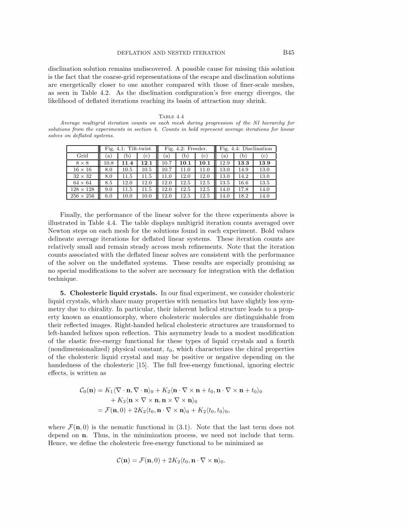
Average multigrid iteration counts on each mesh during progression of the NI hierarchy forsolutions from the experiments in section 4. Counts in bold represent average iterations for linearsolves on deflated systems.

Fig. 4.1: Tilt-twist Fig. 4.2: Freeder. Fig. 4.4: Disclination

Grid (a) (b) (c) (a) (b) (c) (a) (b) (c)

8× 8 10.8 11.4 12.1 10.7 10.1 10.1 12.9 13.3 13.916× 16 8.0 10.5 10.5 10.7 11.0 11.0 13.0 14.9 13.032× 32 8.0 11.5 11.5 11.0 12.0 12.0 13.0 14.2 13.064× 64 8.5 12.0 12.0 12.0 12.5 12.5 13.5 16.6 13.5

128× 128 9.0 11.5 11.5 12.0 12.5 12.5 14.0 17.8 14.0256× 256 6.0 10.0 10.0 12.0 12.5 12.5 14.0 18.2 14.0

Finally, the performance of the linear solver for the three experiments above isillustrated in Table 4.4. The table displays multigrid iteration counts averaged overNewton steps on each mesh for the solutions found in each experiment. Bold valuesdelineate average iterations for deflated linear systems. These iteration counts arerelatively small and remain steady across mesh refinements. Note that the iterationcounts associated with the deflated linear solves are consistent with the performanceof the solver on the undeflated systems. These results are especially promising asno special modifications to the solver are necessary for integration with the deflationtechnique.

5. Cholesteric liquid crystals. In our final experiment, we consider cholestericliquid crystals, which share many properties with nematics but have slightly less sym-metry due to chirality. In particular, their inherent helical structure leads to a prop-erty known as enantiomorphy, where cholesteric molecules are distinguishable fromtheir reflected images. Right-handed helical cholesteric structures are transformed toleft-handed helixes upon reflection. This asymmetry leads to a modest modificationof the elastic free-energy functional for these types of liquid crystals and a fourth(nondimensionalized) physical constant, t0, which characterizes the chiral propertiesof the cholesteric liquid crystal and may be positive or negative depending on thehandedness of the cholesteric [15]. The full free-energy functional, ignoring electriceffects, is written as

C0(n) = K1〈∇ · n,∇ · n〉0 +K2〈n · ∇ × n+ t0,n · ∇ × n+ t0〉0+K3〈n×∇× n,n×∇× n〉0

= F(n, 0) + 2K2〈t0,n · ∇ × n〉0 +K2〈t0, t0〉0,

where F(n, 0) is the nematic functional in (3.1). Note that the last term does notdepend on n. Thus, in the minimization process, we need not include that term.Hence, we define the cholesteric free-energy functional to be minimized as

C(n) = F(n, 0) + 2K2〈t0,n · ∇ × n〉0.

B46 ADLER, EMERSON, FARRELL, AND MACLACHLAN

5.1. Minimization. Since cholesterics are subject to the same pointwise unit-length constraint as nematics, the Lagrangian is formed as

LC(n, λ) = C(n) +∫Ω

λ(n · n− 1) dV.

Computing the derivative of LC with respect to n yields

LCn (n, λ)[w] = Ln[w] + 2K2 (〈t0,w · ∇ × n〉0 + 〈t0,n · ∇ ×w〉0) .

Because the additional terms of the free energy specific to cholesterics do not dependon λ, derivatives of this Lagrangian involving λ are identical to those of the nematiccase. Thus, in computing the Hessian, the only derivative with additional terms isthe second-order derivative with respect to n, giving

LCnn = Lnn + 2K2 (〈t0,w · ∇ × δn〉0 + 〈t0, δn · ∇ ×w〉0) .

Modifying the energy-minimization and deflation algorithm discussed above for ne-matics by adding in the appropriate terms corresponding to the cholesteric free en-ergy yields an effective algorithm for computing multiple equilibrium configurationsof cholesteric liquid crystals.

5.2. Chiral configuration. In this simulation, we consider a simple cholestericconfiguration, using the same mixed periodic and Dirichlet boundary conditions andslab domain assumption as in previous numerical examples. At the Dirichlet bound-ary, uniform conditions such that n = (1, 0, 0) are enforced. In the case of nematicliquid crystals, subject to elastic forces, the minimizing configuration is full align-ment parallel to the director on the boundary. However, the energetically optimalarrangement for cholesterics is a chiral configuration along the y-axis with twist prop-erties determined by the value of t0. Using an ansatz for a chiral solution of the formn = (cos(τy), 0,− sin(τy)), the computations in [46] can be modified to our coordinatesystem, giving the elastic free energy associated with this ansatz as 1

2K2(t0 − τ)2|Ω|,where |Ω| is the domain measure, so long as the chiral ansatz also conforms tothe imposed boundary conditions. Since the elastic free energy is positive andsemidefinite, clearly the free energy of the ansatz is minimized when τ = t0; whent0 is an integer multiple of 2π, the uniform Dirichlet boundary conditions above willalso be satisfied.

For this numerical simulation, the Frank constants are set to K1 = 1.0, K2 = 3.0,and K3 = 1.2, while t0 = −2π. This implies that the energy-minimizing solutioncorresponds to a left-handed helix running parallel to the y-axis with a 2π-rotationacross the device. However, additional configurations, while not globally minimizing,satisfy the first-order optimality conditions and are experimentally observable.

The deflation algorithm is applied with damping values of ω1 = 0.2, Δ1 = 0.2,ω2 = 0.2, and Δ2 = 0.0. Using the set of three initial guesses outlined in AppendixB, the algorithm reveals a rich set of solutions satisfying the optimality conditions.A total of six distinct solutions, shown in Figure 5.1, are found, whereas, withoutdeflation, only three solutions would be identified across all grids. The correspondingcomputed free energies for these solutions are shown in Table 5.1 along with averageiteration counts for the multigrid-preconditioned GMRES linear solver. In general, thelinear solver iteration counts are higher for these cholesteric systems compared withthose of the previous section. Correspondingly, the WUs, shown in the same table,are larger when compared with previous experiments. This increase in iterations is

DEFLATION AND NESTED ITERATION B47

(a) (b) (c)

(d) (e) (f)

Fig. 5.1. Family of distinct solutions for the cholesteric equilibrium problem found throughdeflation. Each solution is computed on a 256 × 256 mesh and restricted for visualization. Theenergy minimizing solution is displayed in (c).

most likely due to a combination of the additional term in the cholesteric functionaland higher overall free energies in the solutions. However, the iterations counts arerelatively consistent across grid refinements, and the average solver iterations for thedeflated systems, shown in bold, correspond well with the iteration counts for theundeflated solves.

Table 5.1

Average multigrid iteration counts on each mesh during progression of the NI hierarchy forthe cholesteric experiment above. Counts in bold represent average iterations for linear solves ondeflated systems. The final rows display the WUs and free energy associated with each computedequilibrium configuration.

Figure 5.1

Grid (a) (b) (c) (d) (e) (f)

8× 8 46.2 52.9 11.3 − − −16 × 16 66.0 54.3 9.0 67.7 66.8 −32 × 32 65.0 33.2 8.0 53.9 34.1 −64 × 64 61.0 28.4 8.0 35.8 26.9 −

128 × 128 62.0 33.0 9.0 52.5 32.5 29.0256 × 256 78.0 30.5 9.5 46.0 30.0 18.5

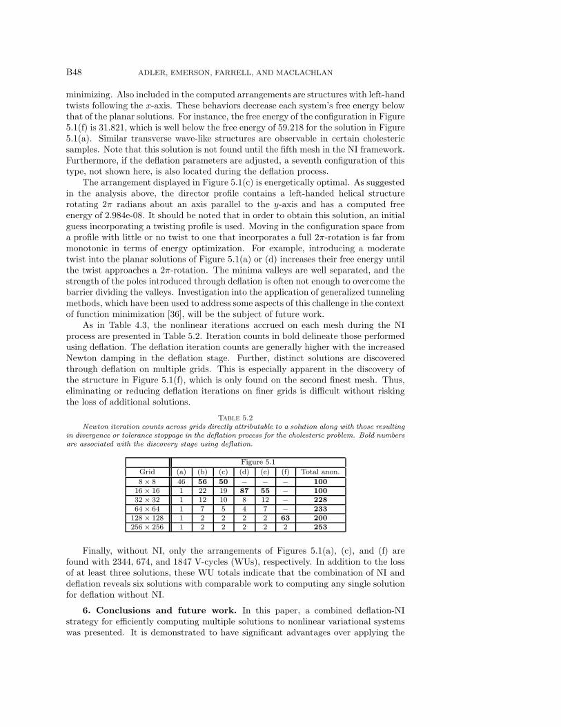
Work units 100.7 103.7 28.5 156.9 108.7 493.0Free energy 59.218 56.553 2.984e-08 59.378 56.553 31.821

The solution set includes degenerate planar solutions displayed in Figures 5.1(a)and (d). By virtue of the chirality of cholesterics, these configurations are not globally

B48 ADLER, EMERSON, FARRELL, AND MACLACHLAN

minimizing. Also included in the computed arrangements are structures with left-handtwists following the x-axis. These behaviors decrease each system’s free energy belowthat of the planar solutions. For instance, the free energy of the configuration in Figure5.1(f) is 31.821, which is well below the free energy of 59.218 for the solution in Figure5.1(a). Similar transverse wave-like structures are observable in certain cholestericsamples. Note that this solution is not found until the fifth mesh in the NI framework.Furthermore, if the deflation parameters are adjusted, a seventh configuration of thistype, not shown here, is also located during the deflation process.

The arrangement displayed in Figure 5.1(c) is energetically optimal. As suggestedin the analysis above, the director profile contains a left-handed helical structurerotating 2π radians about an axis parallel to the y-axis and has a computed freeenergy of 2.984e-08. It should be noted that in order to obtain this solution, an initialguess incorporating a twisting profile is used. Moving in the configuration space froma profile with little or no twist to one that incorporates a full 2π-rotation is far frommonotonic in terms of energy optimization. For example, introducing a moderatetwist into the planar solutions of Figure 5.1(a) or (d) increases their free energy untilthe twist approaches a 2π-rotation. The minima valleys are well separated, and thestrength of the poles introduced through deflation is often not enough to overcome thebarrier dividing the valleys. Investigation into the application of generalized tunnelingmethods, which have been used to address some aspects of this challenge in the contextof function minimization [36], will be the subject of future work.

As in Table 4.3, the nonlinear iterations accrued on each mesh during the NIprocess are presented in Table 5.2. Iteration counts in bold delineate those performedusing deflation. The deflation iteration counts are generally higher with the increasedNewton damping in the deflation stage. Further, distinct solutions are discoveredthrough deflation on multiple grids. This is especially apparent in the discovery ofthe structure in Figure 5.1(f), which is only found on the second finest mesh. Thus,eliminating or reducing deflation iterations on finer grids is difficult without riskingthe loss of additional solutions.

Table 5.2

Newton iteration counts across grids directly attributable to a solution along with those resultingin divergence or tolerance stoppage in the deflation process for the cholesteric problem. Bold numbersare associated with the discovery stage using deflation.

Figure 5.1

Grid (a) (b) (c) (d) (e) (f) Total anon.

8× 8 46 56 50 − − − 10016 × 16 1 22 19 87 55 − 10032 × 32 1 12 10 8 12 − 22864 × 64 1 7 5 4 7 − 233

128 × 128 1 2 2 2 2 63 200256 × 256 1 2 2 2 2 2 253

Finally, without NI, only the arrangements of Figures 5.1(a), (c), and (f) arefound with 2344, 674, and 1847 V-cycles (WUs), respectively. In addition to the lossof at least three solutions, these WU totals indicate that the combination of NI anddeflation reveals six solutions with comparable work to computing any single solutionfor deflation without NI.

6. Conclusions and future work. In this paper, a combined deflation-NIstrategy for efficiently computing multiple solutions to nonlinear variational systemswas presented. It is demonstrated to have significant advantages over applying the

DEFLATION AND NESTED ITERATION B49

existing deflation methodology on a single grid. In particular, the combined approachretains the efficiency expected of NI algorithms for nonlinear PDEs while enhancingthe deflation approach’s ability to expose multiple solutions. As with the originaldeflation methodology, we are able to reuse existing linear solvers for linearizations ofthe undeflated system, further enhancing the computational efficiency of the combinedapproach.

Four numerical simulations were conducted with the combined algorithm, demon-strating the effectiveness of this approach for problems in the numerical simulationof nematic and cholesteric liquid crystals. In all cases, multiple solutions are found,including global minima, and correct bifurcation structures are computed for the free-energy model in two cases where these are known analytically. The effectiveness ofthe algorithm considered here is expected to inform the application of the deflationmethod for a more general class of constrained optimization and multiphysics prob-lems, including closely related models in ferromagnetics. Future work will considerconstruction of a generalized tunneling approach, based on the work in [36], appliedto the Newton iterations to further increase the power of the deflation method. Inaddition, we aim to investigate the method’s performance in analyzing new physicalphenomena and behaviors in shaped domains. Finally, strategies for adaptive con-struction of initial guesses for the deflation method at each level of the NI process willbe studied.

Appendix A. Hessian of the nematic model. In this appendix, we detailthe full expressions for each component of the Hessian in (3.5). The multiplicativenotation indicates the direction associated with each derivative. For instance, Lλn[γ] ·δn = ∂

∂n (Lλ(nk, φk, λk)[γ]) [δn], where the partials indicate Gateaux derivatives inthe respective variables. Thus, each term of the Hessian is written as

Lnn[w] · δn = 2K1〈∇ · δn,∇ ·w〉0 + 2K3〈Z(nk)∇× δn,∇×w〉0+ 2(K2 −K3)

(〈δn · ∇ ×w,nk · ∇ × nk〉0

+ 〈nk · ∇ ×w, δn · ∇ × nk〉0 + 〈nk · ∇ × nk,w · ∇ × δn〉0+ 〈nk · ∇ × δn,w · ∇ × nk〉0 + 〈δn · ∇ × nk,w · ∇ × nk〉0

)− 2ε0εa〈δn · ∇φk,w · ∇φk〉0 + 2

∫Ω

λk(δn,w) dV,

Lnφ[w] · δφ = −2ε0εa〈nk · ∇φk,w · ∇δφ〉0 − 2ε0εa〈nk · ∇δφ,w · ∇φk〉0,Lnλ[w] · δλ = 2

∫Ω

δλ(nk,w) dV,

Lφn[ψ] · δn = −2ε0εa〈nk · ∇φk, δn · ∇ψ〉0 − 2ε0εa〈δn · ∇φk,nk · ∇ψ〉0,Lφφ[ψ] · δφ = −2ε0ε⊥〈∇δφ,∇ψ〉0 − 2ε0εa〈nk · ∇δφ,nk · ∇ψ〉0,Lλn[γ] · δn = 2

∫Ω

γ(nk, δn) dV.

Additional details are found in [1].

Appendix B. Initial guesses. In this appendix, we report the initial guessesused for each example to aid in reproducing the results. Each guess listed here givesthe values used on the interior of the domain for all NI levels; the Dirichlet bound-ary conditions are enforced along the relevant boundaries. In all of the simulationsperformed, λ is initially set to 0.

B50 ADLER, EMERSON, FARRELL, AND MACLACHLAN

In sections 4.1 and 4.2, the initial guesses used were n = (cos( π40 ), sin(

π40 ), 0) and

n = (cos( π40 ),− sin( π

40 ), 0). In addition, the simulations of section 4.2 use φ = V · y toinitialize the electric potential for both guesses, where V is the potential at the topsubstrate.

For section 4.3, let ξ1 = | tan−1( 0.5−y0.5−x )|, ζ1 = 9π

20 , and define the functions

n1 =

{sin(ζ1) cos(ξ1) if x ≤ 0.5,

− sin(ζ1) cos(ξ1) if x > 0.5,n2 =

{sin(ζ1) sin(ξ1) if y ≤ 0.5,

− sin(ζ1) sin(ξ1) if y > 0.5,

n3 = cos(ζ1).

Then the two initial values for the director in the section are given by

n =

{(0, 0, 1

)if x, y = 0.5,(

n1, n2, n3

)otherwise,

n =

{(0, 0, 1

)if x, y = 0.5,(

n1, n2,−n3

)otherwise.

Finally, for section 5.2, let ξ2 = 7π16 and ζ2 = π

4 . The initial values for n are shownin Table B.1.

Table B.1

Formulas for the initial guesses used in section 5.2.

Guess 1 Guess 2 Guess 3

n1 = cos (π/12)

n2 = sin (π/12)

n3 = 0

n1 = sin (ξ2) cos(ζ2 cos(4πx)

)

n2 = sin (ξ2) sin(ζ2 cos(4πx)

)

n3 = cos(ξ2)

n1 = cos (2πy) cos (π/8)

n2 = cos (2πy) sin (π/8)

n3 = sin(2πy)

Acknowledgments. The authors would like to thank Professor Timothy Ather-ton for his useful suggestions and guidance and Dr. Thomas Benson for allowing us toadapt his code. We would also like to thank the anonymous referees for their helpfulcomments that improved the quality of this paper.

REFERENCES

[1] J. H. Adler, T. J. Atherton, T. R. Benson, D. B. Emerson, and S. P. MacLachlan,Energy minimization for liquid crystal equilibrium with electric and flexoelectric effects,SIAM J. Sci. Comput., 37 (2015), pp. S157–S176, https://doi.org/10.1137/140975036.

[2] J. H. Adler, T. J. Atherton, D. B. Emerson, and S. P. MacLachlan, An energy-minimization finite-element approach for the Frank–Oseen model of nematic liquid crys-tals, SIAM J. Numer. Anal., 53 (2015), pp. 2226–2254, https://doi.org/10.1137/140956567.

[3] J. H. Adler, T. R. Benson, E. C. Cyr, S. P. MacLachlan, and R. S. Tuminaro, Mono-lithic multigrid methods for two-dimensional resistive magnetohydrodynamics, SIAM J.Sci. Comput., 38 (2016), pp. B1–B24, https://doi.org/10.1137/151006135.

[4] J. H. Adler, J. Brannick, C. Liu, T. Manteuffel, and L. Zikatanov, First-order systemleast squares and the energetic variational approach for two-phase flow, J. Comput. Phys.,230 (2011), pp. 6647–6663.

[5] J. H. Adler, D. B. Emerson, S. P. MacLachlan, and T. A. Manteuffel, Constrainedoptimization for liquid crystal equilibria, SIAM J. Sci. Comput., 38 (2016), pp. B50–B76,https://doi.org/10.1137/141001846.

[6] J. H. Adler, T. A. Manteuffel, S. F. McCormick, J. W. Ruge, and G. D. Sanders,Nested iteration and first-order system least squares for incompressible, resistive magne-tohydrodynamics, SIAM J. Sci. Comput., 32 (2010), pp. 1506–1526, https://doi.org/10.1137/090766905.

[7] T. J. Atherton and J. H. Adler, Competition of elasticity and flexoelectricity for bistablealignment of nematic liquid crystals on patterned surfaces, Phys. Rev. E, 86 (2012), 040701,https://doi.org/10.1103/PhysRevE.86.040701.

DEFLATION AND NESTED ITERATION B51

[8] T. J. Atherton and J. R. Sambles, Orientational transition in a nematic liquid crystal ata patterned surface, Phys. Rev. E, 74 (2006), 022701, https://doi.org/10.1103/PhysRevE.74.022701.

[9] W. Bangerth, R. Hartmann, and G. Kanschat, deal.II—a general-purpose object-orientedfinite element library, ACM Trans. Math. Software, 33 (2007), 24.

[10] R. H. Byrd, R. B. Schnabel, and G. A. Shultz, A trust region algorithm for nonlinearlyconstrained optimization, SIAM J. Numer. Anal., 24 (1987), pp. 1152–1170, https://doi.org/10.1137/0724076.

[11] P. E. Cladis and M. Kleman, Non-singular disclinations of strength S = +1 in nematics, J.de Physique, 33 (1972), pp. 591–598.

[12] A. L. Codd, T. A. Manteuffel, and S. F. McCormick, Multilevel first-order system leastsquares for nonlinear elliptic partial differential equations, SIAM J. Numer. Anal., 41(2003), pp. 2197–2209, https://doi.org/10.1137/S0036142902404406.

[13] R. Cohen, R. Hardt, D. Kinderlehrer, S. Lin, and M. Luskin, Minimum energy config-urations for liquid crystals: Computational results, in Theory and Applications of LiquidCrystals, IMA Vol. Math. Appl. 5, Springer-Verlag, New York, 1987, pp. 99–121.

[14] P. J. Collings, Liquid Crystals: Nature’s Delicate Phase of Matter, Adam Hilger, Bristol,UK, 1990.

[15] P. J. Collings and M. Hird, Introduction to Liquid Crystals, Taylor and Francis, London,1997.

[16] T. A. Davis and E. C. Gartland, Jr., Finite element analysis of the Landau–de Gennesminimization problem for liquid crystals, SIAM J. Numer. Anal., 35 (1998), pp. 336–362,https://doi.org/10.1137/S0036142996297448.

[17] P. G. de Gennes and J. Prost, The Physics of Liquid Crystals, 2nd ed., Clarendon Press,Oxford, UK, 1993.

[18] H. J. Deuling, Deformation of nematic liquid crystals in an electric field, Mol. Cryst. Liq.Cryst., 19 (1972), pp. 123–131.

[19] I. E. Dzylaoshinskii, Theory of disclinations in liquid crystals, Sov. Phys. JETP, 31 (1970),pp. 773–777.

[20] J. L. Ericksen, Hydrostatic theory of liquid crystals, Arch. Ration. Mech. Anal., 9 (1962),pp. 371–378.

[21] J. L. Ericksen, Inequalities in liquid crystal theory, Phys. Fluids, 9 (1966), pp. 1205–1207.

[22] P. E. Farrell, A. Birkisson, and S. W. Funke, Deflation techniques for finding distinctsolutions of nonlinear partial differential equations, SIAM J. Sci. Comput., 37 (2015),pp. A2026–A2045, https://doi.org/10.1137/140984798.

[23] F. C. Frank, On the theory of liquid crystals, Discuss. Faraday Soc., 25 (1958), pp. 19–28.[24] V. Freedericksz and V. Zolina, Forces causing the orientation of an anisotropic liquid,

Trans. Faraday Soc., 29 (1933), pp. 919–930.[25] J. Friedel and P. G. de Gennes, Boucles de disclination dans les cristaux liquides, C. R.

Acad. Sc. Paris B, 268 (1969), pp. 257–259.[26] E. C. Gartland, Jr., and A. Ramage, A renormalized Newton method for liquid crystal

director modeling, SIAM J. Numer. Anal., 53 (2015), pp. 251–278, https://doi.org/10.1137/130942917.

[27] L. Gattermann and A. Ritschke, Uber azoxyphenolather, Ber. Deutsche. Chem. Ges., 23(1890), pp. 1738–1750.

[28] V. Girault and P. Raviart, Finite Element Methods for Navier-Stokes Equations: Theoryand Algorithms, Springer-Verlag, Berlin, 1986.

[29] M. D. Gunzburger, A. J. Meir, and J. S. Peterson, On the existence, uniqueness, andfinite element approximation of solutions of the equations of stationary, incompressiblemagnetohydrodynamics, Math. Comp., 56 (1991), pp. 523–563.

[30] W. W. Hager, Updating the inverse of a matrix, SIAM Rev., 31 (1989), pp. 221–239, https://doi.org/10.1137/1031049.

[31] Q. Hu, X.-C. Tai, and R. Winther, A saddle point approach to the computation of har-monic maps, SIAM J. Numer. Anal., 47 (2009), pp. 1500–1523, https://doi.org/10.1137/060675575.

[32] M. Kruzık and A. Prohl, Recent developments in the modeling, analysis, and numer-ics of ferromagnetism, SIAM Rev., 48 (2006), pp. 439–483, https://doi.org/10.1137/S0036144504446187.

[33] J. P. F. Lagerwall and G. Scalia, A new era for liquid crystal research: Applications ofliquid crystals in soft matter, nano-, bio- and microtechnology, Curr. Appl. Phys., 12(2012), pp. 1387–1412.

B52 ADLER, EMERSON, FARRELL, AND MACLACHLAN

[34] B. W. Lee and N. A. Clark, Alignment of liquid crystals with patterned isotropic surfaces,Science, 291 (2001), pp. 2576–2580.

[35] F. M. Leslie, Distorted twisted orientation patterns in nematic liquid crystals, Pramana,Suppl. No., 1 (1975), pp. 41–55.

[36] A. V. Levy and S. Gomez, The tunneling method applied to global optimization, in NumericalOptimization, P. T. Boggs, R. H. Byrd, and R. B. Schnabel, eds., SIAM, Philadelphia,1985, pp. 213–244.

[37] T. A. Manteuffel, S. F. McCormick, J. G. Schmidt, and C. R. Westphal, First-ordersystem least squares for geometrically nonlinear elasticity, SIAM J. Numer. Anal., 44(2006), pp. 2057–2081, https://doi.org/10.1137/050628027.

[38] R. Martı, Multi-start methods, in Handbook in Metaheuristics, International Series in Op-erations Research & Management Science 57, F. Glover and G. A. Kochenberger, eds.,Springer, New York, 2003, pp. 355–368.

[39] R. B. Meyer, On the existence of even indexed disclinations in nematic liquid crystals, Phil.Mag., 27 (1973), pp. 405–424.

[40] L. Onsager, The effects of shape on the interaction of colloidal particles, Ann. New YorkAcad. Sci., 51 (1949), pp. 627–659.

[41] A. Pandolfi and G. Napoli, A numerical investigation of configurational distortions in ne-matic liquid crystals, J. Nonlinear Sci., 21 (2011), pp. 785–809.

[42] A. Ramage and E. C. Gartland, Jr., A preconditioned nullspace method for liquid crystaldirector modeling, SIAM J. Sci. Comput., 35 (2013), pp. B226–B247, https://doi.org/10.1137/120870219.

[43] R. R. Shah and N. L. Abbott, Principles for measurement of chemical exposure based onrecognition-driven anchoring transitions in liquid crystals, Science, 293 (2001), pp. 1296–1299.

[44] G. Starke, Gauss-Newton multilevel methods for least-squares finite element computations ofvariably saturated subsurface flow, Computing, 64 (2000), pp. 323–338.

[45] M. J. Stephen and J. P. Straley, Physics of liquid crystals, Rev. Modern Phys., 46 (1974),pp. 617–704.

[46] I. W. Stewart, The Static and Dynamic Continuum Theory of Liquid Crystals: A Mathe-matical Introduction, Taylor and Francis, London, 2004.

[47] E. G. Virga, Variational Theories for Liquid Crystals, Chapman and Hall, London, 1994.[48] M. Yamada, M. Kondo, J. Mamiya, Y. Yu, M. Kinoshita, C. Barrett, and T. Ikeda,

Photomobile polymer materials: Towards light-driven plastic motors, Angew. Chem. Int.,47 (2008), pp. 4986–4988.

[49] H. Zocher, Uber die Einwirkung magnetischer, elektrischer und mechanischer Krafte aufMesophasen, Physik. Zietschr., 28 (1927), pp. 790–796.