Combinatorial Laplacians of Simplicial Complexes
70
Combinatorial Laplacians of Simplicial Complexes A Senior Project submitted to The Division of Natural Science and Mathematics of Bard College by Timothy E. Goldberg Annandale-on-Hudson, New York May, 2002
Transcript of Combinatorial Laplacians of Simplicial Complexes
Combinatorial Laplacians of Simplicial
Complexes
A Senior Project submitted to
The Division of Natural Science and Mathematics
of
Bard College
by
Timothy E. Goldberg
Annandale-on-Hudson, New York
May, 2002
Abstract
In this paper, we study the combinatorial Laplacian operator on the vector space of ori-ented chains over R of a finite simplicial complex. We develop an easy method of computingthe matrix of this operator from the adjacencies of simplices in the simplicial complex, andthen apply this and results from linear algebra and simplicial homology to study prop-erties of the Laplacian operator and its spectrum. We examine and explore connectionsbetween the combinatorial structure of simplicial complexes and their Laplacian spectra.Specific examples studied include certain classes of graphs and higher dimensional simpli-cial complexes, in particular cones of simplicial complexes, especially simplicial cones ofdimension 2.

Dedication
To my parents, for supporting me on whatever path I take,
and
To Paul, Grandma, Judy, and Grandmom, who probably would not have understood aword of this, but who would have loved it anyway.
Acknowledgments
Let me warn you, I am not known for my brevity.This project would not have been possible without my project advisor, Ethan Bloch,
who provided incalculable expertise, energy, cheerfulness, and boundless enthusiasm, evenwhen I started talking about graph theory. His meticulous and untiring attention to detailand careful craftsmanship, expressed as ominous and indestructible spider webs of red ink,was absolutely invaluable and very nearly painless, and was never expressed without thedeepest kindness. This project would also not have been possible without my other projectadvisor, Lauren Rose, who was the first mathematician I ever worked with at Bard, andwhose passion, experience, knowledge, and skill taught me as much by example as byexplicit instruction. Both of them have my eternal and deepest gratitude.
I owe a great deal to the entire extended mathematics department family, includingEthan and Lauren, but also Mark Halsey, Robert McGrail, Ranny Bledsoe, RebeccaThomas, Sven Anderson, Robert Cutler, and Matthew Deady, who each provided a dif-ferent viewpoint into this wacky world of mathematics, but who have one and all demon-strated to me an inspiring passion for their subjects.
Mark, thank you for showing me that mathematicians are fully capable of being almostpreternaturally serene and calm, unbelievably organized, and still supremely enthusiasticand, well, great. Bob, thank you for showing me some of the most fascinating and beautifulmathematics I have ever seen, which I probably would not have seen but for you.
I also want to thank Professor Victor Reiner from the University of Minnesota andProfessor Robin Forman from Rice University, for being nice enough to meet with us andtalk about Laplacians, and for pointing me in the right direction.
Thank you Professors Christopher Lindner and John Ferguson, for luring me into BardAsylum in the first place.
Thank you David Shein, for being a fantastic boss (even though you always made funof us “math geeks”), for teaching me so much about how to help people, and for always
4
being seriously concerned about the welfare of your slaves, ahem, employees, least of allme.
Thank you April, for your friendship, strength, wisdom, and encouragement, and forshowing me by example that the best creative work requires diligence, patience, and aboveall, passion.
Forget the project – I would not be possible without my parents, Kenneth and JeanneGoldberg. My father taught me a love for all things mathematical, and many things not,and told me bedtime stories about Galois and Willie Mays when I was 7. My mother taughtme how to be passionate about things, and about how to be a functioning, reasoning,and reasonable human being, emotions and all. You both taught me the value of rationalthought balanced by kindness and fun, and you are by far the best role models and raisers-of-children that I can ever imagine existing. And Rebecca, Andrew, and Mean Uncle Bill,thank you for always supporting me in all the work I choose to do, even if you don’t likemath. I’m sorry for every time I tricked you into doing math at the dinner table. (Notreally.)
And of course, I want to thank all of my friends, the ones I knew before Bard, the ones Imet at Bard, and the ones I met last week. Each of you, without exception, is an incrediblywonderful and fine human being, and special and meaningful to me beyond measure, andcertainly beyond my ability to write in only a few words. A brief and certainly incompletelist of people who have my undying gratitude and love is Collin, Valerie, Ethan, Kira,Kisha, Megan, Peter, Vasi, Elena (if I have been able to see further, it was only because Istood on the shoulders of Romanians), Elizabeth, and Jaren.
Thank you everybody. And now, on with the show!
Contents
Abstract 1
Dedication 2
Acknowledgments 3
1 Introduction 8
2 Algebraic Preliminaries 10
2.1 Some Group Theory - Adjoint Homomorphisms . . . . . . . . . . . . . . . . 10
2.2 Some Linear Algebra - Eigenvalues and Eigenvectors . . . . . . . . . . . . . 13
3 Combinatorial Laplacians of Simplicial Complexes 22
3.1 Laplacians in Graph Theory . . . . . . . . . . . . . . . . . . . . . . . . . . . 22
3.2 Simplicial Complexes – Preliminaries . . . . . . . . . . . . . . . . . . . . . . 23
3.3 Laplacians of Simplicial Complexes . . . . . . . . . . . . . . . . . . . . . . . 27
3.4 Reduced Laplacians of Simplicial Complexes . . . . . . . . . . . . . . . . . . 33
4 Laplacian Spectra of Simplicial Complexes 38
4.1 Spectra of ∆, ∆̃, ∆UP , and ∆DN . . . . . . . . . . . . . . . . . . . . . . . . 38
4.2 Further Facts about Laplacian Spectra . . . . . . . . . . . . . . . . . . . . . 43
5 Laplacian Spectra of Specific Complexes 47
5.1 Flapoid Clusters, Cliques, and Graphs . . . . . . . . . . . . . . . . . . . . . 47
5.2 Cones, Cones, and More Cones . . . . . . . . . . . . . . . . . . . . . . . . . 57
6 Directions for Further Research 67
Contents 6
References 69
List of Figures
3.1.1 . . . . . . . . . . . . . . . . . . . . . . . . . . . . . . . . . . . . . . . . . . . 233.2.1 . . . . . . . . . . . . . . . . . . . . . . . . . . . . . . . . . . . . . . . . . . . 253.2.2 . . . . . . . . . . . . . . . . . . . . . . . . . . . . . . . . . . . . . . . . . . . 253.3.1 . . . . . . . . . . . . . . . . . . . . . . . . . . . . . . . . . . . . . . . . . . . 28
4.1.1 . . . . . . . . . . . . . . . . . . . . . . . . . . . . . . . . . . . . . . . . . . . 404.2.1 . . . . . . . . . . . . . . . . . . . . . . . . . . . . . . . . . . . . . . . . . . . 444.2.2 . . . . . . . . . . . . . . . . . . . . . . . . . . . . . . . . . . . . . . . . . . . 454.2.3 . . . . . . . . . . . . . . . . . . . . . . . . . . . . . . . . . . . . . . . . . . . 46
5.1.1 . . . . . . . . . . . . . . . . . . . . . . . . . . . . . . . . . . . . . . . . . . . 475.1.2 . . . . . . . . . . . . . . . . . . . . . . . . . . . . . . . . . . . . . . . . . . . 485.1.3 . . . . . . . . . . . . . . . . . . . . . . . . . . . . . . . . . . . . . . . . . . . 495.1.4 . . . . . . . . . . . . . . . . . . . . . . . . . . . . . . . . . . . . . . . . . . . 505.1.5 . . . . . . . . . . . . . . . . . . . . . . . . . . . . . . . . . . . . . . . . . . . 505.1.6 . . . . . . . . . . . . . . . . . . . . . . . . . . . . . . . . . . . . . . . . . . . 515.1.7 . . . . . . . . . . . . . . . . . . . . . . . . . . . . . . . . . . . . . . . . . . . 525.1.8 . . . . . . . . . . . . . . . . . . . . . . . . . . . . . . . . . . . . . . . . . . . 545.1.9 . . . . . . . . . . . . . . . . . . . . . . . . . . . . . . . . . . . . . . . . . . . 555.2.1 . . . . . . . . . . . . . . . . . . . . . . . . . . . . . . . . . . . . . . . . . . . 575.2.2 . . . . . . . . . . . . . . . . . . . . . . . . . . . . . . . . . . . . . . . . . . . 64
1Introduction
The main purpose of this paper is to study the connections in the properties of finitesimplicial complexes and the spectra of their Laplacian operators. This Laplacian operatoris a generalization of a relatively well-studied Laplacian operator from graph theory, whichin turn is, to a certain extent, a discrete version of the differential Laplacian operator. Forsome history behind the development of Laplacian operators for graphs and simplicialcomplexes, see the introduction of [DURE].
Our Laplacian for simplicial complexes is called a Combinatorial Laplacian, although forbrevity’s sake we usually drop the initial adjective, because it is a combinatorial invariant.The Laplacian operator and its spectrum do not depend on the geometry of the underlyingsimplicial complex, but instead in some way on how the various simplices in the complexare connected to each other. Perhaps unfortunately, our Laplacian and its spectrum are inno way topological invariants. The author has looked at literally dozens of 2-dimensionalsimplicial complexes that are all homeomorphic to a closed disk, but the Laplacian operatorand spectra of any two of these examples were always quite different.
In Section 2.1, we state and prove many results about the theory of finitely-generatedfree abelian groups. These results are not actually used in the rest of the paper, butthe work was done to prove that our work on Laplacians of simplicial complexes couldessentially be done with oriented chains over Z just as well as over R, even though we workover R throughout the rest of the paper. Section 2.2 presents many known and importantresults from linear algebra about eigenvalues and eigenvectors that will be used extensivelylater.
In Chapter 3, we introduce the graph theory Laplacian, and then develop some basicdefinitions concerning simplicial complexes before defining the Laplacian operator for sim-plicial complexes in Section 3.3. In Section 3.4 we rework our definitions and results fromthe rest of the section to develop reduced Laplacians of simplicial complexes, analogousto reduced simplicial homology.
1. INTRODUCTION 9
In Chapter 4 we prove many extremely useful facts about the spectrum of the Laplacianoperator, as well as the spectra of the family of operators closely related to the Lapla-cian. Finally, in Chapter 5 our work culminates in its application to specific families ofand structures found within simplicial complexes. Section 5.1 presents results about the1-skeletons of simplicial complexes, which are essentially the graphs living within all sim-plicial complexes. In this section we also characterize the Laplacian spectra of two majorclasses of graphs, complete graphs and bipartite graphs.
Section 5.1 contains what is probably the most extensive and intense work of this project,on cones of simplicial complexes of any dimension and simplicial cones of dimension 2 orless. The major theorems contained in this section are then used to characterize completelythe Laplacian spectra of several families of simplicial cones, namely flapwheels, pinwheels,asterisks, and simplices themselves.
2Algebraic Preliminaries
2.1 Some Group Theory - Adjoint Homomorphisms
This section develops some definitions and results about homomorphisms between finitelygenerated free abelian groups. Background information on free abelian groups can befound in any text on abstract algebra, such as [FRA94, Section 4.4]. Most of the followingdefinition comes from [MUN84, page 21].
Definition. Let G be a free abelian group with basis {α1, . . . , αn}, and let g ∈ G. Theng can be written uniquely as a finite sum
g =
n∑
i=1
kiαi
for k1, k2, . . . , kn ∈ Z. The column vector (k1k2 . . . kn)T , where the superscript T denotesthe usual matrix transpose, is called the coordinate vector of g relative to the givenbasis for G. 4
It is usually clear from the context whether we are referring to a group element or itscoordinate vector, so we shall abuse notation and refer to both by the name of the element.
The fact that the coordinate vector representation defined above is unique follows fromthe uniqueness of an element’s representation as the finite sum of basis elements. Also,it is easy to see that the coordinate vector of the sum of two elements is the sum of thecoordinate vectors of those two elements. Finally, note that if the coordinate vectors oftwo elements of a finitely generated free abelian groups are identical, then the elementsmust be identical.
The following definition comes from [MUN84, page 55].
Definition. Let G and G′ be free abelian groups with finite bases {α1, . . . , αn} and{β1, . . . , βm}, respectively. If f : G −→ G′ is a homomorphism, then for all j ∈ {1, 2, . . . , n}
2. ALGEBRAIC PRELIMINARIES 11
we have
f(αj) =
m∑
i=1
λijβi
for some unique integers λij . The m× n matrix whose ijth coordinate is given by λij forall integers i and j with 1 ≤ i ≤ m and 1 ≤ j ≤ n is called the matrix of f relative tothe given bases for G and G′. 4
Let G be a free abelian group with finite basis {α1, . . . , αn}. For all x, y ∈ G, let 〈x, y〉denote the standard dot product for vectors, as given in [FIS97, Chapter 6], performed onthe coordinate vectors of x and y. For all elements x, y ∈ G, since their coordinate vectorshave integer entries, we see that 〈x, y〉 must be an integer. Also, for all integers i and j
with 1 ≤ i, j ≤ n, we see that 〈αi, αj〉 is 1 if i = j and 0 if i 6= j. In this sense, this basisfor G is in some way similar to an orthonormal basis of a vector space.
The following results and proofs are modeled after those in [FIS97, Section 6.3]. Thegoal of these theorems is to develop a notion of an adjoint homomorphism, similar to theidea of an adjoint linear operator in linear algebra.
Lemma 2.1.1. Let G be a free abelian group with basis {α1, . . . , αn}. Let y, z ∈ G. If〈x, y〉 = 〈x, z〉 for all x ∈ G, then y = z.
Proof. Suppose 〈x, y〉 = 〈x, z〉 for all x ∈ G. Then for x = y we obtain 〈y, y〉 = 〈y, z〉,and for x = z we obtain 〈z, y〉 = 〈z, z〉. Since the coordinate vectors of y and z areboth real, we know that the dot product commutes here, so 〈y, z〉 = 〈z, y〉. Therefore,subtracting the equation 〈z, z〉 = 〈z, y〉 from the equation 〈y, y〉 = 〈y, z〉, we see that〈y−z, y−z〉 = 〈y, y〉−〈z, z〉 = 0. From [FIS97, Theorem 6.1], we know that 〈y−z, y−z〉 = 0implies that y − z = ~0, so y = z.
Theorem 2.1.2. Let G be a free abelian group with basis {α1, . . . , αn}, and let h : G −→ Z
be a homomorphism. Then there exists a unique y ∈ G such that h(x) = 〈x, y〉 for allx ∈ G.
Proof. Let y =∑n
i=1 h(αi)αi, and let f : G −→ Z be the map given by f(x) = 〈x, y〉 forall x ∈ G. Let a, b ∈ G. By standard properties of the dot product of vectors, we have
f(a+ b) = 〈(a+ b), y〉 = 〈a, y〉 + 〈b, y〉 = f(a) + f(b),
so f is a homomorphism.Let j ∈ {1, 2, . . . , n}. Then f(αj) = 〈αj , y〉 = 〈αj ,
∑ni=1 h(αi)αi〉 =
∑ni=1 h(αi)〈αj , αi〉.
We know that summands of this last sum are 0 unless i = j, in which case the dot productin the sum is 1, so the last sum reduces to h(αj). Since f and h agree on all basis elementsof G, it follows that f = h.
To show that y is unique, suppose h(x) = 〈x, y ′〉 for all x ∈ G, for some y′ ∈ G. Then〈x, y〉 = 〈x, y′〉 for all x ∈ G, so it follows from Lemma 2.1.1 that y = y ′.
Theorem 2.1.3. Let G and G′ be free abelian groups with finite bases {α1, . . . , αn} and{β1, . . . , βm}, respectively, and let H : G −→ G′ be a homomorphism. Then there exists aunique homomorphism H∗ : G′ −→ G such that for all x ∈ G and y ∈ G′ we have
〈H(x), y〉 = 〈x,H∗(y)〉.
2. ALGEBRAIC PRELIMINARIES 12
Proof. Let y ∈ G′. Let g : G −→ Z be the map given by g(x) = 〈H(x), y〉 for all x ∈ G.We will show that g is a homomorphism. Let a, b ∈ G. Recalling properties of the dotproduct and that H is a homomorphism, we have
g(a + b) = 〈H(a+ b), y〉 = 〈H(a) +H(b), y〉 = 〈H(a), y〉 + 〈H(b), y〉 = g(a) + g(b).
By Theorem 2.1.2 we know there is a unique q ∈ G such that g(x) = 〈x, q〉 for all x ∈ G;that is, 〈H(x), y〉 = 〈x, q〉 for all x ∈ G. We define a map H ∗ : G′ −→ G on the elementy ∈ G′ by H∗(y) = q. Since y was chosen arbitrarily, this process defines the map H ∗ onevery element in G′. We see that this map has the property that for all x ∈ G and y ∈ G′
we have 〈H(x), y〉 = 〈x,H∗(y)〉. We will now show that H∗ is a homomorphism.Let c, d ∈ G′. For all x ∈ G, we have 〈x,H∗(c + d)〉 = 〈H(x), a + b〉 = 〈H(x), a〉 +
〈H(x), b〉 = 〈x,H∗(a)〉 + 〈x,H∗(b)〉 = 〈x,H∗(a) + H∗(b)〉. Since x is arbitrary, byLemma 2.1.1 we have H∗(a+ b) = H∗(a) +H∗(b).
To show that H∗ is unique, suppose U : G′ −→ G is a homomorphism such that for allx ∈ G and y ∈ G′ we have 〈H(x), y〉 = 〈x,U(y)〉. Then 〈x,H∗(y)〉 = 〈H(x), y〉 = 〈x,U(y)〉for all x ∈ G and y ∈ G′, so H∗(y) = U(y) for all y ∈ G′, so H∗ = U .
Definition. The homomorphism H∗ defined in the above result, under the conditionsgiven in the statement of the theorem, is called the adjoint homomorphism of H. 4Lemma 2.1.4. Let G be a free abelian group with finite basis A = {α1, . . . , αn}, and lety ∈ G. Then
y =
n∑
i=1
〈y, αi〉αi.
Proof. Let y =∑n
i=1 aiαi be the unique representation of y with respect to the basisA, where a1, a2, . . . , an ∈ Z. Let j ∈ {1, 2, . . . , n}. Then 〈y, αj〉 = 〈∑n
i=1 aiαi, αj〉 =∑ni=1 ai〈αi, αj〉. The dot product in this last sum is 0 if i 6= j and 1 if i = j, so this sum
reduces to aj〈αj , αj〉 = aj . The lemma follows by replacing the coefficient ai with 〈y, αi〉for all i ∈ {1, 2, . . . , n} in the unique representation of y with respect to A given at thebeginning of this proof.
Lemma 2.1.5. Let G and G′ be free abelian groups with finite bases A = {α1, . . . , αn}and B = {β1, . . . , βm}, respectfully, and let H : G −→ G′ be a homomorphism. Let [H] bethe matrix of H with respect to the bases A and B. Then for all for all integers i and j
with 1 ≤ i ≤ m and 1 ≤ j ≤ n we have
[H]ij = 〈H(αj), βi〉.
Proof. Let j ∈ {1, 2, . . . , n}. By Lemma 2.1.4, we know that H(αj) =∑m
i=1〈H(αj), βi〉βi.By the definition of the matrix of a homomorphism, we see that the ijth entry of [H] is thecoefficient of βi in this sum for H(αj). It follows that [H]ij = 〈H(αj), βi〉 for all integersi and j with 1 ≤ i ≤ m and 1 ≤ j ≤ n.
Theorem 2.1.6. Let G and G′ be free abelian groups with finite bases A = {α1, . . . , αn}and B = {β1, . . . , βm}, respectfully, and let H : G −→ G′ be a homomorphism. Let [H]
2. ALGEBRAIC PRELIMINARIES 13
denote the matrix of H with respect to the bases A and B, and let [H ∗] be the matrix ofH∗ with respect to these bases. Then
[H∗] = [H]T .
Proof. Let i and j be integers with 1 ≤ i ≤ m and 1 ≤ j ≤ n. Using Lemma 2.1.5 andthe fact that the dot product of vectors with real entries is commutative, we have
[H∗]ij = 〈H∗(βj), αi〉 = 〈αi,H∗(βj)〉 = 〈H(αi), βj〉 = [H]ji.
2.2 Some Linear Algebra - Eigenvalues and Eigenvectors
The purpose of this section is to build up a number of important tools from linear algebrathat we will have call to use in later sections.
Definition. A multiset is a pair M = (A,m), where A is a set and m is a functionm : A −→ N, where N denotes the nonnegative integers. We think of the multiset M ascontaining each element a ∈ A a total of m(a) times. The function m is the multiplicityfunction, and for each a ∈ A, the multiplicity of a is m(a). (In practice, we usually donot explicitly mention the multiplicity function of a multiset.)
Given two finite multisets X and Y , we define the multiset union of X and Y , denotedX ∪M Y , to be the multiset containing exactly the elements of X and Y with the multi-plicity of an element in the multiset union given by the sum of that element’s multiplicitiesin X and Y .
Let X be a multiset. We let (X)NZ be the multiset that is identical to X except that(X)NZ does not contain 0. For all elements x and nonnegative integers i, we let [x]i denotethe element x with multiplicity i. Suppose the size of X is n ∈ Z+. For all integers m ≥ n,
we define the multiset(X)
m= X ∪M {[0]m−n}, and call it the scaled multiset of X
scaled to size m.If X and Y are two finite, ordered multisets of equal size, we define the multiset sum
of X and Y , denoted X+MY , to be the ordered multiset with the same size as X andY whose elements are the component-wise sums of the elements of X and Y . (If one ofthe multisets in the multiset sum consists of a single element with some multiplicity, thenwe can relax the condition that the multisets be ordered, since in that case there is noambiguity.)
4Let V,W be finite dimensional vector spaces over a field F , and let T : V −→ V be a
linear operator. The operator T is called diagonalizable if there exists a basis β for Vsuch that the matrix of T relative to β, denoted [T ]β , is a diagonal matrix. (The problemof determining whether or not T is diagonalizable reduces to the problem of finding a basisfor V consisting of eigenvectors of T .)
The multiset of eigenvalues of T is the spectrum of T , denoted Spec(T ), and themultiset of nonzero eigenvalues of T is denoted SpecNZ(T ). For each eigenvalue λ ∈ F of T ,
2. ALGEBRAIC PRELIMINARIES 14
we let Eλ(T ) denote the corresponding eigenspace. (If there is no confusion, sometimes wedrop the (T ).) The zero eigenspace of T , also known as the null space of T , is denotedN(T ),and the union of the eigenspaces of T associated with nonzero eigenvalues is ENZ(T ).The zero operator from V to W is written 0V,W , and the zero operator from V to V isabbreviated 0V .
Definitions for all terms used in the rest of this section can be found in any text on linearalgebra, such as [FIS97]. We will now prove several basic results about the eigenvaleus andeigenvectors of certain types linear operators.
The following result is stated in [FIS97, Exercise 15, page 356], although the proof givenhere is ours.
Theorem 2.2.1 (Simultaneous Diagonalization). Let V be a finite dimensional innerproduct space over a field F , and suppose T and U are self-adjoint linear operators on V
such that TU = UT . Then there exists a basis for V whose elements are eigenvectors ofboth T and U .
Proof. Let λ1, . . . , λk ∈ F be the distinct eigenvalues of T . Let i ∈ {1, . . . , k}, and letW = Eλi
(T ) be the eigenspace of T associated with the eigenvalue λi. We see immediatelythat W is T -invariant (meaning that T (W ) ⊆ W ). In fact W is also U -invariant. Letv ∈W . Then
T (U(v)) = U(T (v)) = U(λiv) = λiU(v),
so U(v) is an eigenvector of T associated with λi, so U(W ) ⊆W .By [FIS97, Theorem 6.17] we know there is a basis {w1, . . . , wn} for V consisting of
eigenvectors of U , implying that U is diagonalizable. The same is true of T , so from thisand [FIS97, Theorem 5.16] we have that
V =
k⊕
i=1
Eλi(T ).
Let j ∈ {1, . . . , n}, and let αj ∈ F denote the eigenvalue of U with which the basiselement wj is associated. By the definition of the direct sum, we know there is a represen-tation of wj as the sum wj = vj1 +vj2 + . . .+vjk, where vji ∈ Eλi
(T ) for all i ∈ {1, . . . , k}.Then
U(wj) = αjwj = αjvj1 + αjvj2 + . . .+ αjvjk (2.2.1)
and
U(wj) = U(vj1 + vj2 + . . . + vjk) = U(vj1) + U(vj2) + . . .+ U(vjk). (2.2.2)
Note that since every eigenspace of T is U -invariant we have U(vji) ∈ Eλi(T ), and of
course also αjvji ∈ Eλi(T ), for all i ∈ {1, . . . , k}. We see then that Equations 2.2.1
and 2.2.2 are sum representations of U(wj) with respect to the direct sum decompositionof V into eigenspaces of T . By [FIS97, Theorem 5.15c] we know that such representationsare unique, so it must be that αjvij = U(vij), and so in fact vij is an eigenvector of U aswell as of T , for all i ∈ {1, . . . , k}.
Since the above arguments hold for arbitrary j ∈ {1, . . . , n}, we see that every elementof B = {v11, v12, . . . , v1k, v21, v22, . . . , v2k, . . . , vn1, vn2, . . . , vnk} is an eigenvector of both T
2. ALGEBRAIC PRELIMINARIES 15
and U . Furthermore, because wj = vj1 + vj2 + . . . + vjk for all j ∈ {1, . . . , n} and the set{w1, . . . , wn} is a basis for V , it must be that the set B spans V . Therefore it follows from[FIS97, Theorem 1.9] that some subset of B is a basis for V , and we see that the vectorsof this basis are eigenvectors of both T and U .
Lemma 2.2.2. Let V be a finite dimensional vector space over a field F , and letW1,W2 ⊆ V be subspaces. Suppose B = {x1, x2, . . . , xn} is a basis for V such thatB1 = {x1, x2, . . . , xi} and B2 = {xj , xj+1, . . . , xn} are bases for W1 and W2, respectively,for some i, j ∈ {1, 2, . . . , n}. Then
B1 ∩B2
is a basis for the subspace W1 ∩W2.
Proof. We know the intersection of two linearly independent sets is linearly independent,so we must show that the intersection basis spans the intersection subspace.
If W1 ∩W2 = {0}, then their bases must be disjoint or else one of the basis elementswould be contained in the intersection. In this case the lemma’s desired result is certainlysatisfied. Suppose there is some nonzero v ∈ W1 ∩W2. Then v ∈ W1 and v ∈ W2, so wehave
a1x1 + a2x2 + . . .+ aixi = v = bjxj + bj+1xj+1 + . . .+ bnxn
for some scalars a1, a2, . . . , ai, bj , bj+1, . . . , bn.First we must show that B1 and B2 are not disjoint. Suppose B1 and B2 are disjoint.
Then i < j, so from the above equations we have
a1x1 + . . .+ aixi + 0 · xi+1 + . . .+ 0 · xj−1 − bjxj − . . .− bnxn = 0.
Since B is linearly independent, this implies that a1 = · · · = ai = bj = · · · = bn = 0, whichmeans that v = 0, a contradiction. Therefore B1 and B2 are not disjoint, so j ≤ i.
This means that we can write
a1x1 + . . .+ ajxj + . . .+ aixi = v = bjxj + . . . + bixi + . . .+ bnxn,
and so
a1x1 + . . .+ aj−1xj−1 + (aj − bj)xj + . . . + (ai − bi)xi − bi+1xi+1 − . . .− bnxn = 0.
Since B is linearly independent, this implies that a1 = . . . = ai−1 = (ai − bi) = . . . =(aj − bj) = bj+1 = . . . = bn = 0, so in fact v = aixi + . . . + ajxj = bixi + . . . + bjxj .Therefore v ∈ span{xi, . . . , xj} = span(B1 ∩B2).
Lemma 2.2.3. Let V be a finite dimensional vector space over a field F , and let Tbe an operator on V . Suppose T is diagonalizable, and let λ1, . . . , λk ∈ F denote thedistinct eigenvalues of T . If B is a basis of eigenvectors of T , then there exists a partition{B1, . . . , Bk} of B such that Bi is a basis for Eλi
for all i ∈ {1, . . . , k}.
Proof. Let B = {x1, . . . , xn} be a basis of eigenvectors of T , and for each j ∈ {1, . . . , n}let λj ∈ F denote the eigenvalue of T with which xj is associated. We first show thatthere is an eigenvector in B for each eigenvalue of T . Let λ ∈ F be an eigenvalue of T .
2. ALGEBRAIC PRELIMINARIES 16
Then there is some nonzero v ∈ V such that T (v) = λv. Since B is a basis there existunique a1, . . . , an ∈ F such that v = a1x1 + . . . + anxn, and since v 6= 0 there must besome j ∈ {1, . . . , n} such that aj 6= 0. Then
T (v) = λv = λa1x1 + . . .+ λanxn
and
T (v) = T (a1x1 + . . .+ anxn) = a1T (x1) + . . . + anT (xn) = a1λ1x1 + . . .+ anλnxn.
Since B is a basis, we have λaj = λjaj, and since aj 6= 0 we have λ = λj . Hence xj ∈ B isan eigenvector associated with λ.
For each i ∈ {1, . . . , k} let Bi = Eλi∩ B. Since the intersection of distinct eigenspaces
is {0}, we see that {B1, . . . , Bk} is a partition of B. Since T is diagonalizable, [FIS97,Theorem 5.16] tells us that V is the direct sum of the eigenspaces of T . [FIS97, Theorem5.15(d)] states that the union of bases for the subspaces of a direct sum forms a basis forthe direct sum itself, and this implies that the sum of the dimensions of the subspaces ofa direct sum is the dimension of the direct sum. Therefore
k∑
i=1
dim(Eλi) = dim(V ) = n.
For each i ∈ {1, . . . , k}, since Bi ⊆ Eλiand Bi is linearly independent, we have |Bi| ≤
dim(Eλi). Suppose there is some j ∈ {1, . . . , k} such that |Bj | < dim(Eλj
). Then n =
|B| = |B1| + . . . + |Bk| <∑k
i=1 dim(Eλi) = n, a contradiction. Therefore, it must be that
|Bi| = dim(Eλi), and hence Bi is a basis for Eλi
, for all i ∈ {1, . . . , k}.
Lemma 2.2.4. Let V be a finite dimensional vector space over a field F , and let T andU be linear operators on V such that TU = 0V = UT . Then ENZ(T ) ⊆ N(U) andENZ(U) ⊆ N(T ).
Proof. Let x ∈ ENZ(T ), and suppose λ ∈ F is the nonzero eigenvalue of T with whichx is associated. Then ~0 = UT (x) = U(T (x)) = U(λx) = λU(x). Since λ 6= 0, it must bethat U(x) = ~0, so x ∈ N(U). Therefore ENZ(T ) ⊆ N(U).
The exact same argument holds with the roles of T and U reversed, implying thatENZ(U) ⊆ N(T ).
The following is a very important result about pairs of operators on an inner productspace that have a very particular relationship to each other.
Theorem 2.2.5. Let V be a finite dimensional inner product space over a field F , andlet T and U be self-adjoint linear operators on V such that TU = 0V = UT . ThenSpecNZ(T + U) = SpecNZ(T ) ∪M SpecNZ(U) and N(T + U) = N(T ) ∩N(U).
Proof. Since T and U commute, by Theorem 2.2.1 we know there is a basis B consistingof eigenvectors of both T and U . Let G = B ∩ ENZ(T ), the set of eigenvectors in B
associated with nonzero eigenvalues of T ; let H = B ∩ ENZ(U), the set of eigenvectorsin B associated with nonzero eigenvalues of U ; and let J = N(T ) ∩B ∩N(U), the set of
2. ALGEBRAIC PRELIMINARIES 17
eigenvectors in B associated with the eigenvalue 0 with respect to both T and U . We willdemonstrate that {G,H, J} is a partition of the basis B.
By Lemma 2.2.4 we know that an eigenvector associated with a nonzero eigenvalue withrespect to either T or U is in the nullspace of the other operator, so G and H are disjointsubsets. Naturally any element in the nullspaces of both T and U cannot be in either Gor H, so J is disjoint from both G and H. We see that G,H, J are pairwise disjoint. Nowwe will show that G ∪H ∪ J = B.
Let x ∈ B. We know that x is either in N(T ) or in ENZ(T ). If x ∈ N(T ), then eitherx ∈ N(U) or x ∈ ENZ(U), meaning that x ∈ J or x ∈ H, respectively. On the other hand,if x ∈ ENZ(T ) then we see that x ∈ G. Hence G ∪H ∪ J = B.
Now we will show that every element of B is an eigenvector of T + U . First, note thatby Lemma 2.2.4 we have G ⊆ N(U) and H ⊆ N(T ). Suppose x ∈ B. If x ∈ G, then(T + U)(x) = T (x) + U(x) = λx + 0 = λx, where λ ∈ F is the nonzero eigenvalueof T associated with x. If x ∈ H, then (T + U)(x) = T (x) + U(x) = 0 + λ′x = λ′x,where λ′ ∈ F is the nonzero eigenvalue of U associated with x. Finally, if x ∈ J , then(T + U)(x) = T (x) + U(x) = 0 + 0 = 0. Since G ∪H ∪ J = B, this implies that x is aneigenvector of T + U .
Let λ1, . . . , λk ∈ F be the distinct nonzero eigenvalues associatated with the elementsof B, with respect to T +U . By Lemma 2.2.3, there is a partition {B1, . . . , Bk} of B suchthat Bi is a basis for Eλi
(T + U) for all i ∈ {1, . . . , k}. Let j ∈ {1, . . . , k}.Suppose λj 6= 0. In showing that B is composed of eigenvectors of T + U we saw that
this means that the elements in Bj are precisely the elements of B that are associatedwith the eigenvalue λj with respect to either T or U , but not both, because G and H aredisjoint. Hence
dim(Eλj(T )) + dim(Eλj
(U)) = |Bj | = dim(Eλj(T + U)).
This means that the multiplicity of a nonzero eigenvalue in T + U is the sum of itsmultiplicities in T and in U . Since we chose the nonzero eigenvalue λj arbitrarily, itfollows that
SpecNZ(T + U) = SpecNZ(T ) ∪M SpecNZ(U).
Suppose λj = 0. As before, in showing that B is composed of eigenvectors of T +U , wesaw that elements of B that are in the nullspace of T + U are precisely the elements ofJ , which consists of those elements which are in the intersection of the nullspaces of bothT and U with the basis B. By Lemma 2.2.2, we see that J is a basis for the subspaceN(T ) ∩N(U) of V , so it must be that N(T + U) = span(Bj) = N(T ) ∩N(U).
Theorem 2.2.6. Let m and n be positive integers, let F be a field, and let U : Fm −→ F n
and T : F n −→ Fm be linear operators. Then SpecNZ(UT ) = SpecNZ(TU).
Proof. For all positive integers k, we let ~0k denote the zero column vector of dimensionk.
Suppose λ ∈ F is a nonzero eigenvalue of UT . Let x ∈ Fm be an eigenvector of UTassociated with λ. Then (UT )x = λx, so (TU)Tx = T (UT )x = Tλx = λ(Tx). If Tx = ~0n,then λx = UTx = U(~0n) = ~0m, and since x is an eigenvector and so must be nonzero,this implies that λ = 0, a contradiction. Therefore Tx 6= ~0n, so Tx is an eigenvector of
2. ALGEBRAIC PRELIMINARIES 18
TU associated with λ. A completely parallel argument to the one above shows that if yis an eigenvector of TU associated with some nonzero eigenvalue λ′ ∈ F , then Ux is aneigenvector of UT associated with λ′.
From these two results, we conclude that a nonzero λ ∈ F is an eigenvalue of UT iff it isan eigenvalue of TU . We also have that U maps eigenvectors of TU to eigenvectors of UTassociated with the same eigenvalue, and that T maps eigenvectors of UT to eigenvectorsof TU associated with the same eigenvalue. Hence, for any nonzero eigenvalue λ ∈ F ofUT and TU , we can define the following two functions.
Let φ : Eλ(UT ) −→ Eλ(TU) and ψ : Eλ(TU) −→ Eλ(UT ) be given by
φ(x) = Tx
and
ψ(y) =1
λUy
for all x ∈ Eλ(UT ) and y ∈ Eλ(TU). For all x ∈ Eλ(UT ) and y ∈ Eλ(TU) we have
(ψ · φ)(x) =1
λUTx =
1
λλx = x
and
(φ · ψ)(y) = T1
λUy =
1
λTUy =
1
λλy = y,
so φ and ψ are inverses. Therefore Eλ(UT ) and Eλ(TU) are isomorphic as subspaces, soin particular they must have the same dimension. Since the dimension of an eigenspaceis the multiplicity of the eigenvalue with which that space is associated, it follows thatthe eigenvalue λ has the same multiplicity in UT and TU . Since this holds for all nonzeroeigenvalues of UT and TU , it follows that SpecNZ(UT ) = SpecNZ(TU).
Now we turn our attention to a property of linear operators on an inner product spacethat has a very important implication for the spectra of those operators.
Definition. Let V be a finite-dimensional vector space over R, and let T : V −→ V be alinear operator. We say T is positive semidefinite if T is self-adjoint and
〈T (v), v〉 ≥ 0
for all vectors v ∈ V , where 〈, 〉 denotes the standard inner product over Rn. 4Lemma 2.2.7. Let V be a finite-dimensional vector space over R, and let T : V −→ V bea self-adjoint linear operator. Then T is positive semidefinite iff all of the eigenvalues ofT are nonnegative.
Proof. Suppose T is positive semidefinite. Let λ ∈ R be an eigenvalue of T , and let x ∈ V
be an eigenvector of T associated with λ. By definition we know that x 6= ~0, so by thedefinition of positive semidefinite operators and properties of innerproducts we have
0 ≤ 〈T (x), x〉 = 〈λx, x〉 = λ〈x, x〉.
By the definition of inner products we know that 〈x, x〉 > 0. This implies that λ ≥ 0.
2. ALGEBRAIC PRELIMINARIES 19
Suppose all eigenvalues of T are nonnegative. By [FIS97, Theorem 6.17] there is anorthonormal basis {x1, . . . , xn} for V consisting of eigenvectors of T . For each i ∈ {1, . . . , n}let λi ∈ R be the eigenvalue of T associated with xi. Let v ∈ V be a nonzero vector. Thenthere are a1, . . . , an ∈ R such that v =
∑ni=1 aixi, so
〈T (v), v〉 = 〈T(
n∑
i=1
aixi
),
n∑
j=1
ajxj〉 = 〈n∑
i=1
aiT (xi),
n∑
j=1
ajxj〉
= 〈n∑
i=1
aiλixi,
n∑
j=1
ajxj〉 =n∑
i=1
λiai
n∑
j=1
aj〈xi, xj〉.
Since {x1, . . . , xn} is an orthonormal basis, we know that 〈xi, xj〉 is 0 if i 6= j and 1 ifi = j, for all i, j ∈ {1, . . . , n}. Therefore
n∑
i=1
λiai
n∑
j=1
aj〈xi, xj〉 =
n∑
i=1
λia2i .
For all i ∈ {1, . . . , n}, we know that a2i ≥ 0, and by hypothesis that λi ≥ 0. Hence
〈T (v), v〉 =∑n
i=1 λia2i ≥ 0. Since v ∈ V − {~0} was chosen arbitrarily, we have shown that
T is positive semidefinite.
Lemma 2.2.8. Let V and W be finite-dimensional vector spaces over R.
(1) If U : V −→ W is a linear transformation, then UU ∗ : W −→ W is positive semidefi-nite.
(2) If S, T : V −→ V are positive semidefinite linear operators, then S + T : V −→ V ispositive semidefinite.
Proof. (1) Let w ∈ W be a nonzero vector. First note that UU ∗ is self-adjoint. By thedefinition of adjoint operators and properties of the inner product, we have
〈UU∗(w), w〉 = 〈U ∗(w), U∗(w)〉 ≥ 0.
Therefore UU ∗ is positive semidefinite.(2) Let v ∈ V be a nonzero vector. Then by properties of inner products we have
〈(S + T )(v), v〉 = 〈S(v) + T (v), v〉 = 〈S(v), v〉 + 〈T (v), v〉 ≥ 0.
Therefore S + T is positive semidefinite.
Finally, we present two results which may at first seem somewhat random, but whichwill be quite important later.
Lemma 2.2.9. Let n be a positive integer, and let Un denote the n × n matrix whosecomponents are all 1. Then Spec(Un) = {[0]n−1, n}.
2. ALGEBRAIC PRELIMINARIES 20
Proof. Let u denote the column vector of dimension n whose components are all 1, and foreach i ∈ {1, 2, . . . , n} let bi denote the column vector of dimension n whose ith componentis 1 and whose other components are all 0. We will demonstrate that β = {u, b2, b3, . . . , bn}is a basis for Rn. We see easily that the set {b2, b3, . . . , bn} is linearly independent, and itis also clear that no vector with a nonzero first coordinate, such as u, could possibly bein the span of this set. It follows by [FIS97, Theorem 1.8] that β is linearly independent.Since |β| = n = dim(Rn), it must be that β is a basis for Rn.
We will now rewrite the matrix Un relative to the basis β. Note that
Unu =
n
n...n
= nu and Unbi =
11...1
= u
for all i ∈ {2, 3, . . . , n}. Therefore we have
[Un]β =
n 1 . . . 10 0 . . . 0...
.... . .
...0 0 . . . 0
.
Since [Un]β is an upper triangular matrix, we see that its eigenvalues are n and 0, withmultiplicities 1 and n−1, respectively, unless n = 1, in which case n is its only eigenvalue.Finally, since the eigenvalues of a linear transformation are invariant under a change ofbasis, these must be the eigenvalues, with their multiplicities, for Un as well.
Lemma 2.2.10. Let A1, . . . , An be square matrices over a field F , and let
M =
A1 . . . 0...
. . ....
0 . . . An
be a diagonal block matrix. Then
Spec(M) = Spec(A1) ∪M . . . ∪M Spec(An).
Proof. The eigenvalues of M are the roots of the characteristic polynomial det(M − λI)for M , where I is the identity matrix of the appropriate dimension. Note that
M − λI =
A1 − λI1 . . . 0...
. . ....
0 . . . An − λIn
,
where I1, . . . , In are identity matrices of appropriate dimensions. By [FIS97, Exercise 20,page 218], we know that the determinant of a diagonal block matrix with two diagonalblocks is the product of the determinants of the two matrices that are the diagonal blocks.It follows inductively that the determinant of a diagonal block matrix is the product of
2. ALGEBRAIC PRELIMINARIES 21
the determinants of all of the matrices that are the diagonal blocks. Hence det(M −λI) =det(A1 − λI1) . . . det(An − λIn), so therefore the roots of the characteristic polynomial ofM is the multiset union of the roots of the characteristic polynomials of A1, . . . , An. Thisproves the lemma.
3Combinatorial Laplacians of Simplicial Complexes
3.1 Laplacians in Graph Theory
There are many equivalent definitions of a graph in the sense of graph theory. See [WES96,Section 1.1] for one such definition. We will denote the vertex set of a graph G by V (G)and the edge set by E(G). As is standard, a loop is an edge that has a single vertexfor both endpoints, a graph has multiple edges if two vertices in the graph have morethan one edge between them, a finite graph is one with finite vertex and edge sets, anda simple graph is one with no loops or multiple edges. The degree of a vertex v in agraph G, denoted degG(v), is the number of edges in G containing v, and two vertices uand v are adjacent in G, denoted u ∼ v, if there is an edge in G between u and v. Thefollowing definition comes from [CHU96, page 316].
Definition. Let G be a finite simple graph with V (G) = {v1, . . . , vn}. The combinatorialLaplacian matrix of G, denoted LG, is the n× n matrix given by
(LG)ij =
degG(vi), if i = j
−1, if vi and vj are distinct andvi ∼ vj
0, if vi and vj are distinct andnon-adjacent
for all i, j ∈ {1, 2, . . . , n}. 4
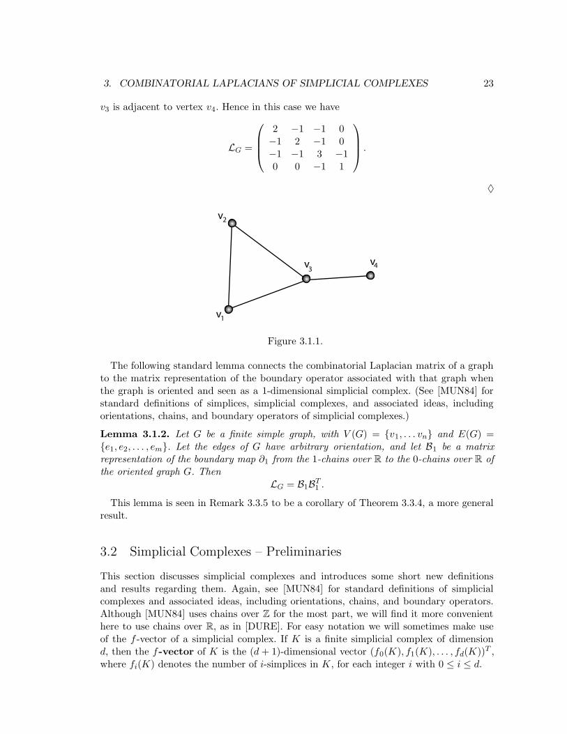
Example 3.1.1. Take the graph from Figure 3.1.1, the border of a triangle with an edgesticking off of one vertex. Vertices v1 and v2 have degree 2, vertex v3 has degree 3, andvertex v4 has degree 1. Vertices v1, v2, and v3 are all adjacent to each other, and vertex
3. COMBINATORIAL LAPLACIANS OF SIMPLICIAL COMPLEXES 23
v3 is adjacent to vertex v4. Hence in this case we have
LG =
2 −1 −1 0−1 2 −1 0−1 −1 3 −10 0 −1 1
.
♦
v
v
vv
1
2
34
Figure 3.1.1.
The following standard lemma connects the combinatorial Laplacian matrix of a graphto the matrix representation of the boundary operator associated with that graph whenthe graph is oriented and seen as a 1-dimensional simplicial complex. (See [MUN84] forstandard definitions of simplices, simplicial complexes, and associated ideas, includingorientations, chains, and boundary operators of simplicial complexes.)
Lemma 3.1.2. Let G be a finite simple graph, with V (G) = {v1, . . . vn} and E(G) ={e1, e2, . . . , em}. Let the edges of G have arbitrary orientation, and let B1 be a matrixrepresentation of the boundary map ∂1 from the 1-chains over R to the 0-chains over R ofthe oriented graph G. Then
LG = B1BT1 .
This lemma is seen in Remark 3.3.5 to be a corollary of Theorem 3.3.4, a more generalresult.
3.2 Simplicial Complexes – Preliminaries
This section discusses simplicial complexes and introduces some short new definitionsand results regarding them. Again, see [MUN84] for standard definitions of simplicialcomplexes and associated ideas, including orientations, chains, and boundary operators.Although [MUN84] uses chains over Z for the most part, we will find it more convenienthere to use chains over R, as in [DURE]. For easy notation we will sometimes make useof the f -vector of a simplicial complex. If K is a finite simplicial complex of dimensiond, then the f-vector of K is the (d + 1)-dimensional vector (f0(K), f1(K), . . . , fd(K))T ,where fi(K) denotes the number of i-simplices in K, for each integer i with 0 ≤ i ≤ d.
3. COMBINATORIAL LAPLACIANS OF SIMPLICIAL COMPLEXES 24
For our purposes, an oriented simplicial complex is one in which all simplices in thecomplex, except for vertices and ∅, are oriented. For any finite simplicial complex K andany nonnegative integer d, the collection of d-chains of K, denoted Cd, is a vector spaceover R. (However, the chains still form a group, and we will follow tradition and refer tothe set of chains of a given dimension as the chain group of that dimension.) A basis forCd is given by the elementary chains associated with the d-simplices of K, so Cd has finitedimension fd(K). Also, if we look at elements of Cd as coordinates relative to this basisof elementary chains, we have the standard inner product on these coordinate vectors,and we see then that this basis of elementary chains is orthonormal. The dth boundaryoperator is a linear transformation Cd −→ Cd−1, and it is denoted ∂d. As is standard, fora simplicial complex of dimension k we define the (−1)-chain group and all chain groupsof dimension greater than k to be the zero vector space.
Definition. Let K be a finite simplicial complex. Two distinct d-simplices σ1, σ2 in K
are upper adjacent, denoted σ1 ∼U σ2, if both are faces of some (d + 1)-simplex τ inK, called their common upper simplex. The upper degree of a d-simplex σ in K,denoted degU (σ), is the number of (d+ 1)-simplices in K of which σ is a face.
Suppose K is oriented, and suppose σ1 and σ2 are d-simplices in K that are upperadjacent with common upper (d+ 1)-simplex τ . We look at the signs of the coefficients ofthese two simplices in the sum ∂d+1(τ). If the signs are the same, we say that σ1 and σ2
are similarly oriented with respect to τ ; if the signs of the coefficients are different, wesay the simplices are dissimilarly oriented. 4
Remark 3.2.1. Note that the equality or inequality of the signs of the coefficients of twoupper adjacent simplices in the sum representing the boundary of their common uppersimplex does not depend on the orientation of the common upper simplex, but only on theorientations of the two upper adjacent simplices. Hence the similarity or dissimilarity oftwo upper adjacent simplices does not depend on the orientation of their common uppersimplex. Also, it is standard to define a 0-simplex, typically called a vertex, as having onlyone choice of orientation. Hence, if two vertices in a simplicial complex are upper adjacent,then they are dissimilarly oriented with respect to their common upper 1-simplex. ♦
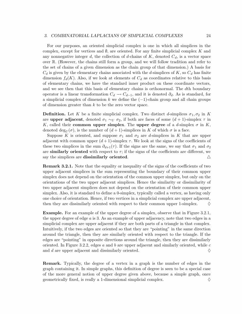
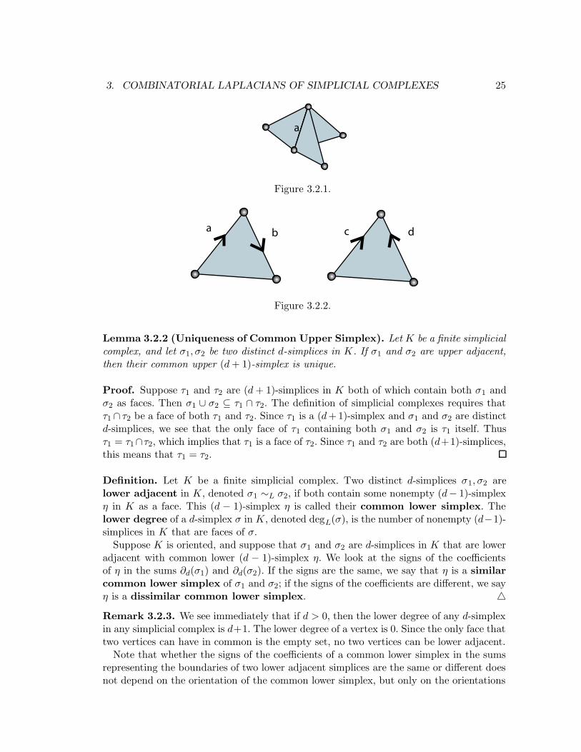
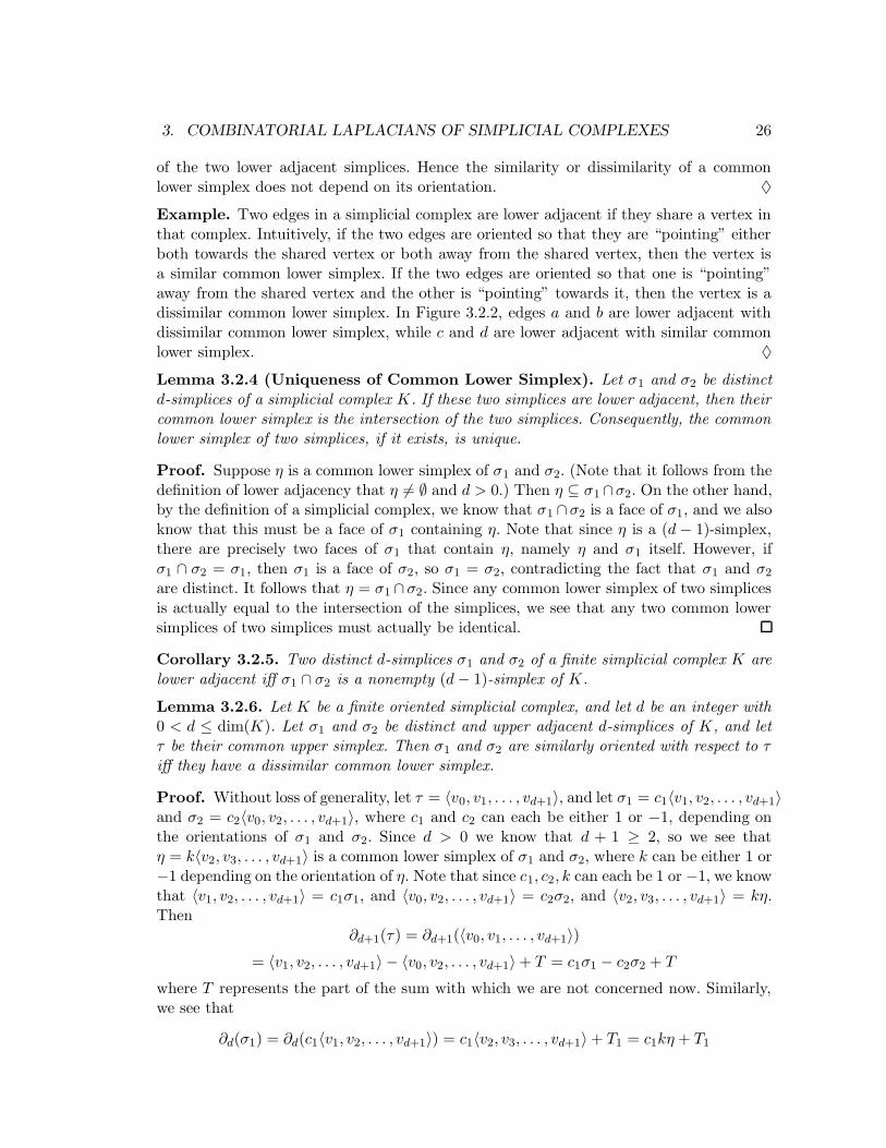
Example. For an example of the upper degree of a simplex, observe that in Figure 3.2.1,the upper degree of edge a is 3. As an example of upper adjacency, note that two edges in asimplicial complex are upper adjacent if they are both parts of a triangle in that complex.Intuitively, if the two edges are oriented so that they are “pointing” in the same directionaround the triangle, then they are similarly oriented with respect to the triangle. If theedges are “pointing” in opposite directions around the triangle, then they are dissimilarlyoriented. In Figure 3.2.2, edges a and b are upper adjacent and similarly oriented, while cand d are upper adjacent and dissimilarly oriented. ♦
Remark. Typically, the degree of a vertex in a graph is the number of edges in thegraph containing it. In simple graphs, this definition of degree is seen to be a special caseof the more general notion of upper degree given above, because a simple graph, oncegeometrically fixed, is really a 1-dimensional simplicial complex. ♦
3. COMBINATORIAL LAPLACIANS OF SIMPLICIAL COMPLEXES 25
a
Figure 3.2.1.
ab c d
Figure 3.2.2.
Lemma 3.2.2 (Uniqueness of Common Upper Simplex). Let K be a finite simplicialcomplex, and let σ1, σ2 be two distinct d-simplices in K. If σ1 and σ2 are upper adjacent,then their common upper (d+ 1)-simplex is unique.
Proof. Suppose τ1 and τ2 are (d+ 1)-simplices in K both of which contain both σ1 andσ2 as faces. Then σ1 ∪ σ2 ⊆ τ1 ∩ τ2. The definition of simplicial complexes requires thatτ1 ∩ τ2 be a face of both τ1 and τ2. Since τ1 is a (d+1)-simplex and σ1 and σ2 are distinctd-simplices, we see that the only face of τ1 containing both σ1 and σ2 is τ1 itself. Thusτ1 = τ1∩τ2, which implies that τ1 is a face of τ2. Since τ1 and τ2 are both (d+1)-simplices,this means that τ1 = τ2.
Definition. Let K be a finite simplicial complex. Two distinct d-simplices σ1, σ2 arelower adjacent in K, denoted σ1 ∼L σ2, if both contain some nonempty (d− 1)-simplexη in K as a face. This (d − 1)-simplex η is called their common lower simplex. Thelower degree of a d-simplex σ in K, denoted degL(σ), is the number of nonempty (d−1)-simplices in K that are faces of σ.
Suppose K is oriented, and suppose that σ1 and σ2 are d-simplices in K that are loweradjacent with common lower (d − 1)-simplex η. We look at the signs of the coefficientsof η in the sums ∂d(σ1) and ∂d(σ2). If the signs are the same, we say that η is a similarcommon lower simplex of σ1 and σ2; if the signs of the coefficients are different, we sayη is a dissimilar common lower simplex. 4Remark 3.2.3. We see immediately that if d > 0, then the lower degree of any d-simplexin any simplicial complex is d+1. The lower degree of a vertex is 0. Since the only face thattwo vertices can have in common is the empty set, no two vertices can be lower adjacent.
Note that whether the signs of the coefficients of a common lower simplex in the sumsrepresenting the boundaries of two lower adjacent simplices are the same or different doesnot depend on the orientation of the common lower simplex, but only on the orientations
3. COMBINATORIAL LAPLACIANS OF SIMPLICIAL COMPLEXES 26
of the two lower adjacent simplices. Hence the similarity or dissimilarity of a commonlower simplex does not depend on its orientation. ♦
Example. Two edges in a simplicial complex are lower adjacent if they share a vertex inthat complex. Intuitively, if the two edges are oriented so that they are “pointing” eitherboth towards the shared vertex or both away from the shared vertex, then the vertex isa similar common lower simplex. If the two edges are oriented so that one is “pointing”away from the shared vertex and the other is “pointing” towards it, then the vertex is adissimilar common lower simplex. In Figure 3.2.2, edges a and b are lower adjacent withdissimilar common lower simplex, while c and d are lower adjacent with similar commonlower simplex. ♦
Lemma 3.2.4 (Uniqueness of Common Lower Simplex). Let σ1 and σ2 be distinctd-simplices of a simplicial complex K. If these two simplices are lower adjacent, then theircommon lower simplex is the intersection of the two simplices. Consequently, the commonlower simplex of two simplices, if it exists, is unique.
Proof. Suppose η is a common lower simplex of σ1 and σ2. (Note that it follows from thedefinition of lower adjacency that η 6= ∅ and d > 0.) Then η ⊆ σ1∩σ2. On the other hand,by the definition of a simplicial complex, we know that σ1 ∩σ2 is a face of σ1, and we alsoknow that this must be a face of σ1 containing η. Note that since η is a (d − 1)-simplex,there are precisely two faces of σ1 that contain η, namely η and σ1 itself. However, ifσ1 ∩ σ2 = σ1, then σ1 is a face of σ2, so σ1 = σ2, contradicting the fact that σ1 and σ2
are distinct. It follows that η = σ1 ∩σ2. Since any common lower simplex of two simplicesis actually equal to the intersection of the simplices, we see that any two common lowersimplices of two simplices must actually be identical.
Corollary 3.2.5. Two distinct d-simplices σ1 and σ2 of a finite simplicial complex K arelower adjacent iff σ1 ∩ σ2 is a nonempty (d− 1)-simplex of K.
Lemma 3.2.6. Let K be a finite oriented simplicial complex, and let d be an integer with0 < d ≤ dim(K). Let σ1 and σ2 be distinct and upper adjacent d-simplices of K, and letτ be their common upper simplex. Then σ1 and σ2 are similarly oriented with respect to τiff they have a dissimilar common lower simplex.
Proof. Without loss of generality, let τ = 〈v0, v1, . . . , vd+1〉, and let σ1 = c1〈v1, v2, . . . , vd+1〉and σ2 = c2〈v0, v2, . . . , vd+1〉, where c1 and c2 can each be either 1 or −1, depending onthe orientations of σ1 and σ2. Since d > 0 we know that d + 1 ≥ 2, so we see thatη = k〈v2, v3, . . . , vd+1〉 is a common lower simplex of σ1 and σ2, where k can be either 1 or−1 depending on the orientation of η. Note that since c1, c2, k can each be 1 or −1, we knowthat 〈v1, v2, . . . , vd+1〉 = c1σ1, and 〈v0, v2, . . . , vd+1〉 = c2σ2, and 〈v2, v3, . . . , vd+1〉 = kη.Then
∂d+1(τ) = ∂d+1(〈v0, v1, . . . , vd+1〉)= 〈v1, v2, . . . , vd+1〉 − 〈v0, v2, . . . , vd+1〉 + T = c1σ1 − c2σ2 + T
where T represents the part of the sum with which we are not concerned now. Similarly,we see that
∂d(σ1) = ∂d(c1〈v1, v2, . . . , vd+1〉) = c1〈v2, v3, . . . , vd+1〉 + T1 = c1kη + T1
3. COMBINATORIAL LAPLACIANS OF SIMPLICIAL COMPLEXES 27
and
∂d(σ2) = ∂d(c2〈v0, v2, . . . , vd+1〉) = c2〈v2, v3, . . . , vd+1〉 + T2 = c2kη + T2
where T1 and T2 represent the unimportant parts of the two sums.(⇒) Suppose σ1 and σ2 are similarly oriented with respect to τ . Then the signs of the
coefficients of these two simplices in the sum ∂d+1(τ) must be the same, so it must bethat c1 = −c2, so c1 and c2 have opposite signs. Then the coefficients of η in ∂d(σ1) and∂d(σ2), which are c1k and c2k, respectively, must have different signs. By definition, thismeans that η is a dissimilar common lower simplex of σ1 and σ2.
(⇐) Suppose σ1 and σ2 are dissimilarly oriented with respect to τ . Then it must bethat c1 and c2 have the same sign, so then c1k and c2k both have the same sign, whichmeans that η is a similar common lower simplex of σ1 and σ2. The contrapositive of thisstatement is, if η is a similar common lower simplex of σ1 and σ2 then σ1 and σ2 aresimilarly oriented with respect to τ .
In the course of the above proof, we proved the following intuitive corollary.
Corollary 3.2.7. Let d > 0 be an integer. If two distinct d-simplices of a finite simplicialcomplex are upper adjacent, then they are also lower adjacent.
3.3 Laplacians of Simplicial Complexes
Note that the matrices of the sole linear operators between trivial vector spaces, from thetrivial vector space to a vector space of dimension n, and from a vector space of dimensionn to the trivial vector space are the 1 × 1 zero matrix, a column vector with n entries allof which are 0, and a row vector with n entries all of which are 0, respectively. (These arethe matrices of the boundary operator ∂d of a simplicial complex K in the cases whered > dim(K) + 1, where d = dim(K) + 1, and where d = 0, respectively.)
For each boundary operator ∂d : Cd −→ Cd−1 ofK, we let Bd be the matrix representationof this operator relative to the standard bases for Cd and Cd−1 with some orderings givento them. We see that the number of rows in Bd is the number of (d − 1)-simplices in K,and the number of columns is the number of d-simplices. Associated with the boundaryoperator ∂d is its adjoint operator ∂∗d : Cd−1 −→ Cd. From [FIS97, Theorem 6.10], weknow that the transpose of the matrix for the dth boundary operator relative to thestandard orthonormal basis of elementary chains with some ordering, BT
d , is the matrixrepresentation of the dth adjoint boundary operator, ∂∗
d with respect to this same orderedbasis.
It is worth noting that the dth adjoint boundary operator of a finite oriented simpli-cial complex K is in fact the same as the dth coboundary operator δd : Cd−1(K; R) −→Cd(K; R) given in [FIS97, page 6], under the isomorphism C d(K; R) = Hom(Cd(K),R) ∼=Cd(K).
The composition of two composable linear maps is a linear map. Two linear maps withidentical domains and codomains can be added by adding their values on any element intheir domain, and the sum of two such maps is clearly another linear map. The followingdefinition comes from [DURE].
3. COMBINATORIAL LAPLACIANS OF SIMPLICIAL COMPLEXES 28
Definition. Let K be a finite oriented simplicial complex, and let d ≥ 0 be an integer.The dth combinatorial Laplacian is the linear operator ∆d : Cd −→ Cd given by
∆d = ∂d+1 ◦ ∂∗d+1 + ∂∗d ◦ ∂d.
For convenience, we use the notations ∆UPd = ∂d+1 ◦ ∂∗d+1 and ∆DN
d = ∂∗d ◦ ∂d, so that
∆d = ∆UPd + ∆DN
d .4
The dth Laplacian matrix ofK, denoted Ld, relative to some orderings of the standardbases for Cd and Cd−1 of K, is the matrix representation of ∆d. Observe that
Ld = Bd+1BTd+1 + BT
d Bd.
As above, for convenience, we use the notations LUPd = Bd+1BT
d+1 and LDNd = BT
d Bd, so
that Ld = LUPd + LDN
d .
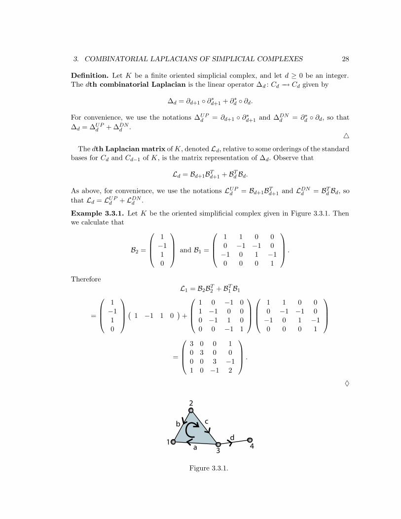
Example 3.3.1. Let K be the oriented simplificial complex given in Figure 3.3.1. Thenwe calculate that
B2 =
1−110
and B1 =
1 1 0 00 −1 −1 0−1 0 1 −10 0 0 1
.
Therefore
L1 = B2BT2 + BT
1 B1
=
1−110
(
1 −1 1 0)
+
1 0 −1 01 −1 0 00 −1 1 00 0 −1 1
1 1 0 00 −1 −1 0−1 0 1 −10 0 0 1
=
3 0 0 10 3 0 00 0 3 −11 0 −1 2
.
♦
a
b c
d1
2
34
Figure 3.3.1.
3. COMBINATORIAL LAPLACIANS OF SIMPLICIAL COMPLEXES 29
Note that ∂0 is the zero map for any simplicial complex, so B0 is a zero matrix. We seethen that ∂∗0 ◦ ∂0 is the zero map, and LDN
0 = BT0 B0 is a zero matrix, so ∆0 = ∂1 ◦ ∂∗1
and L0 = LUPd . Referring back to Lemma 3.1.2, yet to be demonstrated, we see that
our Laplacian matrix for simplicial complexes is a generalization of the combinatorialLaplacian matrix defined in graph theory, because finite simple graphs can be seen assimplicial complexes of dimension 1, embedded in some Euclidean space.
We now present several results that greatly ease the computation of the Laplacian matrixof a simplicial complex.
Proposition 3.3.2. Let K be a finite oriented simplicial complex, and let d be an integerwith 0 ≤ d ≤ dim(K). Let {σ1, σ2, . . . , σn} be the d-simplices of K, and let {τ1, τ2, . . . , τm}be the (d+ 1)-simplices of K. Let i, j ∈ {1, 2, . . . , n}. Then
(LUPd )ij =
degU (σi), if i = j
1, if i 6= j and σi and σj are upper adjacentand oriented similarly
−1, if i 6= j and σi and σj are upper adjacentand oriented dissimilarly
0, if i 6= j and σi and σj are not upper adjacent.
Proof. First, if d = dim(K), then ∂d+1 : Cd+1 −→ Cd is the zero map from the trivialvector space to another vector space, so we see that LUP
d+1 must be a zero matrix. Since inthis case there are no (d + 1)-simplices in K, no d-simplices are upper adjacent in K, sothe proposition follows.
Now, suppose d < dim(K). The ijth component of LUPd+1 = Bd+1B∗
d+1 is the standarddot product of the ith and jth rows of Bd+1. Let X and Y denote these rows, respectively.As before, we will refer to the individual products of the components of X and Y in theirdot product as summands.
Suppose i = j. Let τk be a (d + 1)-simplex in K. If σi is a face of τk, then the kthcomponent of X is either 1 or −1, depending on the orientation of σi, so the kth summandof X ·X is 1. If σi is not a face of τk, then the kth component of X is 0, so the kth summandof X ·X is 0. It follows then that X ·X is the same as the number of (d+ 1)-simplicies inK of which σi is a face, which is of course the upper degree of σi in K.
Suppose i 6= j. Let τk be a (d+1)-simplex in K. Suppose σi and σj are both faces of τk.If σi and σj are similarly oriented, then the kth components of X and Y are either both1 or both −1, so either way the kth summand of X · Y is 1. If σi and σj are dissimilarlyoriented, then of the kth components of X and Y , one is 1 and the other is −1, so thekth summand in X · Y is −1. If σi is not a face of τk, then the kth component of X is 0.Similarly for σj, so if either σi or σj is not a face of τk, then the kth summand of X · Y is0.
We know by Lemma 3.2.2 that there is at most one (d + 1)-simplex in K containingboth σi and σj as faces. Therefore, if σi and σj are upper adjacent, then a single summandof X · Y is either 1 or −1 and all the other summands are 0, so (LUP
d+1)ij = X · Y is either1 or −1, depending on whether the two simplices are oriented similarly or dissimilarly,respectively. If σi and σj are not upper adjacent, then all the summands of X · Y are 0,so (LUP
d+1)ij = X · Y = 0.
3. COMBINATORIAL LAPLACIANS OF SIMPLICIAL COMPLEXES 30
Proposition 3.3.3. Let K be a finite oriented simplicial complex, and let d be an integerwith 0 ≤ d ≤ dim(K). Let {σ1, σ2, . . . , σn} be the d-simplices of K. Let i, j ∈ {1, 2, . . . , n}.Then
(LDNd )ij =
degL(σi), if i = j
1, if i 6= j and σi and σj have a similarcommon lower simplex
−1, if i 6= j and σi and σj have a dissimilarcommon lower simplex
0, if i 6= j and σi and σj are not lower adjacent.
Proof. First, if d = 0, then since ∂0 : C0 −→ C−1 is the zero map from a finite dimensionalvector space to the trivial vector space, we know that LDN
d must be a zero matrix. Sinceno vertices of a simplicial complex are lower adjacent, the proposition follows.
Suppose d > 0. The ijth component of LDNd = B∗
dBd is the standard dot product ofthe ith and jth columns of Bd. Let X and Y denote these columns, respectively, and let{η1, η2, . . . , ηm} be the (d− 1)-simplices of K
Suppose i = j. Let ηk be a (d − 1)-simplex of K. If σi contains ηk as a face, then thekth component of X is either 1 or −1, depending on the orientation of ηk, so the kthsummand of X ·X is 1. If σi does not contain ηk as a face, then the kth component of Xis 0, so the kth summand of X ·X is 0. It follows then that (LDN
d )ij = X ·X is the sameas the number of (d− 1)-faces of σi, which is the lower degree of σi in K.
Suppose i 6= j. Let ηk be a (d − 1)-simplex of K. Suppose σi ∩ σj = ηk, meaning byCorollary 3.2.5 that σi and σj are lower adjacent. If ηk is a similar common lower simplex,then the kth components of X and Y are either both 1 or both −1, so either way thekth summand of X · Y is 1. If ηk is a dissimilar common lower simplex, then of the kthcomponents of X and Y , one is 1 and the other is −1, so the kth summand in X · Y is−1. If ηk is not a face of σi, then the kth component of X is 0. Similarly for σj , so if ηk
is not a common lower simplex of σi and σj , then the kth summand of X · Y is 0.We know by Lemma 3.2.4 that there is at most one (d− 1)-simplex in K that is a face
of both σi and σj. Therefore, if σi and σj have a similar common lower simplex, then asingle summand of X · Y is 1 and all the other summands are 0, so (LDN
d )ij = X · Y = 1.If σi and σj have a dissimilar common lower simplex, then a single summand of X · Y is−1 and all the other summands are 0, so (LDN
d )ij = X · Y = −1. If σi and σj are notlower adjacent, then all the summands of X · Y are 0, so (LDN
d )ij = X · Y = 0.
Theorem 3.3.4 (Laplacian Matrix Theorem). Let K be a finite oriented simplicialcomplex, let d be an integer with 0 ≤ d ≤ dim(K), and let {σ1, σ2, . . . , σn} denote thed-simplices of K. Let i, j ∈ {1, 2, . . . , n}.(1) If d = 0, then
(Ld)ij =
degU(σi), if i = j
−1, if σi and σj are distinct andupper adjacent
0, if σi and σj are distinct andnot upper adjacent.
3. COMBINATORIAL LAPLACIANS OF SIMPLICIAL COMPLEXES 31
(2) If d > 0, then
(Ld)ij =
degU (σi) + d+ 1, if i = j
1, if i 6= j and σi and σj are not upper adjacentbut have a similar common lower simplex
−1, if i 6= j and σi and σj are not upper adjacentbut have a dissimilar common lower simplex
0, if i 6= j and either σi and σj are upper adjacentor are not lower adjacent.
Proof. (1) Suppose d = 0. We remarked at the beginning of this section that L0 = B1BT1 .
In Remark 3.2.1 we noted that since vertices have only one choice of orientation, any twovertices that are upper adjacent are dissimilarly oriented. We see that part (1) of thistheorem follows directly from Proposition 3.3.2.
(2) Suppose d > 0. If i = j, then by Proposition 3.3.2 and Proposition 3.3.3 we know that(Ld)ii = (LUP
d )ii +(LDNd )ii = degU (σi)+degL(σi). Since every simplex of dimension d > 0
has exactly d+ 1 (d− 1)-faces, we see that (Ld)ii = degU (σi) + d+ 1.Suppose i 6= j. If σi and σj are not upper adjacent but have a similar common lower
simplex, then by Proposition 3.3.2 and Proposition 3.3.3 we know that (Ld)ij = (LUPd )ij +
(LDNd )ij = 0 + 1 = 1. If σi and σj are not upper adjacent but have a dissimilar common
lower simplex, then by these same propositions we know that (Ld)ij = (LUPd )ij+(LDN
d )ij =0 + (−1) = −1.
Suppose σi and σj are upper adjacent. If they are similarly oriented, then we knowby Lemma 3.2.6 that they have a dissimilar common lower simplex, so by the same twopropositions used above, we have that (Ld)ij = (LUP
d )ij + (LDNd )ij = 1 + (−1) = 0. On
the other hand, if they are dissimilarly oriented, then they have a similar common lowersimplex, so (Ld)ij = (LUP
d )ij + (LDNd )ij = (−1) + 1 = 0.
Finally, if σj and σi are not lower adjacent, then we know by the contrapositive ofCorollary 3.2.7 that they are not upper adjacent, so then by the same propositions referredto above, we have that (Ld)ij = (LUP
d )ij + (LDNd )ij = 0 + 0 = 0.
The Laplacian Matrix Theorem confirms our calculation of Example 3.3.1. (Or, ourcalculation of Example 3.3.1 confirms the Laplacian Matrix Theorem, depending on yourpoint of view.)
Remark 3.3.5. Since a finite simple graph G can be viewed as a simplicial complex ofdimension 1, we conclude from Theorem 3.3.4 that the matrix LG from the definition inSection 3.1 is the same as the zero Laplacian matrix of G as a simplicial complex. Sincethe definition of the Laplacian matrix of simplicial complexes is in terms of the boundaryoperator, we see that Lemma 3.1.2 follows from Theorem 3.3.4 as a corollary. ♦
Remark 3.3.6. Note that the above theorem implies that the value of the dth Laplacianmatrix of a simplicial complex really depends at most on the orientations of the d-simplicesof the complex, and not on orientations of simplices of other dimensions. ♦
From the Theorem 3.3.4, we deduce the following Corollary. Note that part (1) of thisCorollary is also a formula about the graph theory Laplacian matrix, since the graph
3. COMBINATORIAL LAPLACIANS OF SIMPLICIAL COMPLEXES 32
theory Laplacian is the same as the 0-dimensional Laplacian for simplicial complexes. Theformula in part (1) is a well-known equation in the study of graph theory Laplacians. Itcame from [CHU96, page 317], and served as the inspiration for the formula of part (2).
Corollary 3.3.7. Let K be a finite oriented simplicial complex.
(1) Let v1, . . . , vm be the vertices of K, and let i ∈ {1, . . . ,m}. Then
∆0(vi) =∑
vj∼U vi
(vi − vj).
(2) Let d be an integer with 0 < d ≤ dim(K), let σ1, . . . , σn be the oriented d-simplicesof K, and let i ∈ {1, . . . , n}. Then
∆d(σi) =∑
σj∼Lσi
(σi + sijσj) +∑
σk∼Uσi
(σi − sikσk),
where sij is 1 if σi and σj have a similar common lower simplex, and −1 if theyhave a dissimilar common lower simplex, for all i, j ∈ {1, . . . , n}.
Proof. (1) Theorem 3.3.4 tells us exactly what each entry of L0 looks like, and the vertexvi can be represented by the ith standard basis vector for Rm, which we will denote ei.Then ∆0(vi) is the chain represented by the vector L0ei. This vector is the ith column ofL0, so we see that
∆0(vi) = degU (vi)vi −∑
vj∼Uvi
vj.
The number of j ∈ {1, . . . ,m} − {i} for which vi is upper adjacent to vj is precisely theupper degree of vi, so this formula reduces to
∆0(vi) =∑
vj∼Uvi
(vi − vj).
(2) As in part (1), we see that ∆d(σi) is the chain represented by the vector Ldei, whereei ∈ Rn is the ith standard basis vector. Again, this vector is the ith column of Ld. FromTheorem 3.3.4, we deduce that
∆d(σi) = (degU (σi) + d+ 1)σi +∑
σj∼Lσi
sijσj −∑
σk∼Uσi
sikσk,
because since any two upper adjacent simplices are also lower adjacent, subtracting thetwo sums will cancel all terms containing a simplex σj that is upper adjacent to σi, whichis precisly what is required since the jth entry of the ith column of Ld is 0 if σj is upperadjacent to σi. The coefficients sij account for the signs of the remaining entries, dependingon the similarity or dissimilarity of the relevant common lower simplices. Note that thenumber of σj that are lower adjacent to σi is precisely d+1, and the number of σk that areupper adjacent to σi is precisely degU (σi). Therefore the formula we calculated reduces tothe desired formula, namely
∆d(σi) =∑
σj∼Lσi
(σi + sijσj) +∑
σk∼Uσi
(σi − sikσk).
3. COMBINATORIAL LAPLACIANS OF SIMPLICIAL COMPLEXES 33
Remark 3.3.8. Even though we are using chains over R, the information presented andproved in Section 2.1 shows that all of our work, including defining the Laplacian oper-ator and its matrix, could just as well be done over Z instead. Over Z, the chains of asimplicial complex form a free abelian group, and the boundary operator and Laplacianoperators are both homomorphisms. As detailed in Section 2.1, free abelian groups are al-gebraic structures that are like enough to vector spaces to allow matrix representations ofhomomorphisms between them, and also to define adjoint homomorphisms whose matrixrepresentations are the transposes of the matrices of the original functions.
One reason we use R here is that it allows us to use results from linear algebra directlyon the Laplacian operator, which over R is a linear operator, rather than using thesesame results indirectly on a matrix representation of a homomorphism instead of on thehomomorphism itself. Another very important reason to use vector spaces instead of freeabelian groups is that even though we can define the eigenvalues of a homorphism betweenfree abelian groups to be the eigenvalues of its matrix, the meaning of eigenvalues andeigenvectors for the operator itself may be lost, because the vector representations ofelements of a free abelian group have only integer entries. Any non-integer eigenvalues havelittle of their usual meaning for the homomorphism, and of course non-integer eigenvectorsdo not exist in the chain groups. ♦
3.4 Reduced Laplacians of Simplicial Complexes
Let K be a finite oriented simplicial complex. It is standard to take ∅ to be a (−1)-simplex of K, and suppose that every simplex in K contains ∅ as a face. Normally, theset of (−1)-chains in K is defined to be the trivial vector space. Suppose we define theset of (−1)-chains to be the vector space with singleton basis containing the elementarychain corresponding to ∅. Then this vector space is isomorphic to R. In algebraic topologyit is sometimes useful to regard the (−1)-chain group to be isomorphic to R, and lookat something called the reduced homology groups of K, as in [MUN84]. We will callthe nontrivial vector space of chains with basis {∅} the augmented chain group ofdimension (−1), denoted C̃−1.
In this context, for all integers d > 0 we will speak of the augmented chain group ofdimension d, denoted C̃d, defined to be identical to Cd, the usual chain group of dimensiond. It is also standard to define an augmented boundary operator of dimension 0,denoted ∂̃0 : C̃0 −→ C̃−1, as the linear operator given by ∂̃0(v) = ∅ for all v ∈ C̃0 = C0.Similar to augmented chain groups, for all integers d > 0 we will speak of the augmentedboundary operator of dimension d, denoted ∂̃d, defined to be identical to ∂d, theusual boundary operator of dimension d. Similarly to our nonreduced definitions, theadjoint operator of ∂̃d will be denoted ∂̃∗d . The reduced combinatorial Laplacian of
dimension d, denoted ∆̃d, is the homomorphism from C̃d to C̃d given by
∆̃d = ∂̃d+1 ◦ ∂̃∗d+1 + ∂̃∗d ◦ ∂̃d.
Similarly to the unreduced case, for convenience we use the notations ∆̃UPd = ∂̃d+1∂̃
Td+1
and ∆̃DNd = ∂̃T
d ∂̃d, so that ∆̃d = ∆̃UPd + ∆̃DN
d .
3. COMBINATORIAL LAPLACIANS OF SIMPLICIAL COMPLEXES 34
For all integers d ≥ 0, we let B̃d denote the standard matrix representation of ∂̃d. Asin the unreduced case, we know that B̃T
d is a matrix representation of ∂̃∗d . The reduced
Laplacian matrix of dimension d, denoted L̃d, is the matrix representation of ∆̃d, andwe see that
L̃d = B̃d+1B̃Td+1 + B̃T
d B̃d.
Similarly to the unreduced case, for convenience we use the notations L̃UPd = B̃d+1B̃T
d+1
and L̃DNd = B̃T
d B̃d, so that L̃d = L̃UPd + L̃DN
d .
Remark 3.4.1. Suppose that K contains n vertices. Then B̃0 is a row vector with n
entries all of which are 1. Hence B̃T0 B̃0 is an n×n matrix all of whose entries are 1, which
we denoted Un in Lemma 2.2.9. Then
L̃0 = L0 + Un.
Also, we see immmediately that for any finite oriented simplicial complex K it must bethat ∆̃d = ∆d, and so also L̃d = Ld, for all integers d > 0. ♦
We will now reformulate our definitions and results from Sections 3.2 and 3.3 in termsof reduced Laplacians.
Definition. Let K be a finite simplicial complex. Two distinct d-simplices σ1, σ2 arereduced lower adjacent in K if both contain some (possibly empty) (d− 1)-simplex ηin K as a face. This (d− 1)-simplex η is called their reduced common lower simplex.The reduced lower degree of a d-simplex σ in K, denoted deg �
L(σ), is the number of
(possibly empty) (d− 1)-simplices in K that are faces of σ.Suppose K is oriented and that σ1 and σ2 are d-simplices in K that are lower adjacent
with common lower (d − 1)-simplex η. We look at the signs of the coefficients of η in thesums ∂d(σ1) and ∂d(σ2). If the signs are the same, we say that η is a similar reducedcommon lower simplex of σ1 and σ2; if the signs of the coefficients are different, we sayη is a dissimilar reduced common lower simplex. 4
As before, if d > 0 then the reduced lower degree of any d-simplex in any simplicialcomplex is d + 1; however, now any two vertices have a reduced common lower simplex,namely ∅. Hence, for all integers d ≥ 0, the reduced lower degree of any d-simplex in asimplicial complex is d+ 1. Also, since we assume the empty set has only one orientation,we see that ∅ is a similar reduced common lower simplex of any two vertices in a simplicialcomplex.
For any dimension greater than 0, the concepts of reduced lower adjacency and similaror dissimilar reduced common lower simplices mean exactly the same as their analoguesin un-reduced Laplacians. Concepts of upper adjacency are uneffected when consideringreduced Laplacians.
We will find that the same results that we proved in Section 3.3 in the study of un-reduced Laplacians hold true for the reduced case, except that we gain greater generalityin that all of our results now hold for the 0-dimensional case as well, whereas previouslysome of them did not.
Lemma 3.4.2 (Uniqueness of Reduced Common Lower Simplex). Let σ1 and σ2
be distinct d-simplices of a simplicial complex K. If these two simplices are reduced lower
3. COMBINATORIAL LAPLACIANS OF SIMPLICIAL COMPLEXES 35
adjacent, then their reduced common lower simplex is the intersection of the two simplices.Consequently, the reduced common lower simplex of two simplices, if it exists, is unique.
Proof. For d > 0, the proof of this lemma is the same as for Lemma 3.2.4 in the un-reduced case. If d = 0, then we note that the intersection of any two vertices is the emptyset, which is of course a reduced common lower simplex of the two vertices.
Corollary 3.4.3. Two distinct d-simplices σ1 and σ2 of a finite simplicial complex K arereduced lower adjacent iff σ1 ∩ σ2 is a (d− 1)-simplex of K.
Lemma 3.4.4. Let K be a finite oriented simplicial complex, and let d be an integer with0 ≤ d ≤ dim(K). Let σ1 and σ2 be distinct and upper adjacent d-simplices of K, and letτ be their common upper simplex. Then σ1 and σ2 are similarly oriented with respect to τiff they have a dissimilar reduced common lower simplex.
Proof. If d > 0, the proof is the same as in the un-reduced case in Lemma 3.2.6. Supposed = 0. We know that any two upper adjacent vertices are dissimilarly oriented with respectto their common upper simplex. Since σ1 and σ2 are vertices, we also know that they arereduced lower adjacent, and that the empty set is a similar reduced common lower simplexof them. Since two vertices cannot be similarly oriented with respect to a common uppersimplex, this completes the proof.
We again have the following corollary.
Corollary 3.4.5. Let d ≥ 0 be an integer. If two distinct d-simplices of a finite simplicialcomplex are upper adjacent, then they are also reduced lower adjacent.
Since all definitions for reduced Laplacians are identical to their un-reduced analoguesin any dimension greater than 0, the following proposition is completely equivalent to itsanalogue in the un-reduced case, namely Proposition 3.3.2.
Proposition 3.4.6. Let K be a finite oriented simplicial complex, and let d be an integerwith 0 ≤ d ≤ dim(K). Let {σ1, σ2, . . . , σn} be the d-simplices of K. Let i, j ∈ {1, 2, . . . , n}.Then
(L̃UPd )ij =
degU (σi), if i = j
1, if i 6= j and σi and σj are upper adjacentand oriented similarly
−1, if i 6= j and σi and σj are upper adjacentand oriented dissimilarly
0, if i 6= j and σi and σj are not upper adjacent.
The proof of the next proposition is nearly the same as the proof of Proposition 3.3.3,except that here we can use one proof for all dimensions, instead of different proofs fordimension 0 and dimensions greater than 0.
Proposition 3.4.7. Let K be a finite oriented simplicial complex, and let d be an integerwith 0 ≤ d ≤ dim(K). Let {σ1, σ2, . . . , σn} be the d-simplices of K. Let i, j ∈ {1, 2, . . . , n}.Then
3. COMBINATORIAL LAPLACIANS OF SIMPLICIAL COMPLEXES 36
(L̃DNd )ij =
deg �
L(σi), if i = j
1, if i 6= j and σi and σj have a similarreduced common lower simplex
−1, if i 6= j and σi and σj have a dissimilarreduced common lower simplex
0, if i 6= j and σi and σj are not reduced lower adjacent.
Proof. If d > 0, then the proof is the same as the proof of its un-reduced analogue,Proposition 3.3.3. Suppose d = 0. Every vertex contains exactly one (−1)-face, the emptyset, so the reduced lower degree of any vertex is 1. Any two distinct vertices are reducedlower adjacent, and the empty set is a similar reduced common lower simplex of them.From Remark 3.4.1, we know that B̃T
0 B̃0 is a matrix whose entries are all 1. This provesthe proposition.
Propositions 3.4.6 and 3.4.7 look very much like their unreduced counterparts, but theReduced Laplacian Matrix Theorem is clearly slightly different, and essentially tidier, thanits unreduced counterpart, the Laplacian Matrix Theorem.
Theorem 3.4.8 (Reduced Laplacian Matrix Theorem). Let K be a finite orientedsimplicial complex, and let d be an integer with 0 ≤ d ≤ dim(K), and let {σ1, σ2, . . . , σn}denote the d-simplices of K. Let i, j ∈ {1, 2, . . . , n}. Then
(L̃d)ij =
degU (σi) + d+ 1, if i = j
1, if i 6= j and σi and σj are not upper adjacentbut have a similar reduced common lower simplex
−1, if i 6= j and σi and σj are not upper adjacentbut have a dissimilar reduced common lower simplex
0, if i 6= j and either σi and σj are upper adjacentor are not reduced lower adjacent.
Proof. The proof of this theorem is identical to the proof of part (ii) of this theorem’sun-reduced analogue, Theorem 3.3.4, which proves the theorem if d > 0. The only reasonthe same argument did not apply previously if d = 0 is that it relied on results that werenot true for d = 0, namely Corollary 3.2.7 and Lemmas 3.2.6 and 3.3.3. However, in thereduced case, the analogues of these results, namely Corollary 3.4.5 and Lemmas 3.4.4and 3.4.7, hold true for all integers d ≥ 0.
Again, we have the following Corollary. The proof of this result is identical to the proofof Corollary 3.3.7 (2).
Corollary 3.4.9. Let K be a finite oriented simplicial complex. Let d be an integer with0 ≤ d ≤ dim(K), let σ1, . . . , σn be the oriented d-simplices of K, and let i ∈ {1, . . . , n}.Then
∆̃d(σi) =∑
σj∼L̃σi
(σi + sijσj) +∑
σk∼Uσi
(σi − sikσk),
3. COMBINATORIAL LAPLACIANS OF SIMPLICIAL COMPLEXES 37
where sij is 1 if σi and σj have a similar reduced common lower simplex, and −1 if theyhave a dissimilar reduced common lower simplex, for all i, j ∈ {1, . . . , n}.
4Laplacian Spectra of Simplicial Complexes
4.1 Spectra of ∆, ∆̃, ∆UP , and ∆DN
We now present some extremely useful and pretty results about the eigenvalues of Lapla-cian operators.
Definition. Let K be a finite oriented simplicial complex, and let d be an integer with0 ≤ d ≤ dim(K). Then the dth Laplacian spectrum of K, denoted Spec(∆d(K)), is themultiset of eigenvalues of ∆d of K. 4Theorem 4.1.1. Let K be a finite simplicial complex, and let d be an integer with 0 ≤ d ≤dimK. Then Spec(∆d(K)) is independent of the choice of orientation for the d-simplicesof that complex.
Proof. By Theorem 3.3.4, it is apparent that the diagonal entries of a Laplacian matrixare independent of orientation, and similarly we note that whether a nondiagonal entryis zero or nonzero is independent of orientation as well. So, we see that only the signs ofthe nonzero nondiagonal entries of the Laplacian matrix are dependent on orientation. Ifd = 0, then this is not an issue, since all nondiagonal entries of L0 are either 0 or −1 forany simplicial complex.
Suppose d > 0. Let {σ1, σ2, . . . , σn} denote the d-simplices of K. Suppose K1 is thesimplicial complex K with some arbitrary orientation given to the d-simplices, and thatK2 is also the complex K with the same orientations on the d-simplices as in K1 exceptthat σp has the opposite orientation in K2 as it does in K1, for some p ∈ {1, 2, . . . , n}. LetLd(K1) and Ld(K2) denote the dth Laplacian matrices of K1 and K2, respectively. Let σp
denote the elementary chain of this simplex with respect to its orientation given in K1,and then −σp will denote the elementary chain of this same simplex with respect to itsorientation given in K2.
Suppose σi is lower but not upper adjacent with σp. Let η be the common lower simplexof σi and σp. Note that ∂d(−σp) = −∂d(σp), so the coefficient of η in ∂d(−σp) has the
4. LAPLACIAN SPECTRA OF SIMPLICIAL COMPLEXES 39
opposite sign from its sign in ∂d(σp). Hence, if the coefficient of η in ∂d(σi) has thesame sign as its coefficient in ∂d(σp), then the coefficient in ∂d(σi) has the opposite signas its coefficient in ∂d(−σp). Similarly, if the coefficient of η in ∂d(σi) has the oppositesign as its coefficient in ∂d(σp), then the coefficient in ∂d(σi) has the same sign as itscoefficient in ∂d(−σp). Therefore if σp and σi have a similar common lower simplex in K1,then they have a dissimilar common lower simplex in K2, and vice versa. It follows that(Ld(K1))pi = (Ld(K1))ip has the opposite sign of (Ld(K2))pi = (Ld(K2))ip.
Since this holds true for any σi with which σp is lower but not upper adjacent, we seethat Ld(K2) is the same as Ld(K1) except that every nondiagonal nonzero entry in rowp or in column p has the opposite sign. This result can be obtained by multiplying eachentry in row p by −1 and then multiplying each entry in column p by −1, because thiswill not affect any zero entries, and the pth diagonal entry will be multiplied by −1 twice,leaving it alone.
For each x ∈ {1, 2, . . . , n} let Jx denote the n× n matrix given by
(Jx)ij =
−1, if i = x = j
1, if x 6= i = j
0, otherwise.
For all x ∈ {1, 2, . . . , n} note that Jx is invertible and is in fact idempotent. Also, notethat for any n× n matrix A, multiplication on the left by Jx will yield a matrix identicalto A except with all the entries in row x multiplied by −1, and multiplication by Jx onthe right yields a matrix identical to A except with all the entries in column x multipliedby −1.
We see then that Ld(K2) = JpLd(K1)Jp. Since Jp is idempotent, this means thatLd(K2) and Ld(K1) are similar matrices. A well-known result in linear algebra statesthat similar matrices have identical eigenvalues, (see [FIS97, page 240]), so it follows thatSpec(∆d(K1)) = Spec(∆d(K2)).
The above argument dealt with the case where the orientation of simplices of a particulardimension in two geometrically identical finite simplicial complexes differed only in theorientation of a single simplex. Since we are dealing with finite simplicial complexes, thecomplete result of this theorem follows by a simple application of mathematical induction.
Example 4.1.2. In Figure 4.1.1, we have two oriented simplicial complexes K1 and K2
that are geometrically identical but have different orientations on their simplices. Wecalculate that
L1(K1) =
3 0 0 00 3 0 −10 0 3 −10 −1 −1 2
and L1(K2) =
3 0 0 00 3 0 −10 0 3 10 −1 1 2
,
but Spec(∆1(K1)) = {1, 3, 3, 4} = Spec(∆1(K2)). ♦
Definition. Let K be a finite oriented simplicial complex, and let d be an integer with 0 ≤d ≤ dim(K). Then the dth reduced Laplacian spectrum of K, denoted Spec(∆̃d(K)),is the multiset of eigenvalues of ∆̃d of K. 4
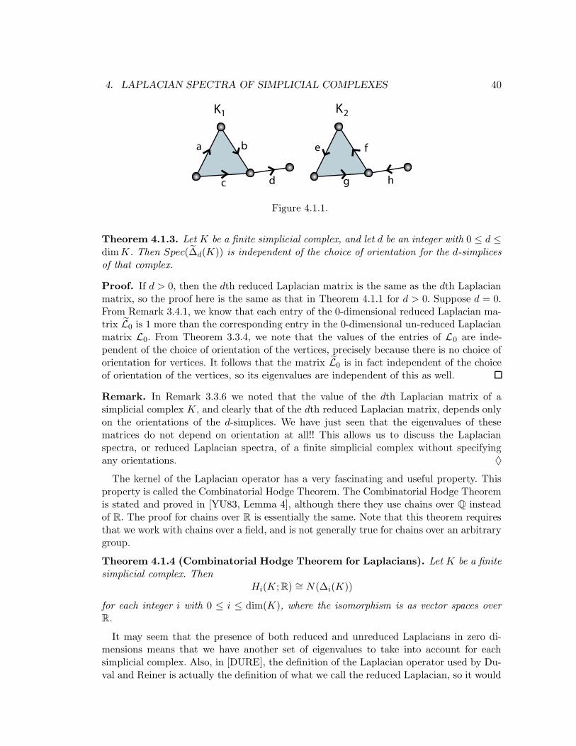
4. LAPLACIAN SPECTRA OF SIMPLICIAL COMPLEXES 40
a b
c d
1K
e f
2K
g h
Figure 4.1.1.
Theorem 4.1.3. Let K be a finite simplicial complex, and let d be an integer with 0 ≤ d ≤dimK. Then Spec(∆̃d(K)) is independent of the choice of orientation for the d-simplicesof that complex.
Proof. If d > 0, then the dth reduced Laplacian matrix is the same as the dth Laplacianmatrix, so the proof here is the same as that in Theorem 4.1.1 for d > 0. Suppose d = 0.From Remark 3.4.1, we know that each entry of the 0-dimensional reduced Laplacian ma-trix L̃0 is 1 more than the corresponding entry in the 0-dimensional un-reduced Laplacianmatrix L0. From Theorem 3.3.4, we note that the values of the entries of L0 are inde-pendent of the choice of orientation of the vertices, precisely because there is no choice oforientation for vertices. It follows that the matrix L̃0 is in fact independent of the choiceof orientation of the vertices, so its eigenvalues are independent of this as well.
Remark. In Remark 3.3.6 we noted that the value of the dth Laplacian matrix of asimplicial complex K, and clearly that of the dth reduced Laplacian matrix, depends onlyon the orientations of the d-simplices. We have just seen that the eigenvalues of thesematrices do not depend on orientation at all!! This allows us to discuss the Laplacianspectra, or reduced Laplacian spectra, of a finite simplicial complex without specifyingany orientations. ♦
The kernel of the Laplacian operator has a very fascinating and useful property. Thisproperty is called the Combinatorial Hodge Theorem. The Combinatorial Hodge Theoremis stated and proved in [YU83, Lemma 4], although there they use chains over Q insteadof R. The proof for chains over R is essentially the same. Note that this theorem requiresthat we work with chains over a field, and is not generally true for chains over an arbitrarygroup.
Theorem 4.1.4 (Combinatorial Hodge Theorem for Laplacians). Let K be a finitesimplicial complex. Then
Hi(K; R) ∼= N(∆i(K))
for each integer i with 0 ≤ i ≤ dim(K), where the isomorphism is as vector spaces overR.
It may seem that the presence of both reduced and unreduced Laplacians in zero di-mensions means that we have another set of eigenvalues to take into account for eachsimplicial complex. Also, in [DURE], the definition of the Laplacian operator used by Du-val and Reiner is actually the definition of what we call the reduced Laplacian, so it would
4. LAPLACIAN SPECTRA OF SIMPLICIAL COMPLEXES 41
be nice if there is some easy way to convert between their Laplacian spectra and ours,even though reduced and unreduced Laplacians are only different in the case of dimension0. The following result makes this connection.
Theorem 4.1.5. Let K be a finite simplicial complex with n vertices. Then
SpecNZ(∆̃0(K)) = SpecNZ(∆0(K)) ∪M {n},
andSpec(∆̃d(K)) = Spec(∆d(K))
for all integers d > 0.
Proof. The second equation in the statement of the theorem follows from the fact thatfor all integers d > 0 we have ∆d(K) = ∆̃d(K).
For the first equation, let {v1, v2, . . . , vn} denote the vertices of K. Recall the definitionof Un from Lemma 2.2.9. By Remark 3.4.1 we know that L̃0 = L0 + Un. We will showthat L0Un and UnL0 are both the n× n zero matrix, so that ∆0 and the linear operatorC0 −→ C0 represented by Un are mutually annihilating operators.
Let i, j ∈ {1, 2, . . . , n}. Making use of Theorem 3.3.4, we see that the ijth componentof L0Un is the sum of the components of the ith row of L0, which is
n∑
j=1
(L0)ij = degU vi +∑
vk∼Uvi
(−1).
Since the upper degree of a vertex is precisely the number of vertices with which it isupper adjacent, we see that this sum and hence this component must be 0. Similarly, theijth component of UnL0 is the sum of the components of the jth row of L0, which is
n∑
i=1
(L0)ij = degU vj +∑
vk∼Uvj
(−1),
which must also be 0.Since ∆0 and the operator given by Un are self-adjoint as well as mutually annihilat-
ing, it follows by Theorem 2.2.5 that SpecNZ(L0 + Un) = SpecNZ(L0) ∪M SpecNZ(Un).From Lemma 2.2.9 we know that SpecNZ(Un) = {n}. Therefore SpecNZ(∆̃0(K)) =SpecNZ(∆0(K)) ∪M {n}.
In the case of a connected complex, Theorem 4.1.5 can be made even more specific,describing the actual spectra instead of the non-zero spectra.
Corollary 4.1.6. Let K be a connected finite simplicial complex with n vertices. Then
Spec(∆̃0(K)) = SpecNZ(∆0(K)) ∪M {n}.
Proof. From Theorem 4.1.4, we know that the dimension of the nullspace of ∆0, whichis the multiplicity of 0 as an eigenvalue of ∆0, is the dimension of the 0th homology groupof K. It is well known [MUN84, Theorem 7.1] that the dimension of the 0th homologygroup of K is equal to the number of components of K, which in this case is 1. Therefore
4. LAPLACIAN SPECTRA OF SIMPLICIAL COMPLEXES 42
0 is an eigenvalue of multiplicity 1 of ∆0(K), so ∆0(K) has precisely n − 1 nonzeroeigenvalues. Since ∆̃0(K) can have only n eigenvalues, by Theorem 4.1.5 we see thatSpec(∆̃0(K)) = SpecNZ(∆0(K)) ∪M {n}.
The following lemma describes the very useful relationship between the spectrum of ∆,and the spectra of ∆UP and ∆DN , in both non-reduced and reduced settings.
Lemma 4.1.7. Let K be a finite oriented simplicial complex, and let d ∈ Z be such that0 ≤ d ≤ dim(K). Then
SpecNZ(∆d(K)) = SpecNZ(∆UPd (K)) ∪M SpecNZ(∆DN
d (K))
andSpecNZ(∆̃d(K)) = SpecNZ(∆̃UP
d (K)) ∪M SpecNZ(∆̃DNd (K)).
Proof. As linear operators, we know that both ∆UPd and ∆DN
d are self-adjoint. From[MUN84, Lemma 5.3] we know that the image of the boundary operator of a given dimen-sion is contained in the nullspace of the boundary operator of the next lower dimension,and from [FIS97, Theorem 6.11 (c)] we know that the adjoint of the composition of twolinear operators is the composition in the opposite direction of the adjoints of the twooperators. Also, we see easily that the composition on either side of a linear operator withthe zero map of the proper dimension is the zero map of the proper dimension, and thatthe adjoint of a zero map is another zero map. Taken altogether, these facts imply that
∆UPd ◦ ∆DN
d = (∂d+1 ◦ ∂∗d+1) ◦ (∂∗d ◦ ∂d) = ∂d+1 ◦ (∂∗d+1 ◦ ∂∗d) ◦ ∂d
= ∂d+1 ◦ (∂d ◦ ∂d+1)∗ ◦ ∂d = ∂d+1 ◦ 0∗ ◦ ∂d
= ∂d+1 ◦ 0 ◦ ∂d = 0.
In a similar fashion, we have
∆DNd ◦ ∆UP
d = (∂∗d ◦ ∂d) ◦ (∂d+1 ◦ ∂∗d+1) = ∂∗d ◦ (∂d ◦ ∂d+1) ◦ ∂∗d+1
= ∂∗d ◦ 0 ◦ ∂∗d+1 = 0.
Therefore ∆UPd and ∆DN
d are self-adjoint, mutually annihilating operators. Similarly for
∆̃UPd and ∆̃DN
d . The desired results follow directly from Theorem 2.2.5.
This next lemma displays the relationship between the spectra of ∆UP and ∆DN , againin both nonreduced and reduced settings.
Lemma 4.1.8. Let K be a finite simplicial complex. Then
SpecNZ(∆UPd−1(K)) = SpecNZ(∆DN
d (K))
andSpecNZ(∆̃UP
d−1(K)) = SpecNZ(∆̃DNd (K))
for all positive integers d ≤ dim(K).
Proof. Since ∆UPd−1 = ∂d∂
∗d and ∆DN
d = ∂∗d∂d, and ∆̃UPd−1 = ∂̃d∂̃
∗d and ∆̃DN
d = ∂̃∗d ∂̃d, theseresults follow immediately from Theorem 2.2.6.
4. LAPLACIAN SPECTRA OF SIMPLICIAL COMPLEXES 43
As remarked in [DURE, page 9], it is seen from Lemmas 4.1.7 and 4.1.8 that for a finitesimplicial complex the information carried by the spectra of ∆, the spectra of ∆UP , andthe spectra of ∆DN is essentially the same. Hence, in studying the Laplacian spectra wecan feel free to study the spectra of whichever of these three families of operators is mostconvenient.
In 2 dimensions, we have this corollary, which is simply a special case of Lemma 4.1.7.
Corollary 4.1.9. Let K be a finite simplicial complex of dimension 2. Then
SpecNZ(∆1(K)) = SpecNZ(∆0(K)) ∪M SpecNZ(∆2(K)).
Proof. Note that Spec(∆0(K)) = Spec(∆UP0 (K)) and Spec(∆2(K)) = Spec(∆DN
2 (K)),because K is 2-dimensional. Then by Lemmas 4.1.7 and 4.1.8, respectively, we haveSpecNZ(∆1(K)) = SpecNZ(∆DN
1 (K)) ∪M SpecNZ(∆UP1 (K)) = SpecNZ(∆UP
0 (K)) ∪M
SpecNZ(∆DN2 (K)) = SpecNZ(∆0(K)) ∪M SpecNZ(∆2(K)).
4.2 Further Facts about Laplacian Spectra
Since the Laplacian matrix is the sum of compositions of linear operators with theiradjoints, it is self-adjoint. By Theorem 6.17 and the lemma preceding it in [FIS97], weknow that the Laplacian matrix is diagonalizable and that all of its eigenvalues are real.From Lemmas 2.2.8 and 2.2.7, we know that the Laplacian operator is positive semidefinite,and has only nonnegative eigenvalues. The following result goes even further, and presentssome good news for people who do not like fractions, (or bad news for people who likethem).
Theorem 4.2.1. Let K be a finite simplicial complex, and let i be an integer with 0 ≤i ≤ dim(K). Then Spec(∆i(K)) contains no non-integer rational numbers.
Proof. The eigenvalues of ∆i(K) are the roots of its characteristic polynomial f(t) =det(Li(K)− tIfi(K)), where Li(K) is the matrix of ∆i(K) relative to an arbitrary orderingand orientation of the i-simplices ofK, and Ifi(K)) is the fi(K)×fi(K) identity matrix. Weknow by Theorem 3.3.4 that Li(K) is an integer matrix, so it is easy to deduce that f(t) isa polynomial over the integers. By [FIS97, Theorem 5.8], we know that the lead coefficientof f(t) is (−1)fi(K). By the Rational Roots Theorem ([AMB77, Theorem 13.10]), we knowthat the denominator of any rational root of a polynomial over the integers must be afactor of the lead coefficient of that polynomial. Hence the only rational roots of f(t) havedenominator divisible by ±1, so they are integers. Therefore the only roots of f(t) areintegers or irrational numbers.
Example 4.2.2. Even though Laplacian spectra do not contain fractions, they candefinitely contain lots of irrational numbers. By the Laplacian Matrix Theorem, Theo-rem 3.3.4, we can calculate that for the simplicial complex K in Figure 4.2.1 we havethat Spec(∆0(K)) consists of 0, 1
2(7 ±√
13), and the three roots of the cubic polynomialx3 −9x2 +23x−14, which are approximately 0.885092, 3.2541, 4.86081. Also, we calculatethat
Spec(∆2(K)) = {3, 3 ±√
2}.
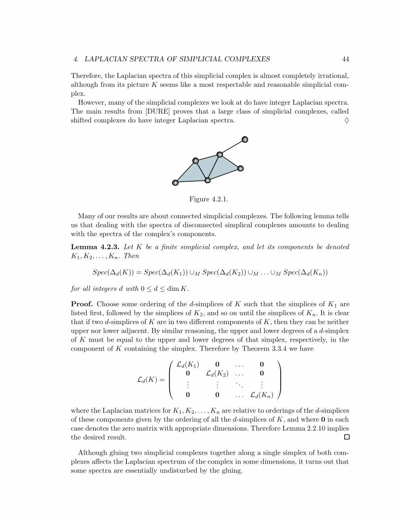
4. LAPLACIAN SPECTRA OF SIMPLICIAL COMPLEXES 44
Therefore, the Laplacian spectra of this simplicial complex is almost completely irrational,although from its picture K seems like a most respectable and reasonable simplicial com-plex.
However, many of the simplicial complexes we look at do have integer Laplacian spectra.The main results from [DURE] proves that a large class of simplicial complexes, calledshifted complexes do have integer Laplacian spectra. ♦
Figure 4.2.1.
Many of our results are about connected simplicial complexes. The following lemma tellsus that dealing with the spectra of disconnected simplical complexes amounts to dealingwith the spectra of the complex’s components.
Lemma 4.2.3. Let K be a finite simplicial complex, and let its components be denotedK1,K2, . . . ,Kn. Then
Spec(∆d(K)) = Spec(∆d(K1)) ∪M Spec(∆d(K2)) ∪M . . . ∪M Spec(∆d(Kn))
for all integers d with 0 ≤ d ≤ dimK.
Proof. Choose some ordering of the d-simplices of K such that the simplices of K1 arelisted first, followed by the simplices of K2, and so on until the simplices of Kn. It is clearthat if two d-simplices of K are in two different components of K, then they can be neitherupper nor lower adjacent. By similar reasoning, the upper and lower degrees of a d-simplexof K must be equal to the upper and lower degrees of that simplex, respectively, in thecomponent of K containing the simplex. Therefore by Theorem 3.3.4 we have
Ld(K) =
Ld(K1) 0 . . . 00 Ld(K2) . . . 0...
.... . .
...0 0 . . . Ld(Kn)
where the Laplacian matrices forK1,K2, . . . ,Kn are relative to orderings of the d-simplicesof these components given by the ordering of all the d-simplices of K, and where 0 in eachcase denotes the zero matrix with appropriate dimensions. Therefore Lemma 2.2.10 impliesthe desired result.
Although gluing two simplicial complexes together along a single simplex of both com-plexes affects the Laplacian spectrum of the complex in some dimensions, it turns out thatsome spectra are essentially undisturbed by the gluing.
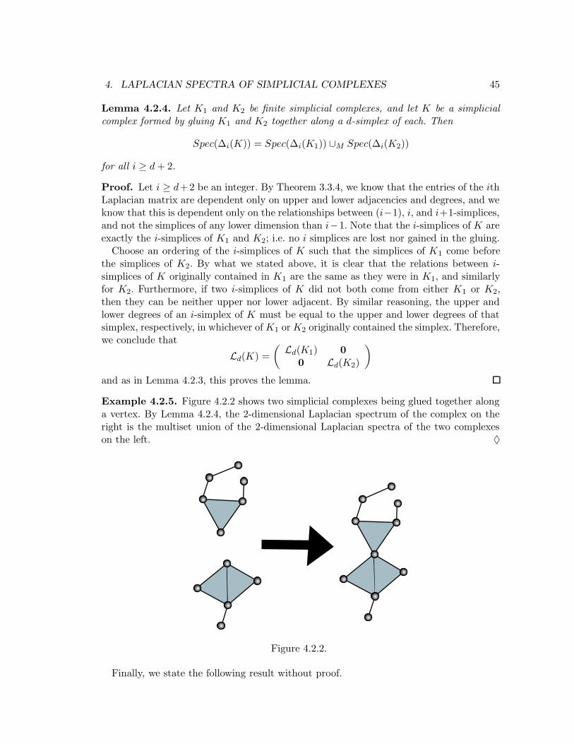
4. LAPLACIAN SPECTRA OF SIMPLICIAL COMPLEXES 45
Lemma 4.2.4. Let K1 and K2 be finite simplicial complexes, and let K be a simplicialcomplex formed by gluing K1 and K2 together along a d-simplex of each. Then
Spec(∆i(K)) = Spec(∆i(K1)) ∪M Spec(∆i(K2))
for all i ≥ d+ 2.
Proof. Let i ≥ d+2 be an integer. By Theorem 3.3.4, we know that the entries of the ithLaplacian matrix are dependent only on upper and lower adjacencies and degrees, and weknow that this is dependent only on the relationships between (i−1), i, and i+1-simplices,and not the simplices of any lower dimension than i−1. Note that the i-simplices of K areexactly the i-simplices of K1 and K2; i.e. no i simplices are lost nor gained in the gluing.
Choose an ordering of the i-simplices of K such that the simplices of K1 come beforethe simplices of K2. By what we stated above, it is clear that the relations between i-simplices of K originally contained in K1 are the same as they were in K1, and similarlyfor K2. Furthermore, if two i-simplices of K did not both come from either K1 or K2,then they can be neither upper nor lower adjacent. By similar reasoning, the upper andlower degrees of an i-simplex of K must be equal to the upper and lower degrees of thatsimplex, respectively, in whichever ofK1 orK2 originally contained the simplex. Therefore,we conclude that
Ld(K) =
(Ld(K1) 0
0 Ld(K2)
)
and as in Lemma 4.2.3, this proves the lemma.
Example 4.2.5. Figure 4.2.2 shows two simplicial complexes being glued together alonga vertex. By Lemma 4.2.4, the 2-dimensional Laplacian spectrum of the complex on theright is the multiset union of the 2-dimensional Laplacian spectra of the two complexeson the left. ♦
Figure 4.2.2.
Finally, we state the following result without proof.
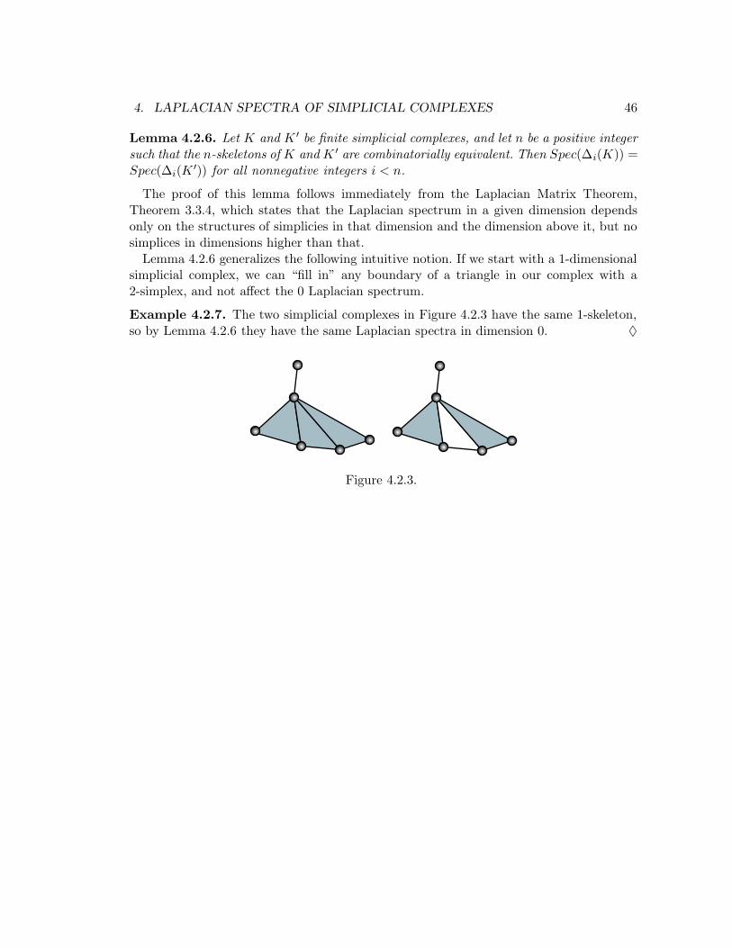
4. LAPLACIAN SPECTRA OF SIMPLICIAL COMPLEXES 46
Lemma 4.2.6. Let K and K ′ be finite simplicial complexes, and let n be a positive integersuch that the n-skeletons of K and K ′ are combinatorially equivalent. Then Spec(∆i(K)) =Spec(∆i(K
′)) for all nonnegative integers i < n.
The proof of this lemma follows immediately from the Laplacian Matrix Theorem,Theorem 3.3.4, which states that the Laplacian spectrum in a given dimension dependsonly on the structures of simplicies in that dimension and the dimension above it, but nosimplices in dimensions higher than that.
Lemma 4.2.6 generalizes the following intuitive notion. If we start with a 1-dimensionalsimplicial complex, we can “fill in” any boundary of a triangle in our complex with a2-simplex, and not affect the 0 Laplacian spectrum.
Example 4.2.7. The two simplicial complexes in Figure 4.2.3 have the same 1-skeleton,so by Lemma 4.2.6 they have the same Laplacian spectra in dimension 0. ♦
Figure 4.2.3.
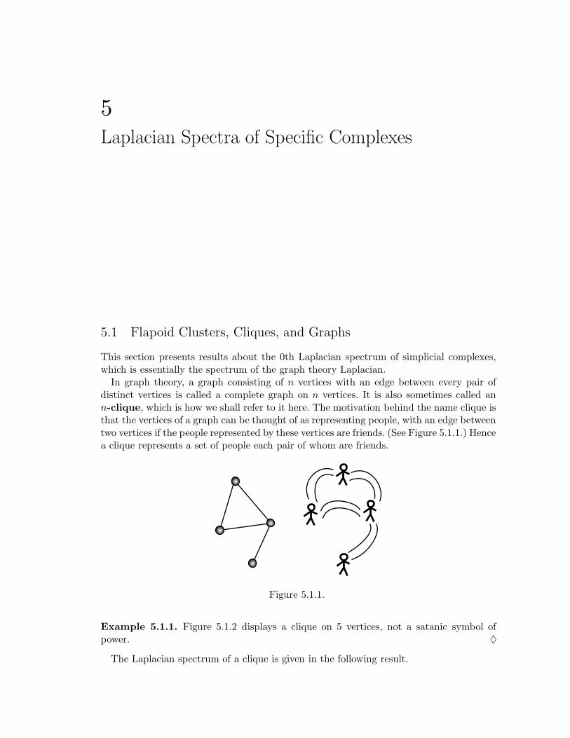
5Laplacian Spectra of Specific Complexes
5.1 Flapoid Clusters, Cliques, and Graphs
This section presents results about the 0th Laplacian spectrum of simplicial complexes,which is essentially the spectrum of the graph theory Laplacian.
In graph theory, a graph consisting of n vertices with an edge between every pair ofdistinct vertices is called a complete graph on n vertices. It is also sometimes called ann-clique, which is how we shall refer to it here. The motivation behind the name clique isthat the vertices of a graph can be thought of as representing people, with an edge betweentwo vertices if the people represented by these vertices are friends. (See Figure 5.1.1.) Hencea clique represents a set of people each pair of whom are friends.
Figure 5.1.1.
Example 5.1.1. Figure 5.1.2 displays a clique on 5 vertices, not a satanic symbol ofpower. ♦
The Laplacian spectrum of a clique is given in the following result.
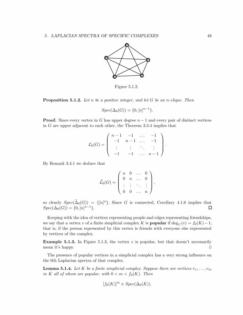
5. LAPLACIAN SPECTRA OF SPECIFIC COMPLEXES 48
Figure 5.1.2.
Proposition 5.1.2. Let n be a positive integer, and let G be an n-clique. Then
Spec(∆0(G)) = {0, [n]n−1}.
Proof. Since every vertex in G has upper degree n− 1 and every pair of distinct verticesin G are upper adjacent to each other, the Theorem 3.3.4 implies that
L0(G) =
n− 1 −1 . . . −1−1 n− 1 . . . −1...
.... . .
...−1 −1 . . . n− 1
.
By Remark 3.4.1 we deduce that
L̃0(G) =
n 0 . . . 00 n . . . 0...
.... . .
...0 0 . . . n
,
so clearly Spec(∆̃0(G)) = {[n]n}. Since G is connected, Corollary 4.1.6 implies thatSpec(∆0(G)) = {0, [n]n−1}.
Keeping with the idea of vertices representing people and edges representing friendships,we say that a vertex v of a finite simplicial complex K is popular if degU (v) = f0(K)−1;that is, if the person represented by this vertex is friends with everyone else representedby vertices of the complex.
Example 5.1.3. In Figure 5.1.3, the vertex v is popular, but that doesn’t necessarilymean it’s happy. ♦
The presence of popular vertices in a simplicial complex has a very strong influence onthe 0th Laplacian spectra of that complex.
Lemma 5.1.4. Let K be a finite simplicial complex. Suppose there are vertices v1, . . . , vm
in K all of whom are popular, with 0 < m < f0(K). Then
[f0(K)]m ∈ Spec(∆0(K)).
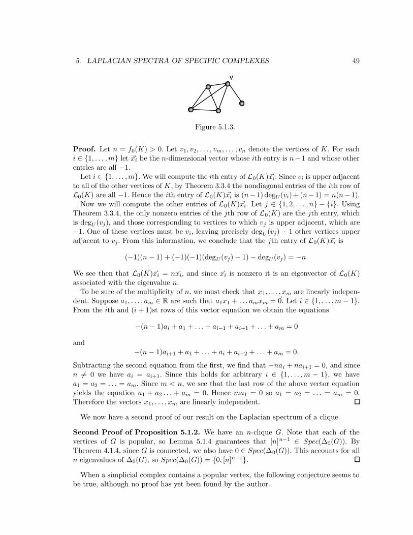
5. LAPLACIAN SPECTRA OF SPECIFIC COMPLEXES 49
v
Figure 5.1.3.
Proof. Let n = f0(K) > 0. Let v1, v2, . . . , vm, . . . , vn denote the vertices of K. For eachi ∈ {1, . . . ,m} let ~xi be the n-dimensional vector whose ith entry is n−1 and whose otherentries are all −1.
Let i ∈ {1, . . . ,m}. We will compute the ith entry of L0(K)~xi. Since vi is upper adjacentto all of the other vertices of K, by Theorem 3.3.4 the nondiagonal entries of the ith row ofL0(K) are all −1. Hence the ith entry of L0(K)~xi is (n− 1) degU (vi)+ (n− 1) = n(n− 1).
Now we will compute the other entries of L0(K)~xi. Let j ∈ {1, 2, . . . , n} − {i}. UsingTheorem 3.3.4, the only nonzero entries of the jth row of L0(K) are the jth entry, whichis degU (vj), and those corresponding to vertices to which vj is upper adjacent, which are−1. One of these vertices must be vi, leaving precisely degU (vj) − 1 other vertices upperadjacent to vj. From this information, we conclude that the jth entry of L0(K)~xi is
(−1)(n− 1) + (−1)(−1)(degU (vj) − 1) − degU (vj) = −n.
We see then that L0(K)~xi = n~xi, and since ~xi is nonzero it is an eigenvector of L0(K)associated with the eigenvalue n.
To be sure of the multiplicity of n, we must check that x1, . . . , xm are linearly indepen-dent. Suppose a1, . . . , am ∈ R are such that a1x1 + . . . amxm = ~0. Let i ∈ {1, . . . ,m− 1}.From the ith and (i+ 1)st rows of this vector equation we obtain the equations
−(n− 1)ai + a1 + . . .+ ai−1 + ai+1 + . . .+ am = 0
and−(n− 1)ai+1 + a1 + . . . + ai + ai+2 + . . . + am = 0.
Subtracting the second equation from the first, we find that −nai + nai+1 = 0, and sincen 6= 0 we have ai = ai+1. Since this holds for arbitrary i ∈ {1, . . . ,m − 1}, we havea1 = a2 = . . . = am. Since m < n, we see that the last row of the above vector equationyields the equation a1 + a2 . . . + am = 0. Hence ma1 = 0 so a1 = a2 = . . . = am = 0.Therefore the vectors x1, . . . , xm are linearly independent.
We now have a second proof of our result on the Laplacian spectrum of a clique.
Second Proof of Proposition 5.1.2. We have an n-clique G. Note that each of thevertices of G is popular, so Lemma 5.1.4 guarantees that [n]n−1 ∈ Spec(∆0(G)). ByTheorem 4.1.4, since G is connected, we also have 0 ∈ Spec(∆0(G)). This accounts for alln eigenvalues of ∆0(G), so Spec(∆0(G)) = {0, [n]n−1}.
When a simplicial complex contains a popular vertex, the following conjecture seems tobe true, although no proof has yet been found by the author.
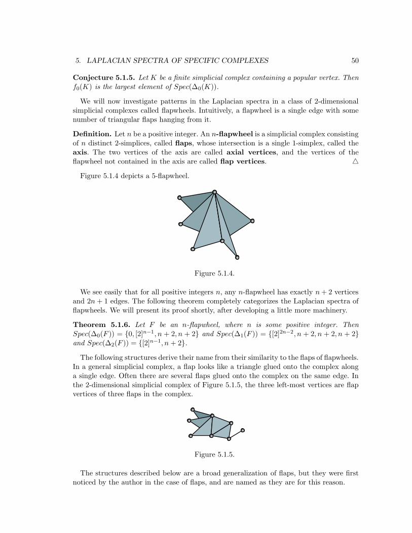
5. LAPLACIAN SPECTRA OF SPECIFIC COMPLEXES 50
Conjecture 5.1.5. Let K be a finite simplicial complex containing a popular vertex. Thenf0(K) is the largest element of Spec(∆0(K)).
We will now investigate patterns in the Laplacian spectra in a class of 2-dimensionalsimplicial complexes called flapwheels. Intuitively, a flapwheel is a single edge with somenumber of triangular flaps hanging from it.
Definition. Let n be a positive integer. An n-flapwheel is a simplicial complex consistingof n distinct 2-simplices, called flaps, whose intersection is a single 1-simplex, called theaxis. The two vertices of the axis are called axial vertices, and the vertices of theflapwheel not contained in the axis are called flap vertices. 4
Figure 5.1.4 depicts a 5-flapwheel.
Figure 5.1.4.
We see easily that for all positive integers n, any n-flapwheel has exactly n+ 2 verticesand 2n+ 1 edges. The following theorem completely categorizes the Laplacian spectra offlapwheels. We will present its proof shortly, after developing a little more machinery.
Theorem 5.1.6. Let F be an n-flapwheel, where n is some positive integer. ThenSpec(∆0(F )) = {0, [2]n−1, n + 2, n + 2} and Spec(∆1(F )) = {[2]2n−2, n + 2, n + 2, n + 2}and Spec(∆2(F )) = {[2]n−1, n+ 2}.
The following structures derive their name from their similarity to the flaps of flapwheels.In a general simplicial complex, a flap looks like a triangle glued onto the complex alonga single edge. Often there are several flaps glued onto the complex on the same edge. Inthe 2-dimensional simplicial complex of Figure 5.1.5, the three left-most vertices are flapvertices of three flaps in the complex.
Figure 5.1.5.
The structures described below are a broad generalization of flaps, but they were firstnoticed by the author in the case of flaps, and are named as they are for this reason.
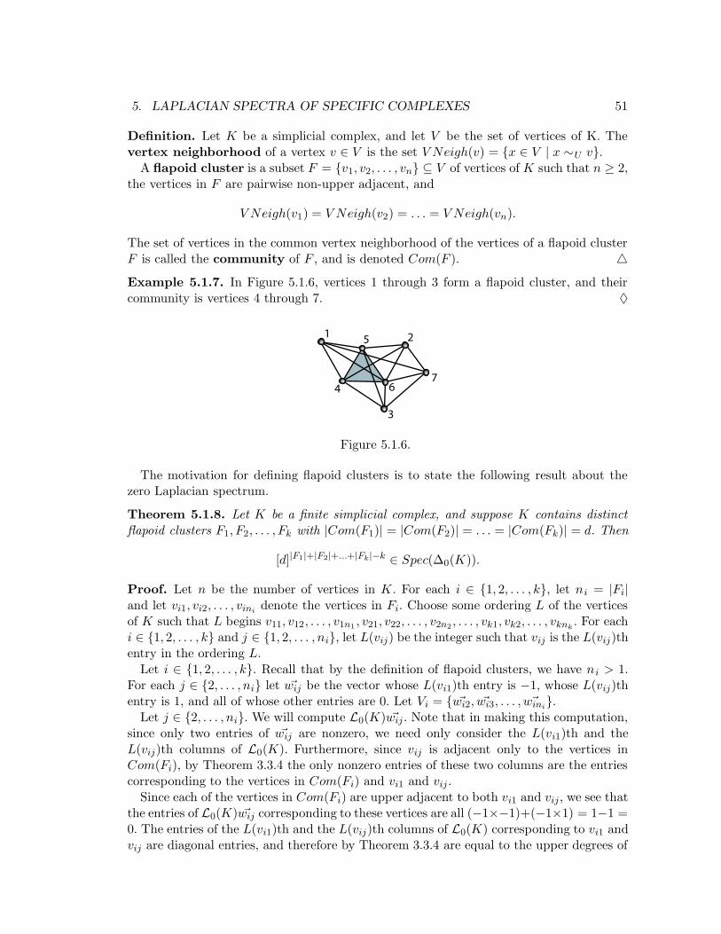
5. LAPLACIAN SPECTRA OF SPECIFIC COMPLEXES 51
Definition. Let K be a simplicial complex, and let V be the set of vertices of K. Thevertex neighborhood of a vertex v ∈ V is the set V Neigh(v) = {x ∈ V | x ∼U v}.
A flapoid cluster is a subset F = {v1, v2, . . . , vn} ⊆ V of vertices of K such that n ≥ 2,the vertices in F are pairwise non-upper adjacent, and
V Neigh(v1) = V Neigh(v2) = . . . = V Neigh(vn).
The set of vertices in the common vertex neighborhood of the vertices of a flapoid clusterF is called the community of F , and is denoted Com(F ). 4Example 5.1.7. In Figure 5.1.6, vertices 1 through 3 form a flapoid cluster, and theircommunity is vertices 4 through 7. ♦
1 2
3
4
5
67
Figure 5.1.6.
The motivation for defining flapoid clusters is to state the following result about thezero Laplacian spectrum.
Theorem 5.1.8. Let K be a finite simplicial complex, and suppose K contains distinctflapoid clusters F1, F2, . . . , Fk with |Com(F1)| = |Com(F2)| = . . . = |Com(Fk)| = d. Then
[d]|F1|+|F2|+...+|Fk|−k ∈ Spec(∆0(K)).
Proof. Let n be the number of vertices in K. For each i ∈ {1, 2, . . . , k}, let ni = |Fi|and let vi1, vi2, . . . , vini
denote the vertices in Fi. Choose some ordering L of the verticesof K such that L begins v11, v12, . . . , v1n1
, v21, v22, . . . , v2n2, . . . , vk1, vk2, . . . , vknk
. For eachi ∈ {1, 2, . . . , k} and j ∈ {1, 2, . . . , ni}, let L(vij) be the integer such that vij is the L(vij)thentry in the ordering L.
Let i ∈ {1, 2, . . . , k}. Recall that by the definition of flapoid clusters, we have ni > 1.For each j ∈ {2, . . . , ni} let ~wij be the vector whose L(vi1)th entry is −1, whose L(vij)thentry is 1, and all of whose other entries are 0. Let Vi = { ~wi2, ~wi3, . . . , ~wini
}.Let j ∈ {2, . . . , ni}. We will compute L0(K) ~wij . Note that in making this computation,
since only two entries of ~wij are nonzero, we need only consider the L(vi1)th and theL(vij)th columns of L0(K). Furthermore, since vij is adjacent only to the vertices inCom(Fi), by Theorem 3.3.4 the only nonzero entries of these two columns are the entriescorresponding to the vertices in Com(Fi) and vi1 and vij .
Since each of the vertices in Com(Fi) are upper adjacent to both vi1 and vij , we see thatthe entries of L0(K) ~wij corresponding to these vertices are all (−1×−1)+(−1×1) = 1−1 =0. The entries of the L(vi1)th and the L(vij)th columns of L0(K) corresponding to vi1 andvij are diagonal entries, and therefore by Theorem 3.3.4 are equal to the upper degrees of
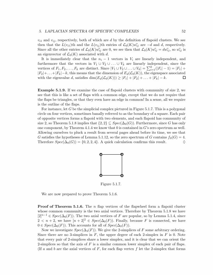
5. LAPLACIAN SPECTRA OF SPECIFIC COMPLEXES 52
vi1 and vij, respectively, both of which are d by the definition of flapoid clusters. We seethen that the L(vi1)th and the L(vij)th entries of L0(K) ~wij are −d and d, respectively.Since all the other entries of L0(K) ~wij are 0, we see then that L0(K) ~wij = d ~wij , so ~wij isan eigenvector of L0(K) associated with d.
It is immediately clear that the ni − 1 vectors in Vi are linearly independent, andfurthermore that the vectors in V1 ∪ V2 ∪ . . . ∪ Vk are linearly independent, since thevertices of F1, F2, . . . , Fk are distinct. Since |V1 ∪ V2 ∪ . . . ∪ Vk| =
∑ki=1(|Fi| − 1) = |F1| +
|F2|+. . .+|Fk|−k, this means that the dimension of Ed(L0(K)), the eigenspace associatedwith the eigenvalue d, satisfies dim(Ed(L0(K))) ≥ |F1| + |F2| + . . .+ |Fk| − k.
Example 5.1.9. If we examine the case of flapoid clusters with community of size 2, wesee that this is like a set of flaps with a common edge, except that we do not require thatthe flaps be triangles, or that they even have an edge in common! In a sense, all we requireis the outline of the flaps.
For instance, let G be the simplicial complex pictured in Figure 5.1.7. This is a polygonalcircle on four vertices, sometimes banally referred to as the boundary of a square. Each pairof opposite vertices forms a flapoid with two elements, and each flapoid has community ofsize 2, so Theorem 5.1.8 implies that {2, 2} ⊆ Spec(∆0(G)). Furthermore, since G has onlyone component, by Theorem 4.1.4 we know that 0 is contained inG’s zero spectrum as well.Allowing ourselves to pluck a result from several pages ahead before its time, we see thatG satisfies the hypotheses of Lemma 5.1.12, so the zero spectrum of G contains f0(G) = 4.Therefore Spec(∆0(G)) = {0, 2, 2, 4}. A quick calculation confirms this result. ♦
Figure 5.1.7.
We are now prepared to prove Theorem 5.1.6.
Proof of Theorem 5.1.6. The n flap vertices of the flapwheel form a flapoid clusterwhose common community is the two axial vertices. Therefore by Theorem 5.1.8 we have[2]n−1 ∈ Spec(∆0(F )). The two axial vertices of F are popular, so by Lemma 5.1.4, since2 < n + 2, we have [n + 2]2 ∈ Spec(∆0(F )). Finally, because F is connected, we have0 ∈ Spec(∆0(F )). This accounts for all of Spec(∆0(F )).
Now we investigate Spec(∆2(F )). We give the 2-simplices of F some arbitrary ordering.Since there are no 3-simplices in F , the upper degree of each 2-simplex in F is 0. Notethat every pair of 2-simplices share a lower simplex, and it is clear that we can orient the2-simplices so that the axis of F is a similar common lower simplex of each pair of flaps.(If a and b are the axial vertices of F , for each flap vertex f let the 2-simplex that forms
5. LAPLACIAN SPECTRA OF SPECIFIC COMPLEXES 53
this flap have the orientation 〈f, a, b〉.) By Theorem 3.3.4, we have
L2 =
3 1 . . . 11 3 . . . 1...
.... . .
...1 1 . . . 3
.
Again, let ~u denote the n-dimensional column vector whose components are all 1. Foreach i ∈ {1, 2, . . . , n − 1}, let ~vi denote the n-dimensional column vector whose coordi-nates are all 0 except that the last coordinate is −1 and the ith coordinate is 1. We willdemonstrate that {~v1, ~v2, . . . , ~vn−1, ~u} is a basis for C2 consisting of eigenvectors of L2.(Similarly to before, if n = 1, then we ignore ~v1, ~v2, . . . , ~vn−1. In what follows, note thatthe same arguments essentially hold if n = 1 and we have no such vectors ~v1, ~v2, . . . , ~vn−1.)
Suppose there are k1, k2, . . . , kn ∈ R such that
k1 ~v1 + k2 ~v2 + . . . + kn−1 ~vn−1 + kn~u = ~0.
By the definitions of these vectors, it follows that ki + kn = 0 for all i ∈ {1, 2, . . . , n− 1},and also that −k1 − k2 − . . . − kn−1 + kn = 0. From this first equation, it follows thatkn = −ki for all i ∈ {1, 2, . . . , n− 1}, so the second equation becomes (n− 1)kn + kn = 0,so nkn = 0. Since n 6= 0, this implies that kn = 0, so k1 = k2 = . . . = kn−1 = 0. Therefore{~v1, ~v2, . . . , ~vn−1, ~u} is linearly independent, and since this set contains n elements it mustbe a basis for C2.
Now, note that
L2~u =
3 1 . . . 11 3 . . . 1...
.... . .
...1 1 . . . 3
11...1
=
3 + (n− 1)3 + (n− 1)
...3 + (n− 1)
=
n+ 2n+ 2
...n+ 2
= (n+ 2)~u,
so ~u ∈ En+2(L2). Observe also that
L2~vi =
3 1 . . . 11 3 . . . 1...
.... . .
...1 1 . . . 3
0...010...0−1
=
1 − 1...
1 − 13 − 11 − 1
...1 − 11 − 3
=
0...020...0−2
= 2~vi
for all i ∈ {1, 2, . . . , n− 1}, where the middle coordinate in each column vector in betweenthe vertical dots is the ith coordinate,so ~vi ∈ E2(L2). Since {~v1, ~v2, . . . , ~vn−1, ~u} is a basisfor C2, it follows that Spec(∆2(F )) = {n+ 2, [2]n−1}.
The statement about Spec(∆1(F )) follows immediately from Corollary 4.1.9 and ourresults about Spec(∆0(F )) and Spec(∆2(F )).
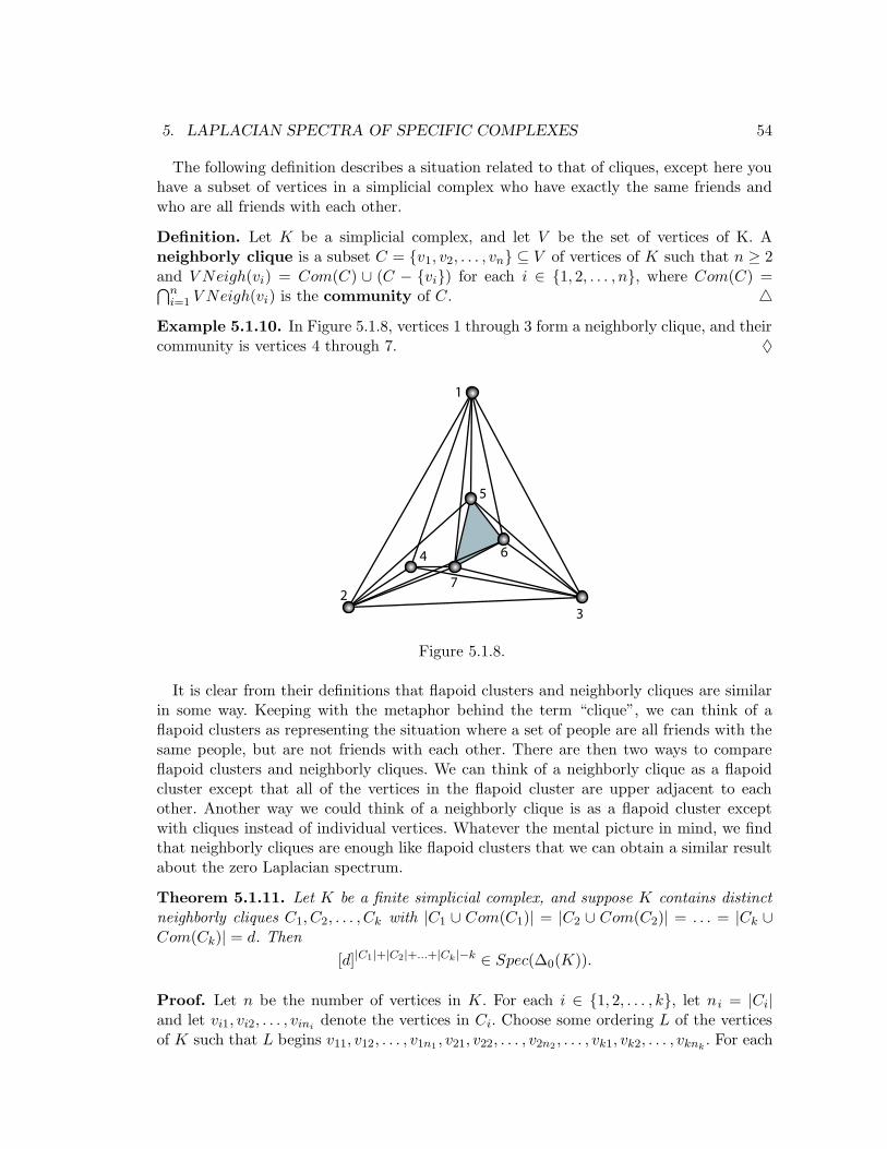
5. LAPLACIAN SPECTRA OF SPECIFIC COMPLEXES 54
The following definition describes a situation related to that of cliques, except here youhave a subset of vertices in a simplicial complex who have exactly the same friends andwho are all friends with each other.
Definition. Let K be a simplicial complex, and let V be the set of vertices of K. Aneighborly clique is a subset C = {v1, v2, . . . , vn} ⊆ V of vertices of K such that n ≥ 2and V Neigh(vi) = Com(C) ∪ (C − {vi}) for each i ∈ {1, 2, . . . , n}, where Com(C) =⋂n
i=1 V Neigh(vi) is the community of C. 4Example 5.1.10. In Figure 5.1.8, vertices 1 through 3 form a neighborly clique, and theircommunity is vertices 4 through 7. ♦
1
2
3
4
5
6
7
Figure 5.1.8.
It is clear from their definitions that flapoid clusters and neighborly cliques are similarin some way. Keeping with the metaphor behind the term “clique”, we can think of aflapoid clusters as representing the situation where a set of people are all friends with thesame people, but are not friends with each other. There are then two ways to compareflapoid clusters and neighborly cliques. We can think of a neighborly clique as a flapoidcluster except that all of the vertices in the flapoid cluster are upper adjacent to eachother. Another way we could think of a neighborly clique is as a flapoid cluster exceptwith cliques instead of individual vertices. Whatever the mental picture in mind, we findthat neighborly cliques are enough like flapoid clusters that we can obtain a similar resultabout the zero Laplacian spectrum.
Theorem 5.1.11. Let K be a finite simplicial complex, and suppose K contains distinctneighborly cliques C1, C2, . . . , Ck with |C1 ∪ Com(C1)| = |C2 ∪ Com(C2)| = . . . = |Ck ∪Com(Ck)| = d. Then
[d]|C1|+|C2|+...+|Ck|−k ∈ Spec(∆0(K)).
Proof. Let n be the number of vertices in K. For each i ∈ {1, 2, . . . , k}, let ni = |Ci|and let vi1, vi2, . . . , vini
denote the vertices in Ci. Choose some ordering L of the verticesof K such that L begins v11, v12, . . . , v1n1
, v21, v22, . . . , v2n2, . . . , vk1, vk2, . . . , vknk
. For each
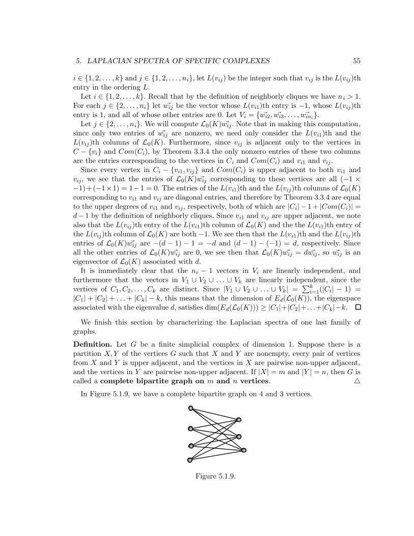
5. LAPLACIAN SPECTRA OF SPECIFIC COMPLEXES 55
i ∈ {1, 2, . . . , k} and j ∈ {1, 2, . . . , ni}, let L(vij) be the integer such that vij is the L(vij)thentry in the ordering L.
Let i ∈ {1, 2, . . . , k}. Recall that by the definition of neighborly cliques we have ni > 1.For each j ∈ {2, . . . , ni} let ~wij be the vector whose L(vi1)th entry is −1, whose L(vij)thentry is 1, and all of whose other entries are 0. Let Vi = { ~wi2, ~wi3, . . . , ~wini
}.Let j ∈ {2, . . . , ni}. We will compute L0(K) ~wij . Note that in making this computation,
since only two entries of ~wij are nonzero, we need only consider the L(vi1)th and theL(vij)th columns of L0(K). Furthermore, since vij is adjacent only to the vertices inC − {vi} and Com(Ci), by Theorem 3.3.4 the only nonzero entries of these two columnsare the entries corresponding to the vertices in Ci and Com(Ci) and vi1 and vij.
Since every vertex in Ci − {vi1, vij} and Com(Ci) is upper adjacent to both vi1 andvij , we see that the entries of L0(K) ~wij corresponding to these vertices are all (−1 ×−1)+(−1×1) = 1−1 = 0. The entries of the L(vi1)th and the L(vij)th columns of L0(K)corresponding to vi1 and vij are diagonal entries, and therefore by Theorem 3.3.4 are equalto the upper degrees of vi1 and vij, respectively, both of which are |Ci| − 1 + |Com(Ci)| =d− 1 by the definition of neighborly cliques. Since vi1 and vij are upper adjacent, we notealso that the L(vij)th entry of the L(vi1)th column of L0(K) and the the L(vi1)th entry ofthe L(vij)th column of L0(K) are both −1. We see then that the L(vi1)th and the L(vij)thentries of L0(K) ~wij are −(d − 1) − 1 = −d and (d − 1) − (−1) = d, respectively. Sinceall the other entries of L0(K) ~wij are 0, we see then that L0(K) ~wij = d ~wij , so ~wij is aneigenvector of L0(K) associated with d.
It is immediately clear that the ni − 1 vectors in Vi are linearly independent, andfurthermore that the vectors in V1 ∪ V2 ∪ . . . ∪ Vk are linearly independent, since thevertices of C1, C2, . . . , Ck are distinct. Since |V1 ∪ V2 ∪ . . . ∪ Vk| =
∑ki=1(|Ci| − 1) =
|C1| + |C2| + . . . + |Ck| − k, this means that the dimension of Ed(L0(K)), the eigenspaceassociated with the eigenvalue d, satisfies dim(Ed(L0(K))) ≥ |C1|+|C2|+. . .+|Ck|−k.
We finish this section by characterizing the Laplacian spectra of one last family ofgraphs.
Definition. Let G be a finite simplicial complex of dimension 1. Suppose there is apartition X,Y of the vertices G such that X and Y are nonempty, every pair of verticesfrom X and Y is upper adjacent, and the vertices in X are pairwise non-upper adjacent,and the vertices in Y are pairwise non-upper adjacent. If |X| = m and |Y | = n, then G iscalled a complete bipartite graph on m and n vertices. 4
In Figure 5.1.9, we have a complete bipartite graph on 4 and 3 vertices.
Figure 5.1.9.
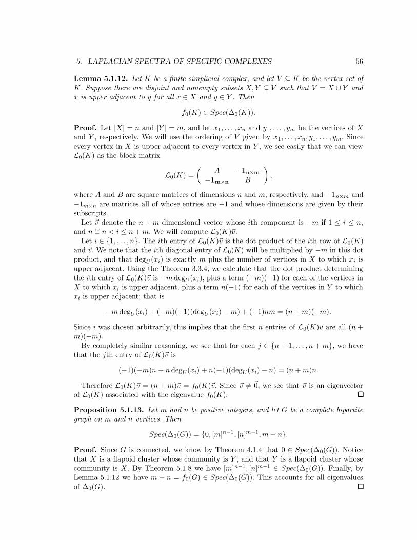
5. LAPLACIAN SPECTRA OF SPECIFIC COMPLEXES 56
Lemma 5.1.12. Let K be a finite simplicial complex, and let V ⊆ K be the vertex set ofK. Suppose there are disjoint and nonempty subsets X,Y ⊆ V such that V = X ∪ Y andx is upper adjacent to y for all x ∈ X and y ∈ Y . Then
f0(K) ∈ Spec(∆0(K)).
Proof. Let |X| = n and |Y | = m, and let x1, . . . , xn and y1, . . . , ym be the vertices of Xand Y , respectively. We will use the ordering of V given by x1, . . . , xn, y1, . . . , ym. Sinceevery vertex in X is upper adjacent to every vertex in Y , we see easily that we can viewL0(K) as the block matrix
L0(K) =
(A −1n×m
−1m×n B
),
where A and B are square matrices of dimensions n and m, respectively, and −1n×m and−1m×n are matrices all of whose entries are −1 and whose dimensions are given by theirsubscripts.
Let ~v denote the n + m dimensional vector whose ith component is −m if 1 ≤ i ≤ n,and n if n < i ≤ n+m. We will compute L0(K)~v.
Let i ∈ {1, . . . , n}. The ith entry of L0(K)~v is the dot product of the ith row of L0(K)and ~v. We note that the ith diagonal entry of L0(K) will be multiplied by −m in this dotproduct, and that degU (xi) is exactly m plus the number of vertices in X to which xi isupper adjacent. Using the Theorem 3.3.4, we calculate that the dot product determiningthe ith entry of L0(K)~v is −mdegU (xi), plus a term (−m)(−1) for each of the vertices inX to which xi is upper adjacent, plus a term n(−1) for each of the vertices in Y to whichxi is upper adjacent; that is
−mdegU (xi) + (−m)(−1)(degU (xi) −m) + (−1)nm = (n+m)(−m).
Since i was chosen arbitrarily, this implies that the first n entries of L0(K)~v are all (n+m)(−m).
By completely similar reasoning, we see that for each j ∈ {n + 1, . . . , n+m}, we havethat the jth entry of L0(K)~v is
(−1)(−m)n+ ndegU (xi) + n(−1)(degU (xi) − n) = (n+m)n.
Therefore L0(K)~v = (n +m)~v = f0(K)~v. Since ~v 6= ~0, we see that ~v is an eigenvectorof L0(K) associated with the eigenvalue f0(K).
Proposition 5.1.13. Let m and n be positive integers, and let G be a complete bipartitegraph on m and n vertices. Then
Spec(∆0(G)) = {0, [m]n−1, [n]m−1,m+ n}.
Proof. Since G is connected, we know by Theorem 4.1.4 that 0 ∈ Spec(∆0(G)). Noticethat X is a flapoid cluster whose community is Y , and that Y is a flapoid cluster whosecommunity is X. By Theorem 5.1.8 we have [m]n−1, [n]m−1 ∈ Spec(∆0(G)). Finally, byLemma 5.1.12 we have m + n = f0(G) ∈ Spec(∆0(G)). This accounts for all eigenvaluesof ∆0(G).
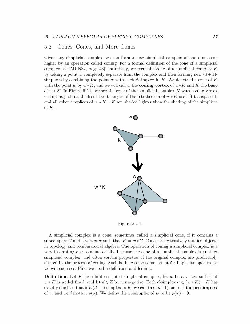
5. LAPLACIAN SPECTRA OF SPECIFIC COMPLEXES 57
5.2 Cones, Cones, and More Cones
Given any simplicial complex, we can form a new simplicial complex of one dimensionhigher by an operation called coning. For a formal definition of the cone of a simplicialcomplex see [MUN84, page 43]. Intuitively, we form the cone of a simplicial complex K
by taking a point w completely separate from the complex and then forming new (d+ 1)-simplices by combining the point w with each d-simplex in K. We denote the cone of Kwith the point w by w∗K, and we will call w the coning vertex of w∗K and K the baseof w ∗K. In Figure 5.2.1, we see the cone of the simplicial complex K with coning vertexw. In this picture, the front two triangles of the tetrahedron of w ∗K are left transparent,and all other simplices of w ∗K −K are shaded lighter than the shading of the simplicesof K.
K
w
w
w * K
Figure 5.2.1.
A simplicial complex is a cone, sometimes called a simplicial cone, if it contains asubcomplex G and a vertex w such that K = w ∗G. Cones are extensively studied objectsin topology and combinatorial algebra. The operation of coning a simplicial complex is avery interesting one combinatorially, because the cone of a simplicial complex is anothersimplicial complex, and often certain properties of the original complex are predictablyaltered by the process of coning. Such is the case to some extent for Laplacian spectra, aswe will soon see. First we need a definition and lemma.
Definition. Let K be a finite oriented simplicial complex, let w be a vertex such thatw ∗K is well-defined, and let d ∈ Z be nonnegative. Each d-simplex σ ∈ (w ∗K) −K hasexactly one face that is a (d−1)-simplex in K; we call this (d−1)-simplex the presimplexof σ, and we denote it p(σ). We define the presimplex of w to be p(w) = ∅.
5. LAPLACIAN SPECTRA OF SPECIFIC COMPLEXES 58
Let σ ∈ (w ∗K) −K be a d-simplex. The orientation of p(σ) in K can be representedby a list of its vertices [v1 . . . vd]. The standard orientation of σ induced by p(σ) isthe orientation given by
(−1)d[v1 . . . vd, w].
We say that w ∗K has the standard orientation induced by K if every simplex in Khas the same orientation in both K and w ∗K, and if every simplex in (w ∗K) −K hasthe standard orientation induced by its presimplex. 4Lemma 5.2.1. Let K be a finite oriented simplicial complex, let w be a vertex such thatw ∗K is well-defined, let w ∗K have the standard orientation induced by K, and let d ∈ Z
be nonnegative.
(1) For all distinct d-simplices σ1, σ2 ∈ (w ∗ K) −K, we have that σ1 and σ2 are up-per adjacent in w ∗ K iff p(σ1) and p(σ2) are upper adjacent in K. If σ1, σ2 andp(σ1), p(σ2) are upper adjacent, then σ1 and σ2 are similarly oriented iff p(σ1) andp(σ2) are similarly oriented.
(2) For all d-simplices σ ∈ K and σ′ ∈ (w ∗K) −K, we have that σ and σ′ are upperadjacent in w ∗ K iff the coefficient of p(σ ′) in ∂̃d(σ) is nonzero. If σ and σ′ areupper adjacent in w ∗K, then they are similarly or dissimilarly oriented in w ∗K iffthe coefficient of p(σ′) in ∂̃d(σ) is −1, or +1, respectively.
Proof. (1) Let σ1, σ2 ∈ (w ∗ K) − K be distinct d-simplices. Suppose p(σ1) and p(σ2)are upper adjacent. Then there is a d-simplex ζ ∈ K containing both p(σ1) and p(σ2) asfaces. Then w ∗ ω is a (d + 1)-simplex in w ∗K, and it must contain w ∗ p(σ1) = σ1 andw∗p(σ2) = σ2 as faces, so σ1 and σ2 are upper adjacent. Now suppose σ1 and σ2 are upperadjacent. Then there is a (d+1)-simplex τ ∈ w ∗K that contains σ1 and σ2 as faces. Notealso that τ contains w, so τ ∈ (w ∗K) −K. Then p(τ) is a d-simplex in K, and we seethat p(τ) contains both p(σ1) and p(σ2) as faces, so p(σ1) and p(σ2) are upper adjacent.
Therefore p(σ1) and p(σ2) are upper adjacent iff σ1 and σ2 are upper adjacent. Now wemust show that the similarities and dissimilarities match.
Suppose each of p(σ1), p(σ2) and σ1, σ2 are upper adjacent. By Lemma 3.4.4, we knowthat each pair p(σ1), p(σ2) and σ1, σ2 are similarly oriented with respect to their commonupper simplex iff the pair share a dissimilar reduced common lower simplex. We will showthat p(σ1) and p(σ2) share a similar reduced common lower simplex iff σ1 and σ2 share asimilar reduced common lower simplex, which will therefore suffice to complete our proofof part (1).
Let
p(σ1) = s1[v1v2 . . . vd−1x] and p(σ2) = s1[v1v2 . . . vd−1y],
where s1 and s2 are each ±1, depending on orientations. By the definition of standardinduced orientation we have that
σ1 = (−1)ds1[v1v2 . . . vd−1xw] and σ2 = (−1)ds1[v1v2 . . . vd−1yw].
The common reduced lower simplex of p(σ1) and p(σ1) is η = ±[v1v2 . . . vd−1], withthe sign depending on the orientation of η. Since the coefficients of η in ∂̃d−1(p(σ1))
5. LAPLACIAN SPECTRA OF SPECIFIC COMPLEXES 59
and ∂̃d−1(p(σ2)) are ±(−1)d−1s1 and ±(−1)d−1s2, respectively, we see that η is a similarreduced common lower simplex of p(σ1) and p(σ1) iff s1 = s2. The reduced common lowersimplex of σ1 and σ2 is η′ = ±[v1v2 . . . vd−1w], with the sign depending on the orientationof η′. Since the coefficients of η′ in ∂̃d(σ1) and ∂̃d(σ2) are ±(−1)d−1(−1)ds1 = ∓s1 and±(−1)d−1(−1)ds2 = ∓s2, we see that η′ is a similar reduced common lower simplex ofσ1 and σ2 iff s1 = s2. Therefore p(σ1) and p(σ2) share a similar reduced common lowersimplex iff σ1 and σ2 share a similar reduced common lower simplex.(2) Let σ ∈ K and σ′ ∈ (w ∗ K) −K be d-simplices. Suppose the coefficient of p(σ ′) in∂̃d(σ) is nonzero, meaning that p(σ′) is a face of σ. Then w ∗ σ is a (d + 1)-simplex inw ∗K that contains both σ and w ∗ p(σ′) = σ′ as faces, so σ and σ′ are upper adjacentin w ∗K. Suppose σ and σ′ are upper adjacent in w ∗K. Then σ and σ ′ must be loweradjacent in w ∗K, and there must be some (d − 1)-simplex that is a face of both σ andσ′. This (d − 1)-simplex must be in K and must also be a face of σ ′, so it must be p(σ′).Since p(σ′) is a proper face of σ, this presimplex must be contained in ∂̃d(σ).
Now we must show that the similarities match up. Suppose σ and σ ′ are upper adjacent.Then they are reduced lower adjacent with reduced common lower simplex p(σ ′). Letp(σ′) = [v1v2 . . . vd]. Then σ′ = (−1)d[v1v2 . . . vdw]. Then the coefficient of p(σ′) in ∂̃d(σ
′) is(−1)d(−1)d = +1. Since p(σ′) is the common lower simplex of σ and σ ′, using Lemma 3.4.4this implies that σ and σ′ are upper adjacent in w∗K and similarly, or dissimilarly oriented,iff they are reduced lower adjacent in w ∗K with dissimilar, or similar, reduced commonlower simplex iff the coefficient of p(σ ′) in ∂̃d(σ) is −1, or +1, respectively.
Now we are prepared to prove a very important result about cones of simplicial com-plexes. This theorem was first proved in [DURE, Corollary 4.11], where it is actually acorollary of a much stronger and more general result, but the proof given here is entirelyour own, and surprisingly is seen to rest largely on the Reduced Laplacian Matrix Theo-rem, Theorem 3.4.8. We state this result in our own notation, which looks rather differentfrom the original statement of this result. Recall the definitions of multiset sum and scaledmultiset from the definitions at the beginning of Section 2.2.
Theorem 5.2.2. Let K be a finite simplicial complex, let w be a vertex such that w ∗Kis well-defined, and let d ∈ Z be nonnegative. Then
SpecNZ(∆̃UPd (w ∗K)) = {[1]fd(K)} +M Spec(∆̃d(K)).
Proof. Let fd(K) = m and fd−1(K) = n. Let σ1, . . . , σm ∈ K and σm+1, . . . , σm+n ∈(w ∗K) −K be all the d-simplices of w ∗K, and for all i ∈ {1, . . . , n} let ηi = p(σm+i).Note that since each (d− 1)-simplex in K corresponds to a d-simplex in (w ∗K)−K, theset {η1, . . . , ηn} represents all the (d − 1)-simplices of K. This proof proceeds in severalsteps.STEP (1): First we will demonstrate that
L̃UPd (w ∗K) =
(L̃UP
d (K) + Im B̃Td (K)
B̃d(K) L̃UPd−1(K)
),
where Im is the m×m identity matrix.
5. LAPLACIAN SPECTRA OF SPECIFIC COMPLEXES 60
Let i, j ∈ {1, . . . ,m}. Suppose i = j. Then by the Reduced Laplacian Matrix Theorem,Theorem 3.4.8, the ith diagonal entry of L̃UP
d (w ∗K) is the upper degree of σi in w ∗K.Note that the upper degree of σi in w ∗K is precisely one more that its upper degree inK, because there is only one (d + 1)-simplex in (w ∗ K) − K that contains σi, namelyw ∗ σi. Suppose i 6= j. Then by the Reduced Laplacian Matrix Theorem, the ijth entry ofL̃UP
d (w ∗K) is 0 if σi and σj are not upper adjacent in w ∗K, and +1 or −1 if they areupper adjacent and similarly or dissimilarly oriented, respectively. Note that there cannotbe a (d + 1)-simplex in w ∗ K containing both σi and σj that is not in K, so these twod-simplices are upper adjacent in w ∗ K iff they are upper adjacent in K. Also, by thedefinition of the induced standard orientation of w ∗K, the orientations of σi and σj in K
and w ∗K are identical. Therefore, we see that the ijth component of L̃UPd (w ∗K) is the
same as the ijth component of L̃UPd (K). It follows then that the m×m upper left block
of L̃UPd (w ∗ K) is identical to L̃UP
d (K) + Im, where the latter matrix is calculated withrespect to the ordered basis {σ1, . . . , σm}.
Let i, j ∈ {m + 1, . . . ,m + n}. Suppose i = j. Then by the Reduced Laplacian MatrixTheorem the ith diagonal entry of L̃UP
d (w ∗K) is the upper degree of σi in w ∗K. It is notdifficult to see that the number of (d+ 1)-simplices in w ∗K containing σi ∈ (w ∗K)−K
as a face is the same as the number of d-simplices in K containing p(σi) = ηi−m. Thereforethe upper degree of σi in w ∗K is equal to the upper degree of ηi−m in K. Now, supposei 6= j. By Lemma 5.2.1(1), we know that σi and σj are upper adjacent iff p(σi) = ηi−m andp(σj) = ηj−m are upper adjacent K, and that if each pair of simplices is upper adjacentthen the pairs are similarly, or dissimilarly, oriented simulataneously. Therefore, we seethat the n× n lower right block of L̃UP
d (w ∗K) is identical to L̃UPd−1(K), where the latter
matrix is calculated with respect to the ordered basis {η1, . . . , ηn}.Let i ∈ {m + 1, . . . ,m + n} and j ∈ {1, . . . m}. By the Reduced Laplacian Matrix
Theorem, Theorem 3.4.8(2), and the definition of the matrix representation of ∂̃d(K), theijth entry of L̃UP
d (w ∗ K) is 0 if σi and σj are not upper adjacent in w ∗ K; and +1 or−1 if they are upper adjacent and similarly or dissimilarly oriented, respectively, which isthe case iff the coefficient of p(σi) = ηi−m in ∂̃d(σj) is −1, or +1, respectively, which is
the case iff the ijth entry of B̃d(K) is −1 or +1, respectively, where B̃d(K) is the matrixof ∂̃d(K) with respect to the ordered bases {σ1, . . . , σm} and {η1, . . . , ηn} for the d-chainsand (d − 1)-chains of K, respectively. Therefore, it follows that the lower left block ofL̃UP
d (w ∗K) is identical to B̃d(K). Since L̃UPd (w ∗K) is a symmetric matrix, this implies
that the upper right block of L̃UPd (w ∗K) is identical to B̃T
d (K).STEP (2): (In this part, we will be doing many calculations with block matrices and blockvectors. The reader should verify that the dimensions of appropriate blocks match upthroughout our calculations.) Let
X =
(L̃UP
d + Im −B̃Td
−B̃d L̃UPd−1
)=
(B̃d+1B̃T
d+1 + Im −B̃Td
−B̃d B̃dB̃Td
)
and
Y =
(L̃d + Im 0
0 0
)=
(B̃d+1B̃T
d+1 + B̃Td B̃d + Im 0
0 0
).
5. LAPLACIAN SPECTRA OF SPECIFIC COMPLEXES 61
(For simplicity, in this step we will omit the arguments from our matrix symbols, andassume that every matrix is with respect to K.) We will demonstrate that Spec(X) =Spec(Y ).
Let
P =
(Im B̃T
d
−B̃d In
).
Keeping in mind that ∂̃i∂̃i+1 is the zero transformation, and hence B̃iB̃i+1 is the zeromatrix, for all nonnegative integers i, the reader should verify that
PX = Y P =
(B̃d+1B̃T
d+1 + B̃Td B̃d + Im B̃T
d B̃dB̃Td + B̃T
d
0 0
).
Now if we can show that P is invertible, then it follows that X = P −1Y P . From [FIS97,Exercise 12(a), page 249], it would then follow that Spec(X) = Spec(Y ). We prove thatP is invertible indirectly. Let
Q =
(Im −B̃T
d
B̃d In
).
Then
PQ =
(Im B̃T
d
−B̃d In
)(Im −B̃T
d
B̃d In
)=
(B̃T
d B̃d + Im 0
0 B̃dB̃Td + In
)
=
(B̃T
d B̃d 0
0 B̃dB̃Td
)+ Im+n =
(B̃T
d 0
0 B̃d
)(B̃d 0
0 B̃Td
)+ Im+n
=
(B̃T
d 0
0 B̃d
)(B̃T
d 0
0 B̃d
)T
+ Im+n.
Label the first term in the last equality A. By Lemma 2.2.8 we know that A represents apositive semidefinite linear operator, so by Lemma 2.2.7 the eigenvalues of A are nonnega-tive. Note also that adding Im+n to A has the effect of adding 1 to each eigenvalue, so thatSpec(A+ Im+n) = {1, 1, . . . , 1}+M Spec(A). Therefore the eigenvalues of PQ = A+ Im+n
are strictly positive. This means that 0 is not an eigenvalue of PQ, which means that thenullspace of the operator represented by PQ is trivial, which implies that PQ is invertible.Then
det(P ) det(Q) = det(PQ) 6= 0,
so det(P ) 6= 0, so P is invertible.STEP (3): Putting Steps (1) and (2) together, we have proven that
Spec(∆UPd (w ∗K)) = Spec(X) = Spec(Y ) = {[0]n} ∪M
({[1]m} +M Spec(∆̃d(K))
).
Since the elements of {[1]m} +M Spec(∆̃d(K)) are strictly positive, this implies that
SpecNZ(∆̃UPd (w ∗K)) = {[1]fd(K)} +M Spec(∆̃d(K)).
5. LAPLACIAN SPECTRA OF SPECIFIC COMPLEXES 62
From Lemma 4.1.7 and Theorem 5.2.2 we immediately have the following corollary.
Corollary 5.2.3. Let K be a finite simplicial complex, let w be a vertex such that w ∗Kis well-defined, and let d ∈ Z be nonnegative. Then
SpecNZ(∆̃d(w ∗K)) = {[1]fd(K)+fd−1(K)} +M
(Spec(∆̃d(K)) ∪M Spec(∆̃d−1(K))
).
In the case of 2-dimensional cones, Theorem 5.2.2 leads to some truly fascinating results.
Theorem 5.2.4. Let K be a finite simplicial cone of dimension less than or equal to 2,with base G ⊆ K. Then
SpecNZ(∆0(K)) =
[{[1]f0(G)−1}+M
(SpecNZ(∆0(G))
)f0(G)−1
]∪M {f0(G) + 1} (5.2.1)
andSpec(∆2(K)) = {[1]f1(G)}+M
(SpecNZ(∆0(G))
)f1(G)
. (5.2.2)
Proof. Let v be a vertex of K such that K = v ∗ G. Note that f1(G) = f2(K) andf0(G) + 1 = f0(K).
We know that ∆0(K) = ∆UP0 (K) = ∆̃UP
0 (K), so by Theorem 5.2.2 and Lemma 4.1.7we have
SpecNZ(∆0(K)) = {[1]f0(G)}+MSpec(∆̃0(G))
= {[1]f0(G)}+M
(SpecNZ(∆̃DN
0 (G)) ∪M SpecNZ(∆̃UP0 (G))
)f0(G)
.
It follows from Lemma 2.2.9 that SpecNZ(∆̃DN0 (G)) = SpecNZ(Uf0(G)) = {f0(G)}, and
as before we see that SpecNZ(∆̃UP0 (G)) = SpecNZ(∆0(G)). Therefore
SpecNZ(∆0(K)) = {[1]f0(G)}+M
(SpecNZ(∆0(G)) ∪M {f0(G)}
)f0(G)
=
[{[1]f0(G)−1}+M
(SpecNZ(∆0(G))
)f0(G)−1
]∪M {f0(G) + 1}.
Since K is at most 2-dimensional, we know ∆2(K) = ∆DN2 (K), and also that
SpecNZ(∆DN2 (K)) = SpecNZ(∆UP
1 (K)) = SpecNZ(∆̃UP1 (K)). Therefore by Theo-
rem 5.2.2 it follows that
SpecNZ(∆2(K)) = {[1]f1(G)}+MSpec(∆̃1(G))
= {[1]f1(G)}+M
(SpecNZ(∆̃DN
1 (G)) ∪M SpecNZ(∆̃UP1 (G))
)f1(G)
.
Lemma 4.1.8 and some simplification yield that SpecNZ(∆̃DN1 (G)) = SpecNZ(∆̃UP
0 (G)) =
SpecNZ(∆0(G)) and SpecNZ(∆̃UP1 (G)) = SpecNZ(∆̃DN
2 (G)) = SpecNZ(∆DN2 (G)) =
SpecNZ(∆2(G)). Furthermore, since K is at most 2-dimensional it must be the case that Gis at most 1-dimensional, so ∆2(G) is a zero matrix and SpecNZ(∆2(G)) = ∅. Finally, The-orem 4.1.4 implies that H2(K; R) ∼= N(∆2(K)), and since H2(K; R) is zero dimensional
5. LAPLACIAN SPECTRA OF SPECIFIC COMPLEXES 63
since K is a cone, we know 0 is not in Spec(∆2(K)), so SpecNZ(∆2(K)) = Spec(∆2(K)).Therefore
Spec(∆2(K)) = {[1]f1(G)}+M
(SpecNZ(∆0(G))
)f1(G)
.
Theorem 5.2.5. Let K be a finite simplicial cone of dimension less than or equal to 2.
(i) If f0(K) ≥ f2(K) + 2, then
Spec(∆0(K)) = Spec(∆2(K)) ∪M {0, [1]f0(K)−f2(K)−2, f0(K)}.
(ii) If f0(K) < f2(K) + 2, then
Spec(∆0(K)) ∪M {[1]f2(K)−f0(K)+2} = Spec(∆2(K)) ∪M {0, f0(K)}.
Proof. Let K = v ∗G. Note that f0(G) + 1 = f0(K) and f1(G) = f2(K).For part (i), suppose f0(K) ≥ f2(K) + 2. Then f0(K) − 2 ≥ f2(K). Then from Equa-
tions 5.2.1 and 5.2.2 of Theorem 5.2.4, and recalling that f0(G) + 1 = f0(K) andf1(G) = f2(K), we have
SpecNZ(∆0(K)) =
[{[1]f0(K)−2}+M
(SpecNZ(∆0(G))
)f0(K)−2
]∪M {f0(K)}
=
[{[1]f2(K)}+M
(SpecNZ(∆0(G))
)f2(K)
]
∪M
[{[1]f0(K)−f2(K)−2}+M{[0]f0(K)−f2(K)−2}
]∪M {f0(K)}
= Spec(∆2(K)) ∪M {[1]f0(K)−f2(K)−2, f0(K)}.
The last expression in this chain of equalities has exactly f2(K)+f0(K)−f2(K)−2+1 =f0(K) − 1 elements. Hence we conclude that
Spec(∆0(K)) = Spec(∆2(K)) ∪M {0, [1]f0(K)−f2(K)−2, f0(K)}.
For part (ii), suppose f0(K) < f2(K) + 2. Then f2(K) > f0(K) − 2. Also, from Theo-rem 4.1.4 we know 0 ∈ Spec(∆0(G)), so SpecNZ(∆0(G)) has no more than f0(G) − 1 =f0(K)−2 < f2(K) elements, so at least f2(K)−(f0(K)−2) = f2(K)−f0(K)+2 elements
of(SpecNZ(∆0(G))
)f2(K)
are 0. Then from Equations 5.2.1 and 5.2.2 of Theorem 5.2.4
we have
Spec(∆2(K)) = {[1]f2(K)}+M
(SpecNZ(∆0(G))
)f2(K)
=
[{[1]f0(K)−2}+M
(SpecNZ(∆0(G))
)
f0(K)−2
]
∪M
[{[1]f2(K)−f0(K)+2}+M{[0]f2(K)−f0(K)+2}
]
= [SpecNZ(∆0(K)) − {f0(K)}] ∪M {[1]f2(K)−f0(K)+2}.
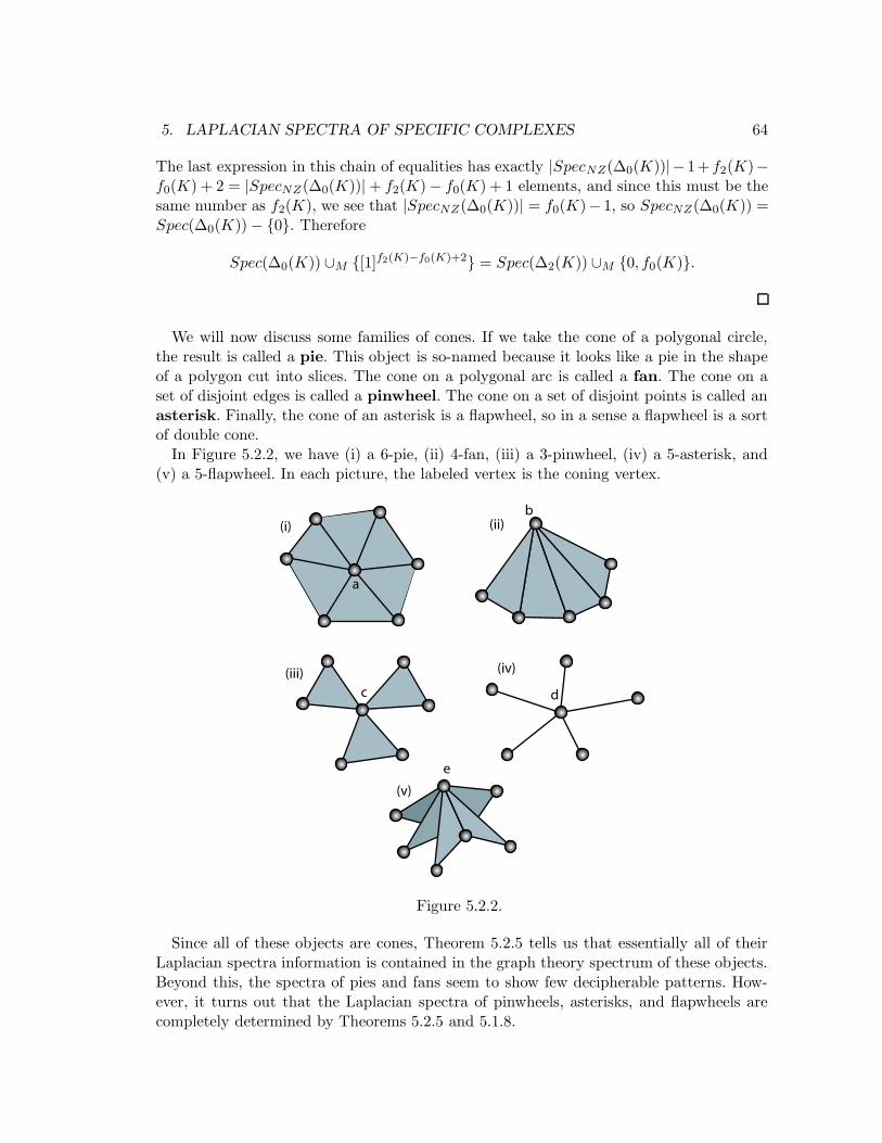
5. LAPLACIAN SPECTRA OF SPECIFIC COMPLEXES 64
The last expression in this chain of equalities has exactly |SpecNZ(∆0(K))|− 1+ f2(K)−f0(K) + 2 = |SpecNZ(∆0(K))| + f2(K) − f0(K) + 1 elements, and since this must be thesame number as f2(K), we see that |SpecNZ(∆0(K))| = f0(K)− 1, so SpecNZ(∆0(K)) =Spec(∆0(K)) − {0}. Therefore
Spec(∆0(K)) ∪M {[1]f2(K)−f0(K)+2} = Spec(∆2(K)) ∪M {0, f0(K)}.
We will now discuss some families of cones. If we take the cone of a polygonal circle,the result is called a pie. This object is so-named because it looks like a pie in the shapeof a polygon cut into slices. The cone on a polygonal arc is called a fan. The cone on aset of disjoint edges is called a pinwheel. The cone on a set of disjoint points is called anasterisk. Finally, the cone of an asterisk is a flapwheel, so in a sense a flapwheel is a sortof double cone.
In Figure 5.2.2, we have (i) a 6-pie, (ii) 4-fan, (iii) a 3-pinwheel, (iv) a 5-asterisk, and(v) a 5-flapwheel. In each picture, the labeled vertex is the coning vertex.
a
b
c d
e
(i) (ii)
(iii) (iv)
(v)
Figure 5.2.2.
Since all of these objects are cones, Theorem 5.2.5 tells us that essentially all of theirLaplacian spectra information is contained in the graph theory spectrum of these objects.Beyond this, the spectra of pies and fans seem to show few decipherable patterns. How-ever, it turns out that the Laplacian spectra of pinwheels, asterisks, and flapwheels arecompletely determined by Theorems 5.2.5 and 5.1.8.
5. LAPLACIAN SPECTRA OF SPECIFIC COMPLEXES 65
Lemma 5.2.6. Let P be a pinwheel, and let f2(P ) = n > 0. Then Spec(∆0(P )) ={0, [1]n−1, [3]n, 2n + 1} and Spec(∆1(P )) = {[1]n−1, [3]2n, 2n + 1} and Spec(∆2(P )) ={[3]n}.
Proof. Note first that f0(P ) = 2f2(P )+1 = 2n+1 and f1(P ) = 3n. It is easy to see thatfor all positive integers m the inequality 2m ≥ m + 1 holds. That P is nontrivial meansthat n ≥ 1, so f0(P ) = 2n+ 1 ≥ n+ 2 = f2(P ) + 2. Hence by Theorem 5.2.5 we have
Spec(∆0(P )) = Spec(∆2(P )) ∪M {0, [1]n−1, 2n+ 1}.None of the 2-simplices of P are upper adjacent to each other, so by Theorem 3.3.4 wesee that L2(P ) = 3In, where In is the n × n identity matrix, so Spec(∆2(P )) = {[3]n}.Therefore Spec(∆0(P )) = {0, [1]n−1, [3]n, 2n+ 1}.
The statement about Spec(∆1(P )) follows from Corollary 4.1.9, and the fact thatf1(P ) = 3n.
Lemma 5.2.7. Let A be an asterisk, and let f0(A) = n > 0. Then Spec(∆0(A)) ={0, [1]n−2, n} and Spec(∆1(A)) = {[1]n−2, n}.
Proof. Since A contains no 2-simplices, by Theorem 5.2.5 we have Spec(∆0(A)) =Spec(∆2(P ))∪M {0, [1]n−2, n} = {0, [1]n−2, n}. Since A is 1-dimensional, we have ∆1(A) =∆DN
1 (A). Since ∆0(A) = ∆UP0 (A) and A has one fewer edges than vertices, we see by
Lemma 4.1.8 that Spec(∆1(A)) = SpecNZ(∆0(A)) = {[1]n−2, n}.
Viewing flapwheels as simplicial cones, we now have another proof of Theorem 5.1.6.
Alternate proof of Theorem 5.1.6. As a reminder, we have a flapwheel F with n > 1flaps. As noted above, we see that F is combinatorically equivalent to a cone on an asteriskA with n+1 vertices. By Equation 5.2.1 from the proof of Theorem 5.2.4, and Lemma 5.2.7above, we have
SpecNZ(∆0(F )) =
[{[1]f0(F )−2}+M
(SpecNZ(∆0(A))
)f0(F )−2
]∪M {f0(F )}
=[{[1]n}+M
(SpecNZ(∆0(A))
)n
]∪M {n+ 2}
=[{[1]n}+M
({[1]n−1, n+ 1}
)n
]∪M {n+ 2}
=[{[1]n}+M{[1]n−1, n+ 1}
]∪M {n+ 2}
= {[2]n−1, n+ 2} ∪M {n+ 2}= {[2]n−1, n+ 2, n+ 2}.
By counting, we see that we are short by a single eigenvalue to get from SpecNZ(∆0(F ))to Spec(∆0(F )), so Spec(∆0(F )) = {0, [2]n−1, n+ 2, n+ 2}.
Now, by Equation 5.2.2 from Theorem 5.2.4, and Proposition 5.2.7 above, we have
Spec(∆2(F )) = {[1]f2(F )}+M
(SpecNZ(∆0(A))
)f2(F )
= {[1]n}+M
({[1]n−1, n+ 1}
)
n
= {[2]n−1, n+ 2}.
5. LAPLACIAN SPECTRA OF SPECIFIC COMPLEXES 66
As mentioned at the end of the original proof of Theorem 5.1.6, the result aboutSpec(∆1(F )) follows directly from our results about Spec(∆0(F )) and Spec(∆2(F )).
Finally, since a simplex is itself a simplicial complex, we are able to use our results aboutcones to prove the following tidy fact about the Laplacian spectra of simplices.
Proposition 5.2.8. Let n ∈ Z be nonnegative, and let σn denote the n-simplex. Then
Spec(∆̃i(σn)) = {[n+ 1]fi(σn)}
for all nonnegative i ∈ Z.
Proof. The key observation is that for each nonnegative n ∈ Z we have that σn+1 iscombinatorially equivalent to a cone of σn. We then prove this proposition by inductionon n.
If n = 0, then we have σ0 is a single vertex, so L̃0(σ0) = (1), so Spec(∆̃0(σ0)) ={1}. Suppose n ∈ Z is positive such that the proposition holds for σn−1. Let i ∈ Z benonnegative. Then σn is a cone of σn−1, so by Theorem 5.2.2 and the induction hypothesiswe have
SpecNZ(∆̃UPi (σn)) = {[1]fi(σn−1)} +M
(SpecNZ(∆̃i(σn−1))
)fi(σn−1)
= {[1]fi(σn−1)} +M {[n]fi(σn−1)}= {[n+ 1]fi(σn−1)}.
By a completely similar argument we see that
SpecNZ(∆̃UPi−1(σn)) = {[n+ 1]fi−1(σn−1)}.
By the work the work in the preceding paragraph and Lemmas 4.1.7 and 4.1.8 we havethat
SpecNZ(∆̃i(σn)) = SpecNZ(∆̃UPi (σn)) ∪M SpecNZ(∆̃DN
i (σn))
= SpecNZ(∆̃UPi (σn)) ∪M SpecNZ(∆̃UP
i−1(σn))
= {[n+ 1]fi(σn−1)} ∪M {[n+ 1]fi−1(σn−1)}= {[n+ 1]fi(σn−1)+fi−1(σn−1)}.
Observe that by a standard combinatorial identity
fi(σn−1) + fi−1(σn−1) =
(n
i+ 1
)+
(n
i
)=
(n+ 1
i+ 1
)= fi(σn).
Since Spec(∆̃i(σn)) has exactly fi(σn) elements, it follows that
Spec(∆̃i(σn)) = SpecNZ(∆̃i(σn)) = {[n+ 1]fi(σn−1)+fi−1(σn−1)} = {[n+ 1]fi(σn)}.
6Directions for Further Research
Clearly there are many open questions concerning Laplacians of simplicial complexes. Forone thing, all of the results presented in this project, with the exception of the Combi-natorial Hodge Theorem, Theorem 4.1.4, work in the direction of predicting parts of theLaplacian spectra by knowing about the structure of the underlying simplicial complex.What would probably be more interesting and useful, although certainly much harder,would be to be able to predict the structure of a simplicial complex from its Laplacianspectra. This seems like an extremely difficult problem, and we have no immediate intu-ition as to a good place to start on it.
A somewhat related question, although probably much easier, is to find two simplicialcomplexes that are combinatorially distinct, but whose Laplacian spectrum is the same inall dimensions. In all of the examples examined, we failed to find any such example. Thisseems much more like poor luck than evidence that the Laplacian spectra of a simplicialcomplex is unique.
The really fascinating next direction to take research in this area, from the author’spoint of view, would be to develop some form of weighted Laplacian operator. This couldbe done by forming weighted boundary maps for the vector spaces of chains of the complex,and then defining the weighted Laplacian from these. This has been done and very muchstudied in the case of graphs, where there is the choice of having either vertex or edgeweights. (See [CHU96], for instance.) The hope is that by being careful and clever enough,some metric information could be insinuated into the boundary maps, so that the weightedLaplacian spectra might reflect the geometry of a specific simplicial complex.
Ideally, the study of weighted Laplacian spectra of simplicial complex could lead to anumber of important things. Hopefully, many of the results developed in this paper mighthave neat generalizations for the weighted case, with the specifics of the generalizationshaving something to do with geometric properties. Also, the usefulness and accuracy ofsimplicial complexes as models of smooth manifolds or the like in many cases depends onspecifying the particular geometry of the simplicial complex. Hence any geometric infor-
6. DIRECTIONS FOR FURTHER RESEARCH 68
mation from the weighted Laplacian spectra could be beneficial in these cases.
This is the end. Thank you for reading this.
Timothy E. GoldbergMay 2002
References
[AMB77] Ambrose, William G., College Algebra and Trigonometry, Macmillan Publishing,New York, NY, 1977.
[CHU96] Chung, Fan R. K., and Langlands, Robert P., A Combinatorial Laplacian withVertex Weights, Journal of Combinatorial Theory (A) 75 (1996), 316-327.
[DURE] Duval, Art M., and Reiner, Victor., “Shifted Simplicial Complexes are LaplacianIntegral”.
[FRA94] Fraleigh, John B., A First Course in Abstract Algebra, fifth ed., Addison-Wesley,Reading, MA, 1994.
[FIS97] Friedberg, Stephen H., and Insel, Arnold J., and Spence, Lawrence E., LinearAlgebra, third ed., Prentice-Hall, Englewood Cliffs, NJ, 1997.
[MUN84] Munkres, James R., Elements of Algebraic Topology, Addison-Wesley PublishingCompany, Inc., Redwood City, CA, 1984.
[WES96] West, Douglas B., Introduction to Graph Theory, Prentice-Hall, EnglewoodCliffs, NJ, 1996.
[YU83] Yan-Lin, Yu, Combinatorial Gauss-Bonnet-Chern Formula, Topology Vol.22 2(1983), 153-163.

![Simplicial Homology Global Optimisation - A Lipschitz ...In the development ofshgowe require several concepts from algebraic and combinatorial topology [Hatcher, 2002, Henle, 1979].](https://static.fdocuments.us/doc/165x107/5ecfe10a98bf530014195a95/simplicial-homology-global-optimisation-a-lipschitz-in-the-development-ofshgowe.jpg)