Combinatorial Benders Cuts for Decomposing IMRT Fluence Maps

Using Rectangular Apertures

Z. Caner Taskın ∗† Mucahit Cevik ‡

Abstract

We consider the problem of decomposing Intensity Modulated Radiation Therapy (IMRT) fluence maps

using rectangular apertures. A fluence map can be represented as an integer matrix, which denotes the

intensity profile to be delivered to a patient through a given beam angle. We consider IMRT treatment

machinery that can form rectangular apertures using conventional jaws, and hence, do not need sophis-

ticated multi-leaf collimator (MLC) devices. The number of apertures used to deliver the fluence map

needs to be minimized in order to treat the patient efficiently. From a mathematical point of view, the

problem is equivalent to a minimum cardinality matrix decomposition problem. We propose a combina-

torial Benders decomposition approach to solve this problem to optimality. We demonstrate the efficacy

of our approach on a set of test instances derived from actual clinical data. We also compare our results

with the literature and solutions obtained by solving a mixed-integer programming formulation of the

problem.

Keywords: IMRT; mixed-integer programming; combinatorial Benders decomposition; matrix segmen-

tation by rectangles

∗Corresponding author†Department of Industrial Engineering, Bogazici University 34342 Bebek, Istanbul, Turkey email: caner.taskin@boun.edu.tr‡Department of Industrial Engineering, Bogazici University 34342 Bebek, Istanbul, Turkey email: mucahit.cevik@boun.edu.tr

1

1 Introduction

Cancer is one of the leading causes of death throughout the world, and is the biggest killer of people aged

45-64 in Europe [32]. Today, approximately two-thirds of all newly diagnosed cancer patients receive

radiation therapy for treatment. Over the past decade, Intensity Modulated Radiation Therapy (IMRT) has

developed into the most successful external-beam radiation therapy delivery technique for many forms of

cancer. This is due to its ability to deliver highly complex dose distributions to cancer patients, which enables

the eradication of cancerous cells while limiting damage to nearby healthy organs and tissues. Patients

treated with IMRT often experience a higher chance of cure while simultaneously suffering from fewer side

effects of the treatment [39]. However, since the radiation beams employed in radiation therapy damage

all cells traversed by the beams, both in targeted areas that contain cancerous cells and surrounding healthy

organs and tissues, treatment must be carefully designed. Without a well-designed and properly executed

treatment plan, patients can suffer from several side effects of treatment such as loss of hearing, inability to

swallow, nerve damage and even death.

Excessive data and computational resource requirements make it impractical to solve the IMRT treat-

ment planning problem at once. Instead, IMRT treatment planning is usually performed in three phases. The

first phase determines a set of beam angles through which radiation is delivered. Beam angle optimization

problem, which determines the best set of beam angles, is well studied in the literature and there exist several

heuristics and optimization approaches for this problem (see [28, 29, 34]). In the second phase, an optimal

radiation intensity profile (or fluence map) for each beam angle is determined, where the fluence map takes

the form of a matrix of intensity values. The goal of fluence map optimization is to ensure that cancerous

tissues receive the required amount of dose while functional organs are spared. Different approaches for

fluence map optimization problem can be found in Lee et al. [25, 26, 27] and Romeijn et al. [36]. In order

2

to deliver the fluence maps to the patient, a third phase decomposes them into a collection of deliverable

aperture shapes and corresponding intensities. This last phase is called the leaf sequencing problem (or

segmentation problem) and it is the problem that this paper focuses on. We refer the reader to [35] for a

thorough review of optimization-based approaches to IMRT treatment planning.

Many IMRT devices use multi-leaf collimator (MLC) systems to form complex apertures by indepen-

dently moving leaf pairs that block part of the radiation beam. Several variants of the leaf sequencing

problem for IMRT devices using MLC devices have been studied in the literature. The problem of finding

the minimum beam-on-time (defined as the total amount of time that the machine is actually delivering ra-

diation) required to decompose a given fluence map is polynomially solvable (see [1, 21, 38]). However,

the problem of finding the minimum number of apertures required for the decomposition is NP-hard in the

strong sense [2]. While earlier studies have proposed various heuristic approaches for minimizing the num-

ber of apertures (e.g. [2, 11, 38, 43]), more recent studies have focused on generating optimal solutions.

Langer et al. [24] and Wake et al. [42] developed mixed integer programming formulations of the problem,

while Kalinowski [19] proposed an exact dynamic programming approach with the objective of minimizing

total number of apertures used under the condition that the total treatment time is minimum. Baatar et al.

[3], Ernst et al. [14] and Cambazard et al. [5] utilized constraint programming approaches to minimize the

total number of apertures used. Recently, Taskın et al. [40] considered the problem of minimizing total

treatment time, which is measured as a weighted combination of the beam-on-time and the number of aper-

tures, and proposed a hybrid integer programming / constraint programming algorithm. Their results show

that clinical problem instances can be solved to optimality within clinically acceptable computational time

limits. On a related line of research, Engel and Kiesel [13] and Kiesel [22] considered a variant of the leaf

sequencing problem in which the fluence map does not have to be decomposed exactly, but an approximate

decomposition that can be delivered efficiently is sought.

3

While MLC devices allow for a high degree of flexibility in forming apertures, they are expensive to

manufacture, operate and maintain. Therefore, researchers have recently started investigating the possibility

of designing machinery that operates by using conventional jaws that are already integrated into radiation

delivery devices, hence generating only rectangular aperture shapes (see [10, 30, 23, 31, 44]). Formally, a

fluence map is represented as anm×n nonnegative integer matrixB. An aperture is represented as anm×n

binary matrix, in which bixels that are blocked by jaws are represented by 0, exposed bixels are represented

by 1 and we need the set of ones to form a rectangular shape. A feasible decomposition is one in which the

original desired fluence map is equal to the summation of a number of feasible binary matrices multiplied by

corresponding intensity values. For instance, the fluence map below is decomposed using four rectangular

apertures, whose intensities are respectively chosen to be 4, 2, 3 and 6, yielding a total beam-on-time of 15. 4 0 2

3 9 5

= 4

1 0 0

0 0 0

+2

0 0 1

0 0 1

+3

0 0 0

1 1 1

+6

0 0 0

0 1 0

Note that there are O(m2n2) rectangular apertures that can be used for decomposing an m× n fluence

map. Also note that a feasible decomposition is guaranteed to exist since the intensity requirements of bixels

can be satisfied individually by unit rectangles. Dai and Hu [9] proposed two heuristics for finding a feasible

decomposition. Engel [12] proposed an integer programming formulation, which aims to minimize beam-

on-time under the constraint that intensity values take on integer values. More recently, Taskın et al. [39]

proposed a mixed-integer programming formulation to minimize the number of rectangular apertures and

the total treatment time, and derived several valid inequalities and a partitioning approach for the problem.

Their computational results show that even though their approach can be used to derive good bounds on the

minimum number of rectangular apertures, only few clinical problem instances can be solved to optimality.

In this paper, we extend Taskın et al. [39]’s work by devising a solution methodology based on combina-

torial Benders decomposition, which is a relatively new technique for solving a class of mixed-integer linear

4

programming problems containing “big-M” type formulations [7]. Even though such formulations typically

have poor linear programming relaxations, they are often used to model logical implications. Similar to the

traditional Benders decomposition method, combinatorial Benders decomposition partitions the problem

into an integer programming master problem and a linear programming subproblem. The key difference be-

tween the two methods is the way cuts are derived: traditional Benders cuts are based on linear programming

duality, while combinatorial Benders cuts are based on minimal infeasible subsystems (MIS) associated with

the subproblem. Given an infeasible linear system of equations, an MIS is defined as an infeasible subset

of the system with the property that removal of any element yields a feasible subsystem (hence the term

minimal). Generated cuts are combinatorial in nature and do not contain any big-M coefficients, which can

result in significantly tighter bounds and improved solvability of the problem [7].

There are several successful applications of combinatorial Benders decomposition in the literature. Bai

and Rubin [4] used combinatorial Benders cuts in order to solve a toll pricing problem and reported that

their approach can find optimal solutions for small to medium size problems in a short amount of time.

Cortes et al. [8] utilized combinatorial Benders decomposition for a large-scale pick-up and delivery prob-

lem with transfers and reported 90% savings on the average in terms of CPU times. Sawaya and Elhedhli

[37] used combinatorial Benders decomposition and classical Benders decomposition in a nested way to

solve a telecommunication network planning problem. Tanner and Ntaimo [41] proposed a variant of com-

binatorial Benders cuts to solve a vaccine allocation problem. Their computational results show that these

cuts significantly reduce solution times and the number of nodes searched in the branch and bound tree for

their problem.

The rest of this paper is organized as follows. In Section 2, we review Taskın et al. [39]’s formulation

and demonstrate how to derive combinatorial Benders cuts for solving it. In Section 3, we discuss some

strategies for improving the solution process. We present the results of our tests on clinical problem instances

5

in Section 4. Finally, we provide concluding remarks in Section 5.

2 Combinatorial Benders Cuts for IMRT Fluence Map Decomposition

Taskın et al. [39] formulate the problem of minimizing the number of rectangular apertures as follows. LetR

denote the set of all rectangular apertures that can be formed. Define a continuous variable xr to denote the

amount of intensity delivered through aperture r ∈ R, and a binary variable yr to denote whether aperture r

is used (that is yr = 1 if and only if xr > 0). Denoting the amount of required intensity to be delivered to

bixel (i, j) by bij , the set of bixels that aperture r covers by C(r) and the set of apertures that cover bixel

(i, j) by R(i, j), the rectangular decomposition problem (RDP) can be formulated as:

RDP: Minimize∑r∈R

yr (1a)

subject to:∑

r∈R(i,j)

xr = bij ∀i = 1, . . . ,m, j = 1, . . . , n (1b)

xr ≤Mryr ∀r ∈ R (1c)

xr ≥ 0, yr ∈ {0, 1} ∀r ∈ R, (1d)

where Mr = min(i,j)∈C(r) bij denotes the minimum required intensity value among the bixels covered by

aperture r. The objective (1a) minimizes the number of rectangles used in the decomposition. Constraints

(1b) guarantee that each bixel receives the exact amount of intensity needed. Constraints (1c) form the

relationship between xr and yr. Finally, constraints (1d) state logical conditions on variables. Note that the

objective (1a) guarantees that yr = 0 when xr = 0 in an optimal solution.

We observe that the structure of RDP is suitable for the application of combinatorial Benders decom-

position. In particular, the objective function (1a) contains only the y-variables, which are binary, and the

constraints (1b) contain only the x-variables, which are continuous. Constraints (1c) relate the x- and y-

6

variables using a big-M type formulation. In alignment with Codato and Fischetti [7], it can be argued that

the x-variables are “artificial” variables introduced in order to enforce some feasibility conditions that the

y-variables have to satisfy. Furthermore, constraints (1c) reduce to xr ≤ 0 if yr = 0, and are redundant

otherwise. Therefore, they can be interpreted as “conditional” constraints enforcing the logical condition

yr = 0 ⇒ xr = 0. In the spirit of combinatorial Benders decomposition, RDP can be formulated in terms

of the y-variables as:

MP: Minimize∑r∈R

yr (2a)

y corresponds to a feasible decomposition (2b)

yr ∈ {0, 1} ∀r ∈ R, (2c)

where feasibility of a given y-vector can be checked by seeking a feasible solution of the linear system:

SP(y):∑

r∈R(i,j)

xr = bij ∀i = 1, . . . ,m, j = 1, . . . , n (3a)

xr ≤Mryr ∀r ∈ R (3b)

xr ≥ 0 ∀r ∈ R. (3c)

If SP(y) has a feasible solution x, then (y, x) is a feasible solution of RDP. Otherwise, the value of at least

one y-variable has to be different in all feasible solutions of RDP. Therefore, in principle, (2b) can be written

as a collection of inequalities of form

∑r∈R:yr=0

yr +∑

r∈R:yr=1

(1− yr) ≥ 1, (4)

one for each y such that SP(y) has no feasible solution. However, for our problem it can be seen that if y

does not yield a feasible solution, then any y such that yr ≤ yr, ∀r ∈ R does not yield a feasible solution

either. (Note that the value of an x-variable can be zero even if the value of the corresponding y-variable is

7

one. Therefore, all feasible solutions of SP(y) are also feasible for SP(y) if yr ≤ yr ∀r ∈ R, which implies

that if SP(y) is infeasible then SP(y) is also infeasible.) Hence, at least one aperture r having yr = 0 has to

be allowed in a feasible solution. Therefore, the following cut is valid:

∑r∈R:yr=0

yr ≥ 1. (5)

Constraint (5) is clearly stronger than (4). However, only few of the O(n2m2) apertures have their yr = 1,

and the rest have yr = 0 in an optimal solution. Therefore, (5) is often very weak. In order to generate a

stronger cut, Codato and Fischetti [7] propose finding a minimal (or irreducible) infeasible subsystem (MIS

or IIS) of SP(y). In particular, let y be a vector such that SP(y) is infeasible and consider an associated

MIS. Recall that MIS is an infeasible subset of SP(y) with the property that the removal of any constraint

from MIS yields a feasible system of equations. By definition, the MIS consists of a subset of (3a), (3b) and

possibly (3c). The critical observation in combinatorial Benders decomposition is that the value of at least

one y-variable corresponding to a constraint of type (3b) that is a member of the MIS has to be changed in

order to “repair” the infeasibility associated with the MIS. Let R ⊆ R be the subset of rectangles that are

associated with an MIS corresponding to y. Then, the combinatorial Benders cut proposed by Codato and

Fischetti [7] is: ∑r∈R:yr=0

yr +∑

r∈R:yr=1

(1− yr) ≥ 1. (6)

As before, second term of (6) is not needed in our problem since if yr = 1, then the corresponding constraint

of type (3b) is redundant and is never included in an MIS. Therefore, we instead add the following cut

whenever an MIS is identified: ∑r∈R:yr=0

yr ≥ 1. (7)

We next discuss how to obtain MISs associated with an infeasible set of constraints. There are several

studies about locating an MIS of an infeasible system in the literature (e.g., Chinneck [6], Guieu and Chin-

8

neck [17]). Some of these methods have been implemented in modern mixed-integer programming solvers

(for instance RefineConflict function of CPLEX and computeIIS in Gurobi). However, solver implementa-

tions are geared towards finding a single MIS efficiently (see [18]) while there can be an exponential number

of MISs associated with an infeasible system (see [16, 33]). Since a different, non-dominated cut of type

(7) can be written for each MIS, we are interested in generating multiple MISs corresponding to a y-vector

yielding no feasible solution for SP(y). Gleeson and Ryan [16] showed that there is a one-to-one corre-

spondence between MISs of an infeasible linear system and the supports of vertices of a related polyhedron.

Inspired by this study, Parker and Ryan [33] proposed different methods to locate MISs of infeasible linear

systems. We develop an MIS search heuristic based on these methods. According to the key results found

in Parker and Ryan [33], the indices of the MISs of the linear system consisting of (3a)–(3c) correspond to

supports of the extreme points of the following polyhedron:

P(y) =

{ ∑(i,j)∈C(r)

wij + ur ≥ 0 ∀r ∈ R (8a)

m∑i=1

n∑j=1

bijwij +∑r∈R

Mryrur = −1 (8b)

wij unrestricted ∀i = 1, . . . ,m, j = 1, . . . , n (8c)

ur ≥ 0 ∀r ∈ R}, (8d)

where wij and ur are dual multipliers associated with constraints (3a) and (3b), respectively, and C(r)

denotes the set of bixels covered by rectangle r ∈ R. Note that (8b) is the Gleeson-Ryan normalization

constraint. We add the following objective function to P(y)

Minimize∑r∈R

ur (9a)

in order to obtain an MIS that contains few constraints of type (3b) (see also [4]). Note that nonzero u-values

in the solution of this problem form the index set of MISs and low cardinality MISs will produce stronger

9

cut of type (7). In order to encourage detection of different MISs, we iteratively set u-variables that are

included in previous MISs to zero and re-solve resulting problem (see also [7]). This process continues until

P(y) becomes empty due to these zero-valued u-variables.

3 Model Improvements

In this section, we discuss how the basic combinatorial Benders decomposition framework can be improved

within the context of our problem. In particular we describe some valid inequalities in Section 3.1 and

propose heuristic procedures for obtaining an initial feasible solution in Section 3.2. We discuss ways of

“repairing” MISs in Section 3.3 and devise a local search algorithm for improving solution quality in Section

3.4. Finally, we discuss how to implement the algorithm in a branch-and-cut setting in Section 3.5.

3.1 Valid Inequalities

Consider the initial iteration that MP is solved for the first time, when no inequalities of type (7) have yet

been generated. The initial optimal solution of MP assigns all y-variables to zero, which clearly yields no

feasible solution for SP. In this section we discuss how some characteristics of all feasible solutions of RDP

can be used to derive some valid inequalities, which can be added to MP before the initial execution of the

master problem in order to improve the convergence rate of the decomposition algorithm.

Taskın et al. [39] propose several valid inequalities for the rectangular problem. Their computational

results show that a class of valid inequalities called “bounding box inequalities” are particularly useful for

our problem. A bounding box associated with bixel (i, j) is characterized by four integers (l, u, r, d) such

that bij > bil + buj + bir + bdj . In this case, (l, u, r, d) correspond to the left-hand-side, upper, right-hand-

side and lower borders of a box, respectively, such that at least one aperture that is contained within the

bounding box has to be used in any feasible decomposition. In the example below, the bixels marked in gray

10

correspond to the borders of a bounding box associated with bixel (2,2), which is marked in bold text.4 1 2 5

3 10 7 4

3 1 4 2

Note that all apertures that cover at least one of the bixels marked in gray can deliver a cumulative intensity

of 1 + 3 + 4 + 1 = 9 < 10. Therefore, at least one aperture that covers bixel (2, 2) but none of the gray

bixels has to be selected in any feasible solution. Let BBij denote a bounding box associated with bixel

(i, j) and R(BBij) denote the set of rectangles that cover (i, j) and that are contained within BBij . Then,

the following inequality is valid: ∑r∈R(BBij)

yr ≥ 1. (10)

Taskın et al. [39] show that there can be multiple bounding boxes for each bixel, and propose an algorithm

for finding all non-dominated bounding boxes, which we use to generate valid inequalities of type (10) and

add to MP.

Another class of valid inequalities can be derived by observing that the total intensity that can be deliv-

ered to each bixel needs to be greater than or equal to its required intensity.

∑r∈R(i,j)

Mryr ≥ bij , ∀i = 1, . . . ,m, j = 1, . . . , n. (11)

Note that these inequalities are implied by (1b) and (1c) in RDP. However, in the decomposition framework

MP does not contain any constraints that imply (11). Therefore, we add (11) to MP after processing them

with the tightening procedure described in [39].

3.2 Generating an Initial Feasible Solution

The availability of a high-quality initial feasible solution can help improve the performance of MP because it

provides a good upper bound, which allows the solver to fathom more nodes by bound and apply strategies

11

such as reduced cost fixing. Engel [12] proposed a heuristic for the problem and compared it with two

heuristics proposed by Dai and Hu [9]. Engel [12]’s results show that while their heuristic, which is aimed

at minimizing beam-on-time, yields better solutions than Dai and Hu [9]’s heuristics for beam-on-time,

on average Dai and Hu [9]’s heuristics find solutions using fewer apertures for most instances. Therefore,

we focus on Dai and Hu [9]’s heuristics for our problem. We also propose two additional approaches,

a straightforward greedy algorithm and a Lagrangian relaxation algorithm, for generating initial feasible

solutions for our problem. We review these three approaches below, and compare them empirically in

Section 4.

• Greedy Heuristic: The first heuristic proposed by Dai and Hu [9] selects a rectangle covering the

largest area (that is having maximum |C(r)|) in each iteration. It then assigns the aperture’s intensity

as the minimum intensity among the bixels covered by the rectangular aperture (Mr), removes the

resulting rectangle from the original matrix and updates Mr for each rectangle. This process con-

tinues until the zero-matrix is obtained. We refine this heuristic as follows. Instead of choosing a

rectangle covering the largest area, we choose a rectangle whose area times the minimum intensity

(i.e. |C(r)|Mr) is maximum. In this manner, we greedily reduce the total amount of intensity to

be delivered as much as possible in each iteration. In our computational tests, we observed that this

simple refinement significantly improves solution quality.

• DAIHU: The second algorithm proposed by Dai and Hu [9] first finds the maximum intensity value

in the input matrix. Among the rectangles that cover this maximum intensity value, the one whose

removal makes the complexity of the remaining matrix minimum is selected. Complexity of a matrix

is defined as the number of blocks in it, where a block is defined as the largest rectangular area formed

by bixels having equal intensity level. The algorithm then assigns the selected aperture’s intensity as

12

the minimum intensity among the bixels covered by the aperture and removes the resulting rectangle

from the original matrix. The same operations are carried out until zero-matrix is obtained.

• Lagrangian Relaxation: Lagrangian relaxation is a widely used technique to obtain simultaneous

upper and lower bounds for computationally difficult optimization problems. In Lagrangian relax-

ation constraints are divided into “nice” constraints, which can easily be handled, and “complicating”

constraints, which make the problem difficult to solve. In Lagrangian relaxation complicating con-

straints are removed from the constraint set and their violations are penalized by adding them to the

objective function. The resulting problem is often separable, and it can be used to obtain upper and

lower bounds for the original problem (see Fisher [15]).

Examining the structure of RDP, we observe that constraints (1b) contain only continuous variables

while (1c) contain continuous and binary variables as well as big-M coefficients. Therefore, (1b) can

be thought of as nice constraints and (1c) can be regarded as complicating constraints. Associating

λr ≥ 0 with each constraint of type (1c) and dualizing them, the Lagrangian problem can be obtained

as:

LR(λ): Minimize∑r∈R

yr +∑r∈R

λr(xr −Mryr) (12a)

subject to:∑

r∈R(i,j)

xr = bij ∀i = 1, . . . ,m, j = 1, . . . , n (12b)

xr ≥ 0, yr ∈ {0, 1} ∀r ∈ R. (12c)

We observe that LR(λ) is separable with respect to x-variables and individual y-variables. The sub-

13

problem with respect to x-variables can be written as:

LRx(λ): Minimize∑r∈R

λrxr (13a)

subject to:∑

r∈R(i,j)

xr = bij ∀i = 1, . . . ,m, j = 1, . . . , n (13b)

xr ≥ 0 ∀r ∈ R, (13c)

which is a linear programming problem that can be solved efficiently. Similarly, the subproblem with

respect to yr, for each r ∈ R, can be written as

LRyr(λr): Minimize (1− λrMr)yr (14a)

subject to: yr ∈ {0, 1}, (14b)

which can trivially be solved by inspection. Then, the Lagrangian dual problem can be written as

LR: Maximize LRx(λ) +∑r∈R

LRyr(λr) (15a)

subject to: λr ≥ 0 ∀r ∈ R. (15b)

In our computational tests we observed that the lower bound obtained by solving the Lagrangian

problem is weak. This is not surprising since the Lagrangian problem has the integrality property, and

hence the best lower bound that can be obtained by solving LR is equal to the bound induced by the

linear programming relaxation of RDP [15]. In principle, the lower bound can be improved by adding

valid inequalities (10) and (11) to formulation LRy(λ). However, once these valid inequalities are

added, the problem is no longer separable with respect to individual yr-variables and can no longer

be solved by inspection. Furthermore, we are primarily interested in obtaining a good upper bound

quickly as opposed to improving lower bounds. Note that an upper bound can be obtained for some

λ ≥ 0 simply by choosing yr = 1 for all rectangular apertures r having xr > 0 in an optimal solution

14

of LRx(λ). In our implementation we use a standard subgradient optimization algorithm to solve the

Lagrangian dual problem (15), seeking an improved upper bound at each iteration.

3.3 Repairing Infeasible Solutions

During execution of the algorithm, we get several solutions y from the master problem MP that do not yield

any feasible solutions for the subproblem SP(y). In this section we propose two heuristics for “repairing”

such solutions in order to obtain feasible solutions for RDP. Our first algorithm delivers as much intensity as

possible by using the allowed rectangular apertures, which have yr = 1. Then it decomposes the remaining

fluence map heuristically. Our second algorithm uses implications of the detected MISs to construct a

feasible solution. We discuss details of the two methods below.

• Method 1 : Let y denote a solution of MP that does not yield a feasible solution for SP(y). Let

R1(y) = {r : r ∈ R, yr = 1} denote the set of rectangles allowed by y. We formulate the following

linear program in order to calculate the maximum amount of intensity that can be delivered by using

the rectangles in R1(y).

SSP(y) : Maximize∑

r∈R1(y)

|C(r)|xr (16a)

subject to:∑

r∈R(i,j)∩R1(y)

xr ≤ bij ∀i = 1, . . . ,m, j = 1, . . . , n (16b)

xr ≥ 0, ∀r ∈ R1(y). (16c)

Note that SSP(y) is guaranteed to be feasible since the zero-vector is a trivial feasible solution. Let x′

denote an optimal solution of SSP(y) and let y′r = 1 for x′r > 0. Note that y′ is not necessarily equal

to y since some allowed rectangles may be left unused. We update B by subtracting the intensity

15

delivered by x′. Let B′ denote the residual fluence map. Formally,

b′ij = bij −∑

r∈R(i,j)∩R1(y)

x′r ∀i = 1, . . . ,m, j = 1, . . . , n. (17)

B′ can be decomposed approximately using our Lagrangian relaxation procedure or optimally using

formulation RDP. However, we decompose B′ by applying our greedy algorithm described in Section

3.2 so that the repair heuristic terminates quickly. Let y′′r = 1 if rectangle r is used in the decomposi-

tion of B′. A feasible solution of the original problem can be found by combining the two (disjoint)

sets of rectangles, that is y = y′ + y′′ yields a feasible solution for our problem.

• Method 2 : Feasible solutions can also be generated by iteratively eliminating detected MISs. We

use the following algorithm to construct a feasible solution starting with a y-vector for which SP(y) is

infeasible:

– Step 1: Use a method described in Section 2 to obtain an MIS. Let R denote the set of rectangles

contained in the MIS.

– Step 2: Add the corresponding combinatorial Benders cut (7) to MP.

– Step 3: Pick some r ∈ R having maximum |C(r)|Mr such that yr = 0. Set yr = 1.

– Step 4: Solve SP(y). If a feasible solution x exists, then stop. Else go back to Step 1.

This algorithm finds an MIS in each iteration and adds a new rectangle that can potentially eliminate

the infeasibility associated with the identified MIS. Since RDP is guaranteed to be feasible and a

distinct rectangle is added in each iteration, the algorithm eventually generates a feasible solution. As

previously stated, xr might be equal to zero for some r ∈ R. We disregard those rectangles while

calculating the upper bound obtained by the algorithm. An important advantage of this method is that

it allows us to generate several combinatorial Benders cuts, which significantly improves the lower

bound associated with MP.

16

3.4 Solution Improvement Algorithm

In this section we devise a simple local search algorithm that attempts to improve a given feasible solution.

Our local search algorithm iterates over the set of allowed rectangles and disallows them one by one. If

the problem still yields a feasible solution, then the new solution has a better objective function value.

Formally, let y denote a vector such that SP(y) is feasible. Such a vector may have been found by any one of

the algorithms discussed in Sections 3.2 or 3.3. Starting with y, the following algorithm seeks an improved

solution y:

• Step 1: Initialize y = y. Label all rectangles as untried.

• Step 2: Pick an untried rectangle r having yr = 1. If no such r exists, then return y. Else continue

to Step 3.

• Step 3: Set yr = 0. If SP(y) yields no feasible solution, then set yr = 1.

• Step 4: Mark r as tried and go back to Step 2.

We execute our solution improvement algorithm whenever a feasible solution y is found.

3.5 Single Branch-and-Bound Tree

Repeatedly solving MP (which is an integer programming problem) to optimality, adding a cut and re-

solving it can be very expensive from a computational point of view. In order to improve efficiency of the

algorithm we can interrupt the branch-and-bound solution process of MP each time the solver finds an integer

solution y, and check whether SP(y) yields a feasible solution. If a feasible solution exists, then we accept y

as the new incumbent and resume solving MP. Otherwise, we reject y, generate a combinatorial Benders cut

(7), apply our solution repair heuristics and again resume the solution process of MP. In our computational

17

tests, this approach consistently outperformed solving MP to optimality in each iteration, adding a cut, and

re-optimizing it. This is because this refinement allows us to solve MP through the solution of a single

branch-and-bound tree that is tightened as necessary, as opposed to generating a branch-and-bound tree in

each iteration. A similar approach was used in several studies including Codato and Fischetti [7], Bai and

Rubin [4] and Taskın et al. [40].

We also use the single branch-and-bound tree approach for generating upper bounds based on fractional

y-vectors generated by the solver while solving linear programming relaxations. Given a fractional y-vector,

we first round values greater than some parameter θ up to one and the remaining values down to zero to

obtain an integer vector y. We then check whether SP(y) yields a feasible solution that can be used as an

improved incumbent. If it does not, then we use Method 1 described in Section 3.3 to construct a feasible

solution starting with y. This approach allows us to obtain high quality solutions for problem instances that

are too difficult to solve to optimality.

4 Computational Results

We implemented our algorithm using CPLEX 12.2 running on a Windows XP PC with a 2.13 GHz Intel Core

2 CPU and 2 GB RAM. Our test data consists of 25 clinical problem instances used in Taskın et al. [39]. Each

instance is characterized by the patient and the beam angle corresponding to the instance (“Name”), number

of rows (m), number of columns (n) and the maximum required intensity (L = max(i,j) bij) of the input

matrix. We used RefineConflict function of CPLEX to find an MIS associated with infeasible subproblem

instances in addition to our heuristic MIS search procedure described in Section 2. In particular, we used

RefineConflict to efficiently obtain a single MIS in each iteration of our repair heuristic discussed in Section

3.3, and we used our heuristic MIS search algorithm to obtain multiple cuts of type (7) associated with

infeasible solutions. In our tests we observed that the simultaneous use of these methods is computationally

18

beneficial, where on average approximately 35% of the cuts were generated by our MIS heuristic. We also

used CPLEX’s callback functions to solve our model in a single branch and bound tree as described in

Section 3.5, where we used θ = 0.6 as the threshold value for rounding fractional solutions.

In our first experiment, we analyzed the performances of various heuristics and exact approaches for

our problem. Table 1 presents the results of this experiment. The set of columns titled “Heuristics” show

the number of rectangles used in solutions generated by the three heuristics for obtaining an initial feasible

solution discussed in Section 3.2. In particular, columns titled as “GH,” “DH” and “LR” correspond to our

greedy heuristic, DAIHU [9] and our Lagrangian relaxation algorithm, respectively. DAIHU is able to gen-

erate the best upper bounds in 20 problem instances. However, in most instances there is no significant

improvement in the solution quality compared to the other heuristics. Furthermore, our greedy heuristic

executes much faster than DAIHU and Lagrangian relaxation algorithms. Therefore, we used our greedy

heuristic to generate feasible solutions that we use as initial upper bounds in our combinatorial Benders

decomposition algorithm. Comparing heuristic solutions with the best upper bounds generated by our algo-

rithm, which are presented in the “UB” column under the set of columns titled “CBC,” we observe that our

algorithm is able to improve heuristic solutions in all problem instances.

The set of columns titled “Literature” in Table 1 shows the results obtained by Taskın et al. [39] on the

same data set using CPLEX 11 running on a Windows XP PC with a 3.4 GHz CPU and 2 GB RAM. We

present the best solution reported in [39] for each problem instance in terms of the solution time (“CPU”),

upper bound (“UB”), lower bound (“LB”) and percentage optimality gap (“GAP”). The set of columns

titled “CBC” represents values of the same performance measures obtained by our algorithm based on

combinatorial Benders cuts. We enforced a time limit of 1800 seconds, which is equal to the time limit

enforced in [39], for each problem instance. We rounded all lower bounds up since the objective function

is guaranteed to have an integral value. Bold numbers in Table 1 mark the best optimality gaps found for

19

Data Heuristics Literature CBC

Name m n L GH DH LR CPU UB LB GAP CPU UB LB GAP

case1 beam1 15 14 20 71 67 67 1800 63 62 1.6% 130 63 63 0.0%

case1 beam2 11 15 20 53 53 53 138 48 48 0.0% 20 48 48 0.0%

case1 beam3 15 15 20 63 62 63 1800 57 54 5.3% 373 56 56 0.0%

case1 beam4 15 15 20 67 65 69 1800 59 55 6.8% 1800 59 55 6.8%

case1 beam5 11 15 20 51 51 52 1800 46 45 2.2% 80 45 45 0.0%

case2 beam1 18 20 20 121 111 117 1800 103 87 15.5% 1800 102 92 9.8%

case2 beam2 17 19 20 107 106 102 1800 94 82 12.8% 1800 95 84 11.6%

case2 beam3 18 18 20 109 97 105 1800 94 77 18.1% 1800 95 81 14.7%

case2 beam4 18 18 20 115 110 115 1800 105 88 16.2% 1800 109 88 19.3%

case2 beam5 17 18 20 100 97 101 1800 91 72 20.9% 1800 88 76 13.6%

case3 beam1 22 17 20 126 123 124 1800 119 79 33.6% 1800 117 82 29.9%

case3 beam2 15 19 20 77 75 74 1800 70 52 25.7% 1800 68 58 14.7%

case3 beam3 20 17 20 121 114 119 1800 107 77 28.0% 1800 112 82 26.8%

case3 beam4 19 17 20 109 107 107 1800 99 78 21.2% 1800 103 79 23.3%

case3 beam5 15 19 20 76 76 76 1800 71 58 18.3% 1800 71 61 14.1%

case4 beam1 19 22 20 120 117 115 1800 107 89 16.8% 1800 106 92 13.2%

case4 beam2 13 24 20 88 87 92 1800 91 58 36.3% 1800 84 63 25.0%

case4 beam3 18 23 20 100 99 101 1800 93 77 17.2% 1800 90 82 8.9%

case4 beam4 17 23 20 105 103 110 1800 98 83 15.3% 1800 101 85 15.8%

case4 beam5 12 24 20 96 95 92 1800 87 67 23.0% 1800 86 72 16.3%

case5 beam1 15 16 20 72 70 71 1800 66 65 1.5% 217 66 66 0.0%

case5 beam2 13 17 20 66 61 60 102 58 58 0.0% 15 58 58 0.0%

case5 beam3 14 16 20 74 70 70 1800 65 57 12.3% 1800 63 58 7.9%

case5 beam4 14 16 20 78 65 69 1800 64 59 7.8% 1800 62 60 3.2%

case5 beam5 12 17 20 57 54 54 36 49 49 0.0% 81 49 49 0.0%

Average gap 14.3% 11.0%

# of optimally solved instances 3 7

# of best solutions 3 20 11 7 22

Table 1: Results obtained by heuristics, combinatorial Benders decomposition and best results in literature

20

Parameter Description Value

mip cuts cliques Clique cuts 2 (Generate aggressively )

mip cuts covers Cover cuts 2 (Generate aggressively )

mip cuts flowcovers Flow cover cuts 2 (Generate aggressively )

mip cuts gomory Gomory fractional cuts 2 (Generate aggressively )

mip cuts gubcovers Generalized upperbound cover cuts 2 (Generate aggressively )

mip cuts implied Implied bound cuts 2 (Generate aggressively )

mip cuts mircut Mixed integer rounding cuts 2 (Generate aggressively )

mip cuts pathcut Flow path cuts 2 (Generate aggressively )

mip limits cutsfactor Row multiplier factor for cuts 30

mip strategy backtrack Backtracking tolerance 0.1

mip strategy heuristicfreq Heuristic frequency 100

mip strategy probe Probing level 2 (Aggressive Probing)

Table 2: Tuned parameter settings used in solving RDP model

each instance. Note that Taskın et al. [39]’s approach found optimal solutions for three problem instances

(case1 beam2, case5 beam2 and case5 beam5) while our algorithm is able to find optimal solutions for four

additional problem instances (case1 beam1, case1 beam3, case1 beam5 and case5 beam1). Furthermore,

comparing optimality gaps obtained by these two approaches we observe that our approach is able to find

equivalent or improved solutions in 22 out of 25 problem instances (with the notable exceptions of case2

beam4, case3 beam4 and case4 beam4) and reduce average optimality gap from 14.3% to 11.0%.

Our second experiment compares the performance of our algorithm with the direct solution of the un-

derlying mixed-integer programming formulation RDP discussed in Section 2. For this aim, we first used

CPLEX’s automated tuning tool to find a parameter set that closes optimality gap as quickly as possible.

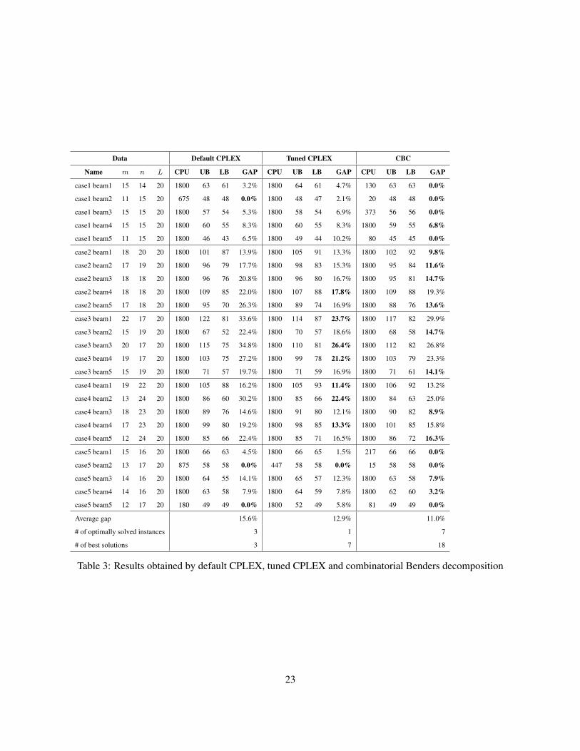
Table 2 lists the parameters that were switched from their default values. Table 3 presents the results ob-

tained on the same data set by directly solving RDP with default CPLEX parameters (“Default CPLEX”),

with tuned CPLEX parameters (“Tuned CPLEX”) and our algorithm (“CBC”). Table 3 shows that tuning

CPLEX parameters as presented in Table 2 is quite effective in closing optimality gaps for our problem. We

observe that while the average optimality gap is reduced from 15.6% to 12.9%, tuning parameters deteri-

orates solution quality for several problem instances and it decreases the number of instances that can be

21

solved to optimality from three to one. We also repeat the results obtained by our algorithm under the set

of columns titled “CBC” for ease of comparison. Similar to Table 1, numbers marked in bold correspond

to best optimality gaps found by the three approaches. We observe that our algorithm is able to provide the

best optimality gaps in 17 instances. Furthermore, our algorithm finds provably optimal solutions in seven

problem instances, which is significantly higher than the number of instances that CPLEX can solve to opti-

mality using both default and tuned parameters. These results show that our solution approach significantly

improves the solvability of the problem.

Our last experiment focuses on testing the effect of the maximum intensity level L on the performance

of our algorithm and the generated solution. In IMRT treatment planning process, fluence maps are often

generated by solving a nonlinear optimization problem and then rounding the intensity levels assigned to

bixels to integers in order to limit the delivery time. Higher values of L yield less round-off errors, and

more precise fluence maps that typically require a higher number of apertures to be delivered. Table 4

shows the results obtained by our combinatorial Benders decomposition algorithm for problem instances

that are scaled such that L ∈ {5, 10, 15} in addition to L = 20, which corresponds to our algorithm’s results

presented in Tables 1 and 3. In Table 4, bold numbers denote the problem instances that could be solved

optimally. As expected, our algorithm provides tighter optimality gaps and finds optimal solutions for more

problem instances as L decreases. In particular, our approach is able to find provably optimal solutions of 7

instances for L = 20, 8 instances for L = 15, 14 instances for L = 10 and for all 25 instances for L = 5.

This is not surprising since the problem naturally gets easier to solve as L decreases, and is polynomially

solvable for L = 1 [20].

22

Data Default CPLEX Tuned CPLEX CBC

Name m n L CPU UB LB GAP CPU UB LB GAP CPU UB LB GAP

case1 beam1 15 14 20 1800 63 61 3.2% 1800 64 61 4.7% 130 63 63 0.0%

case1 beam2 11 15 20 675 48 48 0.0% 1800 48 47 2.1% 20 48 48 0.0%

case1 beam3 15 15 20 1800 57 54 5.3% 1800 58 54 6.9% 373 56 56 0.0%

case1 beam4 15 15 20 1800 60 55 8.3% 1800 60 55 8.3% 1800 59 55 6.8%

case1 beam5 11 15 20 1800 46 43 6.5% 1800 49 44 10.2% 80 45 45 0.0%

case2 beam1 18 20 20 1800 101 87 13.9% 1800 105 91 13.3% 1800 102 92 9.8%

case2 beam2 17 19 20 1800 96 79 17.7% 1800 98 83 15.3% 1800 95 84 11.6%

case2 beam3 18 18 20 1800 96 76 20.8% 1800 96 80 16.7% 1800 95 81 14.7%

case2 beam4 18 18 20 1800 109 85 22.0% 1800 107 88 17.8% 1800 109 88 19.3%

case2 beam5 17 18 20 1800 95 70 26.3% 1800 89 74 16.9% 1800 88 76 13.6%

case3 beam1 22 17 20 1800 122 81 33.6% 1800 114 87 23.7% 1800 117 82 29.9%

case3 beam2 15 19 20 1800 67 52 22.4% 1800 70 57 18.6% 1800 68 58 14.7%

case3 beam3 20 17 20 1800 115 75 34.8% 1800 110 81 26.4% 1800 112 82 26.8%

case3 beam4 19 17 20 1800 103 75 27.2% 1800 99 78 21.2% 1800 103 79 23.3%

case3 beam5 15 19 20 1800 71 57 19.7% 1800 71 59 16.9% 1800 71 61 14.1%

case4 beam1 19 22 20 1800 105 88 16.2% 1800 105 93 11.4% 1800 106 92 13.2%

case4 beam2 13 24 20 1800 86 60 30.2% 1800 85 66 22.4% 1800 84 63 25.0%

case4 beam3 18 23 20 1800 89 76 14.6% 1800 91 80 12.1% 1800 90 82 8.9%

case4 beam4 17 23 20 1800 99 80 19.2% 1800 98 85 13.3% 1800 101 85 15.8%

case4 beam5 12 24 20 1800 85 66 22.4% 1800 85 71 16.5% 1800 86 72 16.3%

case5 beam1 15 16 20 1800 66 63 4.5% 1800 66 65 1.5% 217 66 66 0.0%

case5 beam2 13 17 20 875 58 58 0.0% 447 58 58 0.0% 15 58 58 0.0%

case5 beam3 14 16 20 1800 64 55 14.1% 1800 65 57 12.3% 1800 63 58 7.9%

case5 beam4 14 16 20 1800 63 58 7.9% 1800 64 59 7.8% 1800 62 60 3.2%

case5 beam5 12 17 20 180 49 49 0.0% 1800 52 49 5.8% 81 49 49 0.0%

Average gap 15.6% 12.9% 11.0%

# of optimally solved instances 3 1 7

# of best solutions 3 7 18

Table 3: Results obtained by default CPLEX, tuned CPLEX and combinatorial Benders decomposition

23

Data L = 5 L = 10 L = 15 L = 20

Name m n CPU UB LB GAP CPU UB LB GAP CPU UB LB GAP CPU UB LB GAP

case1 beam1 15 14 2 37 37 0.0% 5.9 50 50 0.0% 19.1 57 57 0.0% 130 63 63 0.0%

case1 beam2 11 15 1.3 29 29 0.0% 3.3 37 37 0.0% 12.3 42 42 0.0% 20 48 48 0.0%

case1 beam3 15 15 3.2 35 35 0.0% 13 43 43 0.0% 106.7 54 54 0.0% 373 56 56 0.0%

case1 beam4 15 15 7.4 33 33 0.0% 1017.9 45 45 0.0% 1800 57 53 7.0% 1800 59 55 6.8%

case1 beam5 11 15 1.9 26 26 0.0% 5.7 37 37 0.0% 24.2 45 45 0.0% 80 45 45 0.0%

case2 beam1 18 20 156.1 54 54 0.0% 1074.6 76 76 0.0% 1800 95 86 9.5% 1800 102 92 9.8%

case2 beam2 17 19 33.6 55 55 0.0% 1266.6 71 71 0.0% 1800 81 79 2.5% 1800 95 84 11.6%

case2 beam3 18 18 42.5 52 52 0.0% 1800 73 70 4.1% 1800 85 76 10.6% 1800 95 81 14.7%

case2 beam4 18 18 155.5 59 59 0.0% 1800 87 81 6.9% 1800 100 84 16.0% 1800 109 88 19.3%

case2 beam5 17 18 34.6 52 52 0.0% 1800 69 64 7.2% 1800 77 69 10.4% 1800 88 76 13.6%

case3 beam1 22 17 467.5 57 57 0.0% 1800 90 73 18.9% 1800 117 79 32.5% 1800 117 82 29.9%

case3 beam2 15 19 59.9 34 34 0.0% 837.8 46 46 0.0% 1800 58 53 8.6% 1800 68 58 14.7%

case3 beam3 20 17 516.8 55 55 0.0% 1800 81 72 11.1% 1800 97 79 18.6% 1800 112 82 26.8%

case3 beam4 19 17 499.3 55 55 0.0% 1800 81 70 13.6% 1800 96 75 21.9% 1800 103 79 23.3%

case3 beam5 15 19 30.2 40 40 0.0% 310.6 54 54 0.0% 1800 63 57 9.5% 1800 71 61 14.1%

case4 beam1 19 22 69.5 64 64 0.0% 1800 85 83 2.4% 1800 98 90 8.2% 1800 106 92 13.2%

case4 beam2 13 24 293 50 50 0.0% 1800 67 59 11.9% 1800 76 61 19.7% 1800 84 63 25.0%

case4 beam3 18 23 57.8 50 50 0.0% 1800 68 67 1.5% 1800 79 74 6.3% 1800 90 82 8.9%

case4 beam4 17 23 127.2 54 54 0.0% 1800 75 74 1.3% 1800 90 79 12.2% 1800 101 85 15.8%

case4 beam5 12 24 94.8 49 49 0.0% 1800 66 64 3.0% 1800 78 69 11.5% 1800 86 72 16.3%

case5 beam1 15 16 1.9 42 42 0.0% 3.6 51 51 0.0% 7.1 64 64 0.0% 217 66 66 0.0%

case5 beam2 13 17 1.6 35 35 0.0% 4.5 49 49 0.0% 7.5 54 54 0.0% 15 58 58 0.0%

case5 beam3 14 16 23.4 35 35 0.0% 232 50 50 0.0% 1800 60 56 6.7% 1800 63 58 7.9%

case5 beam4 14 16 3.8 29 29 0.0% 48.9 56 56 0.0% 297.8 59 59 0.0% 1800 62 60 3.2%

case5 beam5 12 17 1.8 30 30 0.0% 4.3 39 39 0.0% 12.5 46 46 0.0% 81 49 49 0.0%

Average gap 0.0% 3.3% 8.5% 11.0%

# of optimally solved instances 25 14 8 7

Table 4: Results obtained by combinatorial Benders decomposition for different maximum intensity values

24

5 Conclusion

In this paper, we described two heuristics and an exact algorithm for the problem of finding optimal de-

composition of IMRT fluence maps using rectangular apertures. Rectangular apertures can be formed by

conventional jaws already integrated in IMRT devices and these devices do not need costly multi-leaf col-

limator (MLC) systems to be used in radiation therapy. Our algorithm is based on combinatorial Benders

decomposition and it can be used to analyze the delivery efficiency of jaws-only treatment machinery. We

tested the efficacy of our approach on a set of clinical problem instances and compared our results against

the literature. Our results show that our approach is able to find higher quality solutions for most problem

instances. We also compared our algorithm’s results with direct solution of a mixed-integer programming

formulation of the problem using both default solver parameters and a parameter set that is tuned for our set

of problem instances. Our results reveal that solvability of the problem is significantly enhanced with our

combinatorial Benders decomposition scheme.

References

[1] R. K. Ahuja and H. W. Hamacher. A network flow algorithm to minimize beam-on time for uncon-

strained multileaf collimator problems in cancer radiation therapy. Networks, 45:36–41, 2005.

[2] D. Baatar, H. W. Hamacher, M. Ehrgott, and G. J. Woeginger. Decomposition of integer matrices and

multileaf collimator sequencing. Discrete Applied Mathematics, 152(2):6–34, 2005.

[3] D. Baatar, N. Boland, S. Brand, and P.J. Stuckey. Minimum cardinality matrix decomposition into

consecutive ones matrices: CP and IP approaches. Lecture Notes in Computer Science, 4510:1–15,

2007.

25

[4] L. Bai and P. A. Rubin. Combinatorial Benders cuts for minimum tollbooth problem. Operations

Research, 57:1510–1522, 2009.

[5] H. Cambazard, E. O’Mahony, and B. O’Sullivan. Hybrid methods for the multileaf collimator se-

quencing problem. Lecture Notes in Computer Science, 6140:56–70, 2010.

[6] J. W. Chinneck. Fast heuristics for the maximum feasible subsystem problem. INFORMS Journal on

Computing, 13:210–223, 2001.

[7] G. Codato and M. Fischetti. Combinatorial Benders cuts for mixed-integer linear programming. Op-

erations Research, 54:756–766, 2006.

[8] C. E. Cortes, M. Matamala, and C. Contardo. The pickup and delivery problem with transfers: For-

mulation and a branch-and-cut solution method. European Journal of Operational Research, 200:

711–724, 2005.

[9] J. Dai and Y. Hu. Intensity-modulation radiotherapy using independent collimators: an algorithm

study. Medical Physics, 26(3):2562–2570, 1999.

[10] M. A. Earl, M. K. N. Afghan, C. X. Yu, Z. Jiang, and D. M. Shepard. Jaws-only IMRT using direct

aperture optimization. Medical Physics, 34:307–314, 2007.

[11] K. Engel. A new algorithm for optimal multileaf collimator field segmentation. Discrete Applied

Mathematics, 152:35–51, 2005.

[12] K. Engel. Optimal matrix-segmentation by rectangles. Discrete Applied Mathematics, 157:2015–2030,

2009.

[13] K. Engel and A. Kiesel. Approximated matrix decomposition for IMRT planning with multileaf colli-

mators. OR Spectrum, 33:149–172, 2011.

26

[14] A. T. Ernst, V. H. Mak, and L. R. Mason. An exact method for the minimum cardinality problem in

the treatment planning of intensity-modulated radiotherapy. INFORMS Journal on Computing, 21:

562–574, 2009.

[15] M. L. Fisher. The Lagrangian relaxation method for solving integer programming problems. Manage-

ment Science, 27:1–18, 1981.

[16] J. Gleeson and J. Ryan. Identifying minimally infeasible subsytem of inequalities. ORSA Journal on

Computing, 2(4):61–64, 1990.

[17] O. Guieu and J. W. Chinneck. Analyzing infeasible mixed-integer and integer linear programs. IN-

FORMS Journal on Computing, 11:63–77, 1999.

[18] IBM ILOG CPLEX 12.2: User’s Manual. International Business Machines Corporation, 2009.

[19] T. Kalinowski. The complexity of minimizing the number of shape matrices subject to minimal beam-

on time in multileaf collimator field decomposition with bounded fluence. Discrete Applied Mathe-

matics, 157:2089–2104, 2009.

[20] T. Kalinowski. A dual of the rectangle-segmentation problem for binary matrices. The Electronic

Journal of Combinatorics, 16(1), 2009.

[21] S. Kamath, S. Sahni, J. Li, J. Palta, and S. Ranka. Leaf sequencing algorithms for segmented multileaf

collimation. Physics in Medicine and Biology, 48(5):307–324, 2003.

[22] A. Kiesel. A function approximation approach to the segmentation step in IMRT planning. Forthcom-

ing in OR Spectrum, 2009. doi: 10.1007/s00291-009-0187-2.

[23] Y. Kim, L. J. Verhey, and P. Xia. A feasibility study of using conventional jaws to deliver IMRT plans

in the treatment of prostate cancer. Physics in Medicine and Biology, 52(8):2147–2156, 2007.

27

[24] M. Langer, V. Thai, and L. Papiez. Improved leaf sequencing reduces segments or monitor units needed

to deliver IMRT using multileaf collimators. Medical Physics, 28:2450–2458, 2001.

[25] E. K. Lee, T. Fox, and I. Crocker. Optimization of radiosurgery treatment planning via mixed integer

programming. Medical Physics, 27:995–1004, 2000.

[26] E. K. Lee, T. Fox, and I. Crocker. Integer programming applied to intensity-modulated radiation

treatment planning. Annals of Operations Research, 119:165–181, 2003.

[27] E. K. Lee, T. Fox, and I. Crocker. Simultaneous beam geometry and intensity map optimization in

intensity-modulated radiation therapy. International Journal of Radiation Oncology Biology Physics,

64:301–320, 2006.

[28] Y. Li, J. Yao, and D. Yao. Automatic beam angle selection in IMRT planning using genetic algorithm.

Physics in Medicine and Biology, 49:1915–1932, 2004.

[29] G. J. Lim, J. Choi, and R. Mohan. Iterative solution methods for beam angle and fluence map opti-

mization in intensity modulated radiation therapy planning. OR Spectrum, 30:289–309, 2008.

[30] C. Men, H. E. Romeijn, Z. C. Taskın, and J. F. Dempsey. An exact approach to direct aperture opti-

mization in IMRT treatment planning. Physics in Medicine and Biology, 52(24):7333–7352, 2007.

[31] G. Mu and P. Xia. A feasibility study of using conventional jaws to deliver complex IMRT plans for

head and neck cancer. Physics in Medicine and Biology, 54(18):5613–5623, 2009.

[32] E. Niederlaender. Causes of death in the EU. Technical report, Eurostat, 2006.

[33] M. Parker and J. Ryan. Finding the minimum weight IIS cover of an infeasible system of linear

inequalities. Annals of Mathematics and Artificial Intelligence, 17:107–126, 1996.

28

[34] A. B. Pugachev, A. L. Boyer, and L. Xing. Beam orientation optimization in intensity-modulated

radiation treatment planning. Medical Physics, 27:1238–1245, 2000.

[35] H. E. Romeijn and J. F. Dempsey. Intensity modulated radiation therapy treatment plan optimization.

TOP, 16:215–243, 2008.

[36] H. E. Romeijn, R. K. Ahuja, J. F. Dempsey, and A. Kumar. A new linear programming approach to

radiation therapy treatment planning problems. Operations Research, 54:201–216, 2006.

[37] J. N. Sawaya and S. Elhedhli. A nested Benders decomposition approach for telecommunication

network planning. Naval Research Logistics, 57:519–539, 2010.

[38] R. A. C. Siochi. Minimizing static intensity modulation delivery time using an intensity solid paradigm.

International Journal of Radiation Oncology Biology Physics, 43(6):671–680, 1999.

[39] Z. C. Taskın, J. C. Smith, and H. E. Romeijn. Mixed-integer programming techniques for decomposing

IMRT fluence maps using rectangular apertures. Forthcoming in Annals of Operations Research, 2010.

doi: 10.1007/s10479-010-0767-1.

[40] Z. C. Taskın, J. C. Smith, H. E. Romeijn, and J. F. Dempsey. Optimal multileaf collimator leaf se-

quencing in IMRT treatment planning. Operations Research, 58(3):674–690, 2010.

[41] M. W. Tanner and L. Ntaimo. IIS branch-and-cut for joint chance-constrained stochastic programs and

application to optimal vaccine allocation. European Journal of Operational Research, 207:290–296,

2010.

[42] G. M.G.H. Wake, N. Boland, and L. S. Jenningsa. Mixed integer programming approaches to exact

minimization of total treatment time in cancer radiotherapy using multileaf collimators. Computers &

Operations Research, 36:795–810, 2009.

29

[43] P. Xia and L. J. Verhey. Multileaf collimator leaf sequencing algorithm for intensity modulated beams

with multiple static segments. Medical Physics, 25(8):1424–1434, 1998.

[44] Y. Zhang, Y. Hu, L. Ma, and J. Dai. Dynamic delivery of IMRT using an independent collimator: a

model study. Physics in Medicine and Biology, 54(8):2527–2539, 2009.

30