COM3600 Individual Project 3D Portraiture System Heavens - Final... · COM3600 Individual Project...

COM3600 Individual Project

3D Portraiture System

Luke Heavens

Supervised by Guy Brown

7th May 2014

This report is submitted in partial fulfilment of the requirement for the degree of Master of Computing in Computer Science by Luke Heavens.

i

All sentences or passages quoted in this report from other people's work have been

specifically acknowledged by clear cross-referencing to author, work and page(s). Any

illustrations which are not the work of the author of this report have been used with

the explicit permission of the originator and are specifically acknowledged. I understand

that failure to do this amounts to plagiarism and will be considered grounds for failure

in this project and the degree examination as a whole.

Name: Luke Heavens

Date: 07/05/2014

Signature:

ii

Abstract

The proliferation of 3D printers and their applications inevitably depend on the ease

and practicality of 3D model construction. The aim of this project is to create a 3D

portraiture system capable of capturing real-world facial data via a 360 degree head-

scanning algorithm, processing this information and then reproducing a physical

representation in the form of a figurine using custom built hardware from LEGO. The

milling machine has been constructed and proven functional by producing several

figurines, each with minor improvements over its predecessors. The implementation of

the head scanning subsystem has also been successfully completed through the

utilisation of a Microsoft’s Kinect for Windows, which generates partially overlapping

point clouds that can subsequently be aligned and merged by means of the Iterative

Closest Point algorithm. Future development and improvements to the program should

be focused in this subsystem since many advanced techniques and enhancements exist

that still remain unincorporated.

iii

Acknowledgements

I would like to start by thanking my supervisor Guy Brown for both allowing me to

complete this project and for his continued support and guidance throughout its

development.

Secondly, I would like to thank my housemates for their patience during hours of

raucous milling, particularly Claire Shroff and Ben Carr who also participated in

countless scans. In addition to this, I am incredibly grateful to the time Ben donated

whilst allowing me to utilise his skills in Adobe Photoshop that were indispensable for

the creation of many of the superb graphics and images used in the application.

Finally, I would like to thank my family for all the tolerance and support they have

shown throughout the project, especially my father who also called in many favours

that enabled the acquisition of several parts and pieces that were essential in the

construction of the milling machine.

iv

Contents

Index of Figures ............................................................................................ vii

1 Introduction .............................................................................................. 1

Background ......................................................................................................... 1 1.1

Project Aims ....................................................................................................... 1 1.2

Project Overview ................................................................................................. 1 1.3

2 Literature Review ...................................................................................... 2

Milling & 3D Printing ......................................................................................... 2 2.1

Additive Manufacturing .............................................................................. 2 2.1.1

Subtractive Manufacturing .......................................................................... 3 2.1.2

CAD & CAM ............................................................................................... 4 2.1.3

3D Modelling ....................................................................................................... 5 2.2

Representation Methods .............................................................................. 5 2.2.1

Modelling Processes ..................................................................................... 7 2.2.2

Downsampling Point Clouds ....................................................................... 8 2.2.3

3D File Formats ........................................................................................... 9 2.2.4

Microsoft’s Kinect ............................................................................................. 10 2.3

Origins & Technology ................................................................................ 10 2.3.1

Applications ............................................................................................... 11 2.3.2

Capturing Depth ........................................................................................ 11 2.3.3

Kinect fusion .............................................................................................. 13 2.3.4

Iterative Closest Point Algorithm ..................................................................... 14 2.4

Iterative Closest Point Algorithm (ICP) ................................................... 14 2.4.1

Advanced Merging Techniques .................................................................. 15 2.4.2

LEGO Mindstorms NXT .................................................................................. 18 2.5

Components ............................................................................................... 18 2.5.1

Communication .......................................................................................... 18 2.5.2

Technical Survey ............................................................................................... 19 2.6

LEGO Mindstorms NXT Firmware .......................................................... 19 2.6.1

Kinect Drivers & API’s .............................................................................. 20 2.6.2

Programming Language ............................................................................. 21 2.6.3

Processing .................................................................................................. 21 2.6.4

Summary ........................................................................................................... 21 2.7

3 Requirements & Analysis ......................................................................... 22

Analysis ............................................................................................................. 22 3.1

v

Milling Machine ......................................................................................... 22 3.1.1

Head Scanning ........................................................................................... 23 3.1.2

Languages & API’s ............................................................................................ 24 3.2

Requirements..................................................................................................... 24 3.3

Functional Requirements ........................................................................... 24 3.3.1

Non-Functional Requirements ................................................................... 26 3.3.2

Testing .............................................................................................................. 26 3.4

Evaluation ......................................................................................................... 27 3.5

4 Hardware Design & Construction ............................................................. 28

Machine Construction ....................................................................................... 28 4.1

Early Designs ............................................................................................. 28 4.1.1

Final Design ............................................................................................... 29 4.1.2

Performance Limitations ................................................................................... 30 4.2

Workpiece Material Selection ........................................................................... 30 4.3

Workpiece Size Optimisation ............................................................................ 31 4.4

Replacement Parts ............................................................................................ 31 4.5

Vertical Shaft ............................................................................................. 31 4.5.1

Milling Cutter ............................................................................................ 32 4.5.2

Carriage Runners ....................................................................................... 32 4.5.3

Preliminary Mills............................................................................................... 32 4.6

Rotational Adjustments ............................................................................. 32 4.6.1

Milling Cutter Size..................................................................................... 33 4.6.2

Eliminating Battery Reliance .................................................................... 34 4.6.3

Summary ........................................................................................................... 34 4.7

5 Implementation ........................................................................................ 35

Milling Subsystem ............................................................................................. 35 5.1

Obtaining Point Cloud Data ..................................................................... 35 5.1.1

Data Collection .......................................................................................... 35 5.1.2

Determine Optimal Axis Alignment .......................................................... 36 5.1.3

Depth Generation ...................................................................................... 36 5.1.4

Trialling Scaling Factors ........................................................................... 37 5.1.5

Unquantified Depth Removal .................................................................... 38 5.1.6

Capping Depths ......................................................................................... 39 5.1.7

Using Depth Data ...................................................................................... 39 5.1.8

Scanning Subsystem .......................................................................................... 39 5.2

Kinect Data Visualisation & Boundary Adjustment ................................ 39 5.2.1

vi

Depth capture ............................................................................................ 40 5.2.2

Combining Scan Results ............................................................................ 40 5.2.3

Merging Two Point Clouds ....................................................................... 42 5.2.4

Serialisation ................................................................................................ 46 5.2.5

3D Graphics ...................................................................................................... 46 5.3

6 Testing .................................................................................................... 48

Developing the Milling Subsystem .................................................................... 48 6.1

Developing the Scanning Subsystem................................................................. 49 6.2

7 Results & Evaluation ............................................................................... 50

Scanning Subsystem .......................................................................................... 50 7.1

Results & Correctness ................................................................................ 50 7.1.1

Tolerance ................................................................................................... 51 7.1.2

Speed .......................................................................................................... 52 7.1.3

Milling Subsystem ............................................................................................. 53 7.2

Speed & Accuracy ...................................................................................... 53 7.2.1

Results & Correctness ................................................................................ 54 7.2.2

Combined System Results ................................................................................. 55 7.3

Requirements Comparison ................................................................................ 57 7.4

User Testing ...................................................................................................... 58 7.5

8 Conclusion ............................................................................................... 60

References ...................................................................................................... 61

Appendix A: Questionnaire ............................................................................. 68

3D Portraiture System Questionnaire ......................................................................... 68

Appendix B: External Models Used ................................................................ 70

Appendix C: Milling System Schematics ......................................................... 71

C.1 Foam Optimisation ........................................................................................... 71

C.2 Milling Machine Diagram ................................................................................. 72

vii

Index of Figures

2.1 - How a cuboid can be constructed using polygons ..................................................... 5

2.2 - The relationship between the position of control points and bicubic patch shape .. 6

2.3 - Connecting points in a point cloud to construct a polygon mesh ............................ 7

2.4 - A Kinect for Windows and the technologies inside it ............................................. 10

2.5 - The infrared speckled pattern seen by the Kinect’s IR sensor ............................... 11

2.6 - Schematic representation of the depth-disparity relation. ...................................... 12

2.7 - Some perfect correspondences between example target and source point clouds ... 14

2.8 - Two point clouds before and after ICP merging. ................................................... 15

2.9 - RANSAC algorithm determining location for a best fit line .................................. 16

2.10 - Point cloud correspondences before and after pair elimination ........................... 17

2.11 - LEGO Mindstorms NXT intelligent brick and peripherals. ................................. 18

2.12 - A visual illustration of the open source SDK architecture . ................................. 20

4.1 - Early designs of the milling machine. ..................................................................... 28

4.2 - The final design of the milling shown both schematically and after construction. 29

4.3 - Demonstrating the increase in usable foam if workpiece corners are removed ...... 31

4.4 - Compairson between LEGO and metal milling cutter supports ............................ 31

4.5 - Comparison of milling cutters ................................................................................. 32

4.6 - Output from the first mill trial intended to be a cube. .......................................... 33

4.7 - Stages of milling. ..................................................................................................... 33

5.1 - The Configure System screen from the 3D Portraiture system. ............................. 35

5.2 - Three mill previews using the same model but with different axis alignments...... 36

5.3 - Converting a point cloud into an array of depths. ................................................. 36

5.4 - A comparison of edge repair techniques.................................................................. 38

5.5 - A subject rotating for their second scan. ................................................................ 40

5.6 - Two model previews where one cloud has been aligned to the Y axis ................... 41

5.7 - Two model previews before and after shoulder cropping ....................................... 42

5.8 - Difference between ICP with and without -reciprocal correspondences. .............. 43

5.9 - The construction and use of slices to generate a model preview. ........................... 47

7.1 - A point cloud produced by the system ................................................................... 50

7.2 - A comparison between 8 step and 16 step point clouds ......................................... 51

7.3 - The progression of milling machine output over the duration of the project. ....... 54

7.4 - Deficiencies in a model of Luigi, one of Nintendo’s famous game characters. ........ 54

7.5 - The production pipeline of a hooded individual. .................................................... 55

7.6 - The production pipeline of an individual wearing a Christmas hat ....................... 56

7.7 - The production pipeline of a female with her hair in a bun ................................... 56

1

1 Introduction

Background 1.1

In recent times, 3D printing has gathered considerable media attention and public

interest, as the technologies within the field continue to advance. Exciting new

applications continue to be conceived alongside these advances, with concepts ranging

from 3D printing buildings on the Moon and the fabrication of Human organs, to 3D

printed food [1] [2] [3]. It comes as no surprise then that 3D printers have started

penetrating the retail market. It is hoped, by the creators of these products, that in the

not-to-distant future, many of us will have them in our homes enabling bespoke items

such as clothes and toys to be made at our convenience [4]. The success of personalised

3D printing will rely on the ease of obtaining and constructing 3D models. Without

anything to print, a printer becomes obsolete.

Project Aims 1.2

The aim of this project will be to create a 3D portraiture system capable of capturing

real-world facial data via a 360 degree head-scanning algorithm, processing this

information and then reproducing a physical representation in the form of a figurine

using custom built hardware. Although this project will not see the construction of an

additive 3D printer (in part due to complexity, time and cost), it will attempt to

demonstrate that making customized models at home can be simple, cheap and fun

through alternative manufacturing techniques. It will ultimately determine whether the

proposed concept of 3D printing in the home could be a feasible and whether it is a

viable alternative to past manufacturing processes.

Project Overview 1.3

This project will comprise of two distinct subsystems; model generation and model

fabrication. To achieve the latter, the intention is to create a 3D milling machine (in

place of an additive 3D printer - see 2.1) out of LEGO and to use a LEGO Mindstorms

NXT intelligent brick (introduced in section 2.5), to operate its mechanical parts. If

successful, the milling system will be able to accept a 3D digital model as input and, by

coordinating the LEGO hardware, mill a figurine. In order to obtain a 3D model, an

existing digital model file could be imported or a new model constructed using the

second subsystem. The objective of this subsystem is to be able to connect to some

depth sensing technology, such as that found in Microsoft’s Kinect for Windows

(explored in 2.3), to the purpose of ‘scanning’ some object, for instance, a human head.

In the next chapter we explore concepts and techniques directly relevant to our project

through a literature review. Manufacturing processes, processes for generating 3D

models along with different model representation and storage techniques, will all be

discussed. We will also be scrutinising hardware expected to be used, in order to assess

their suitability and operational capabilities. API’s, drivers and algorithms such as the

Iterative Closest Point will all be evaluated too. Following from the literature review,

chapter 3 will analyse the choices that have been made in order to generate the final

set of project requirements which are also formally expressed. Chapters 4 and 5 explain

the design and implementation of the project including different revisions of hardware

design and comprehensive algorithm explanations. The system is then tested and

evaluated in chapters 6 and 7 before conclusions are made in chapter 8.

2

2 Literature Review

This literature review will start by examining the differences between additive and

subtractive manufacturing processes, along with the significance of computer aided

design and manufacture. Examining how manufacturing practices are changing allows

us to both evaluate the relevance of this project and also explain some of the processes

that will be implemented within it. We will then explore some of the different ways 3D

models can be represented and stored since our project will display, import and export

such models. This review will examine Microsoft’s Kinect for Windows, dissecting the

collaborative technologies incorporated into it followed by a scrutinising of the Iterative

Closest Point algorithm and associated enhancement techniques for point cloud

merging. A LEGO Mindstorms NXT kit will be responsible for the mechanical

operation of the milling machine and hence this review will also attempt to understand

the features available and its operational capabilities to assist in the utilisation of this

hardware. This chapter concludes with a technical survey of API’s and firmware.

Milling & 3D Printing 2.1

Despite the concept of 3D printing machines materializing in 1984 [5], it is only recently

that 3D printing has started to become more mainstream (see 2.1.1). When we use the

phrase ‘3D printing’, we are referring to what is otherwise known as an ‘additive

manufacturing’ process. This term allows us to make a distinction from traditional

manufacturing processes now known as ‘subtractive manufacturing’. Subtractive

manufacturing or ‘machining’ methods are well known, some examples of which are

milling and drilling [6] [7]. Since this project will not see the construction of an additive

3D printer, a traditional subtractive manufacturing approach has been chosen instead.

Both types of manufacturing could be used to produce models and figurines but this

section aims to provide the reader with a detailed understanding of the differences

between the two manufacturing classes. This section will also look at computer aided

design and manufacture to illustrate how, given a digital model, one could produce a

real-world representation. How such digital models are represented, made and stored is

the focus of discussion in chapter 2.2.

Additive Manufacturing 2.1.1

3D printing has advanced and continues to advance since the invention of

Sterolithography in 1984 by Charles Hull [5]. It is the process of constructing three-

dimensional, real-world objects through the successive deposition of layers of material.

Each layer represents a cross-sectional slice of a three-dimensional digital object [6] [8].

A Stereolithographic 3D printer utilises just one approach from a now wide variety of

processes, in order to ‘print’ a cross-sectional slice. Whilst all devices use the same

underlying principle mentioned above, the means of how a layer is formed differs from

machine to machine. Although we will not discuss in depth these approaches, the main

differences concern how the material is deposited. For example, the material used could

be squeezed, sprayed, poured, melted or otherwise applied, to form the layers [8]. In

addition to a growth in variety of deposition techniques, the diversity of printable

materials has increased also. Restricted initially to thermoplastics; metal, glass and

chocolate are just a few of the latest materials to be used [9]. Alongside advancements

in this technology, a number of exciting and innovative uses have been conceived with

applications in areas such as space exploration, fashion and medicine emerging [10].

3

3D printers have begun to appear more frequently in news articles as new technical

advances, applications and hardware are announced. Many companies such as

‘Sculpteo’1 now offer a range of online 3D printing services. Customers can buy and sell

3D designs through an online marketplace or print their own. This online 3D

community has allowed inquisitive individuals to experiment and trial the printing

process, ultimately prompting a desire in some for their own private printers. Such

personal printers have only just started to appear on the high street. The latest arrival,

known as the ‘CUBIFY Cube 3D Printer’, began selling in two major UK retail outlets

as of 2nd October 2013 with other retailers stocking shortly after [4] [11]. This project

will hopefully demonstrate the feasibility of 3D printing in the home.

In order for the 3D printing market to truly grow and gather widespread use, people

need hardware that offers flexibility whilst remaining easy to use. This process could be

assisted through the use of the aforementioned online marketplaces, smartphone ‘apps’

and applications similar to that proposed in this project. In November 2013, Microsoft

released a new 3D printing app allowing customers using its latest operating system

(Windows 8.1) to view, prepare and (assuming they have the necessary hardware) print

their models [12]. In addition, a recently funded project on crowdfunding site

‘Kickstarter’ hopes to release a smartphone accessory that will allow users to easily

generate 3D models from real-world objects through its laser based technology [13].

Both of these indicate that there is continuing progression in the area.

Subtractive Manufacturing 2.1.2

Subtractive manufacturing is, by contrast, the process of fabricating an object by

obtaining a solid block of raw material and then machining away excess material from

it [7] [8] [14].

Machining is a far-reaching term that covers many different processes and tools. Some

of the major machining processes are: Boring, Cutting, Drilling, Milling, Turning and

Grinding [15]. Each process specialises in completing different tasks but may be used

together to complete complex projects. Drilling is the most widespread machining

process which allows the creation of holes [16]. For the purposes of this project however,

we are interested in Milling.

“Milling is the machining process of using rotary cutters to remove

material from a workpiece advancing (or feeding) in a direction at an

angle with the axis of the tool.” [17]

Milling may be performed in two manners. The first, known as horizontal milling,

describes a movement where the axis of the tool is parallel to the surface of the

workpiece. The second, known as vertical milling (or face milling), describes a

movement where the axis of the tool is perpendicular to the surface of the workpiece.

The proposed milling method for this project would be face milling [18] [19].

1 Accessible at: http://www.sculpteo.com/en/

http://www.sculpteo.com/en/

4

CAD & CAM 2.1.3

Both types of manufacturing can be used with Computer Aided Design (CAD) and

Computer Aided Manufacture (CAM); fundamental components to the concept of

Computer Integrated Manufacture (CIM). The objective of CIM is to automate a whole

manufacturing process, from factory automation (e.g. with the use of robots),

manufacturing and planning control, business management and finally, CAD/CAM. By

automating the manufacturing process, time and money are saved whilst

simultaneously increasing accuracy, precision, consistency and efficiency [20]. This

concept accurately describes many desirable traits in our system. The reader should be

able recognise many principles outlined below within our system requirements in 3.4.

“Computer aided design involves any type of design activity which

makes use of a computer to develop, analyse or modify an engineering

design.” [21]

Using computers to aid the design process provides many advantages. The productivity

and freedom of design can be substantially increased, since the creation can be

visualised before fabrication. Modifications can then be made without as many

prototypes thus reducing production time and waste material. Compared to

conventional methods, the speed and accuracy of a design can be significantly

improved, particularly since dimensions and attributes can be altered without repeating

or redrawing any components. Previewing the model on-screen can help reduce errors

by allowing the design to be viewed at a much higher accuracy than could be drawn.

Finally, the process of designing through a CAD system allows costs, dimensions and

geometry to all be collated for later use across a range of a CAM processes [21] [22].

Computer aided manufacturing is a very broad term that describes any manufacturing

process that is computer aided, whilst not relating to the design phase. There are a vast

range of CAM machines, each excelling in different scenarios. If manufacture is required

on a mass scale (e.g. in the production of cars), then specialised machines can be

created to significantly decrease cost and time. However, these machines are often

unadaptable and will be little or no use for another product. By contrast, personal or

stand-alone CAM machines are generally designed to be as flexible as possible but at

the expense of efficiency [20] [22].

Since the mid twentieth century, CNC (computer numerical control) machines have

been used to automate machine tools that were previously operated manually.

Nowadays, almost all machining processes can be carried out by some variant of a CNC

machine. A CNC machine requires a computer to first convert a digital design into

numbers which can then be used to control machining tools. Whilst a computer is able

to use and create designs in a range of formats, machining devices require models to be

represented in a form that can be understood in terms of movement. The model must

therefore be converted into coordinates (numbers) representing depths and positions in

space. The computer will communicate with an interface which is responsible for using

this data to provide the machine with step by step movements. These instructions will

be sent to the machine as electronic signals. The machine will use these signals to

control the , and position of the machining tool. Some machines allow variable

speed and control through additional axes [20] [23].

“A CNC milling machine or router is the subtractive equivalent to the

3D printer” [14]

5

3D Modelling 2.2

3D computer graphics are founded on the realisation that shapes and geometry can be

represented mathematically as structured data [24]. 3D models are designed and created

for many reasons in a multitude of fields, such as entertainment, in the form of games,

films and art; and for simulations, to virtually realise situations that may be difficult or

unsuitable for real-world investigation [24] [25]. In this project 3D models will be

displayed, imported and exported, hence an understanding is important.

Representation Methods 2.2.1

3D models are geometric descriptions of objects. There are however many different

ways to represent these descriptions, the most appropriate of which, depending on the

object’s intended use. If a model were to be used in a digital scene (e.g. a computer

game) then properties such as colours, textures and transparency would need to be

considered. The way objects interact and move can also be programmed by modifying

the descriptions of the objects over a period of time [26].

Due to the immense diversity of objects that can be displayed, there is no single

representation method that best describes all of them. The most predominantly used

depiction of an object is through a mesh of polygons due to its simplicity. Each polygon

is constructed from a list of coordinates which define the vertices. The surfaces or

‘facets’ of these polygons are connected to represent the exterior or ‘boundary’ of the

object. Implementations differ, with some variations explicitly defining the edges of the

polygons, whilst others doing so implicitly. An edge based approached can reduce the

processing requirements for complex objects, as edges are only processed once. The

stages in the representation of a simple cuboid can be seen in Figure 2.1.

Figure 2.1 - How a cuboid can be constructed using polygons [27].

One of the main inadequacies with the polygon mesh representation is its inability to

accurately define curved surfaces. The quality of curve approximations can be improved

by using more polygons to represent it. This, however, is done at the expense of render

time and memory. Another potential issue is that we do not always know which

polygons share a vertex unless the data is stored in a specific way. This information is

needed in shading algorithms for example. Despite this, due to the flexibility and fast

rendering times, polygonal modelling is the preferred method for object representation

[25] [26].

6

Bicubic parametric patches are an alternative way of representing the boundaries of a

model [28]. One key advantage over polygonal representations is the ability to represent

a curve without approximation. This representation uses a mesh of patches. Each patch

(unlike the polygonal shape) is a curved surface, where every point is defined in terms

of two parameters in a cubic polynomial. The most common way of calculating this

polynomial is by using 16 control points and generating a unique description. If a single

control point is changed, the curve could appear completely different [29]. This

relationship is demonstrated in Figure 2.2. Four of the control points represent the

corner points of the patch whilst the others describe the curve.

The biggest hurdle in implementing this method of representation is that each patch

must take its neighbouring patches into consideration [28]. Assuming the complexity in

generating and constructing the model description can be overcome, objects can be

represented very concisely. Strictly speaking, a near-infinite number of polygons could

only approximate some curves that can be represented exactly with a single curved

patch [29]. The ramifications of this are clear to see, particularly with respect to

memory usage and processing time.

Figure 2.2 - The relationship between the position of control points and the shape of a patch [29].

So far we have only seen boundary representations of objects. Although we will not use

other types of modelling in our project, a brief overview of some alternative techniques

have been included for completeness. For simulations and specialised applications where

boundary representations are insufficient, solid models can be made. This type of

modelling is known as a volume representation. Constructive solid geometry (CSG) is

one such method. Complex objects are constructed by applying a series of union,

intersection or difference operations on several primitive objects such as spheres,

cylinders and cuboids. These complex objects can in turn be used to create increasingly

complex shapes [29] . [30]

Implicit functions allow exact representations of objects using formulae and math. To

construct a sphere you could use the formula x2 + y2 + z2 = r2 for example. This

method is however only useful for a limited number of shapes. Other representation

methods exist such as space subdivision techniques. These involve dividing up object

space and storing what parts are present in each. This is usually done using a

secondary data structure for uses in graphics work such as ray tracing2 [28].

2 A technique for generating an computer graphics frame by tracing the path of a light ray.

7

Modelling Processes 2.2.2

Models can be created in a number of ways depending on the modelling representation

chosen. They can be manually created through modelling software; generated

automatically, through procedural generation (algorithmically) or by mathematical

definition; made by sweeping3 2D shapes; or finally, through the scanning of an object

from the physical world [25] [26]. The construction of models in this project will be done

using the final approach. With the assistance of a depth scanner (see 2.3.5), several

point clouds can be obtained and merged together (see 2.4) permitting the generation

of a 3D model.

“[A point cloud] is a bunch of disconnected points floating near each

other in three-dimensional space in a way that corresponds to the

arrangement of the objects and people in front of the Kinect.” [31]

A point cloud is not a 3D model. It has no defined boundary, it cannot be textured and

it can’t be rendered without gaps and holes [32]. Points in a point cloud can however be

connected to form polygons or used as control points to make parametric patches [28].

To provide the reader with an insight as to how model generation from point cloud

data could be achieved, we now consider one approach to creating a polygon mesh.

Depending on the file format desired (see 2.2.4) and the exact object representation

method selected, the algorithm for completing this process will vary. We assume here

that sufficient pre-processing has been performed (e.g. downsampling - see 2.2.3).

The goal, in this example of model generation, is for each point in the cloud to be used

as vertices of polygons which in turn will become facets of the mesh structure. Once all

the polygons are connected, we consider the 3D model fully formed. To generate the

mesh using triangular polygons, each depth point must be examined in sequence and its

three nearest neighbouring points located4. Using these four points, we can form two

triangles which can both then be added to the model description [31]. This process can

be seen in Figure 2.3. The sequence of which points are selected and the order in which

the vertices are defined must be carefully chosen to ensure that each facet normal can

be correctly calculated [32]. This also necessitates a sufficiently high cloud resolution.

Figure 2.3 - Connecting points in a point cloud to construct a polygon mesh [31]

3 Sweeping is the process of making a model by moving a cross-section (generator object) along an arbitrary trajectory through space [29]. 4 This is an example of a nearest neighbour search algorithm, which “when given a set S of

points in a metric space M and a query point q ∈ M, finds the closest point in S to q” [79]

8

Downsampling Point Clouds 2.2.3

At several points throughout the project downsampling will be required. The purpose of

downsampling or ‘subsampling’ is to reduce the amount of data representing an object

(e.g. pixels in an image, or points in a point cloud) whilst trying to maintain, as

accurately as possible, the initial data. In certain situations, the effects of outliers and

errors become less prominent (i.e. the data is smoothed) by downsampling. This occurs

because the erroneous data is dissipated amongst the valid, since the correct data is

usually more numerous. In this section we discuss several downsampling techniques.

2.2.3.1 Random Downsampling

Random downsampling is arguably the easiest downsampling approach. The desired

size of the final subset of points is first chosen. Random points are selected from the

point cloud and retained to represent the final cloud. Once a point is selected it cannot

be selected again and as soon as the predetermined number of points has been selected

the subset is complete. The major flaw with this method is that some areas of the cloud

may be oversampled i.e. too many points still remain, whilst other areas of the cloud

may be undersampled i.e. too few points still remain.

2.2.3.2 Systematic Downsampling

Systematic downsampling is another simple approach to downsampling. Some interval

is first chosen indicating how frequently a point should be retained whilst iterating

through each point in the cloud. The results of this approach vary depending on the

dataset. If the points are initially uniformly distributed and contain no underlying

patterns (for example an outlier occurring every points) then the downsampled data

will be evenly distributed account of the initial data. If however, the original data

contains areas with large point density differences or contains underlying patterns; this

approach could inadequately represent the data [33].

2.2.3.3 Voxel Grid Downsampling

Voxel grid downsampling first splits the object space into a three-dimensional grid (one

could imagine collection of stacked cube boxes). Considering point clouds, this dictates

that all points will lie exclusively within a single voxel. Each voxel could contain more

than one point. After dividing the point space, each voxel will be assigned a value that

represents an approximation of its containing points, usually obtained through

averaging techniques. These values define the downsampled dataset. An alternative

version assumes the voxel centre as the approximated value rather than averaging the

points within it. Despite being fast to compute, this approach is less accurate [34].

2.2.3.4 Poisson Disk Downsampling

Poisson Disk downsampling is a technique whereby points are only permitted in the

final subset of points if they are at least a minimum distance apart from any other

point. This can be visualised in 2D by drawing some radius around a point to form a

disk arising to the algorithm’s name. Despite this, the algorithm can be used in 3 or

higher dimensions [35]. Many different implementations of this algorithm exist and it is

used in a wide range of applications too. Random object placement and texture

generation are popular examples [36]. Here, we consider its basic principles for

downsampling a point cloud. Points are first selected at random from the point cloud.

If any points are located within the minimum radius, the point will be excluded from

the final point cloud, if not, it will be retained. Once all points have been checked all

points remaining form the downsampled subset [37] [38].

9

2.2.4 3D File Formats

There are many different 3D file formats, each providing its own advantages and

disadvantages depending on the intended end use for the contained model(s). Three

popular formats considered for use during this project to import and export files were

STL, PLY and OBJ. All three are outlined below:

The STL (Sterolithography) file format (commonly used in CAD) implements the

polygon mesh representation described earlier [39]. An STL file can define multiple

objects and for each, a list of all its facets. Each facet is in turn described by its

normal5 and a list of all the vertices that define it. STL assumes all polygons are

triangles and therefore each facet should contain three vertices expressed in terms of ,

and [40]. There are two alternative encodings, ASCII and binary. The ASCII format

is useful for testing and situations where the user would like to view the file contents. It

can however produce large files which become difficult to manage. The binary format

represents the same information in a less verbose manner. It simply lists groups of

twelve floating point numbers for each triangle ( , and for both the polygon normal

and its three vertices) [41].

Polygon File Format (PLY) is an alternative file format used more in computer

graphics than in CAD. Like the STL format, it stores objects using the polygonal

representation method and it can be represented in both ASCII and binary formats.

However, PLY is more flexible. It can store polygons of different degrees and describe

additional properties such as colour, transparency and texture coordinates. Another key

difference is in regards to the way polygons are represented. Collections of both vertices

and faces are made, where each face is described by a list of the vertex indices that

construct it. This allows different polygons to share the same vertex and prevents

duplicate data thus reducing the file size [42].

The Wavefront OBJ file format (so named due to its development by Wavefront

Technologies) is another widely used file format, predominantly in computer graphics.

Unlike the previous two methods, it allows lines and curves to be accurately

represented in addition to polygons. The composition is similar to PLY but data types

are pre-defined. There are several vertex data types for example, one of which being

geometric vertices. Other elements (such as a face) could then be defined in terms of

more primitive types. This file format can be harder to understand due to the number

of different data structures and the advanced descriptions stored (e.g. curves and

texture mapping) [43].

After comparing the file formats it was decided that STL files should be used as the

primary supported file format, in part since the other file formats added extra

unnecessary complexity. Properties such as colour and texture coordinates are not

needed for example. The full reasons for this decision are discussed in section 3.2.4. If

the project were developed further however, an opportunity to add additional file

format support is available.

5 The facet normal is often redundant since it can be deduced using the order in which the vertices are declared. Some software packages therefore set all normal vectors to (0,0,0), although this is discouraged. Others instead use it to record shader information [40].

10

2.3 Microsoft’s Kinect

In this section we will examine Microsoft’s Kinect for Windows. We will dissect the

technology it contains, research its origins, learn its significance across a range of fields

and discuss the range of applications into which its technology can be used.

Due to its relevance in this project, particular focus will be given to the Kinects depth

sensing technology and how the data obtained through it can be used to construct 3D

models.

2.3.3 Origins & Technology

Microsoft’s Kinect for Windows was originally designed as a peripheral for the Xbox

360 gaming console as new way for gamers to interact with virtual environments [44].

Although not initially usable with computers, after becoming the fastest selling

computer peripheral in history, it wasn’t long before open source communities and

hackers managed to gain access to the device [31]. Many researchers in the fields of 3D

modelling and mapping realised the potential of low-cost and widely available depth

technology and quickly conceived applications and projects to harness the device’s

abilities [45]. Microsoft eventually released an official software development kit (SDK)

which resulted in many developers incorporating the Kinect into their systems.

Inside the Kinect there are three main technologies, namely a colour video camera, an

IR (infrared) projector and an IR camera [46]. The infrared emitter and sensor are

configured to be used in unison to create a depth camera, the workings of which will be

explained in 2.3.5. In addition, the Kinect contains a multi-array microphone, a three-

axis accelerometer and a vertical tilt motor. The multi-array microphone consists of

four microphones that together allow an audio source (such as human speech) to be

both detected and located relative to the device [46]. The accelerometer is intended to

be used primarily to determine the device’s orientation with respect to gravity [47].

In Figure 2.4 it is possible to see both an external and internal view of the device. The

microphone array is shown in purple, the accelerometer and tilt motor in blue and

finally the three light technologies are shown in green. It should be also noted, that a

key difference between the Kinect for Xbox and the Kinect for Windows, is the

introduction of a feature known as ‘Near Mode’. This allows objects to be ‘seen’ as close

as 40 centimetres to the device [46].

Figure 2.4 - Left: A Kinect for Windows [48], Right: The technologies inside the Kinect [49].

The Kinect does however have certain limitations and restrictions. Its field of view is

restricted to 57 horizontally and 43 vertically (±27 vertical tilt), whilst its depth range

is restricted from 80cm to 400cm (40cm - 300cm with near mode). In addition, the

Kinect cannot be used in bright sunlight due to the infrared interference and the

maximum depth resolution is 640 by 480 [50]. Despite these limitations, the Kinect

remains a powerful tool, made more favourable by its availability and low cost.

11

2.3.4 Applications

Face recognition, 3D object scanning, motion tracking, skeleton tracking and gestural

interfaces are just some of the applications of this device [44]. Using depth information

produced by the device forms the basis for the majority of projects into which the

Kinect has been incorporated. Cameras and other implemented technology have been

available to developers in the past, but the depth hardware included in the Kinect

provides a low-cost alternative to previously expensive and specialised hardware [31].

Like the 3D printers, as the technology continues to advance (in next generation

models for example), an increasing number of uses for it will be imagined.

2.3.5 Capturing Depth

As previously mentioned, the depth sensing process relies on the collaboration of two

pieces of hardware, an infrared emitter and an infrared sensor. The sensor must first

detect a ‘speckled’ pattern formed from the projected infrared light reflecting back off

objects in a room. This pattern will then be compared to a reference image which is

stored in the Kinects memory. The reference image shows the position of the dots that

create the speckled pattern at a known distance from the sensor [31] [45].

By identifying unique arrangements amongst the dots and then calculating their

distortion (i.e. the difference between their location in the reference image and in the

detected pattern), the Kinect can determine its distance to the particular arrangement

of dots. This principle works regardless of whether the object reflecting the pattern is

closer or farther than the distance used to calibrate the reference image [31] [45]. An

example of an emitted speckled pattern can be seen in Figure 2.5 and a close up

showing how the speckled pattern is made from a large number of scattered infrared

points or ‘dots’ can be seen from an enlarged section.

Figure 2.5 - The infrared speckled pattern seen by the IR sensor. The image on the left shows a close-up of the boxed area. [44].

The technique used to obtain depth readings is known as a triangulation process. It is

so named due to the three elements used in the measurement, namely the emitter,

sensor and object, which, when drawn schematically, form a triangle. Since the relative

geometry between the emitter and sensor are known, if we can determine the object’s

location relative to them, we can mathematically compute the distance from the device

to it [44].

12

A simplified schematic can be seen in Figure 2.6 where we assume only one dot is being

projected. The diagram is situated in the , plane, where some distance in

represents a distance from the Kinect. It is possible to see the infrared sensor at point

and the infrared emitter at point which have both been located on the axis, i.e.

where distance from the Kinect is zero. We will now consider two scenarios. The first

occurs during the production of the reference image, where a beam of light is fired from

the emitter to a reference plane at a known distance from the device ( ). This is

represented by the line from to . The light is reflected at towards the sensor at .

During Kinect calibration, the location of the dot relative to is stored, along with .

Figure 2.6 - Schematic representation of the depth-disparity relation [45].

In the next scenario (and any subsequent scenarios), we can use this information to

determine how much closer or farther an object is to the Kinect in relation to the

reference plane. Consider this time an object that is placed closer than the reference

plane that interrupts the same light beam fired in the first scenario. As the light is

being reflected from point rather than point , from the sensors perspective at , the

reflected dot will have been displaced along the axis.

Based on the focal distance of the IR sensor ( ), the disparity distance ( ) between the

reflections from and , the distance from the device to the reference plane ( ) and

the distance between and ( ), we can calculate (the distance from the device to

the object). Note that , and are determined during the device calibration [45].

Using the principles of triangle similarities we have the equation:

Equation 2.1

We also have a second formula from the lens equation:

Equation 2.2

Substituting from equation 2 into equation 1 and rearranging gives us the expression:

Equation 2.3

13

Using our calculated depth value and a couple of additional parameters measured

during the calibration phase, we can calculate the full Cartesian coordinates of each

point. The process described on this page is repeated for a multitude of dot patterns

emitted from the projector in order to build a complete depth image for a scene [45]. A

dot can be matched to a reference dot pattern using methods such as normalized cross

correlation because the patterns are sufficiently dissimilar [44].

Once we have gathered several depth readings and converted these into three

dimensional points, we are left with a point cloud.

2.3.6 Kinect fusion

Kinect Fusion is a tool included in Microsoft’s official SDK for the Kinect. It allows 3D

object scanning and model creation by combining depth data results over a period of

time to create a static 3D construction [51].

First, raw depth data is obtained from the Kinect as described earlier. After obtaining

this data a ‘bilateral filter’ is applied. This filter helps reduce noise within the depth

data, formed through erroneous readings and discrepancies. It works by replacing each

depth value with a weighted average of surrounding values. Despite reducing the level

of detail, a bilateral filter will smooth out errors whilst preserving boundaries [52].

The depth data is then converted into two separate maps, a vertex map and a normal

map. The vertex map contains a scaled set of Cartesian points where the point

coordinates are expressed in metres. This is done using the infrared camera’s calibration

information. The normal map is created by iterating through each vertex and looking

at its closest two neighbours. These three points create a triangle for which a normal

can be calculated. The normal is then assigned to the current point [51] [52] [53].

If existing model data exists from previous iterations of the algorithm, the new point

cloud is rotated and aligned with the existing model so that the data can be merged.

This is done by applying a variation of the Iterative Closet Point (ICP) algorithm

discussed in section 2.4 using both the vertex and normal maps from the current scan

and the vertex and normal maps from the model constructed so far. Rather than

finding the closest points however, the Kinect Fusion algorithm uses the assumption

that (since running in real-time) depth readings will be close together. It finds links

between the orientations of points in the current cloud with previous ones. A ‘projective

data association’ is used to find these associations. This information describes the

change of camera position relative to the object known as the camera ‘pose’ [52] [53].

The unfiltered depth data is then merged with the current model using the known

camera pose. The unfiltered version of the depth data is used as details may be

otherwise lost. Since multiple iterations of the algorithm are made with differing data,

any errors or discrepancies should be lessened. This algorithm is performed in real-time

at a rate of approximately 30 times a second. The model is usually rendered during this

capture process as well using 3D rendering techniques to smooth the model [51] [52].

The final output of a Kinect Fusion scan can either be a point cloud, a volume

representation or the data can be converted to a mesh i.e. a boundary representation of

the object in a format such as STL (refer to 2.2 for more information on these) [51].

14

2.4 Iterative Closest Point Algorithm

The Kinect (and similar depth scanning devices) are unable to capture 360 degrees of

an object from one position, just like our eyes. Therefore, in order to build a 360 degree

model, a series of discrete point clouds - each produced by a different scan and each

representing a different perspective, relative to the model - need to be created and

merged to form a single large point cloud. In this section we will discuss the Iterative

Closest Point algorithm (ICP) which provides one approach for merging point clouds

and some advanced techniques that can enhance this algorithm.

2.4.3 Iterative Closest Point Algorithm (ICP)

The purpose of this algorithm is to transform one of two point clouds in such a way,

that it correlates with the second. We shall refer to the former as the ‘source’ cloud and

the latter as the ‘target’ cloud. During the following initial explanation, let us assume

that both clouds are representing the same part of the same object but where the

source cloud has been translated and rotated with respect to the target.

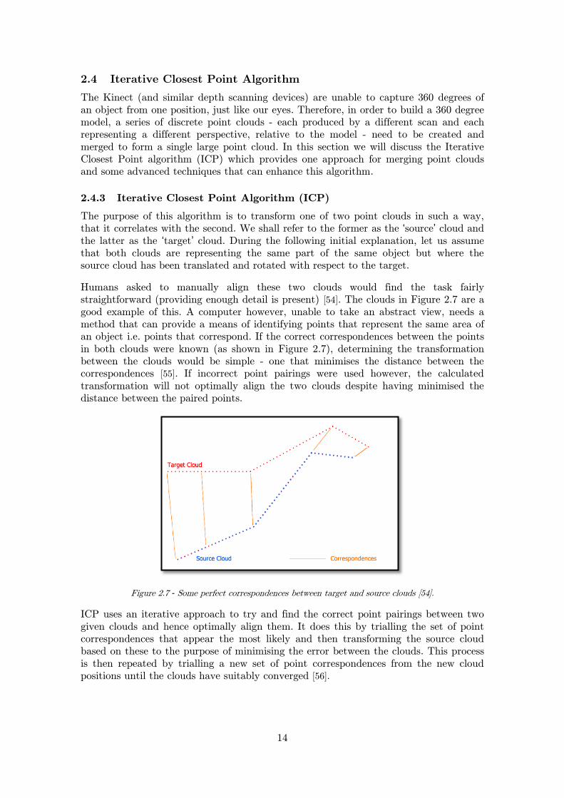
Humans asked to manually align these two clouds would find the task fairly

straightforward (providing enough detail is present) [54]. The clouds in Figure 2.7 are a

good example of this. A computer however, unable to take an abstract view, needs a

method that can provide a means of identifying points that represent the same area of

an object i.e. points that correspond. If the correct correspondences between the points

in both clouds were known (as shown in Figure 2.7), determining the transformation

between the clouds would be simple - one that minimises the distance between the

correspondences [55]. If incorrect point pairings were used however, the calculated

transformation will not optimally align the two clouds despite having minimised the

distance between the paired points.

Figure 2.7 - Some perfect correspondences between target and source clouds [54].

ICP uses an iterative approach to try and find the correct point pairings between two

given clouds and hence optimally align them. It does this by trialling the set of point

correspondences that appear the most likely and then transforming the source cloud

based on these to the purpose of minimising the error between the clouds. This process

is then repeated by trialling a new set of point correspondences from the new cloud

positions until the clouds have suitably converged [56].

15

Prior to this algorithm, the data is first pre-processed or ‘cleaned’. During this step,

erroneous or unwanted data is removed in order to improve the success of the

algorithm and results [57]. Downsampling methods such as those discussed in 2.2.3

would be included at this point. The iterative process is now able to commence. In its

most naïve form, pairings are made between points in the target and source clouds by

matching each point in the source cloud to the closest point in the target. In section

2.4.4 we see numerous techniques for improving this stage by, for example, using a

specially chosen subsets of points to increase accuracy and nearest neighbour search

time improvements [55].

The error between the two clouds can be calculated based on the distances between the

pairings. By combining transformations across 6 degrees of freedom (translations and

rotations about each of the , and axes), a single complex transformation consisting

of a rotation and translation can be made to try and best reduce the error between

each pair of matching points. Applying this transformation to the source cloud should

align the point clouds closer together. This process is then repeated over several

iterations, each time reducing the error further still, until they become similar enough

to satisfy a defined stopping condition or have converged [54] [58].

Section 5.3.6 provides a detailed account of this project’s implementation of the ICP

algorithm. Two clouds merged using this algorithm can be seen in Figure 2.8 below:

Figure 2.8 - Two point clouds before (left) and after (right) ICP merging. Both images show the two point

clouds from different angles. The clouds were captured 45 degrees apart.

2.4.4 Advanced Merging Techniques

Estimating the optimal transformation for a given iteration can be calculated very

quickly due to complexity [55]. By contrast however, the pairing phase takes

quadratic time complexity (assuming both clouds have points) since every

point in the source must be compared with every point in the target [59].

In this section we discuss how reducing the computational complexity of finding the

nearest neighbouring points can be achieved, how the number of points used in the

paring process can be reduced and also how we can reduce the number of iterations

needed before the point clouds converge. The more advanced and often more complex

techniques both meet these goals and increase (or at least do not reduce) the quality of

the final results. The final performance of an ICP algorithm can be analysed from its

speed, tolerance to outliers and the correctness of the solution [56].

16

Prior to performing the ICP, the point data could be assembled into a secondary data

structure, for example a k-dimensional tree. This is a specialised example of a space

partitioning method that recursively divides the point space using hyperplanes6 and is

commonly used with ICP [59]. Although a secondary data structure initially takes extra

time to construct and consumes extra memory, nearest neighbour searches during the

pairing phase of each iteration can now be performed at an improved average

complexity of [55] [56]. Although we will not discuss these secondary data

structures in depth, the reader should be aware that several alternative options exist

such as vp-trees and the spherical triangle constraint nearest neighbour [59].

In addition to improving the speed at which pairings are made, reducing the number of

points that need to be matched will also increase the efficiency of the algorithm.

“A reduction of the number of points [in the point cloud] by a factor N

leads to a cost reduction by the same factor for each iteration step.” [60]

Point elimination can be achieved using techniques such as RANSAC (Random Sample

Consensus). RANSAC randomly selects N points at random to estimate model

parameters (where N provided by the user). A count of the points conforming to this

model is made and recorded. After several iterations, the model parameters producing

the highest point count are deemed the best. Any points that do not conform to the

model are considered outliers and hence are not used in the matching phase [54] [61].

This algorithm is an example of outlier filtering method [62].

In Figure 2.9 it is possible to see a simple 2D example of this algorithm. A set of points

containing both inliers (blue) and outliers (red) is visible. In the centre image, two

points (green) have been randomly selected and a line of best fit produced. In the right

image, indicating a second iteration, another two points have been randomly selected

and again, a line of best fit produced. After comparing the number of points enclosed

within both shaded areas (indicating some tolerance threshold) the RANSAC algorithm

would select the second line to best describe the data due to the higher point count.

The number of iterations required is determined by probability calculations [61].

Figure 2.9 - RANSAC algorithm determining location for best fit line. Left shows initial point set, middle shows line produced from iteration one and right shows results from iteration two.

6 This is a plane one dimension smaller than the containing space e.g. a 2D plane in 3D space.

17

Some techniques aim to improve the overall convergence time i.e. reduce the number of

iterations needed, although many require more computational power on each iteration.

Weighting systems (of which there are a wide variety), are used to help the program

decide which points are more likely to be related than others. Some point similarities

will be ignored or ‘rejected’ if they are deemed significantly less important. Weights can

be based on point normals or the magnitude of pair distances for example [56] [63].

Given a situation where the two point clouds only have partially overlapping

correspondences (as will be the case in our project) many of the pairings will be invalid

and unhelpful in correctly aligning the clouds. One simple solution to remove these

unwanted pairings is to introduce the concept of back projection or -reciprocal

correspondence. This is another example of pair rejection. As explained by Chetverikov

and Stepanov in [63]:

“If point ∈ has closet point ∈ then we can back-project onto

by finding closest point ∈ . We can reject pair if ‖ ‖ .”

In Figure 2.10 we can see how pairings would be removed with a threshold . In

this instance only one-to-one correspondences are allowed. A threshold that is greater

than zero is often desirable as it provides the system with greater tolerance for error

[63].

Figure 2.10 - Point cloud correspondences. Left showing all initial correspondences, right showing those remaining after pair elimination [57]

We have already seen that the computation time can be reduced by analysing fewer

points. Downsampling the data too much however, can cause loss of precision during

alignment. The multi-resolution approach suggested by Timothée Jost and Heinz Hügli

[59], describes a method that avoids a compromise between efficiency and accuracy.

They show that by starting with greatly downsampled data during initial iterations and

continuously increasing the number of points over time the efficiency can be greatly

increased without detriment to the quality of the alignment.

The reader should be aware that in order to maintain the focus of the report, here we

have only discussed a handful of techniques and that many other different variations of

the ICP exist. Some point clouds are treated as rigid bodies or can be scaled [60],

alternatively point-to-plane or normal projecting algorithms can be used in place of

point-to-point distance measurements [56] [64].

18

2.5 LEGO Mindstorms NXT

In 1998, LEGO launched the first of their ‘Mindstorms’ kits. These kits contain LEGO

pieces, electronic components and software that can be used together to create fully

customisable and programmable robotic models. In 2006, LEGO released a second-

generation product known as the LEGO Mindstorms NXT kit. In addition to the

intelligent brick (see below), a variety of sensors such as touch and ultrasonic are

included with the set. This kit was upgraded in 2009 with the release of LEGO

Mindstorms NXT 2.0. This upgrade provides greater precision and additional sensors

such as colour [65]. It is this version that is expected to be responsible for the

mechanical operation of the milling machine in our project. On the 1st of September

Lego Mindstorms EV3 was announced as the third-generation Lego Mindstorms kit.

2.5.3 Components

The primary component in the Mindstorms NXT set is the intelligent brick, or simply,

the NXT. The brick is responsible for coordinating all the other electronic components

via its four input and three output ports. It is first programmed (or sent a program

from another device), which when executed, allows it to independently make decisions,

take measurements and perform movements. The kit contains three servo motors and

four sensors; touch, sound, colour and ultrasonic [66]. These components can be seen in

Figure 2.11. The advantage of a servo motor is that it can use built-in rotation sensors

to determine how many degrees the output shafts have turned. This allows for

reasonably precise movements. Like the sensors however, there are noticeable

limitations regarding the accuracy of the device [67].

Figure 2.11 - LEGO Mindstorms NXT intelligent brick and peripherals [68].

2.5.4 Communication

There are multiple ways of programming the NXT. Simple programs can be created on

the brick itself, programs can be written elsewhere and sent to the device for execution,

or the program could be executed on another device (such as a computer) which

remotely controls the NXT [65]. There are a numerous firmware choices available for

installation on the device, each providing support for different programming languages

and a variety of advantages and features depending on the intended use (see 2.6). Most

allow the device to be linked to a computer either by a USB cable or via a Bluetooth

connection. Whilst a USB connection is faster and can be more reliable, Bluetooth

allows extra flexibility in terms of mobility and is supported on a wide range of devices

(such as mobile phones) [69].

19

2.6 Technical Survey

Due to operational experience and the technologies required, it has been decided that

this project will be written in either C++ or Java. In this section we therefore examine

some of the API’s and Firmware available for each language along with their

advantages. This section allows comparisons between the available technologies to be

made whilst also providing an insight into the limitations of each.

2.6.3 LEGO Mindstorms NXT Firmware

In the last section we examined the LEGO Mindstorms NXT kit and mentioned the

variety of firmware choices available. Since the project will be written in either C++ or

Java, a firmware choice for each has been scrutinised below. These two were deemed

most suitable for this project after investigations into a number of alternative firmware

options were performed. Using feature lists, descriptions, benchmarking information and

user reviews available on the Internet, enabled the two options to be singled out.

2.6.3.1 leJOS NXJ

leJOS NXJ is a Java based firmware replacement. It is installed onto the NXT brick

and establishes up a Java virtual machine. In addition, a collection of Java classes,

optimised for the NXT, are provided allowing Java programs written on a computer to

communicate effectively and efficiently with the device. There are a number of

advantages to using leJOS as opposed to other firmware. It has highly accurate motor

control (see later), supports multithreading, allows connections over both Bluetooth

and USB, supports listeners and events, provides floating point Math functions and,

being Java based, has inherent advantages such as being both object-orientated and

portable [70].

2.6.3.2 NXT++

NXT++ is an interface written in C++ that also allows connections via Bluetooth and

USB to a LEGO Mindstorms brick. It too has a collection of files that can be imported

into an application to allow connections to be established with the NXT with relative

ease. Despite the range of features and functions provided with NXT++ being

substantially limited by comparison, all tools needed for this project are provided [71].

2.6.3.3 Comparison

Like leJOS, NXT++ is the result of an open source project but of a considerably

smaller size. For this reason, the amount of documentation and information is in

considerably less abundance. Each has additional features that the other does not, such

as allowing support for multiple devices and providing GPS device support [70] [71].

Since this project will not require all these features, their presence has not influenced

decisions taken. One of the claims by leJOS is that it provides a high accuracy of motor

control. Since accurate motor control is paramount to an accurate model, this is an

extremely important factor to consider that will heavily influence the quality of the

milling system. A test was therefore carried out on each, to determine whether indeed

there was a noticeable difference. The results indicated a very significant accuracy

advantage to leJOS. A request for a 90 degree rotation with NXT++ resulted in

rotations between 80 and 100 degrees for example.

20

2.6.4 Kinect Drivers & API’s

The Kinect for Windows official SDK provides support for applications written in

C++, C# and Visual Basic [72]. Hence, if Java were chosen as the programming

language of choice, unofficial and open source versions of both drivers and API’s would

have to be used. Using unofficial or open source software means that their content is

limited to what the developing community have provided.

2.6.4.1 Using C++

Developing the program in C++ would allow the use of Microsoft’s official SDK. This

would permit the implementation of some of the latest features such as Kinect Fusion.

API’s can be used to conceal the complexity of communicating with the hardware so

developers can focus on writing their programs without worrying about input and

output knowledge. One such example for C++ is an open source code library known as

‘Cinder’. It would provide access to the Kinect’s data whilst also provides extra

functionality and useful coding features [72].

2.6.4.2 Using Java

If the development of the head scanning system was done in Java, the official SDK

would not be supported. OpenNI is one open source alternative [31].

“The OpenNI framework is an open source SDK used for the

development of 3D sensing middleware libraries and applications.” [73]

OpenNI can establish a communication channel between a computer and Kinect

enabling the Kinects features and data to be utilised. In addition to OpenNI,

middleware would be required to provide a Java wrapper. This allows an interaction

between Java and the Kinect drivers provided with OpenNI. One such middleware that

would be suitable for this project is NiTE. Finally, a suitable Java library can then be

used to allow interactions between an application and the functionality provided by

OpenNI. The SimpleOpenNI Processing Library (see 2.6.6) is one such package

suitable for this project that would enable methods capable of invoking hardware

commands to obtain the Kinects depth data [31]. Figure 2.12 provides a visual

illustration of this open source SDK architecture that would be used if the system was

to be developed in Java.

Figure 2.12 - A visual illustration of the SDK architecture [73].

21

2.6.5 Programming Language

Aside from the suitability of the hardware support, there are several advantages each

programming language has intrinsically. Java is portable i.e. it’s not platform specific.

For this project it would mean that the milling system could be used across a range of

operating systems and devices providing they have Java support. In terms of the

development process, Java is arguably easier to work with since memory management

is handled internally and memory is freed automatically with garbage collection.

However, C++ has several performance advantages such as requiring a smaller memory

footprint and faster start-up times. C++ is compatible with C source code which

means that any API’s, native GUI’s etc. will be easier to implement. The Java Native

Interface does tackle some of these issues but is complex to implement and use [74].

Despite the advantages of C++, after weighing up the arguments for and against each

language and taking the project aims into consideration, it was decided (primarily due

to the precision advantages of leJOS) to complete the project in Java. The full reasons

for this decision are explained in section 3.3. Once this programming language was

decided, additional Java specific research could be carried out.

2.6.6 Processing

Processing is an open source programming language and integrated developer

environment (IDE) with a Java foundation [31] [75]. Processing and its libraries can

however be used independently of the IDE so that they can be incorporated into a

standard Java application. Processing attempts to make it simpler to write graphical

applications through its core libraries whilst also allowing the open source community

to provide additional functionality [75]. The SimpleOpenNI Processing library is one

such example, acting as a Processing wrapper for OpenNI (discussed earlier). This

enables the functionality of OpenNI to become available within Processing. Through

this library we can easily obtain data from the Kinect and additionally, using the core

Processing libraries, this data can be displayed visually to the user [31].

2.7 Summary

In this chapter, many key areas directly relevant to our project have been studied. A

discussion concerning different manufacturing techniques and how the use of

CAD/CAM can improve these techniques were initially presented. Following this, we

saw different ways model data can be generated and then considered how these models

can be represented and stored in files. Microsoft’s Kinect has been analysed in depth,

providing the reader with a detailed understanding of the origins, applications and

operation of this device. The Iterative Closest Point algorithm, used to merge point

clouds, has been described alongside many advanced techniques designed to enhance

the algorithm. A study on the LEGO Mindstorms NXT kit has also been provided.

This section was concluded by considering a number of different API’s, drivers and

programming languages that could be used in this project.

In the next chapters we focus specifically on the project itself, commencing initially

with a detailed project analysis and formal requirements specification. The design and

implementation of the system follows this, providing in depth information on early

machine designs and algorithm descriptions. The system is then tested and evaluated to

determine the successfulness of the project.

22

3 Requirements & Analysis

In this chapter, a comprehensive analysis of the project is provided. Using the

information acquired in the previous chapter and from initial hardware experimentation

described in chapter 4, many decisions concerning the project approach have been

made. Following these, a formal requirements specification is given, providing a

breakdown of objectives based on their importance. We conclude this chapter with

testing and evaluation plans describing how the aptness of the system will be assessed.

3.2 Analysis

In this section we discuss in more depth how the project aims and objectives outlined

in chapter 1 are expected to be achieved. How the aptness of these decisions will be

assessed is the topic of 3.6.

3.2.3 Milling Machine

Due to the novelty of a custom made milling machine, it is very difficult to determine

precisely the limitations and constraints that the usage of LEGO imposes. Many of the

decisions made in this section therefore relied on experimental results discussed in

chapter 4 concerning the development of the hardware.

3.2.3.1 Materials

The 3D milling machine will be made primarily from LEGO. By constructing the

machine from LEGO it demonstrates that the machine could be replicated without

great expense or skill. Creating the entire structure from metal or wood by comparison,

would likely increase performance, but would increase costs and require specialist tools

and skills in order to be built. It was discovered during initial experimentation (see

section 4.6) however, that certain LEGO parts were unsuitable and, by changing these

minor pieces from LEGO to other available parts, that the performance of the machine

could be greatly improved. After testing, these changes were preserved into the final

design.

Floral foam will be used as the workpiece material for our project having been tested

alongside other materials in 4.4 and reasoned as the most suitable raw material. Floral

foam was deemed to be cheap and easy to obtain whilst also providing sufficient

properties to allow produced figurines to be of a high enough quality for milling.

3.2.3.2 Control

A LEGO Mindstorms NXT intelligent brick will be used to operate mechanical parts.

As explored in 2.5, the NXT brick will provide access to up to three motors and four

sensors. One motor will allow lateral movement of a carriage holding the milling cutter.

The second motor will raise and lower the milling cutter onto the material. The third

and final motor will be able to control the rotation of the material around an axis

parallel to the carriage whilst remaining perpendicular to the milling cutter. A touch

sensor will be used to determine when the carriage has reached its horizontal starting

location. This machine structure was the product of several design revisions which are

explored in 4.2.

23

Milling instructions will be sent to the NXT, via a USB cable, from a nearby computer

running the application. By using USB as opposed to Bluetooth, establishing a

connection is simpler, there is less latency and more devices will be able to use the

system since there is no requirement for Bluetooth hardware.

Upon construction of the milling machine, tests were performed to determine the

hardware capabilities and limitations. To summarise the findings of 4.3, it was

discovered that limitations in the LEGO motor accuracy, constrained movements to a

minimum of 1mm steps. After preliminary mills, described in 4.7, it was also revealed

that by moving the milling cutter in steps equal to 50% of the drill diameter,

movements between depths are slightly smoothed, producing an overall nicer, cleaner

looking model. Based on this observation, a theoretical minimum drill bit size of 2mm

is imposed. Despite this, it was later determined in 4.7.4 that the time-to-benefit ratio

deemed the optimum drill bit size to be 3.3mm.

During preliminary mills, it was also decided that program should include features to

try and combat any issues surrounding the lack of accuracy, for example, allowing the

user to compensate for motors that consistently turned too far or too little.

3.2.4 Head Scanning

In order to capture a 3D model of a head, the user will be guided through a process

that will permit the Kinect (scrutinised in 2.3) to record a number of point clouds from

various angles and positions around the subject. By collecting several point clouds and

merging their data together using the Iterative Closest Point algorithm (discussed in

2.4), a single complete point cloud should be produced that is suitable for use within

the milling system. From this point cloud a 360 degree polygonal model should also be

constructible with the ability to be saved as an STL file.

Representing the model as a polygon mesh and storing it in the STL file format means

that it will, as learnt in 2.2.4, be widely supported by other CAD systems. This means

the user will have more flexibility over which software they can use to edit their

models. In addition, since it is expected that the model produced will be machined,

information such as texturing and colour do not need to be stored as these attributes

cannot be utilised. More complicated file formats that are capable of storing this data

are therefore not necessary. Finally, the machining process has its own limitations as to

how accurately it can fabricate the model. Using a representation such parametric

patches will therefore increase development complexity for little (or no) benefit to the

final milled model. Given extra time, the ability to export to alternative formats could

be implemented to give the user more freedom over model output.

During the time available, as many advanced Iterative Closest Point enhancements will

be implemented as possible. Initially however, the algorithm will incorporate just

enough to produce sufficient results and, after implementing the ability to export to

files, more can be added. Due to only partially corresponding clouds, it seems probable

that an advanced technique able to eliminate undesirable points will be required from

the outset.

24

3.3 Languages & API’s

After performing tests on different LEGO firmware (mentioned in 2.6.3), it was clear

that leJOS was significantly better in terms of motor precision. This indicated that

Java should be used as the choice programming language for this system. However, as

the official Kinect SDK does not support Java and there are less Kinect API’s that are

compatible with it, it seems that this part of the system would be better suited in

C++. Nevertheless, as a result of my technical survey (2.6.4) it became apparent that

there are open source solutions which should provide many of the features that I

require in order to build my head scanning application in Java, thus indicating an

implementation in this language is possible.

Given that the accuracy of milling output is paramount to a successful project it seems

logical to select the programming language that provides the most precision to motor

control. If both subsystems were written in the same programming language, merging

the two programs would be easier and more eloquent in terms of system structure. In

addition, writing the program in Java would allow the system to be executed on a

range of platforms and devices. Development would also be easier, due to extensive

experience using this programming language.

Given this, it follows that the head scanning subsystem should at least be attempted in

Java. The research suggests that the open source support is sufficient to complete the

project, if however, problems do arise from using Java for the head scanning system, it

would be possible to revert to C++ and execute the head scanning subsystem from the

main milling application when required.

3.4 Requirements

In this section a formal requirements specification has been provided. The requirements

have been categorised into two groups, those that are functional and those that are

non-functional. Each requirement has been given an ID for reference, a description and

an importance rating. The importance of each is defined as either mandatory (M),

desirable (D) or optional (O).

3.4.3 Functional Requirements

ID Description Importance

Milling Machine Subsystem

M1 The milling cutter must be able to move both horizontally and

vertically accurately to 1mm. M

M2

The workpiece rotator must allow the raw material to be rotated

perpendicular to the milling cutter with accuracy sufficient enough

so as a 360 degree rotation can be achieved reliably.

M

M3 The milling system must be able to convert an STL model data file

(taken as input) into a form that can be milled. M

M4 The milling system must be able to make movements based on

depth data to fabricate the figurine. M

M5 The milling system should be able to shave material that is not

cylindrical, into a cylinder to permit depth limitation calculations. D

25

M6 The milling system should be able to cope with gaps or missing

data through some means of automatic edge repair. D

M7 The program should include features to try and combat motor

inaccuracy e.g. adjustment for consistent under and over rotations. D

M8 Providing the user with the ability to change material and drill

dimensions could be implemented to increase system flexibility. O

M9 The ability to pause the milling cycle could be implemented to

allow milling waste to be cleared before resuming. O

User Interface

I1 The interface must allow the user to choose between milling an

existing file and scanning a new file. M

I2 The interface must guide the user through the process of setting up

the milling machine and preparing it for milling. M

I3 The interface must guide the user through the process of setting up

the Kinect and using it for head scanning. M

I4 A live depth feed from the Kinect should be shown so users can

correctly position themselves. M

I5 A preview of the model to be milled should be shown. D

I6 The user should be able restrict the Kinect’s field of view to ensure

only head data is scanned. D

I7 A sample of the point cloud should be shown after merging to give

the user the opportunity to rescan. D

I8 Progress bars and/or ETC counts should be used to indicate to the

user, the completeness of a task during its execution. O

I9 The head scanning interface should allow automated assistance so

the user doesn’t require a second human helper O

Head Scanning

H1 The head scanning system must allow 360 degrees of depth data

around a human head to be captured. M

H2 The depth data collected during the capture process must be able

to be processed to create a single point cloud. M

H3 The merged data must be able to be passed directly to the milling

subsystem if the user wants to mill the scanned file. M

H4 The merged data must be able to be saved for use later. M

H5 The depth information should be able to be converted into a 3D

polygon mesh model and then saved as an STL file D

H6

A facility could be created to allow the user to crop the vertical

axis of the model to ensure just the head is saved rather than the

whole upper torso.

O

H7 Iterative Closest Point advanced techniques could be implemented O

26

3.4.4 Non-Functional Requirements

ID Description Importance

NF1

The milling machine structure must be built using primarily

LEGO pieces that are secure and able to support the machine

components.

M

NF2 Battery usage should be avoided to maintain stable motor power D

NF3

The user should never be waiting without indication from the

system that some operation is being executed i.e. no

unresponsiveness. Progress bars or other indication are one

solution or multithreading for background tasks.

D

NF4 The interface could have simple graphics and images to make

instructions and messages easier to understand and complete. O

3.5 Testing

Testing the proposed system is rather difficult. Since many of the outputs produced are

visual, they require a subjective means of assessment. As such, careful and modular

development will be essential to ensuring the system is correct, robust and reliable.

We have already seen that this project can be defined in terms of two distinct

subsystems (milling and scanning). In order to increase the ease of ensuring correctness

in the final application, its construction will be completed by implementing both parts

independently from each other. Once both systems are deemed fully functional, the

systems can be connected such that the output of the scanning subsystem can provide

input to the milling subsystem. In addition, each part will be constructed using object

orientated programming and each class produced will contain test harnesses during

development. This enables each object and class used in the program to be studied and

executed independently. These approaches will enable basic functionality and low-level

tests to be performed alongside development.

Once individual classes and objects are considered operational and bug-free, they will

be used together in progressively complex ways to allow thorough and complete testing.

It may be necessary to construct sandbox environments to test the interactions between

these classes.

This approach of modular, segmented construction combined with progressively

complex testing should produce a correct, reliable system. The biggest danger to this

approach of testing arises when code is later modified. Hence it has been decided that,

if code is modified, it’s respective module (whether a class, object or otherwise) will

need to be retested before reintegration with the larger application.

27

3.6 Evaluation

Assuming that the program code has been suitably tested (in accordance with the

previous section) and the application is therefore operating as expected, the system

needs to be evaluated to determine whether the objectives of the project have been

met. Since most of the project output can only be analysed subjectively a more

comprehensive process of evaluation is required.

First and foremost the application will be compared against the formal requirements

list we have seen in section 3.4. We will consider the system complete, providing at

least all the mandatory requirements are met. With each additional desirable and

optional requirement fulfilled, an improvement in operation should be noted.

The success of the materials chosen can be evaluated by comparing the digital model

(or preview, if implemented) to the milled figurine. If jagged or wonky edges are

present in the figurine that are not accounted for in the model, there is a suggestion

that parts may be loose or are not sufficient for the stresses of milling.

In order to evaluate the performance of the LEGO Mindstorms motors, the consistency

across models will need to be checked. In addition, checks must be made for the

presence of any twists or deformations. Inconsistencies, twists and deformations all

indicate that the motors are not operating with a high enough precision and that they

are rotating either too much or too little.

The overall success of the milling subsystem can be evaluated by visually inspecting

and comparing the likeness of the 3D model produced, with the intended desired model.

This can be done by asking a sample group for their opinions or through the use of

questionnaires.

The scanning algorithm can be evaluated in several ways. As stated in 2.4.4, the final

performance of an ICP algorithm can be analysed from its speed, tolerance to outliers,

and the correctness of the solution [56]. Again, by asking users to test the system,

feedback can be obtained to firstly, indicate whether the merging process was

performed sufficiently quickly and secondly, whether the system was robust i.e. whether

or not a valid merged cloud could be produced and if so, the number of attempts

needed. Finally, a merged cloud could be compared to the original human face to

determine whether a sufficient likeness was captured.

28

4 Hardware Design & Construction

This chapter concerns the design and construction of the LEGO milling machine used

in this project. We initially discuss early designs and how, as a consequence, the final

design was conceived. Results from initial material investigations are then discussed

before information regarding non-LEGO part substitution is provided. The chapter

concludes with results from preliminary mills and how improvements have been made

as a consequence of their output.

4.2 Machine Construction

4.2.3 Early Designs

It was realised very early on during machine design, that three separately controlled

movements would be required; horizontal, vertical and rotational. Two movements are

required to position the milling cutter relative to the material whilst the third allows

depth. The initial designs discussed below, indicate how the components changed their

position and movements during each revision.

After some deliberation concerning the parts available, the limitations of the NXT and

the properties of LEGO, four principle designs were imagined. All of which are depicted

in Figure 4.1. The first placed the material statically in the centre of a circular track

onto which a carriage could be placed. The carriage would hold the milling cutter and

be responsible for all three movements. This design however, was complicated to build

due to the requirement of curved tracks. To eliminate these, the second design

bequeathed the rotational movement to the workpiece instead, placing the milling

cutter statically to one side of the material. Rotating the material as opposed the

carriage also significantly reduced the overall machine size. Due to the desired range of

depths however, the milling cutter could at times, be suspended some distance from the

supporting carriage and hence had to compete against gravitational forces, making it

significantly less stable. To combat this, in revision 3, the carriage was placed below

the material. It was quickly realised however that any swarf (i.e. removed, excess

material) would fall into the machinery and become difficult to remove. The final

design therefore resulted in the carriage being repositioned above the rotating material.

In this design, gravity now assists in the removal of swarf. Sensors are intended to be

used so the machine can determine whether the carriage is in its starting position. Since

moving the carriage out of operational bounds would damage the hardware, these are

essential components. Unlike the other designs, revision 4 allows the milling cutter be

raised vertically, indefinitely, at the end of a mill since gravity enables it to fall back

into its starting position. Hence with this design only one horizontal sensor is required.

Figure 4.1 - Early designs of the milling machine.

29

4.2.4 Final Design

After determining the generic part positions, a more detailed plan could be made and

construction of the milling machine could begin. Aside from minor modifications

outlined in the rest of this chapter, arisen as a result of initial testing, the following

design remains unchanged. The design and initial machine can be seen in Figure 4.2.

Two vertical supports stand approximately 30cm apart and are affixed to a wooden

platform. The supports are joined via two separate bridges. The first is a row of

connected, toothed pieces forming a rack. The carriage houses a pinion (cog) which

together covert the torque from the motor to lateral movement. The second comprises

of two metal rails whose purpose is to support the weight of the carriage whilst

providing a smooth surface that aids carriage movement.

The carriage itself carries two servo motors, one to move the carriage horizontally and

the other, to move the milling cutter vertically. The vertical movement is controlled in

the same fashion as the horizontal movement, with a rack and pinion. Since the LEGO

Mindstorms NXT brick is limited to the connection of three motors, the milling cutter

is attached to a separate battery power powered motor, allowing it to spin and increase

the ease of milling. The battery pack for this standalone motor is situated at the top of

one of the vertical supports.

Underneath the carriage, lies the workpiece to be milled. The material is attached to

the third servo motor and to the base of the opposite support. A touch sensor is located

on the left support that is activated when the carriage moves sufficiently far left. This

allows the carriage to be reset horizontally.

Finally, the NXT brick is attached to the base of one of the support structures and

connects to the three servo motors, the sensor and to a nearby computer via its USB

port.

It should also be noted that in an attempt to maximise the precision of the NXT

controlled motors, their movements have been subjected to ‘gearing down’. This means

that, through the use of cogs, the motor must turn significantly further to produce the

same component movement. Gearing down dissipates the effect of motor imprecision.

Figure 4.2 - The final design of the milling shown both schematically (left) and after construction (right), seen here shaving a piece of foam.

30

4.3 Performance Limitations

Upon construction of the milling machine, tests were performed to determine the

accuracy and precision of the incorporated LEGO motors after they had been geared

down. As all three motors operate with different intensities of gearing, each had to be

tested independently.

Let us first consider the motors controlling horizontal and vertical movement. A typical

command to the NXT brick requests a motor movement by providing the number of

degrees to rotate and the speed at which it should rotate. Since we wish to express our

movements in terms of distance, a correlation between motor rotation and cutter

movement was needed. Using a trial and error approach, the number of degrees

producing a 1cm movement was determined. From this, by refining values further, the

number of degrees needed to produce 0.5cm, 0.2mm and finally 0.1cm were also

determined. Since neither motor could accurately achieve distances less than this, a

step size of 1mm was deemed the performance limitation of both these two movements.

Since the foam circumference changes depending on the radius from the centre of

rotation, the third motor, responsible for rotating the material, was tested differently.

Rather than measuring distance, the ratio between the number of motor rotations and

the corresponding material rotations was determined. Upon calculation of this value,

the motor was instructed to rotate the material 360 degrees 50 times. A reference point

was made on the material to determine if, after 50 cycles, the point returned to its

initial position. After a few alterations to the ratio, the test succeeded. After this, it

was attempted to split the rotation into a number of steps. The purpose of this was to

determine whether combining distinct steps could accurately reproduce 360 degrees.

After mixed success it was realised that the motor rotations can only be expressed as

integers, thereby limiting the precision of motor rotation. Although the precision error

was small, a correction factor had to be incorporated to prevent compound error

propagation. Following the implementation of this, it was attempted to define a ratio

between the distance around the circumference at a given radius and the rotation. After

a number of adjustments it was possible to accurately achieve a material rotation of

1mm around the circumference at a radius of 4cm.

4.4 Workpiece Material Selection

Upon construction of the machine, it was clear that the range of usable workpiece

materials were restricted to those that were particularly soft and had a low density.

Several different materials were proposed from research, the most promising of which

were polystyrene, balsawood and floral foam. Upon testing however it was discovered

the balsawood caused too much stress on both the LEGO structure and motors, hence

making it unsuitable for milling. On the other hand, the machinability of both

polystyrene and floral foam was sufficient for milling on our machine. The use of floral

foam however had two distinct advantages over polystyrene however. Firstly, it was

easily obtainable (from florists and garden centres) in a range of desirable sizes at a

cheaper cost by contrast to the polystyrene. In addition, the floral foam was easier to

mill due to its fine grained nature which gave less resistance than the polystyrene. Two

types of floral foam were tested; “wet foam” (green) and “dry foam” (brown). Whilst

both produced identical results in terms of quality, the green foam was lighter, softer

and less strenuous to mill. Due to its softness however, figurines produced are fragile. It

was eventually decided that either could be used depending on the desired colour.

31

4.5 Workpiece Size Optimisation

The larger the diameter of the foam, the more steps can be made around the

circumference. Having a larger diameter is therefore highly desirable since the

resolution of the model can be significantly increased. It was realised that the

maximum acceptable foam radius could be increased if the user was able to remove

corners from the foam prior to usage. In Figure 4.3 the difference in millable foam can

be seen both before and after the removal of corners. In this image it is assumed the

maximum foam radius is 4.75cm.

Figure 4.3 - Assuming a maximum acceptable radius of 4.75cm, this diagram shows the increase in usable foam if the corners are removed prior to insertion into the machine.

4.6 Replacement Parts

During initial testing of the machine it was discovered that three LEGO parts were

unable to cope with the stresses of milling. Alternative components were hence

introduced, drastically improving performance by comparison to their original LEGO

counterparts. In this section we discuss these replacements.

4.6.3 Vertical Shaft

The vertical shaft holding the milling cutter was originally made using LEGO.

Unfortunately however, the parts were not able to cope with high pressures and would

detach. Rather than glue the pieces together, a metal substitute was used - courtesy of

a local engineer - which drastically improves performance. The substantial difference

between the original and the replacement can be seen in Figure 4.4.

Figure 4.4 - Two vertical racks made to hold the milling cutter (left) and their effect on milling (right).

The top cut in the foam was made by the replacement metal shaft.

32

4.6.4 Milling Cutter

The second substitution made, concerned the milling cutter itself. Using a simple

LEGO piece did not adequately cut the workpiece, so was exchanged with a 5mm

diameter drill bit. Having completed a trial run however, it was clear that - whilst

considerably better - a smaller cutter would increase the detail in the final figurine. It

was eventually decided a 3.3mm diameter drill bit would be a more appropriate

substitution. Details on the trial run and explanations for this decision are provided in

4.7.4. Four contemplated milling cutters can be seen in Figure 4.5.

Figure 4.5 - Comparison of milling cutters. From left to right: the original LEGO piece, a 5mm drill bit, a

3.3mm drill bit and a 2.5mm drill bit

4.6.5 Carriage Runners

The final substitution made, concerned the carriage runners. Originally several LEGO

pieces were joined together, bridging the gap between the two vertical supports. Using

several pieces introduced weakness and caused the bridge to bend. In addition, the

carriage did not glide across the LEGO as smoothly as desired. To solve these

problems, two light metal bars have been affixed to two standard LEGO bricks which

have been integrated into the support towers. An additional two bricks with holes

slightly wider than the bar diameters have been attached to the carriage. By switching

the carriage runners four major improvements have been obtained; the support

provided by the towers is increased, the ease of carriage movement is increased, the

stability of the carriage is increased and finally the bridge is prevented from bending.

4.7 Preliminary Mills

In addition to basic movement and cutting trials, two complete milling cycles were

performed. The first saw the fabrication of a cube, the second a human head.

4.7.3 Rotational Adjustments

From the first mill run (the result of which can be seen in Figure 4.6), it was clear that

the rotations performed by the motors were too high i.e. the motor turned slightly too

far with each step. It was later realised that gearing modifications had caused the

rotation ratios (configured in 4.3) to be invalid. This consequently led to the

implementation of a feature within the system that allows the user to apply a

correctional rotation amount that is factored into the milling process. If the motors

consistently turn too far or too little then the correctional rotation can be adjusted and

enabled. In addition, the foam snapped into two separate pieces since the program

failed to take into account the brittleness of the foam and the drill was permitted to

travel too deep. As such, the maximum depths were introduced (see 5.2.9).

33

Figure 4.6 - Output from the first mill trial. Intended to be a cube on a stand, the resulting cube is twisted.

4.7.4 Milling Cutter Size

The second mill run can be seen in Figure 4.7. As this foam was initially a cuboid

rather than a cylinder, the foam had to first be ‘shaved’ to the correct shape before

milling. This can be seen in stage 2 of the process. It should be noted that the foam

used, was cut prior to the material optimisation discussed in 4.5 was realised. After

shaving, the device began machining away excess foam to fabricate the figurine of a

generic human head. This can be seen in stage 3. This run was successful as the model

was largely recognisable as a human.

Figure 4.7 - Stages of milling.

It was realised however that, due to the size of the milling cutter, detail was lost. It

was therefore decided that a smaller drill bit was required to improve the quality of the

produced figurines. The extent of this improvement is discussed later in chapter 7. As

explained in 5.2.6 however, the number of steps required to traverse the foam is

determined by the dimensions of the foam and drill. Consider some drill bit with

diameter that requires horizontal steps to move the entire length of the material

and rotational steps to traverse the circumference of the workpiece. The total

number of steps is therefore equal to . Assume now, that the drill bit was replaced

with a second cutter of diameter 0.5 . The number of steps now increases to . As a

result, a clear trade-off between milling time and figurine detail is required.

34

During additional trials to determine the optimum drill diameter, variations in step size

were experimented (25%, 50% and 75% of the drill diameter). It was discovered that

moving the milling cutter in steps equal to 50% of the drill diameter, smoothed the

movements between depths and produced more visually appealing results. Movements

smaller than 50% of the drill diameter were, by contrast, found to increase the milling

time without producing a justifiable improvement. Consequently, taking the step size

variation observation results, the time-detail trade-off and the requirement for a smaller

drill diameter into account, a drill bit with a diameter of 3.3mm was selected taking

approximately 3 hours to complete a figurine.

4.7.5 Eliminating Battery Reliance

During the second mill run, the independent battery powered milling cutter began to

slow due to the draining power supply. As the battery output diminished, the ease at

which the cutter could move through the foam was reduced, applying more pressure to

the drill bit. This, combined with the reduction in drill diameter to 3.3mm, caused any

instability within the machine to become greatly amplified. It was realised therefore,

that a reliance on batteries during mills with a considerable duration should be

avoided. A reduction in power output is likely to cause significant deviations and

abnormalities from the intended cutter position. After this mill run, the motor was

rewired to transformer, fed by mains electricity, providing a constant voltage and

avoiding this reliance.

4.8 Summary

In this chapter we have seen several early machine designs and how, with each revision,

problems were eliminated. We then discussed the final design in detail, explaining how

the machine was built and how it operates mechanically. Upon construction of the

machine, we then scrutinised the machines limitations, determined the optimum

material and learnt how to utilise the space provided by the machine. After performing

preliminary tests, some components were switched from LEGO to metal and minor

machine modifications were made. The reader should now understand how the device

has changed over time and how, as a result of these changes the machine has improved.

35

5 Implementation

In this chapter, the workings of the system are explained in detail. Commencing

initially with specifics on the milling subsystem, we then direct our focus to the

scanning subsystem. Finally, we examine how Processing has enabled the

implementation of several 3D graphic interfaces.

5.2 Milling Subsystem

In this section we dissect the milling subsystem. We will discuss in detail how 3D depth

data is obtained, processed and converted into a suitable data structure that can be

used to control the milling machine constructed in chapter 4. We will also see how the

depths generated optimise the workpiece material available.

5.2.3 Obtaining Point Cloud Data

In order to determine the depths down to which the drill should mill, the system first

requires a point cloud. The details of how depth data is generated from the obtained

cloud is the focus of 5.2.6. There are three ways a point cloud can be obtained. Firstly,

after 3D scanning, a point cloud is generated by the system. This point cloud can be

passed internally through the system, directly to the milling process or, alternatively,

saved to a file as a serialised Java object (5.3.7) and reimported later. Finally, the user

could import an STL file containing model data. Irrespective of whether stored using

the binary or ASCII formats, each vertex from each facet can be read from the file and

stored. The largest and smallest , and coordinates are also determined at this time.

5.2.4 Data Collection

Prior to generating depth data from the obtained point cloud, measurements and

details concerning the hardware setup are requested from the user. This information is

used for machine control calculations as well as during depth generation. In Figure 5.1

it is possible to see the “Configure System” screen. In addition to hardware dimensions

and physical parameters, a number of additional options such as optimal axis alignment

and edge repair are available. These settings are explained over the next few sections.

Figure 5.1 - The Configure System screen from the 3D Portraiture system.

36

5.2.5 Determine Optimal Axis Alignment

In order to utilise as much material as possible we must determine the axis with the

largest range of data and recognise this axis as representing the material length. This

axis therefore also represents the centre of rotation. The remaining two axes are then

used to describe the depths at a given rotation from this rotational centre. If this stage

were to be omitted, the model may be considerably scaled down to ensure the model is

restricted to within the boundaries of the material. Should this occur, detail will be lost

and material could be wasted. It should be noted that the user is able to manually

select the rotational axis if desired. In Figure 5.2 we can see three milling previews for

the same model but where the axis representing material length differs.

Figure 5.2 - Three mill previews using the same model but with x, y and z axis alignments respectively.

5.2.6 Depth Generation

This section explains how a 2D array of depths, later used to instruct the movements of

milling machine, can be constructed by downsampling point cloud data. Before

explaining how the depths are calculated, the reader must first understand how the

depth array will be used. As shown in steps 3-5 of Figure 5.3, each column indicates a

new rotational step around the workpiece whilst each row indicates a number of

horizontal movements along the length of the material. The value contained within a

cell indicates the vertical depth to which the milling cutter should move. The size of

this array changes depending on the information provided by the user concerning the

drill and workpiece dimensions.

Figure 5.3 - Converting a point cloud into an array of depths.

37

To populate the depths, a given point cloud is first scaled using a predetermined

scaling factor (see section 5.2.7) and divided along the rotation axis (determined during

the axis alignment stage - 5.2.5). Each segment is then divided into ‘slices’ around the

centre of rotation. All the points contained within a slice are averaged7, producing a

downsampled value. This approach is comparable to the voxel downsampling method in

section 2.2.3. Slices with no points are the focus of 5.2.8. These processes can be

visualised in steps 1-3 of Figure 5.3. Each time we calculate a depth, we check to

ensure it is within a permissible range. Depths that are too high would cause the drill

to mill outside the material boundaries. We shall henceforth refer to this scenario as

‘clipping’. Depths that are too deep are the focus of 5.2.9.

We have so far assumed that the scaling factor used is easily determined, however as

we shall see in the next section, this is not the case if we want to optimise the material.

Therefore, in reality, a number of different scaling factors are trialled. As such, if

clipping is detected, the current depth generation cycle is terminated indicating to the

system that the depths must be recalculated using a different scaling factor.

5.2.7 Trialling Scaling Factors

As we downsample data during the depth generation, it is likely that the range of

depths produced will be smaller than the original calculations determined. Hence, the

original scaling factor used to maximise the material usage will also be below optimal.

To compensate for this, the scaling factor can be increased. As the scaling factor is

modified however, points will move into the confines of different ‘slices’. This means

that once again the range of depths produced will have changed and once again the

scaling factor is sub-optimal. As such, we enter a state of trial and error to determine

the optimal scaling factor. It should be noted that it is highly desirable to make the

model as big as possible as it maximises detail, reduces waste material and increases

the final model size. Although the necessity of finding the optimal scaling factor varies

depending on the specifics of the point cloud data, the model as a whole and the

dimensions of the drill and foam; increases in the range of 10-25% have been seen.

We initially trial the optimal scaling factor (i.e. the upper bound). If no clipping occurs

during depth generation, the model will utilise the full length of the material whilst

keeping all the depths within the radius of the material.

If clipping does occur, important features distant from the centre of rotation, e.g. a

nose, could be lost. To protect against this, the model scaling factor is reduced. The

model will no longer span the full length of the material, but will remain fully inside

the material. To avoid confusion, it should be noted that the scaling factor will only

adjust the relative scale of the point cloud (indicated in step 1 of Figure 5.3), not the

scale of the segmentation (indicated in step 2) which are defined by foam dimensions.

The worst-case scaling factor (i.e. the factor which produces the smallest model - the

lower bound), would occur in a situation where, during downsampling, the most distant

depths remain unchanged. No better scaling factor exists, capable of utilising more

material, without clipping the model. To locate the best scaling factor we start at the

upper bound and in small increments trial different scaling factors down to the lower

bound. As soon as we find a factor that doesn’t clip, we use it.

7 During early trials median values were used, but the resulting models were not as smooth.

38

5.2.8 Unquantified Depth Removal

In certain situations (for example where many divisions are made, or the point cloud

has limited data), there may be no points available in a segment for a depth to be

calculated. We shall henceforth refer to this as an ‘unquantified depth’. It is essential

that all cells have a value, to ensure the accurate milling and to prevent anomalies. The

gaps in the data must therefore be automatically repaired. If two or more values exist8

then the user’s preselected method of choice from the following is used:

Figure 5.4 - A comparison of edge repair techniques.

5.2.8.1 Interpolation The simplest method is to simply interpolate the values of unquantified depths by looking for the two nearest determined depths. This produces a curves or sweep around the centre of rotation between the two values, shown to the left of Figure 5.4.

5.2.8.2 Straight Edge Consider the model of a cube where the only vertices available are along its edges. Using the interpolation method above to fill in unquantified depths along the cube faces would result in a cylinder being milled. An alternative edge repair method has been implemented which joins points directly, creating straight lines between known values.

Using known depths and as well as known angles and ,

√ Equation 5.1

(

) Equation 5.2

Equation 5.3

Hence an unknown depth can be calculated by:

Equation 5.4

8 If not, either all cells in the column are given the same depth (one value exists) or an interpolation of depths from other rows are used.

39

5.2.9 Capping Depths

Even though we can now be sure that the depths in the depth array are within the

constraints of the material dimensions, we need to ensure that:

A. The drill bit is long enough to access all the depths B. We impose some restrictions on where the drill can go. If the drill we able to

cut all the way to the centre of the material and all the way around for example, the material would become completely separated.

A minimum depth is therefore enforced which dictates how far down we will allow the

drill bit to travel. The minimum depth is equal to the higher (least deep) of:

1. Farthest down drill can travel before hitting the structure (solution to A above) 2. The clearance threshold (imposed restriction added as a solution to B above)

Each cell in the depth array is checked against this minimum depth and if it is deeper

than permitted it is changed to the minimum depth. Any cells flagged as ‘not needed to

represent the model’ (used when the model doesn’t span the full length of the material),

will also be set to the minimum depth.

5.2.10 Using Depth Data

Once the depth array has been generated, the data can be used to create a model

preview (see 5.4) or used to control the milling machine. Based on the principle that

the depth array has been sized correctly with respect to the material and drill, we can

use the known starting positions of the carriage, the structure of the machine, the

motor control-to-distance ratios (see 4.3) and the dimensions of both the workpiece and

the drill, to can accurately reposition the milling cutter over the workpiece in

accordance with the depth array. If we imagine the depth array was printed onto

paper, to scale, and wrapped around the material, we could accurately place the drill

over a given cell using horizontal and rotational movements. The value of the cell

would dictate the vertical movement.

5.3 Scanning Subsystem

In this section we focus our discussions on the scanning subsystem. We first describe

the role of the Kinect during the process of data collection. We then examine, at a high

level, the cloud merging process, before taking an in depth view of the implemented

Iterative Closest Point algorithm responsible for merging each pair of clouds together.

5.3.3 Kinect Data Visualisation & Boundary Adjustment

Visualising live depth data from the Kinect is essential for a user if they are expected

to correctly position themselves with respect to it. In addition, if the user is able to

remove areas of the depth image that are undesirable i.e. able to crop/clip the Kinects

field of view, less depth data needs to be processed, irrelevant data can be removed and

ultimately, the scan produced will be of a higher quality. Both of these tasks are

achieved through Processing (see 2.6.6). Using a SimpleOpenNI connection with a

Microsoft Kinect, live depth data can be fetched and either displayed on screen or

stored for future processing. The use of sliders to adjust upper and lower bounds on

the , and axis makes it easy for depth points to be filtered out.

40

5.3.4 Depth capture

As the system requires the subject to rotate around a point, at times, this will cause

the user to face away from the controlling computer. In addition, the user is expected

to remain as motionless as possible during the entire process to improve results. Asking

the user to repeatedly press the ‘capture’ button is therefore unhelpful. As a result, the

capture process has been automated and needs only to be triggered. A countdown and

corresponding audible beep will indicate to the user when the next depth image will be

taken and also how long they have to rotate to the next position before this is done.

Figure 5.5 - A subject rotating for their second scan.

5.3.5 Combining Scan Results

Once the scan is complete, the system will have obtained several point clouds depicting

the subject from different angles. These clouds need to be merged together to form one

large cloud exhibiting the subject in 360 degrees. This is done by performing the

Iterative Closest Point algorithm on pairs of clouds at a time. We will discuss how two

clouds are merged in the next section. The focus of this section is to describe the high

level procedure - which clouds are merged and how are the results used.

The merging process only considers two clouds at a time to both reduce the number of

points examined and since more distant scans have less corresponding points that can

be matched. To explain this, consider two scans 180 degrees apart. Since neither can

see the same surfaces of the subject, no corresponding points exist. After executing the

ICP algorithm on a pair of clouds, the transformations describing how to align one

cloud with the other are obtainable. Once a transformation has been obtained for each

pair of adjacent scans, the transformations are applied in a particular sequence to map

each cloud to its neighbour in order to generate the final point cloud.

This algorithm is written more formally below:

Equation 5.5

Equation 5.6

Equation 5.7

Where is a transformation that correctly merges cloud to cloud , is a

function that merges two point clouds and can compute both and , is the

number of scanned point clouds and is a point cloud. In the case of this system,

function is the Iterative Closest Point algorithm.

41

Once all transformations have been computed, the clouds are then merged to

form one final point cloud. Using the notation to represent “A aligns with B”

we can formally express this process.

Given that:

Equation 5.8

Equation 5.9

We can write:

Equation 5.10

Hence, each cloud can be moved into position relative to by applying the

appropriate combination of transformations:

Equation 5.11

Equation 5.12

Equation 5.13

One problem with splitting the merging process into pairs of clouds is that any error is

propagated forward. To help cope with this, the scans are rearranged in such a way

that any propagating error is directed to the back of the head. The justification for this

is due to the assumption that detail is more desirable around the facial features. The

better the scans and merging algorithm however, the less effect the error propagation

will have. Alternatively this algorithm could be changed so that clouds are merged

simultaneously allowing error to be distributed around the final cloud.

Once the full cloud has been generated it must then be optimised for milling. The

model must be positioned in such a way so as an axis is able to pass from top to

bottom without emerging from the model. This is achieved by producing two centroids,

one in the middle of the full cloud and another in the upper quarter of points. Both

centroids are then aligned to the Y axis using singular value decomposition. After

alignment, the model is positioned about the origin.

Figure 5.6 - Two model previews using the same point cloud but where one cloud (right) has been aligned

to the Y axis using singular value decomposition

42

Finally, the model must be cropped so that the subjects head is isolated from any

shoulders that may have been included in the scan. This is important since (as

discussed in 5.2.7), distant points will reduce the size of the overall milled model to

avoid clipping. The extent of this difference in size can be clearly seen in Figure 5.7. As

detail is lost when a model is reduced in size, keeping the facial features as large as

possible is desirable to maximise output quality. The cloud is then again centred about

the origin. The cloud is now ready for milling.

Figure 5.7 - Two model previews from scanned point clouds. Left: original full point cloud, Right: cropped

point cloud with head isolated from shoulders

5.3.6 Merging Two Point Clouds

In order to merge point clouds together, this system uses the Iterative Closest Point

algorithm introduced in section 2.4. To remind the reader, the purpose of this

algorithm is to transform one of two point clouds in such a way, that it correlates with

the second. It uses an iterative approach to try and find corresponding points by

pairing points that are closest together. On each iteration, a transformation that

minimises the distance between the correspondences is generated and applied before

new pairings are trialled. This process is repeated until the clouds have suitably

merged. In this section we formally express this system’s implementation of the

algorithm.

Before this algorithm is performed, the source and target point clouds are first pre-

processed. Both are centred about the origin and downsampled to decrease the duration

of the algorithm. This system uses systematic downsampling, however, given additional

time, alternative advanced techniques could be implemented such as Poisson Disk

downsampling explained in 2.2.3 or the ICP multi-resolution explored in 2.4.4.

In order to assist the algorithm and reduce the convergence time, the source cloud is

given an additional rotation and translation based on knowledge of how the capture

process will take place. These adjustments must be tweaked to optimise their efficiency

and usefulness by the system manager. As an example, if it was known that scan A was

45 degrees clockwise of scan B then A could be automatically rotated 45 degrees to

assist the algorithm.

After pre-processing the point clouds, the ICP algorithm initiates. Each iteration of the

algorithm contains several key stages; pairing, back projecting, rotation calculation,

translation calculation and transformation matrix construction.

43

Pairing correspondences are made by determining the Euclidean distance to each point

in the target cloud from each point in the source cloud. Formally, for each point ∈ ,

where is the source point cloud, find point ∈ , where is the target point cloud.

‖ ‖ Equation 5.14

However, by necessitating that each point in the source cloud must be paired with a

target point causes points that have no correspondences to be included in error

calculations. Many such points will exist since both points clouds will be taken from

different perspectives of the subject. This is not ideal. To solve this, the -reciprocal

approach introduced in 2.4.4 is used.

Given point from Equation 5.14 above, find closest point ∈ :


This means that once the closest target point to the source is determined, the

Euclidean distance to each point in the source cloud is computed from the target point.

We now have our original source point, the closest target point and a second source

point closest to the target (which could be the original point). The distance between

the two source points is calculated and if the distance is below a certain threshold the

pairing between the original and target is made, otherwise it is excluded.

Formally, accept pair if:


Where is some error threshold. If the threshold was equal to zero then only one-to-

one parings would be made (unless two points had identical coordinates). However, as

there is likely to be some error between scans, a threshold 0 usually produces better

results. Whilst this may not initially seem beneficial, particularly due to the amount of

extra computation, the ability to exclude points from transformation calculations

produces significantly more impressive results. In Figure 5.8 it can be seen that whilst

the naïve ICP brings the point clouds closer, back projection is necessary to align them.

Figure 5.8 - Difference between ICP with (right) and without (middle) -reciprocal correspondences. The

original positions of the point clouds are shown left.

Now that pairings have been made we will consider the process of calculating the error

reduction transformation. Using a combination of mathematical ideas and

implementation specifics from Joubin Tehrani et al [76], Jeff Phillips [77] and Adnan

Fanaswala [54], our system implementation of this stage has been expressed formally

over the subsequent pages.

44

Consider two point clouds where is the source cloud and is the target

cloud. Assume that a transformation exists, such that where ∈

and ∈ .

If is expressed in terms of some rotation matrix and some translation then:

Equation 5.17

Hence, the Euclidean distance between a target point and a source point after

transforming the source point can be expressed as:

‖ ‖ ‖ ‖ Equation 5.18

Since the objective of the current iteration is to find a transformation that minimises

distances between correspondences, we define an error function as the

normalised sum of the squared distances between pairings that we wish to minimise:

∑‖ ‖

Equation 5.19

This can be simplified by removing the constant

where N is the number of points in

the source point cloud:

∑‖ ‖

Equation 5.20

To solve this problem we can first define the geometric centre (centroid) of A as:

| | ∑

Equation 5.21

Similarly for B,

| | ∑

Equation 5.22

We can now define:

Equation 5.23

Equation 5.24

These can be rearranged as:

Equation 5.25

Equation 5.26

45

Hence,

∑‖ ‖

Equation 5.27

∑‖

‖

Equation 5.28

∑‖

‖

Equation 5.29

Now if,

Equation 5.30

We can substitute this into Equation 5.29 to show that:

∑‖ ‖

∑‖

‖

Equation 5.31

Using the matrix trace operation, represented here by and the notation to

represent the transpose of matrix , we can hence expand Equation 5.31 to get:

∑‖

‖

∑

∑‖ ‖

Equation 5.32

If we now define:

∑

Equation 5.33

By substituting M into Equation 5.32, using where is the identity matrix and

eliminating constants, the problem of minimising reduces to maximising:

Equation 5.34

Taking the singular value decomposition (SVD) of :

Equation 5.35

Where and are orthogonal matrices. From this, it can be proved (as demonstrated

by K. Arun et al [78]), that to minimise Equation 5.19, the rotation matrix should be

defined as:

Equation 5.36

Finally, substituting back into Equation 5.30 gives us which allows us to construct

our affine transformation .

46

The transformation matrix for the current iteration is then combined with the

existing transformation matrix generated from previous iterations. Once this is

completed, the next iteration of the algorithm can commence. The algorithm continues

until the error between pairings is below the error threshold or the number of iterations

reaches an imposed limit.

There are a number of improvements that could be made to this algorithm, some of

which have been discussed in 2.4.4, such as the multi-resolution approach and nearest

neighbour time complexity improvements.

5.3.7 Serialisation

It would be desirable to make the system capable of saving these point clouds as STL

files so the user can export scans and use them in other 3D modelling applications -

whether for CAD or otherwise. Currently however, the point cloud is only able to be

saved through Java object serialisation to allow it to be imported again and de-

serialised at a later date.

5.4 3D Graphics

This section describes how the use of Processing has enabled three distinct 3D graphic

applets9 to be used within the system. To avoid confusion, this section is not to do with

our systems graphical user interface (GUI) which allows the user to interact with, and

navigate around, the application.

To remind the reader, Processing (introduced in 2.6.6) is intended to enable graphical

applications to be written in Java with greater ease. However, it has been selected for

use in this project to provide a means of allowing the system to interact with the

Kinect. Due to the availability of the core processing libraries however, the ability to

utilise Processing to produce interactive graphics is an unforeseen advantage. As

mentioned, three graphics applets have been made, each is discussed in turn below. It

should be noted that all applets have been implemented using an OpenGL renderer,

meaning that any insufficiencies in Processing’s method collection can be written

explicitly. The renderer selected changes the way in which objects are drawn, displayed

and how Processing’s methods are handled in the background. We will not discuss how

OpenGL works in this report but it should be noted that to use OpenGL in Java, a

suitable Java binding such as JOGL is required.

The first applet allows Kinect data to be visualised in real-time. Intended for use

during the scanning phase, it allows users to correctly position themselves in front of

the device by enabling them to see depth data from the perspective of the Kinect. It

does this by first establishing a connection with an attached Kinect and, by using

depth data obtained through a live feed, drawing a point cloud. This applet also allows

the Kinect’s field of view to be restricted in all three axes. If for example, an object was

behind the intended subject, the user could adjust (using sliders) a maximum depth

threshold. Unlike the other graphics which are shown using an orthographic projection,

this applet uses a perspective view.

9 “An applet is any small application that performs one specific task that runs within the scope

of … a larger program, often as a plug-in.” [82]

47

The second applet, allows models to be previewed prior to milling. Its aim is to allow

the user to visualise, as accurately as possible, the expected output of the milling

machine based on selected input data and configuration data provided by the user. The

purpose of this applet is to give the user the opportunity to alter their input file choice

or modify settings before commencing with milling. This applet works by first receiving

the depth array data produced using the algorithm described in 5.2. This is the same

data that will later be used to control the milling machine should the user wish to

proceed. Based on this data, a small 3D ‘slice’ is generated for each cell. These slices are

arranged together based on their position in the depth array to form the complete

model preview.

To construct a slice, a start angle, end angle, height and radius are needed. The radius

is determined by the depth value, the height is determined based on the number of

rows in the depth array and the material length height. The two angle parameters are

calculated using the number of depth array columns and the material diameter. Using

these, an individual slice can be drawn by first defining two triangles to represent the

top and the bottom of the slice. The edge of the slice by contrast, is defined using a

triangle strip. A triangle strip is a more efficient method of defining the vertices of

several triangles. Rather than explicitly providing three vertices for each, after the first

three points are defined, each subsequent point provided can be used in combination

with the previous two to define a new triangle. The construction of a slice, including an

illustration of the triangle strip can be seen in Figure 5.9 alongside a single formed slice

and an example of a model preview constructed from many individual slices.

Figure 5.9 - Left: How triangles are used to define a ‘slice’. Middle: A single slice with triangle edges overlaid. Right: A model preview build from many separate slices.

The final applet, not too dissimilar to the first, simply allows the visualisation of any

point cloud. Intended for use after scanning and point cloud merging, it allows the user

to verify the correctness and quality of a scan. By allowing them to preview the

produced cloud before any further action is taken, they are provided with an

opportunity to attempt another scan.

All three applets (and certain GUI screens e.g. those containing progress bars) are

instructed to execute in separate threads. Concurrency allows the application to

continue working in the background whilst allowing the user to interact with the

application. Without multithreading the application would freeze each time the system

needed to perform any computation.

48

6 Testing

As explained in 3.5, due to the visual nature of this system’s output, a subjective means

of assessment is required in order to determine the correctness of the program code. In

several modules of the application, it is also difficult to subjectively distinguish between

errors in the program code and shortfalls in the system’s ability. As an example, two

point clouds could be prevented from fully converging due to a programming error in

the Iterative Closest Point implementation or, they may not converge due to

inadequacies within the system. Code incorrectness such as the former needs resolving

whilst the latter provides an indication that more advanced techniques are required. It

was therefore decided that the system had to be constructed in a modular way to

enable low-level code to be thoroughly assessed before utilisation in higher-level, more

complex code. In this section we therefore discuss the application development.

6.2 Developing the Milling Subsystem

The first part of the application to be built was the milling subsystem. As discussed in

chapter 4, development initially commenced with the design and construction of the

milling machine itself. In this chapter a detailed discussion of this process was described

and it was seen that different workpiece materials, machine component materials and

power sources were all subjected to testing to ensure optimal performance. Upon

completion of the machine, a sandbox environment was created that allowed manual

control of the device. This proved that the computer could issue accurate commands to

the machine through a small number of simple functions. The introduction of an

algorithm to translate an array of depths into a series of function calls could then be

made. The process of milling from an array of depths was developed over a period of

time with increasingly complex tests. Initially for example, manually entered test data

was used to demonstrate that simple shapes such as lines could be milled. Once tests

had verified that milling from an array of depths was possible, system development

shifted to enable the collection of complex data that could be used to generate depths.

To allow STL files to be accepted as input, an additional module was created. Through

the collection of vertices from these files, complex point clouds can be generated. Before

attempting to use the produced point clouds as a source of depth data however,

thorough testing was performed through the use of custom made STL files. By

meticulously scrutinising test files and the point clouds each generated, it was possible

to verify code correctness and to subsequently deem the module operational. In the

future, similar modules could be created to allow other file formats to be used.

Finally, a “depth array builder” module was created to enable point clouds to be

converted into arrays of depths. It is this algorithm that is the focus of 5.2. Testing

initially commenced using a manually created STL file containing data describing a 3D

model of a cube. This model was later used as input to be milled and, as discussed in

4.7.3, despite machine modifications that arose from this mill, the produced figurine

was recognisable as a cube. This permitted a more complex file to be tested, consisting

of a generic human head. Again, further machine adjustments were made as a result of

milling, this time in relation to the detail of the model (4.7.4). Despite the

modifications, the system had demonstrated program correctness. Through the use of

this increasingly complex, modular development approach, it is possible to see how each

level in the system contributes to the final output. Test harnesses, were used at each

stage to ensure that the low-level classes were operating as intended.

49

Before development on the scanning subsystem was initiated, a graphical user interface

(GUI) was created. In addition to providing a way for the user to easily navigate from

component to component and providing an overarching structure for all the respective

algorithms, the ability to test and development the system was also greatly enhanced.

6.3 Developing the Scanning Subsystem

Upon completion of the milling subsystem, the focus of the project shifted to the

scanning subsystem. As before, a sandbox environment was first created allowing a

simple connection with hardware, this time, a Kinect. Different interactions with the

Kinect such as obtaining depth data were tested to demonstrate that the device could

sufficiently communicate with the computer. After suitably demonstrating that live

depth data could be obtained, a simple Processing applet was created that allowed the

live data to be viewed. Unlike the milling subsystem, the scanning application needed a

GUI very early on to make it practical to perform manual tests and hence, this was

developed next. Once it was possible to connect and view the Kinect’s data in real-time

- easily testable by checking that the onscreen data correlated to physical interactions -

an automated capture algorithm was introduced. This automation enabled several

distinct point clouds to be captured from a single user interaction. A number of tests

refining the number of scans and the duration between them were performed to ensure

that, regardless of the final configuration, the system could operate as intended.

After confirming that data could be captured from the Kinect, the focus was switched

to the development of the Iterative Closest Point (ICP) algorithm in order to enable

the merging of separate scanned clouds. A sandbox environment applet was first

created, utilising Processing, that allowed simple point clouds to be displayed on screen.

Starting initially with identical, 2D point patterns and using only the most naïve form

of the ICP, the algorithm was implemented and tested to see whether the two clouds

would converge correctly. Upon the success of these tests, increasingly complex point

clouds were tested in 3D. Once it was proven that the algorithm operated correctly

when merging identical clouds, the data was modified so clouds only partially

corresponded i.e. only partially overlapped. After making this adjustment, it was

quickly realised that the algorithm needed some additional improvements and advanced

techniques in order to be able to succeed coherently. Using manually refined Kinect

data and by repeating the above tests after each revision, the algorithm was continually

improved until the final form of the algorithm described in 5.3.6 was produced.

The ICP module and Kinect connection code then needed to be merged. Through the

introduction of the data capture applet (5.4), live Kinect data could be visualised in

real time and restricted to a certain field of view. By filtering the captured depth data,

individual scans can be assumed to represent some part of a subject. The automated

capture process was eventually integrated into this applet.

Confirming that obtaining Kinect data was feasible and that two Kinect point clouds

could be sufficiently merged, permitted the development of the algorithm provided in

5.3.5. This final module enabled multiple point clouds to be merged together by

individually merging pairs. After confirming that the produced model was indeed the

combination of the individual pairings, the milling subsystem was deemed complete.

To complete the system, an option was added to the GUI which enables the direct

transfer of data from the scanning subsystem to the milling subsystem.

50

7 Results & Evaluation

In this chapter, we use the evaluation plan provided in section 3.6 as a means of

assessing the system. We start initially by considering the scanning subsystem,

focussing mainly on the ICP algorithm. Afterwards, we evaluate the milling subsystem

and its fabricated figurines. An analysis of a sample of results from the complete system

is then given followed by comparisons between the requirements specification in section

3.4 and the implemented system. This chapter concludes by scrutinising user feedback.

7.2 Scanning Subsystem

We shall first consider the success of the scanning subsystem by examining an example

of a produced point cloud. Upon considering the correctness of the result we evaluate

the speed and tolerance of the ICP algorithm and suggest improvements that could be

implemented in the future.

7.2.3 Results & Correctness

In Figure 7.1 it is possible to see one example of a merged point cloud, produced by the

system, from three different angles. The reader can find a photograph of the subject

alongside the produced figurine in Figure 7.5 found in section 7.4. It should be noted

that several additional point clouds can also be found in this section. Due to the 3D

nature of a point cloud, it is difficult, on paper, to portray the amount of detail that

has been recorded and to what extent the system has succeeded. In addition, without

solid surfaces and textures, it can sometimes be hard for the human eye to isolate

features in point clouds due to the range of optical illusions that can occur. In an

attempt to make it clearer for the reader to interpret, the point cloud in Figure 7.1 has

been reduced in point density from around 450,000 points to 10,000 by simple

systematic down sampling (2.2.3.2). The subject represented in this point cloud is a

male wearing a hood. In this figure he is shown facing left, forwards and to the right. It

should be noted that the level of detail within a point cloud is restricted by the

resolution of the Kinect and as such, the focus here is to evaluate the quality of the

cloud alignments rather than the extent of recognisable features. The reader should

notice that the produced point cloud contains no obvious merging defects and that the

constituent clouds used to construct it have been aligned to a high degree of accuracy.

Figure 7.1 - Three views of a point cloud produced by the system as a result of using the Iterative Closest Point algorithm to merge depth images from a Kinect.

51

7.2.4 Tolerance

It was initially intended that 8 depth images of the user would be collected i.e. data

would be collected every 45 degrees around the subject. Whilst the system proved

successful and able to do this, the tolerance to error was low. In situations where the

subject shifted position during the scan or few defining features were present, an error

would likely occur in one alignment and cause the resulting cloud to appear poorly

formed. Increasing the number of scans to 16 (i.e. collecting data every 22.5 degrees)

and reducing the delay between scans, allowing to the user to rotate however, allowed

the scanning process to become more fluid whilst also dramatically increasing the

tolerance of the system. As discussed in the next section (7.2.5) there are additional

advantages with respect to the speed of the algorithm when using the higher number of

scans as well. In Figure 7.2 it is possible to compare two produced point clouds

constructed with different amounts of the same data. The left image shows the cloud

produced when only 8 of 16 scans were used, whilst the right image shows the resulting

cloud when all 16 scans were used. It should be noted that, as before, both clouds have

been reduced to 10,000 points to make it easier for the reader to visualise the model

and hence, the level of detail is somewhat reduced. Despite this, it is clearly visible that

the left model has one misaligned cloud and has significantly less detail than the cloud

on the right. Due to the significant increase in system tolerance, the point cloud shown

in Figure 7.1 and those found in the remainder of this chapter are constructed using 16

distinct point clouds.

Since scanned point clouds only partially overlap, there must be a sufficient number of

points within the correlating regions to allow the correct transformations to be made.

Additional scans increase alignment since they create larger overlapping regions and

result in the pairing of more data. There are two alternative ways to improve the

tolerance of this system as opposed to increasing the number of scanned angles.

Replacing the Kinect with a device offering a higher resolution would enable more

detail to be captured per depth image making available a wider selection of points to be

used for merging. Assuming that the amount of data couldn’t be increased, another

method would be to introduce advanced techniques to utilise the data that is available

in a more sophisticated and intelligent way. One such adjustment would be to

incorporate Poisson Disk downsampling (see 2.2.3.4). By sampling points more

coherently, the quality of alignments can be improved as more relevant point pairings

can be made. Other techniques such as RANSAC, introduced in 2.4.4, could be used to

detect outliers within the data to again better improve point correspondences.

Figure 7.2 - A comparison between two point clouds produced using 8 point clouds 45 degrees apart (left) and 16 point clouds 22.5 degrees apart (right).

52

7.2.5 Speed

The time taken for a pair of point clouds to be merged can vary considerably depending

on the number of points, the initial alignments of the clouds, the number of

corresponding points, the maximum permissible number of iterations and the processing

power of the machine. As such, the time taken to generate a complete point cloud also

changes dramatically from one configuration to the next. It is highly desirable to merge

the clouds as fast as possible to provide the user with a good experience. Unfortunately,

as mentioned in 2.4.4, there is a trade-off between the quality of the cloud alignments

and the merge duration. Feedback from users, explored in 7.6, revealed that most users

were happy to wait a reasonable amount of time for clouds to be merged if the

tolerance of the system was sufficiently high and, as a consequence, they could expect a

good quality final cloud.

A comparison was made between the merging times of the point clouds in Figure 7.2 on

a mid-range laptop. It was revealed, that the cloud comprising of 8 depth images took 4

minutes and 27 seconds whilst the 16 step scan took 3 minutes 4 seconds to merge. It

should be noted that that the majority of merges with 16 clouds took approximately 2

minutes and this example took longer due to the lack of distinct features. In addition,

the reader should know that a limit of 500 iterations has been imposed in the ICP and

whilst merging the 8 step cloud, this limit was regularly reached without a convergence.

By contrast, the 16 step scans typically converged between 50-200 iterations.

Whilst merging a higher number of clouds would initially suggest a longer convergence

time, the duration is actually reduced due to the number of corresponding points. Since

the overlapping region between each pair of point clouds is considerably larger by

comparison to 8 clouds, the number of points contributing to a correct alignment is

increased. Whilst the average iteration time is itself therefore marginally longer by

comparison, due to the increase in produced point pairings, the transformation

produced by a single iteration of the algorithm is more accurate. This means that a

single iteration produces comparably better alignments, which in turn causes the total

number of required iterations and hence the overall convergence time to decrease.

If the algorithm could be performed within a shorter time frame, the time saved could

be given back to the user to improve their experience or used to enhance the accuracy

of the algorithm. Increasing the number of sampled points and raising the limit on the

maximum permissible iterations are both ways that could produce more precise results

but do so at the expense of time.

There are a number of ways the speed of this algorithm could be improved.

Implementing complex data structures such as a k-dimensional tree, introduced in

2.4.4, would reduce the time complexity of nearest neighbour searches and would

substantially reduce the time taken for a single iteration to occur. This complexity

reduction is particularly significant in our ICP algorithm when we consider the

additional expense of implementing -reciprocal correspondences. Alternatively,

advanced techniques could be used to improve the selection of points such as Poisson

Disk downsampling (2.2.3.4) and RANSAC (2.4.4). The multi-resolution approach also

described in 2.4.4 could prove extremely beneficial to the system speed.

53

7.3 Milling Subsystem

In this section we evaluate the milling subsystem. We begin by considering the milling

machine’s speed and accuracy limitations by explaining why these limitations exist and

how future improvements could be made. Following this, we examine the progression of

figurines produced throughout the duration of the project and examine some of the

remaining deficiencies of the machine.

7.3.3 Speed & Accuracy

Limitations concerning both the speed and accuracy of the milling machine arise

primarily from the use of LEGO as the controlling hardware. Whilst these attributes

are restricted due to other factors as well, the single biggest contributing influence in

defining the extent of these constraints is the choice of hardware material. In this

section we explore this concept and explain why these limitations exist.

Since the machine has been constructed primarily from LEGO, the milling cutter is

unable to withstand significant milling stresses. As the rotation speed of the workpiece

is increased, more pressure is applied to the cutter and parts can become dislodged or

loose. As a result, the milling cutter can deviate from the intended route, ultimately

causing the figurine to be a chaotic jumble of lines and holes. Although every effort has

been made to secure the machine components the only way to guarantee that the

milling will proceed as intended is to reduce the pressure on the components by means

of reducing the speed. In the centre image of Figure 7.3 the reader should be able to see

that the head of the figurine is misaligned with the neck. This was caused be a cog

becoming detached under high milling pressure. During final evaluations of the system

the average model would require 3 hours of milling time. Unfortunately, it was realised

too late in the project that the machine speed could be increased as additional

enhancements introduced towards the end of the project permitted additional stress to

be coped with. In addition, it was noted that the green “wet” foam was softer and

produced significantly less milling stress. Due to the project time scope, the increases in

speed could not be implemented as motor inadequacies would necessitate recalibration.

Whilst gearing down allows precise control of the LEGO motors, determining the exact

number of motor rotations required is extremely difficult to calculate due to the

subtlety of each degree of movement. In addition, the LEGO motors can only be

controlled to the nearest integer degree which is not sufficient to remove twists without

correction. Whilst these arguments alone would simply indicate that finer tuning is

required, uncertainty in the height of the milling cutter, varying resistance imposed by

differed materials and inaccuracies within the motor control, all propose that finding an

exact set of parameters is unfeasible. Replacing the LEGO components and motors

would enable greater precision to be achieved.

In addition to these deficiencies, a trade-off exists between these two system attributes.

As explained in section 4.7.4, the diameter of the milling cutter bit can be adjusted to

create more or less detail in the produced figurines. Smaller drill bits can be used to

produce finer details but require more time to traverse the surface of the material.

Theoretically, the quality of the figurines could be increased to the desired detail by

selecting an appropriately sized drill bit. However, significantly more time would be

required, rendering the system impractical for many users and in addition, the accuracy

deficiencies described above would need to be overcome.

54

7.3.4 Results & Correctness

In an attempt to isolate evaluation specifically to the milling subsystem, in this section

we consider milling figurines that are based solely from models generated independently

from our system scans10. Section 7.4 by contrast, examines the complete system.

Throughout the project numerous figurines have been produced, each manifesting

improvements from its predecessors. It is possible to see how the machine output has

progressed over time in Figure 7.3. Studying from left to right, it is possible to see the

improvements in the results from preliminary tests to a finely calibrated end figurine.

Figure 7.3 - The progression of milling machine output over the duration of the project.

We will now look at a produced figurine depicting the head of Luigi, one of Nintendo’s

famous video game characters, to identify some of the deficiencies of the milling

machine. In the rightmost image of Figure 7.4, it is possible to see a thin line along the

back of figurine. This has occurred as a result of the milling cutter making horizontal

movements after a complete rotation. This could be solved by raising the milling cutter

above the succeeding depth, performing the horizontal movement then lowering the

milling cutter down to the desired depth. Since this anomaly did not become noticeable

until the accuracy of rotation and detail reached a certain threshold, this somewhat

trivial modification to the program was not identified in time to be incorporated. In

addition, a slight twist is visible along the nose shown in the middle of this figure. This

is due to the inaccuracy of the LEGO motors discussed in 7.3.3. For the benefit of the

reader the full figurine is shown to the left of this figure.

Figure 7.4 - Deficiencies in a model of Luigi, one of Nintendo’s famous video game characters.

10 Models that were not generated manually or created by this system were obtained from http://www.turbosquid.com/

http://www.turbosquid.com/

55

Due to the material chosen, a minimum depth was introduced to prevent the

connection between the left and right material braces from becoming too thin. If the

minimum depth is too small, the foam can snap under stress from milling. Regardless of

the size of the minimum depth, it guarantees that some models will exist that are not

able to be milled exactly as intended. As a result, in certain models this means that the

minimum depth is reached and if extended over a long period, forms a visible

cylindrical shape. Despite this, due to the soft nature of the foam, it is possible for the

user to sculpt the shape by applying pressure with their fingers or other tools. Based on

this idea, it also follows that users could manually smooth, redefine or even alter the

model to produce a range of creative adjustments. It should be noted that if the length

of the drill bit may cause the minimum depth to change. This concept is explained in

more detail in section 5.2.9.

Despite the limitations and deficiencies discussed, the machine’s performance is very

consistent and the figurines produced mimic the model preview rather well. This

indicates that the materials chosen are suitable, the parts are secure and the

components selected are sufficient enough for the stresses of milling given the current

configuration.

7.4 Combined System Results

In this section results demonstrating the complete system, combining both the scanning

and milling applications, are provided. A sample of three scans have been selected and

in each of the figures in this section, a photograph of the subject, the merged point

cloud produced, a model preview and the figurine manufactured is provided. Using

these images it should be possible for the reader to see how each system module has

contributed to the fabrication of the figurine, whilst also providing an indication as to

how similar the produced object is to the original subject. The reader should be aware

that whilst every effort has been made to recreate the pose used during scanning, the

photographs used were taken after scanning and therefore may contain minor

discrepancies by comparison to the accompanying data.

In Figure 7.5 it is possible to see the production of a hooded subject. It is possible to

see from this figure that the hood itself has been accurately captured and milled,

however the details concerning the individuals face has diminished with each step along

the manufacture pipeline.

Figure 7.5 - The production pipeline of a hooded individual.

56

In Figure 7.6 the same person is shown, this time wearing a Christmas hat. As before,

the headwear is clearly visible all the way along the pipeline and remains largely

unaltered. Due to the angle required to enable the reader to visualise the hat, details

concerning the subject’s facial features in the centre two images are obscured. However,

as before, facial details have reduced. In this situation, the scanning phase appears to

be the most responsible for the loss of detail. It should be noted that this figurine

underwent manual post-fabrication smoothing as an experiment. It was later decided

however that the original style of the figurine provided a more authentic appearance.

Figure 7.6 - The production pipeline of an individual wearing a Christmas hat

A third result selected for analysis is shown in Figure 7.7. In this figure, it is possible to

see the production of a female with her hair in a bun. Whilst able to identify this

character as a female and also the presence of a distinct hair style, it is difficult to

distinguish the exact nature of the hairstyle and the characteristics of the person.

Figure 7.7 - The production pipeline of a female with her hair in a bun

Based on these results it is possible to see that the system is limited in terms of the

detail that it is able to capture. Features such as clothing, and distinguished facial

characteristics are visible but without textures and higher precision details, it is not

possible to determine the exact identity of the individual.

57

7.5 Requirements Comparison

In this section we compare the produced system against the formal requirements

provided in section 3.4. Not all requirements could be met due to project time

limitations so this section also explains how those unimplemented features could be

included should additional time have been given.

All mandatory and desirable requirements for the milling machine system were met, in

addition to the added “optional” ability permitting drill and material configuration. The

only unimplemented feature was the optional requirement to enable the user to pause

the milling process. This feature was intended to be included for use in situations such

as the removal of swarf or in the event that the machine must be temporarily

disconnected, for example, machine relocation. This feature could easily be made

available through the introduction of a button or similar GUI object that commands

the thread controlling the milling machine to wait before continuing its next action e.g.

motor movement. Once a second response is received from the user indicating to

“resume”, the system can recommence.

All requirements were met with respect to the user interface. Progress bars were used

throughout and instructions and graphics were provided at all key points in the system

to provide information to the user on how to interact with the hardware. 3D graphics

were used and automated assistance during the capture process has been incorporated.

With respect to the scanning system, all mandatory requirements were met. One

optional and one desirable requirement however could not be completed within the time

frame of the project. Unfortunately, despite research into the process provided in 2.2.2,

the desirable ability to convert merged point clouds into polygon meshes and

subsequently save these meshes as 3D files was not implemented. In addition to this, a

post-merge tool could have been created to allow the user to manually crop the point

cloud to the purpose of removing shoulders and/or any erroneous data points. This

requirement could be easily introduced through the use of the same interface as the

Kinect’s field of view restrictor.

Another optional requirement for this section was to implement advanced ICP

techniques. This requirement is difficult to regard as completed since the development

of this algorithm is ongoing. In our implementation of the ICP algorithm, the only

researched advanced feature included is the -reciprocal correspondence (back

projection) algorithm. Whilst this feature allows us to consider the requirement met,

many more improvements exists that could greatly improve the speed and tolerance of

the point cloud merging process. The most desirable of the unincorporated

enhancements would be the introduction of a k-dimensional tree data structure as this

could greatly improve the speed of convergence.

Despite a few requirements across the system not being accomplished, all mandatory

requirements were met. As stated in 3.6 this means we will consider the system

complete. Since the majority of desirable and optional features were also implemented

we should also consider our implementation of the project as successful and containing

notable improvements. Of the requirements that were unable to be completed within

the time scope of the project, many could be completed without producing a large

workload. This is in part due to the modular nature of the program and the due to the

features already included.

58

7.6 User Testing

The overall success of the system was evaluated by asking users to test the system and

provide feedback through the use of a questionnaire. Eleven individuals participated

and, after completing the questionnaire, agreed to discuss some of the reasons behind

their answers. In this section we discuss the feedback from these users. For reference, a

copy of the questionnaire is provided for the reader in Appendix A: Questionnaire.

All of the users found the system instructions extremely helpful and easy to understand

in both parts of the system, demonstrating that no major confusion occurred and that

the user was able to operate the system as intended.

Focusing on the scanning system feedback, all users were able to produce a desirable

point cloud on their first attempt whilst using the 16 step scan. Three of the users also

volunteered to compare the 8 step scan but this time only one user produced a

desirable cloud on their first attempt and all three preferred the 16 step scan.

When asked whether speed should be prioritised over scan quality, three of the eleven

users selected “strongly disagree”, one individual selected “agree” and the remaining

users selected “disagree”. These responses indicate that whilst users generally prefer

higher quality models to a fast system with lower quality models, there is a limit to the

extent that this statement holds true. Developments in the future should try to reduce

the current merging time but this questionnaire indicates that users may be willing to

wait if the quality of the results could be substantially improved.

All users agreed that the scanning experience was fun and enjoyable, with four users

“strongly” agreeing. As an aside, the three volunteers who tested the 8 step scan were

given this question again. The only individual who still agreed with this statement was

the person who produced a desirable scan first time. This indicates that being required

to take several scan attempts severely reduces the enjoyment of the system.

With regards to the milling system, nine of the eleven users “strongly” disagreed when

asked if mill times should be reduced at the expense of figurine quality, whilst the

remaining two selected “disagree”. Those who indicated they were prepared to wait

longer during the milling process they would be prepared to do in the comparable

scanning question, were asked why this was the case. They unanimously agreed that

this was because that could leave the machine to mill whilst continuing about their

day. The scanning system by contrast, forced them to wait to ensure that the scan was

of a sufficient quality and hence impeded their ability to do other things.

All users found the milling experience fun and enjoyable with two out of eleven users

strongly agreeing that they enjoyed the experience. When later quizzed over why they

enjoyed the experience so much, some users admitted to being captivated by the

machine despite the long milling times whilst others enjoyed the creative element. Some

users however, accredited their enjoyment and excitement to the novelty of the system.

Users were then asked whether they agreed with the statement “the figurines produced were recognisable”. Users were divided in their response to this answer in part due to

deliberate ambiguity within the question. The intention of this question was to provoke

a discussion after completing the questionnaire in an attempt to both gauge group

opinion of the milling machine’s ability and to ascertain what users considered a

“recognisable” figurine to be.

59

Some responded to this question by comparing the figurine to the model preview,

others made comparisons to the original model/point cloud, whilst the remainder

decided to draw there comparisons against the original subject. During completion of

the questionnaire, some wrote comments alongside the boxes indicating that, whilst the

figurines where clearly comparable to the intended model, recognising the exact identity

of the individual in the figurines was often harder. Others wrote that they could

recognise figurines based on models generated outside the system and that recognisable

details were often lost during the scanning phase.

A discussion was initiated after the questionnaires were completed to determine where

the users believed the technical priorities of the machine should lie. After some debate,

it was agreed that the most important priority of the machine was to accurately

replicate the model preview so users received what they expected. They all agreed that

the machine did this successfully. Increasing the machines accuracy so that the model

preview (and in the turn the figurine) could better represent the given model/point

cloud data was second in priority. Most were content with the quality of the figurine,

considering that the primary material used was LEGO. The potential to improve the

detail in subsequent machines however, was identified. Many felt that the problem with

not recognising individuals was equally to blame between the scanning system (or

original model file) as it was the milling machine itself. To reinforce these arguments all

but two users, who were unfamiliar with Nintendo game characters, were able to

identify Mario and Luigi in two sample models obtained outside the system. The results

of this discussion indicated that, given a high quality model and enough identifiable

features, the system was able to produce good results. Despite this, improvements to

detail could be made in both subsystems. In Appendix B: External Models Used,

images can be seen showing side and front facing images of the models used in the

system that were obtained externally.

Finally, users were asked to give their opinions of the overall system. All users

indicated “very good" in response to how they considered the systems ease of use, and

all agreed that that they would be prepared use the system again. When questioned

about the overall enjoyment of the system, three users indicated “average”, six indicated

“good” and the remaining two selected “very good”. The main cause for the spread of

responses to this question was in relation to the user’s willingness to wait for point

clouds to be merged and for the model to be milled. Whilst many indicated stated that

they would rather wait for higher quality produce, many felt these times should be

reduced. In response to the last question, concerning the purchase of a similar system

for the home, eight users indicated that they would at least consider a purchase. When

discussed afterwards however, the majority explained that whilst they would consider

purchasing their own machine, the right price and additional development was needed.

One of the biggest concerns was with respect to the long-term use of such machines and

whether they would be intended for strictly creative purposes or whether functional

uses were available too. Many stated that they could envision a desire for their own

machine, providing a sufficient number of applications existed for the produced items

rather than for purely decorative reasons.

60

8 Conclusion

This project has witnessed the creation of a complete, functional 3D portraiture system.

By utilising Microsoft’s Kinect for Windows and the Iterative Closest Point algorithm

to capture 360 degrees of real-world facial data, the produced application is able to

process this data and, using a custom built LEGO milling machine, manufacture a

physical foam figurine representing the original subject. In this report, many of the

concepts and technologies that were used throughout the project were explored in detail

through a literature review. The operational capabilities and inner workings of many

system components were scrutinised and much was learnt about widely used algorithms

and processes across a range fields. In addition, research into technologies and API’s

available proved invaluable to resolving uncertainties concerning project direction.

The LEGO milling machine continued to improve and develop throughout the duration

of the project, ultimately proving more successful than initially expected. Despite this,

future improvements have been identified. The main inadequacies with the machine

concern the speed and accuracy of the device. The choice of LEGO as the primary

hardware material is largely responsible for these shortcomings. Replacing the LEGO

motors with higher precision mechanics would enable greater detail, whilst substituting

LEGO components for securer structural materials would increase resistance to

pressure, consequently enabling higher milling speeds to be permitted. Although system

deficiencies are identifiable, we have successfully demonstrated that a milling machine

can be constructed simply, and cheaply. The scanning subsystem was also implemented

successfully and has proven able to scan subjects with reasonable tolerance to produce

well aligned point clouds. Looking to the future, there are many more advanced

techniques capable of enhancing this algorithm. The most desirable of which would

incorporate improved data structures to increase speed. It is with regret that these

improvements could not be incorporated within the time available as the improved

system would undoubtedly result in more impressive results and increased satisfaction.

Overall, this project has provided a tremendous source of enjoyment, enabled the

learning of many new concepts, algorithms and technologies whilst also permitting the

exploitation of skills from a multitude of fields including mathematical concepts,

advanced programming, 3D computer graphics, data-driven computing and beyond.

Whilst there are a specific set of enhancements that would have been particularly

desirable to see implemented, by producing a complete working system, project aims

have been met and it has been proven that future potential implementations are viable.

Skills relating to project planning and management have also been developed.

To conclude, our project was initiated in an attempt to demonstrate that making

customized models at home can be simple, cheap and fun. Based on user feedback and

the results produced, we should consider these aims accomplished. In addition, we have

demonstrated the feasibility of personalised 3D printing - an additive manufacturing

process with comparable production techniques. Many of the limitations to be

addressed in our system are also shared with these devices. One of the major challenges

facing home 3D fabrication is the lack of practical and lasting uses of objects produced.

Given the expanding list of printable materials it might be possible to, in the future,

produce complex objects combining multiple materials. Whilst it may be some time

before the technology permits widespread adoption, given the current rate of

developments, the growing 3D community and personal experiences obtained from this

project, it seems reasonable to expect the eventual arrival of home 3D manufacture.

61

References

[1] BBC, “3D printed moon building designs revealed,” February 2013. [Online].

Available: http://www.bbc.co.uk/news/technology-21293258. [Accessed December

2013].

[2] J. Hsu, “3D Printing Aims to Deliver Organs on Demand,” LiveScience, September

2013. [Online]. Available: http://www.livescience.com/39885-3d-printing-to-deliver-

organs.html. [Accessed December 2013].

[3] BBC, “3D printing: Could it change how we make food?,” November 2013.

[Online]. Available: http://www.bbc.co.uk/news/technology-25055694. [Accessed

December 2013].

[4] D. Neal, “Cubify 3D Printer goes mainstream with Currys and PC World launch,”

The Inquirer, 02 October 2013. [Online]. Available:

http://www.theinquirer.net/inquirer/news/2298165/cubify-3d-printer-goes-

mainstream-with-currys-and-pc-world-launch. [Accessed November 2013].

[5] C. Barnatt, “3D Printing,” 2013. [Online]. Available:

http://www.explainingthefuture.com/3dprinting.html. [Accessed November 2013].

[6] Wikipedia, “3D Printing,” 2013. [Online]. Available:

http://en.wikipedia.org/wiki/3D_printing. [Accessed November 2013].

[7] M. Fleming, “What is 3D Printing? An Overview.,” 3D Printer, 2013. [Online].

Available: http://www.3dprinter.net/reference/what-is-3d-printing. [Accessed

November 2013].

[8] M. Petronzio, “How 3D Printing Actually Works,” Mashable, 28 March 2013.

[Online]. Available: http://mashable.com/2013/03/28/3d-printing-explained/.

[Accessed November 2013].

[9] K. Moskvitch, “Printer produces personalised 3D chocolate,” BBC, July 2011.

[Online]. Available: http://www.bbc.co.uk/news/technology-14030720. [Accessed

November 2013].

[10] L. Andrews, “What is the future of 3D printing?,” Geek Squad, November 2013.

[Online]. Available: http://www.geeksquad.co.uk/articles/what-is-the-future-of-3d-

printing. [Accessed November 2013].

[11] L. Barnes, “3D printing: A new dimension?,” PCR, November 2013. [Online].

Available: http://www.pcr-online.biz/news/read/3d-printing-a-new-

dimension/032481. [Accessed November 2013].

[12] A. Wilhelm, “Microsoft Releases ’3D Builder,’ A 3D Printing App For Windows

8.1,” Tech Crunch, November 2013. [Online]. Available:

http://techcrunch.com/2013/11/15/microsoft-releases-3d-builder-a-3d-printing-

app-for-windows-8-1/. [Accessed November 2013].

62

[13] ikeGPS, “Spike : Laser accurate measurement & modeling on smartphones,”

October 2013. [Online]. Available:

http://www.kickstarter.com/projects/ikegps/spike-laser-accurate-measurement-

and-modelling-on. [Accessed November 2013].

[14] “3D printing - Additive vs. Subtractive Fabrication,” Robot R Us, August 2013.

[Online]. Available: http://www.robot-r-us.com/tutorial-and-instructions/28-3d-

printing-additive-vs.-subtractive-fabrication.html. [Accessed November 2013].

[15] “Types of Machining,” ThomasNet, [Online]. Available:

http://www.thomasnet.com/articles/custom-manufacturing-fabricating/types-

machining. [Accessed November 2013].

[16] “Drilling,” efunda, [Online]. Available:

http://www.efunda.com/processes/machining/drill.cfm. [Accessed November 2013].

[17] Wikipedia, “Milling (machining),” November 2013. [Online]. Available:

http://en.wikipedia.org/wiki/Milling_(machining). [Accessed November 2013].

[18] M. Henty and N. Salamon, “Material Removal Processes: Machining Processes,”

August 2001. [Online]. Available:

http://www.esm.psu.edu/courses/emch13d/design/design-

tech/manufacturing/manuf_8.html. [Accessed November 2013].

[19] S. Kalpakjian, “Introduction to Manufacturing Processes,” September 2004.

[Online]. Available:

http://www.mfg.mtu.edu/marc/primers/milling/millmach.html. [Accessed

November 2013].

[20] A. Alavudeen and N. Venkateshwaran, Computer Integrated Manufacturing, PHI

Learning Pvt. Ltd., 2008.

[21] M. Sarcar, K. Mallikarjuna Rao and K. Lalit Naray, Computer Aided Design and

Manufacturing, PHI Learning Pvt. Ltd., 2008.

[22] P. Rao, CAD/CAM: Principles and Applications, Tata McGraw-Hill Education,

2004.

[23] Wikipedia, “Numerical control,” October 2013. [Online]. Available:

http://en.wikipedia.org/wiki/CNC. [Accessed November 2013].

[24] S. Maddock, COM3503: 3D Computer Graphics Lecture 1 - Introduction, Sheffield:

Department of Computer Science, University of Sheffield, 2013.

[25] Wikipedia, “3D Modeling,” November 2013. [Online]. Available:

http://en.wikipedia.org/wiki/3D_modeling. [Accessed November 2013].

[26] S. Maddock, COM3503: 3D Computer Graphics Lecture 4 - Polygon Meshes, Sheffield: Department of Computer Science, University of Sheffield, 2013.

63

[27] Wikipedia, “Polygon Mesh,” August 2013. [Online]. Available:

http://en.wikipedia.org/wiki/Polygon_mesh. [Accessed August 2013].

[28] S. Maddock, COM3503: 3D Computer Graphics Lecture 5 - Representation of 3D objects, Sheffield: Department of Computer Science, University of Sheffield, 2013.

[29] A. Watt, 3D Computer Graphics, 2nd ed., Addison-Wesley, 1993.

[30] Wikipedia, “Constructive Solid Geometry,” August 2013. [Online]. Available:

http://en.wikipedia.org/wiki/Constructive_solid_geometry. [Accessed August

2013].

[31] G. Borenstein, Making Things See: 3D Vision with Kinect, Processing, Arduino,

and MakerBot, O'Reilly Media, 2012.

[32] M. Zwicker and C. Gotsman, “Meshing Point Clouds Using Spherical

Parameterization,” June 2004. [Online]. Available:

http://graphics.ucsd.edu/~matthias/Papers/MeshingUsingSphericalParameterizati

on.pdf. [Accessed April 2014].

[33] N. Hunt and S. Tyrrell, “Systematic Sampling,” June 2004. [Online]. Available:

http://nestor.coventry.ac.uk/~nhunt/meths/system.html. [Accessed April 2014].

[34] PointCloudLibrary, “Downsampling a PointCloud using a VoxelGrid filter,”


http://pointclouds.org/documentation/tutorials/voxel_grid.php. [Accessed April

2014].

[35] C. Ip, M. Yalçın, D. Luebke and A. Varshney, “PixelPie: Maximal Poisson-disk

Sampling with Rasterization,” June 2013. [Online]. Available:

https://www.cs.umd.edu/gvil/projects/pixelpie.shtml. [Accessed April 2014].

[36] H. Tulleken, “Poisson Disk Sampling,” May 2009. [Online]. Available:

http://devmag.org.za/2009/05/03/poisson-disk-sampling/. [Accessed April 2014].

[37] D. Cline, S. Jeschke, K. White, A. Razdan and P. Wonka, “Dart Throwing on

Surfaces,” 2009. [Online]. Available:

http://peterwonka.net/Publications/pdfs/2009.EGSR.Cline.PoissonSamplingOnSur

faces.pdf. [Accessed April 2014].

[38] M. Corsini, P. Cignoni and R. Scopigno, “Efficient and Flexible Sampling with

Blue Noise Properties of Triangular Meshes,” June 2012. [Online]. Available:

http://ieeexplore.ieee.org/stamp/stamp.jsp?tp=&arnumber=6143943. [Accessed

April 2014].

[39] A. Petík, “Some Aspects of Using STL File Format In CAE Systems,” 2000.


http://citeseerx.ist.psu.edu/viewdoc/download?doi=10.1.1.129.7737&rep=rep1&ty

pe=pdf. [Accessed December 2013].

64

[40] Wikipedia, “STL (file format),” November 2013. [Online]. Available:

http://en.wikipedia.org/wiki/STL_(file_format). [Accessed November 2013].

[41] M. Burns, “The STL Format,” 1999. [Online]. Available:

http://www.ennex.com/~fabbers/StL.asp. [Accessed December 2013].

[42] P. Bourke, “PLY - Polygon File Format,” [Online]. Available:

http://paulbourke.net/dataformats/ply/. [Accessed December 2013].

[43] J. Murray and W. Ryper, Encyclopedia of Graphics File Formats, 2 ed., O'Reilly,

1996.

[44] W. Zeng, “Microsoft Kinect Sensor and Its Effect,” June 2012. [Online]. Available:

http://ieeexplore.ieee.org/stamp/stamp.jsp?tp=&arnumber=6190806. [Accessed

December 2013].

[45] K. Khoshelham, “Accuracy Analysis of Kinect Depth Data,” August 2011. [Online].

Available: http://www.int-arch-photogramm-remote-sens-spatial-inf-

sci.net/XXXVIII-5-W12/133/2011/isprsarchives-XXXVIII-5-W12-133-2011.pdf.

[Accessed December 2013].

[46] Microsoft, “Kinect for Windows features,” [Online]. Available:

http://www.microsoft.com/en-us/kinectforwindows/discover/features.aspx.


[47] Microsoft Developer Network, “Accelerometer,” [Online]. Available:

http://msdn.microsoft.com/en-us/library/jj663790.aspx. [Accessed December

2013].

[48] UrbiForge, “U Kinect 2,” November 2013. [Online]. Available:

http://www.urbiforge.org/index.php/Modules/UKinect2. [Accessed December

2013].

[49] A. Jaddaa, “Developers getting Kinect for Windows v2 pre-release kits,” November

2013. [Online]. Available: http://www.winbeta.org/news/developers-getting-kinect-

windows-v2-pre-release-kits. [Accessed December 2013].

[50] Microsoft Developer Network, “Kinect for Windows Sensor Components and

Specifications,” [Online]. Available: http://msdn.microsoft.com/en-

us/library/jj131033.aspx. [Accessed December 2013].

[51] Microsoft Developer Network, “Kinect Fusion,” [Online]. Available:

http://msdn.microsoft.com/en-us/library/dn188670.aspx. [Accessed December

2013].

[52] RazorVision, “How Kinect and Kinect Fusion (Kinfu) Work,” December 2011.

[Online]. Available: http://razorvision.tumblr.com/post/15039827747/how-kinect-

and-kinect-fusion-kinfu-work. [Accessed December 2013].

65

[53] S. Izadi et al, “KinectFusion: Real-time 3D Reconstruction and Interaction,”

October 2011. [Online]. Available:

http://dl.acm.org/ft_gateway.cfm?id=2047270&ftid=1047754&dwn=1&CFID=268

087398&CFTOKEN=26414358. [Accessed December 2013].

[54] A. Fanaswala, “What is ICP: Iterative Closest Point?,” November 2012. [Online].

Available: http://www.wisegai.com/2012/11/07/what-is-icp-iterative-closest-

point/. [Accessed April 2014].

[55] A. Nuchter, “3D Point Cloud Processing - Registration & SLAM,” October 2013.


http://www.ist.tugraz.at/ssrr13_mediawiki/images/8/85/SSRR_3D_Point_Cloud_

Processing_03_Registration.pdf. [Accessed 2014 April].

[56] R. Gvili, “Iterative Closest Point,” December 2003. [Online]. Available:

www.cs.tau.ac.il/~dcor/Graphics/adv-slides/ICP.ppt . [Accessed April 2014].

[57] F. Colas, “Iterative Closest Point Algorithm,” November 2011. [Online]. Available:

http://www.asl.ethz.ch/education/master/info-process-rob/ICP.pdf. [Accessed

December 2013].

[58] D. F. Colas, “Iterative Closest Point Algorithm,” November 2011. [Online].

Available: http://www.asl.ethz.ch/education/master/info-process-rob/ICP.pdf.


[59] T. Jost and H. Hugli, “A Multi-Resolution ICP with Heuristic Closest Point Search

for Fast and Robust,” October 2003. [Online]. Available:

http://wwwa.unine.ch/parlab/pub/pdf/2003-3DIM.pdf. [Accessed April 2014].

[60] M. Wild, “Recent Development of the Iterative Closest Point (ICP) Algorithm,”

2010. [Online]. Available: http://students.asl.ethz.ch/upl_pdf/314-report.pdf.

[Accessed April 2013].

[61] R. Fisher, “The RANSAC (Random Sample Consensus) Algorithm,” May 2002.


http://homepages.inf.ed.ac.uk/rbf/CVonline/LOCAL_COPIES/FISHER/RANSA

C/. [Accessed April 2014].

[62] L. Oswald, “Recent Development of the Iterative Closest Point Algorithm,” 2010.

[Online]. Available: http://students.asl.ethz.ch/upl_pdf/271-report.pdf. [Accessed

April 2014].

[63] D. Chetverikov and D. Stepanov, “Trimmed Iterative Closest Point Algorithm,”

2002. [Online]. Available: http://www.inf.u-

szeged.hu/ssip/2002/download/Chetverikov.pdf. [Accessed April 2014].

[64] K. Low, “Linear Least-Squares Optimization for Point-to-Plane ICP Surface

Registration,” February 2004. [Online]. Available:

http://www.comp.nus.edu.sg/~lowkl/publications/lowk_point-to-

66

plane_icp_techrep.pdf. [Accessed April 2014].

[65] D. Perdue, The Unofficial LEGO Mindstorms NXT 2.0 Inventor's Guide, No

Starch Press, 2011.

[66] L. Valk, The LEGO Mindstorms NXT 2.0 Discovery Book, No Starch Press, 2010.

[67] F. Reed, “How Servo Motors Work,” September 2012. [Online]. Available:

http://www.jameco.com/Jameco/workshop/howitworks/how-servo-motors-

work.html. [Accessed December 2013].

[68] C. Ecker, “Lego mindstorms will be Mac compatible,” January 2006. [Online].

Available: http://arstechnica.com/apple/2006/01/2382/. [Accessed December

2013].

[69] leJOS, “leJOS Java for LEGO Mindstorms - Communications,” [Online]. Available:

http://www.lejos.org/nxt/nxj/tutorial/Communications/Communications.htm.


[70] leJOS, “leJOS Java for LEGO Mindstorms - Introduction,” [Online]. Available:

http://www.lejos.org/nxt/nxj/tutorial/Preliminaries/Intro.htm. [Accessed

December 2013].

[71] C. Walker, “GitHUB nxt-plus-plus readme,” 2012. [Online]. Available:

https://github.com/cmwslw/nxt-plus-plus. [Accessed December 2013].

[72] Microsoft Development Center, “Kinect for Windows SDK Downloads,” [Online].

Available: http://www.microsoft.com/en-us/kinectforwindowsdev/Downloads.aspx.


[73] OpenNI, “What is OpenNI,” [Online]. Available: http://www.openni.org/.


[74] D. Taft, “Application Development: 10 Reasons Java Has Supplanted C++ (and 5

Reasons It Hasn't),” eWeek, June 2012. [Online]. Available:

http://www.eweek.com/c/a/Application-Development/10-Reasons-Java-Has-

Supplanted-C-and-5-Reasons-It-Hasnt-159065/. [Accessed December 2012].

[75] Processing, “Overview. A short introduction to the Processing software and

projects from the community.,” [Online]. Available: http://processing.org/.

[Accessed November 2013].

[76] J. Tehrani, R. O'Brien, P. Poulsen and P. Keall, “Real-time estimation of prostate

tumor rotation and translation with a kV imaging system based on an iterative

closest point algorithm,” November 2013. [Online]. Available:

http://iopscience.iop.org/0031-9155/58/23/8517/pdf/0031-9155_58_23_8517.pdf.

[Accessed 2014 February].

[77] J. Phillips, “Iterative Closest Point and Earth Mover’s Distance,” April 2007.


67

https://www.cs.duke.edu/courses/spring07/cps296.2/scribe_notes/lecture24.pdf.

[Accessed February 2014].

[78] K. Arun, T. Huang and S. Blostein, “Least-Squares Fitting of Two 3-D Point Sets,”

IEEE Transactions on Pattern Analysis and Machine Intelligence, vol. 9, no. 5, pp.

698-700, September 1987.

[79] Wikipedia, “Nearest neighbor search,” August 2013. [Online]. Available:

http://en.wikipedia.org/wiki/Nearest_neighbor_search. [Accessed December 2013].

[80] A. Petík, “SOME ASPECTS OF USING STL FILE FORMAT IN CAE

SYSTEMS,” 2000. [Online]. Available:

http://citeseerx.ist.psu.edu/viewdoc/download?doi=10.1.1.129.7737&rep=rep1&ty

pe=pdf. [Accessed December 2013].

[81] leJOS, “leJOS Java for LEGO Mindsotrms - Introduction,” [Online]. Available:

http://www.lejos.org/nxt/nxj/tutorial/Preliminaries/Intro.htm. [Accessed

December 2013].

[82] Wikipedia, “Applet,” March 2014. [Online]. Available:

http://en.wikipedia.org/wiki/Applet. [Accessed April 2014].

68

Appendix A: Questionnaire

3D Portraiture System Questionnaire

This section concerns the scanning of subsystem.

1. To what extent do you agree with the statement “I found the instructions for

this part of the system helpful and easy to understand”?

☐ Strongly Disagree

☐ Disagree

☐ Agree

☐ Strongly Agree

2. Did it take you more than one attempt to produce a desirable point cloud?

☐ Yes

☐ No

3. To what extent do you agree with the following statement: “In this system, speed should be prioritised at the expense of the final quality of the merged

clouds”?


☐ Disagree

☐ Agree

☐ Strongly Agree

4. To what extent do you agree with the following statement: “I found the

scanning experience fun and enjoyable”?


☐ Disagree

☐ Agree

☐ Strongly Agree

This section concerns the fabrication of 3D models using the LEGO milling machine.

5. To what extent do you agree with the statement “I found the instructions for

this part of the system helpful and easy to understand”?


☐ Disagree

☐ Agree

☐ Strongly Agree

6. To what extent do you agree with the following statement: “I would rather mill

times were reduced and receive lower quality figurines”?


☐ Disagree

☐ Agree

☐ Strongly Agree

69

7. To what extent do you agree with the following statement: “I found the milling

experience fun and enjoyable”?


☐ Disagree

☐ Agree

☐ Strongly Agree

8. To what extent do you agree with the following statement: “The figurines

produced were recognisable”


☐ Disagree

☐ Agree

☐ Strongly Agree

9. Can you recognise these famous Nintendo video games characters?

☐ Yes, I think it is ___________________________

☐ No despite being familiar with Nintendo game characters

☐ No, but I am unfamiliar with Nintendo game characters

This section concerns the overall system.

10. How would you rate the system’s overall ease of use?

☐ Very Poor

☐ Poor

☐ Average

☐ Good

☐ Very Good

11. How would you rate your overall enjoyment of the system?

☐ Very Poor

☐ Poor

☐ Average

☐ Good

☐ Very Good

12. Would you use this system again?

☐ Yes

☐ No

13. Assuming issues concerning speed, quality and tolerance could be resolved,

would you consider purchasing a similar system for use in your own home?

☐ Yes

☐ No

Thank you for your time and cooperation

70

Appendix B: External Models Used

Below are images of the external models used to mill the figurines shown section 7.3

Man in hat:

Mario:

Luigi:

71

Appendix C: Milling System Schematics

C.1 Foam Optimisation

72

C.2 Milling Machine Diagram

COM3600 Individual Project 3D Portraiture System Heavens - Final... · COM3600 Individual Project...

Documents

Transcript of COM3600 Individual Project 3D Portraiture System Heavens - Final... · COM3600 Individual Project...