Column generation algorithms for nonlinear optimization, I:

Convergence analysis

Ricardo Garcıa,∗ Angel Marın,† and Michael Patriksson‡

October 10, 2002

Abstract

Column generation is an increasingly popular basic tool for the solution of large-scalemathematical programming problems. As problems being solved grow bigger, column gener-ation may however become less efficient in its present form, where columns typically are notoptimizing, and finding an optimal solution instead entails finding an optimal convex com-bination of a huge number of them. We present a class of column generation algorithms inwhich the columns defining the restricted master problem may be chosen to be optimizing inthe limit, thereby reducing the total number of columns needed. This first paper is devotedto the convergence properties of the algorithm class, and includes global (asymptotic) con-vergence results for differentiable minimization, finite convergence results with respect to theoptimal face and the optimal solution, and extensions of these results to variational inequal-ity problems. An illustration of its possibilities is made on a nonlinear network flow model,contrasting its convergence characteristics to that of the restricted simplicial decomposition(RSD) algorithm.

Key words: Column generation, simplicial decomposition, inner approximation, sim-plices, column dropping, optimal face, non-degeneracy, pseudo-convex minimization, weaksharpness, finite convergence, pseudo-monotone+ mapping, variational inequalities.

1 Introduction

1.1 Origin and use

Column generation (CG for short) is a classic and increasingly popular means to attack large-scale problems in mathematical programming. A column generation algorithm can, roughly,be said to proceed according to the following two steps, used iteratively in succession: (1) Arelaxation of the original problem is constructed, based on current estimates of the optimalsolution. Solving this problem provides a vector (i.e., the column), typically also a bound onthe optimal value of the original problem, and the answer to an optimality test, indicating ifthe column identified will be beneficial to introduce into the solution, or if the process shouldbe stopped, with the current solution being optimal. (2) A restricted master problem (RMP)is constructed, in which previously generated columns together with the new column are con-vex combined such that the resulting vector is feasible in the original problem and a measureof optimality is improved. The resulting solution is used to define a new column generationsubproblem.

∗E. U. Politecnica de Almaden, Universidad de Castilla–La Mancha, Plaza Manuel Meca, 1, 13 400 Almaden,Ciudad Real, Spain. Email: rgarcia@pol-al.uclm.es.

†E. T. S. I. Aeronauticos, Universidad Politecnica de Madrid, Plaza Cardenal Cisneros, 3, 28 040 Madrid,Spain. Email: amarin@dmae.upm.es.

‡Department of Mathematics, Chalmers University of Technology, S-412 96 Gothenburg, Sweden. Email:mipat@math.chalmers.se.

1

Depending on the problem type being addressed, the choice of relaxation, the resulting def-inition of the column, and the column generation and restricted master problems can be quitedifferent.

In linear programming (LP), a subset of the linear constraints are Lagrangian relaxed withcurrent dual multiplier estimates. The LP subproblem generates, as a column candidate, anextreme point in the polyhedron defined by the non-relaxed constraints; this step is reminiscentof the pricing-out step in the simplex method. The RMP optimally combines the extreme pointsknown such that the relaxed constraints are satisfied, and the dual variables for those constraintsare used to construct the next CG subproblem. For minimization problems, termination follows(like in the simplex method) when the reduced cost of the new column fails to be negative. Thisalgorithm originates in [DaW60]; see also [Las70].

In linear integer programming (IP), column generation is most often based on Lagrangianrelaxation, as the above described Dantzig–Wolfe decomposition algorithm. The subproblemis an integer programming problem while the RMP is formulated as a linear program; this isnecessary, since column generation is here driven by Lagrange multipliers. This algorithm leadsto the solution of a convexified version of the original IP, where the set defined by the non-relaxed constraints are replaced by its convex hull, the extreme points of which are identified inthe CG problem. For a detailed description of the principles behind IP column generation, seeWolsey [Wol98]. In order to completely solve the original problem, column generation must becombined with an optimizing IP algorithm such as branch-and-bound (that is, branch-and-pricealgorithms, see [Bar+98, Wol98]).

In nonlinear programming (NLP), relaxation can act as linearization of nonlinear parts ofthe problem, as well as on the constraints as above. Nonlinear Dantzig–Wolfe decomposition([Las70]) for convex programs extends the LP algorithm by letting the Lagrangian relaxedsubproblem be nonlinear while the RMP still is an LP. In simplicial decomposition (SD), therelaxation is instead a linearization of the objective function. (Nonlinear constraints would beapproximated by piece-wise linear functions.) The column generation problem therefore is an LP,while the objective function is retained in the RMP. The origin of SD is found in [Hol74, vHo77]for the linearly constrained case with theoretical contributions also in [HLV85, HLV87], and[HiP90, VeH93] for nonlinearly constrained problems. In SD, column generation is not based onpricing, or indeed on any dual information, but instead on the descent properties of the directiontowards an extreme point of the feasible set; it is therefore more natural to associate SD withmultidimensional extensions of primal descent algorithms in NLP. We however remark that SDdoes include classes of pricing-based column generation methods: as established in [LMP94],when applying SD to a primal–dual, saddle point, reformulation of an LP, the algorithm reducesto the Dantzig–Wolfe algorithm for that LP!

1.2 Common points among problem areas

Despite the diversity of the problem types, the column generation algorithms mentioned havesome interesting points in common in both theory and practice.

The RMPs constructed in the algorithms are based on Caratheodory’s Theorem (e.g., [Roc70,Thm. 17.1]), which states that a point x ∈ ℜn in the convex hull of any subset X of ℜn can berepresented as a convex combination of at most as many elements of X as its dimension, dimX(which is defined as the dimension of its affine hull) plus one. As such, a CG algorithm inducesa reformulation of the original problem in terms of an inner representation of the feasible set.This reformulation is stated in terms of convexity weight variables, which in general will bemany more than in the original formulation. (For example, in both the Dantzig–Wolfe and SDalgorithms for linearly constrained problems, there is one variable for each extreme point anddirection, a number which grows exponentially with the number of variables and constraints inthe original problem.)

2

For many applications, this problem transformation is of clear advantage. To this contributesthat the inner representation of X is much simpler than its original, outer, representation, asit is the Cartesian product of a simplex and the non-negative orthant. Another, and perhapseven more important, fact is that an increase in dimension improves the formulation. For IP,there is a clear link between the use of many variables in a formulation and the strength oflower bounds from LP and Lagrangian relaxations (cf. [Wol98]). For structured LPs, it hasbeen established that choosing a relaxation that leads to a further decomposition into smaller-dimensional problems, and ultimately to much larger equivalent reformulations, is of a clearcomputational advantage; see, for example, [JLF93]. For certain structured NLP problems, theconclusion has been similar: in the multi-commodity problem known as the traffic equilibriummodel, for example, disaggregated versions of the restricted simplicial decomposition (RSD)algorithm ([LaP92, JTPR94]) are more efficient than in its aggregated form ([HLV87]).

A potential disadvantage with the current use of column generation is, however, that thecolumn generation problems do not generate near-optimal solutions. In the Dantzig–Wolfe andSD algorithms, for example, the columns are extreme points, in the first case of a set a largeportion of which are infeasible in the original problem, and in the second case none of theextreme points are optimal in general. The RMP is of course present as a remedy for this non-coordinability ([Las70]). What it means in terms of convergence is that in some circumstances,the number of columns needed in order to span an optimal solution is very high, and thenumber of main iterations must necessarily be at least as high. The efficient solution of aproblem therefore demands that (a) the CG subproblem is rather easy to solve while keepingenough of the original problem’s properties, and (b) the RMP can be solved efficiently evenwith a rather large number of variables. While the latter is usually true for LP and IP, it is notnecessarily so for NLP. On the other hand, while the first may not be so easily accommodatedin IP models, for LP and NLP models this is at least possible in principle through the use ofpenalties, regularizations, etc.

At least for mathematical programs over convex sets, we can describe an optimal solutionby using much fewer columns. This is done by choosing them in the relative interior; this isachieved especially if the column generation problem is actually optimizing, an idea which wepropose in this paper. Such ideas have been studied to a limited extent earlier for LP ([KiN91])and NLP models ([LPR97, Pat98b]). The former methodology is Dantzig–Wolfe decompositionwith subproblems solved with interior-point methods, while the latter is an extension of line-search based descent algorithms for NLP to multidimensional searches, in which the subproblemsare strictly convex programs. The advantage of this scheme for NLP is that, in short, convexcombining 100 extreme points is done by instead convex combining only ten points, each ofwhich has been combined by ten extreme points. Since the column generation subproblem ismore complex, whether there really is a computational advantage depends very much on theproblem being solved, as evidenced in the computational tests in [LPR97]. Our proposal ismore general than each of the two mentioned. There are also related attempts to improvedecomposition algorithms by the use of non-extremal cutting planes, see, e.g., [GHV92].

In the following, we present the problem under study, and a general form of column generationalgorithm.

2 A column generation method

We consider the following constrained differentiable optimization problem:

minimizex∈X

f(x), [CDP(f,X)]

where X ⊆ ℜn is nonempty and convex, and f : X 7→ ℜn is continuously differentiable on X.Its set of global minimizers is denoted SOL(f,X). Its first-order optimality conditions are then

3

given by the variational inequality

−∇f(x∗) ∈ NX(x∗), [VIP(∇f,X)]

where

NX(x) :=

z ∈ ℜn | zT(y − x) ≤ 0, ∀y ∈ X , x ∈ X,

∅, x /∈ X(1)

denotes the normal cone to X at x ∈ ℜn. Its solution set is denoted SOL(∇f,X). If f ispseudo-convex on X then SOL(f,X) = SOL(∇f,X) holds.

2.1 The algorithm

We begin by stating and establishing the convergence of the general algorithm. The algorithmis described by means of (possibly point–to–set) algorithmic mappings which will be assumedto fulfill conditions similar to those utilized in the convergence analysis in [Zan69]. Consider thefollowing conditions.

Assumption 2.1 (Closed descent algorithm). Let X ⊆ X be any non-empty and convex set, and

A : X 7→ 2X denote a point–to–set mapping on X . The mapping A then satisfies the followingthree conditions:

(a) (Closedness). The mapping A is closed on X, that is, for every x ∈ X,

xt → xyt ∈ A(xt), yt → y

=⇒ y ∈ A(x).

(b) (Fixed point at solution). x ∈ SOL(∇f, X) ⇐⇒ x ∈ A(x).

(c) (Descent property at non-solution). Let x ∈ X \ SOL(∇f, X). Then,

(1) y ∈ A(x) =⇒ ∇f(x)T(y − x) < 0.

(2) y ∈ A(x) =⇒ f(y) < f(x).

In the column generation algorithm, the column generation problem is characterized by aniterative procedure, denoted by Ak

c and belonging to a finite collection Kc. It is presumed tobe of the form of A above, operating on X := X. Descent is reached in either of two ways,depending on whether the assumption (c)(1) or (c)(2) is in force. The assumption (c)(1) isassociated with a procedure that provides a descent direction, and which is hence presumedto be applied once only from x. The assumption (c)(2) is associated with an algorithm thatoperates as a descent algorithm on the original problem. In order to rule out the uninterestingcase that the original problem is solved by means of only using the column generation probleman infinite number of times starting from a given iterate x ∈ X, we presume that the number ofiterations performed from x is finite.

Similarly, the restricted master problem is assumed to be solved by the use of an iterativeprocedure, denoted Ak

r and belonging to a finite collection Kr. It is also presumed to be of theform of A above, but where (c)(2) is always in force, and it operates on X ⊂ X being equalto the current inner approximation of X. Also this algorithm will be presumed to be applieda finite number of times; we can still solve any given RMP exactly in this way, by making theproper choice of the procedure Ak

r .In Table 1, we summarize the different steps of the algorithm.When establishing the convergence of this algorithm, we have made the choice to presume

that X is bounded. We can easily find examples of algorithms in the framework which converge

4

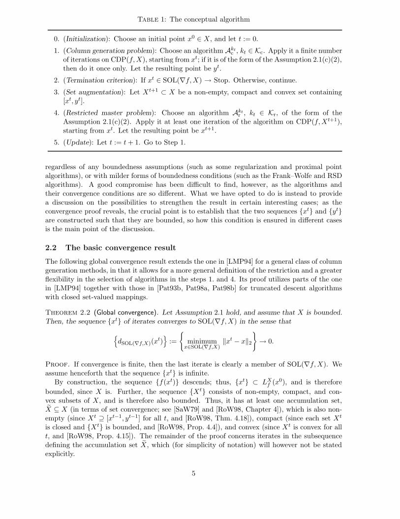
Table 1: The conceptual algorithm

0. (Initialization): Choose an initial point x0 ∈ X, and let t := 0.

1. (Column generation problem): Choose an algorithm Aktc , kt ∈ Kc. Apply it a finite number

of iterations on CDP(f,X), starting from xt; if it is of the form of the Assumption 2.1(c)(2),then do it once only. Let the resulting point be yt.

2. (Termination criterion): If xt ∈ SOL(∇f,X) → Stop. Otherwise, continue.

3. (Set augmentation): Let Xt+1 ⊂ X be a non-empty, compact and convex set containing[xt, yt].

4. (Restricted master problem): Choose an algorithm Aktr , kt ∈ Kr, of the form of the

Assumption 2.1(c)(2). Apply it at least one iteration of the algorithm on CDP(f,Xt+1),starting from xt. Let the resulting point be xt+1.

5. (Update): Let t := t+ 1. Go to Step 1.

regardless of any boundedness assumptions (such as some regularization and proximal pointalgorithms), or with milder forms of boundedness conditions (such as the Frank–Wolfe and RSDalgorithms). A good compromise has been difficult to find, however, as the algorithms andtheir convergence conditions are so different. What we have opted to do is instead to providea discussion on the possibilities to strengthen the result in certain interesting cases; as theconvergence proof reveals, the crucial point is to establish that the two sequences xt and ytare constructed such that they are bounded, so how this condition is ensured in different casesis the main point of the discussion.

2.2 The basic convergence result

The following global convergence result extends the one in [LMP94] for a general class of columngeneration methods, in that it allows for a more general definition of the restriction and a greaterflexibility in the selection of algorithms in the steps 1. and 4. Its proof utilizes parts of the onein [LMP94] together with those in [Pat93b, Pat98a, Pat98b] for truncated descent algorithmswith closed set-valued mappings.

Theorem 2.2 (Global convergence). Let Assumption 2.1 hold, and assume that X is bounded.Then, the sequence xt of iterates converges to SOL(∇f,X) in the sense that

dSOL(∇f,X)(x

t)

:=

minimum

x∈SOL(∇f,X)‖xt − x‖2

→ 0.

Proof. If convergence is finite, then the last iterate is clearly a member of SOL(∇f,X). Weassume henceforth that the sequence xt is infinite.

By construction, the sequence f(xt) descends; thus, xt ⊂ LXf (x0), and is therefore

bounded, since X is. Further, the sequence Xt consists of non-empty, compact, and con-vex subsets of X, and is therefore also bounded. Thus, it has at least one accumulation set,X ⊆ X (in terms of set convergence; see [SaW79] and [RoW98, Chapter 4]), which is also non-empty (since Xt ⊇ [xt−1, yt−1] for all t, and [RoW98, Thm. 4.18]), compact (since each set Xt

is closed and Xt is bounded, and [RoW98, Prop. 4.4]), and convex (since Xt is convex for allt, and [RoW98, Prop. 4.15]). The remainder of the proof concerns iterates in the subsequencedefining the accumulation set X, which (for simplicity of notation) will however not be statedexplicitly.

5

Since the number of iterations is infinite and the sets Kc and Kr are finite, there will be atleast one pair of elements in these sets, say (kc, kr), that appears an infinite number of times inthe subsequence defining the set X and in the same iterations as well. We henceforth considerthis further subsequence.

Since the sequence xt belongs to the compact set LXf (x0), it has a non-empty and bounded

set of accumulation points, say X ⊆ LXf (x0), which is closed (e.g., [Rud76, Thm. 3.7]). Since f is

continuous, we may find a convergent infinite subsequence, say xtt∈T , where T ⊆ 0, 1, 2, . . . ,with limit point xT ∈ arg max

x∈Xf(x). Further, xT ∈ X (e.g., [AuF90, Prop. 1.1.2]).

Denote by zt−1 ∈ Xt, t ∈ T , the first iterate of the algorithm Akr

r applied to the restrictedproblem CDP(f,Xt), starting from xt−1 ∈ Xt. Since each iteration of this algorithm givesdescent with respect to f , unless a stationary point to the RMP, CDP(f,Xt) is at hand, it followsthat, for all t ∈ T , f(xt) ≤ f(zt−1) < f(xt−1). Let xT −1 ∈ X be the limit point of a convergentinfinite subsequence of the sequence xt−1t∈T and let zT −1 ∈ X be an accumulation point ofthe corresponding subsequence of the sequence zt−1t∈T . Taking the limit corresponding tothis accumulation point, the continuity of f yields that f(xT ) ≤ f(zT −1) ≤ f(xT −1).

Since xT −1 ∈ X, the definition of xT implies that f(xT ) ≥ f(xT −1), and we conclude thatf(xT ) = f(zT −1) = f(xT −1). The latter equality together with the closedness and descentproperties of the iteration mapping of the algorithm Akr

r at non-stationary solutions gives thatxT −1 ∈ SOL(∇f, X). Then, from the relation f(xT ) = f(xT −1) and the definition of xT , weobtain that for all x ∈ X , f(x) ≥ f(xT ), and that for all x ∈ X, f(x) = f(xT ). Hence,X ⊆ SOL(∇f, X).

Now, let ε ≥ 0 be such that there is an infinite number of iterates xt−1 with dSOL(∇f,X)(xt−1) ≥

ε. This infinite subsequence of iterates has some accumulation point, say x, which is then thelimit point of some infinite convergent sequence xt−1

t∈T, where T ⊆ 0, 1, 2, . . . . From the

above we then know that x ∈ SOL(∇f, X).The sequence yt ⊆ X, and is therefore bounded.We first assume that the algorithm Akc

c is of type (c)(1). Let y be an arbitrary accumulationpoint of the subsequence yt−1

t∈T. Since yt−1 ∈ Xt for all t ∈ T , y ∈ X holds (e.g., [AuF90,

Prop. 1.1.2]). Since x ∈ SOL(∇f, X), we then have that ∇f(x)T(y − x) ≥ 0 holds. But if x /∈SOL(∇f,X) holds, then we obtain from the closedness and descent properties of the algorithmAkc

c that ∇f(x)T(y − x) < 0 holds, which yields a contradiction. Hence, x ∈ SOL (∇f,X).We next assume that the algorithm Akc

c is of type (c)(2). Since the sequence yt−1t∈T

⊆ X,

it has a non-empty, bounded and closed set of accumulation points, say Y . We define herein a

convergent infinite subsequence with limit point yT −1 ∈ arg maxy∈Y

f(y).

For all t ∈ T , let vt−1 ∈ X denote the point obtained by performing one iteration withthe algorithm Akc

c on the problem CDP(f,X), starting from xt−1. Since each iteration of thealgorithm Akc

c gives descent with respect to f , unless the current iterate is in SOL(∇f,X),it follows that, for all t ∈ T , f(yt−1) ≤ f(vt−1) < f(xt−1) < f(yt−2), where the latter strictinequality stems from the descent properties of the algorithm applied to the previous RMP.Taking the limit corresponding to the above defined subsequence, the continuity of f yields

that f(yT −1) ≤ f(x) ≤ f(vT −1) ≤ f(yT −2), where yT −2 denotes an accumulation point of thesequence yt−2

t∈T.

Since yT −2 ∈ Y , the definition of yT −1 implies that f(yT −1) ≥ f(yT −2), and we conclude

that f(yT −1) = f(vT −1) = f(x) = f(yT −2). The second equality together with the closednessand descent properties of the iteration mapping of the algorithm Akc

c at non-stationary solutionsgives that x ∈ SOL(∇f,X). [Moreover, Y ⊆ SOL(∇f,X).]

Hence, ε = 0.

6

The algorithmic mapping describing the algorithm identified by extracting the choices kc andkr from the collections Kc and Kr, and which defines the remaining iterates, is clearly of the formC(x) := y ∈ X | f(y) ≤ f(x) , x ∈ X , for any non-empty, compact and convex set X ⊆ X.We may therefore invoke the Spacer Step Theorem (e.g., [Lue84, p. 231]), which guarantees thatthe result holds for the whole sequence, thanks to the properties of the mappings given by thechoices kc and kr established above. This concludes the proof.

We note that although the algorithm, the above theorem and its proof concern stationarity,a version of the algorithm which uses only Assumption 2.1(c)(2) is valid also for other formsof “optimality”; simply replace “stationary” with “optimal” in the algorithm and the theorem.This observation also helps in tying together the algorithm with the convergence theorems A–D in Zangwill [Zan69, Pages 91, 128, 241, and 244]. Theorem A, as all the other theorems,presumes nothing about what the “solution” is, and presumes that the algorithm yields descentin each step outside the solution set with respect to a continuous merit function for the problem,and generates a bounded sequence. The other theorems relax some of these conditions slightly,and among other techniques, the spacer steps used in the above proof are introduced. Our needfor a special proof stems from two potential complications: the RMP is solved over a set whichmay vary rapidly between successive iterations, and in the column generation phase we allowfor two different solution principles.

2.3 Instances of the algorithm

These algorithms are analyzed mainly for the case where X is polyhedral.

Frank–Wolfe The vector yt is taken as any solution to the linearized problem

minimizey∈X

∇f(x)Ty; (2)

if, however, ∇f(xt)Td < 0 for some d in the recession cone of X, we let yt be defined such thatdt = yt − xt is a descent direction of unit length in the recession cone (such as the one obtainedin the simplex method when unboundedness is detected). The boundedness of xt and ytfollows from an assumption that the lower level set LX

f (x0) := X ∩ x ∈ ℜn | f(x) ≤ f(x0) is

bounded. We have that Xt := [xt, yt]; the RMP thus is a simple line search problem. Severalline search algorithms can be placed in the framework, including the exact line search mapping.

Simplicial decomposition The column generation problem is identical to that of the Frank–Wolfe algorithm. In the classic version, Xt+1 := conv (Xt∪yt), if no column dropping is used,or one first drops every column in Xt with zero weight in xt, if column dropping according tothe rule in [vHo77] is used. In both cases, clearly Xt+1 is a non-empty, compact and convexsubset of X, for which further Xt+1 ⊃ Xt holds for all t in the first case. [With reference to theabove convergence proof, if the sequence of restrictions is expanding, it is guaranteed to have aunique set limit (e.g., [SaW79])].

In the RSD version ([HLV87]), we let Xt+1 be given by the convex hull of xt and a finitenumber (at most r ∈ Z+) of the previously generated points ys, s = 1, 2, . . . , t, which alwaysincludes yt. (If r = 1 then the Frank–Wolfe algorithm is obtained.) More on RSD follows below.

The exact solution of the RMP can be viewed as a mapping of the form Aktr , which satisfies

the conditions of Assumption 2.1. In [HLV87], a truncated algorithm—the exact solution of thequadratic approximation of the RMP—is proposed and analyzed. Also this mapping is closed,has the fixed-point property, and provides descent under the conditions stated in that paper.

Later, we will establish that certain properties of SD are inherited by the general algorithm.For future reference, we therefore provide a few more details on the SD algorithm.

7

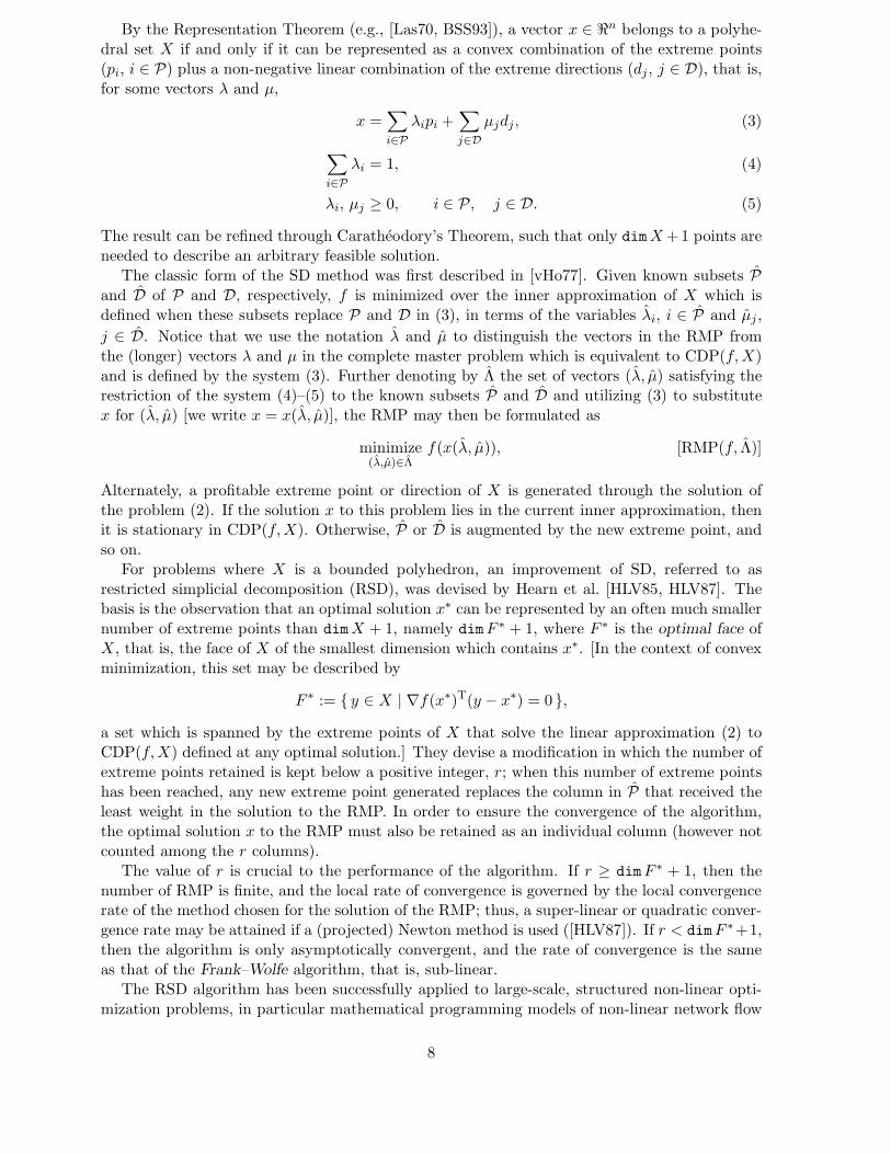
By the Representation Theorem (e.g., [Las70, BSS93]), a vector x ∈ ℜn belongs to a polyhe-dral set X if and only if it can be represented as a convex combination of the extreme points(pi, i ∈ P) plus a non-negative linear combination of the extreme directions (dj , j ∈ D), that is,for some vectors λ and µ,

x =∑

i∈P

λipi +∑

j∈D

µjdj, (3)

∑

i∈P

λi = 1, (4)

λi, µj ≥ 0, i ∈ P, j ∈ D. (5)

The result can be refined through Caratheodory’s Theorem, such that only dimX+1 points areneeded to describe an arbitrary feasible solution.

The classic form of the SD method was first described in [vHo77]. Given known subsets Pand D of P and D, respectively, f is minimized over the inner approximation of X which isdefined when these subsets replace P and D in (3), in terms of the variables λi, i ∈ P and µj ,

j ∈ D. Notice that we use the notation λ and µ to distinguish the vectors in the RMP fromthe (longer) vectors λ and µ in the complete master problem which is equivalent to CDP(f,X)and is defined by the system (3). Further denoting by Λ the set of vectors (λ, µ) satisfying therestriction of the system (4)–(5) to the known subsets P and D and utilizing (3) to substitutex for (λ, µ) [we write x = x(λ, µ)], the RMP may then be formulated as

minimize(λ,µ)∈Λ

f(x(λ, µ)), [RMP(f, Λ)]

Alternately, a profitable extreme point or direction of X is generated through the solution ofthe problem (2). If the solution x to this problem lies in the current inner approximation, thenit is stationary in CDP(f,X). Otherwise, P or D is augmented by the new extreme point, andso on.

For problems where X is a bounded polyhedron, an improvement of SD, referred to asrestricted simplicial decomposition (RSD), was devised by Hearn et al. [HLV85, HLV87]. Thebasis is the observation that an optimal solution x∗ can be represented by an often much smallernumber of extreme points than dimX + 1, namely dimF ∗ + 1, where F ∗ is the optimal face ofX, that is, the face of X of the smallest dimension which contains x∗. [In the context of convexminimization, this set may be described by

F ∗ := y ∈ X | ∇f(x∗)T(y − x∗) = 0 ,

a set which is spanned by the extreme points of X that solve the linear approximation (2) toCDP(f,X) defined at any optimal solution.] They devise a modification in which the number ofextreme points retained is kept below a positive integer, r; when this number of extreme pointshas been reached, any new extreme point generated replaces the column in P that received theleast weight in the solution to the RMP. In order to ensure the convergence of the algorithm,the optimal solution x to the RMP must also be retained as an individual column (however notcounted among the r columns).

The value of r is crucial to the performance of the algorithm. If r ≥ dimF ∗ + 1, then thenumber of RMP is finite, and the local rate of convergence is governed by the local convergencerate of the method chosen for the solution of the RMP; thus, a super-linear or quadratic conver-gence rate may be attained if a (projected) Newton method is used ([HLV87]). If r < dimF ∗+1,then the algorithm is only asymptotically convergent, and the rate of convergence is the sameas that of the Frank–Wolfe algorithm, that is, sub-linear.

The RSD algorithm has been successfully applied to large-scale, structured non-linear opti-mization problems, in particular mathematical programming models of non-linear network flow

8

problems, where the column generation subproblem reduces to efficiently solvable linear net-work flow problems (e.g., [HLV87, LaP92]). Experience with the RSD method has shown thatit makes rapid progress initially, especially when relatively large values of r are used and whensecond-order methods are used for the solution of the RMP, but that it slows down close to anoptimal solution. It is also relatively less efficient for larger values of dimF ∗, since the numberand size of the RMP solved within the method become larger.

The explanation for this behaviour is to be found in the construction of a linear columngeneration subproblem: the quality of the resulting search directions is known to deterioraterapidly. (As the sequence xt tends to a stationary point, the sequence ∇f(xt)Tdt of di-rectional derivatives of the search directions dt := yt − xt tends to zero whereas dt does not;thus, the search directions rapidly tend to become nearly orthogonal to the gradient of f .) Sim-ilarly, the quality of the columns generated in this fashion will also deteriorate in terms of theirimprovement in the objective value. It is a natural conclusion that better approximations of fcan be exploited in the column generation phase of SD methods; then, the columns generatedwould be of better quality, thus leading to larger improvements in the inner approximations ofthe feasible set.

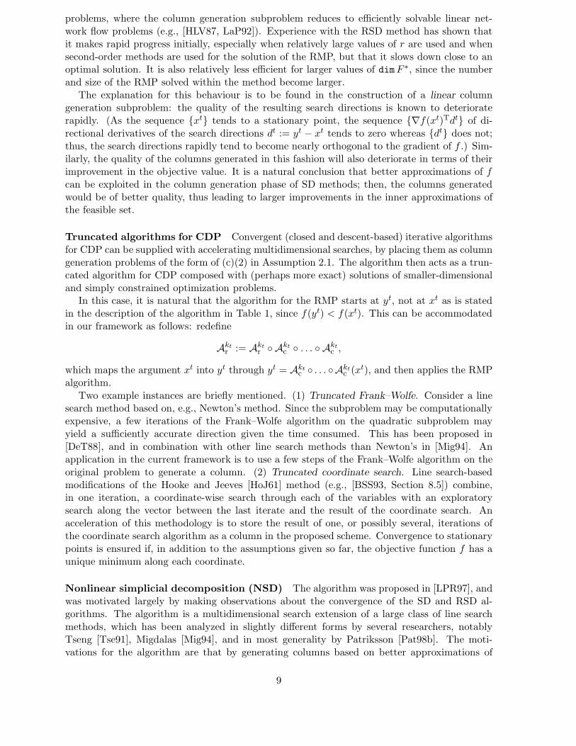
Truncated algorithms for CDP Convergent (closed and descent-based) iterative algorithmsfor CDP can be supplied with accelerating multidimensional searches, by placing them as columngeneration problems of the form of (c)(2) in Assumption 2.1. The algorithm then acts as a trun-cated algorithm for CDP composed with (perhaps more exact) solutions of smaller-dimensionaland simply constrained optimization problems.

In this case, it is natural that the algorithm for the RMP starts at yt, not at xt as is statedin the description of the algorithm in Table 1, since f(yt) < f(xt). This can be accommodatedin our framework as follows: redefine

Aktr := Akt

r Aktc . . . Akt

c ,

which maps the argument xt into yt through yt = Aktc . . . Akt

c (xt), and then applies the RMPalgorithm.

Two example instances are briefly mentioned. (1) Truncated Frank–Wolfe. Consider a linesearch method based on, e.g., Newton’s method. Since the subproblem may be computationallyexpensive, a few iterations of the Frank–Wolfe algorithm on the quadratic subproblem mayyield a sufficiently accurate direction given the time consumed. This has been proposed in[DeT88], and in combination with other line search methods than Newton’s in [Mig94]. Anapplication in the current framework is to use a few steps of the Frank–Wolfe algorithm on theoriginal problem to generate a column. (2) Truncated coordinate search. Line search-basedmodifications of the Hooke and Jeeves [HoJ61] method (e.g., [BSS93, Section 8.5]) combine,in one iteration, a coordinate-wise search through each of the variables with an exploratorysearch along the vector between the last iterate and the result of the coordinate search. Anacceleration of this methodology is to store the result of one, or possibly several, iterations ofthe coordinate search algorithm as a column in the proposed scheme. Convergence to stationarypoints is ensured if, in addition to the assumptions given so far, the objective function f has aunique minimum along each coordinate.

Nonlinear simplicial decomposition (NSD) The algorithm was proposed in [LPR97], andwas motivated largely by making observations about the convergence of the SD and RSD al-gorithms. The algorithm is a multidimensional search extension of a large class of line searchmethods, which has been analyzed in slightly different forms by several researchers, notablyTseng [Tse91], Migdalas [Mig94], and in most generality by Patriksson [Pat98b]. The moti-vations for the algorithm are that by generating columns based on better approximations of

9

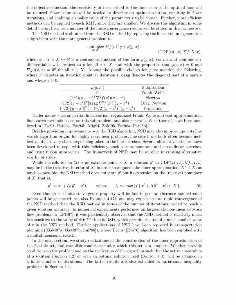
the objective function, the sensitivity of the method to the dimension of the optimal face willbe reduced, fewer columns will be needed to describe an optimal solution, resulting in feweriterations, and enabling a smaller value of the parameter r to be chosen. Further, more efficientmethods can be applied to each RMP, since they are smaller. We discuss this algorithm in somedetail below, because a number of the finite convergence results will be stated in this framework.

The NSD method is obtained from the RSD method by replacing the linear column generationsubproblem with the more general problem to

minimizey∈X

∇f(x)Ty + ϕ(y, x),[CDP(ϕ(·, x),∇f,X, x)]

where ϕ : X × X 7→ ℜ is a continuous function of the form ϕ(y, x), convex and continuouslydifferentiable with respect to y for all x ∈ X, and with the properties that ϕ(x, x) = 0 and∇yϕ(x, x) = 0n for all x ∈ X. Among the possible choices for ϕ we mention the following,where xt denotes an iteration point at iteration t, diag denotes the diagonal part of a matrixand where γ > 0:

ϕ(y, xt) Subproblem

0 Frank–Wolfe(1/2)(y − xt)T∇2f(xt)(y − xt) Newton

(1/2)(y − xt)T[diag∇2f(xt)](y − xt) Diag. Newton(γ/2)‖y − xt‖2 := (γ/2)(y − xt)T(y − xt) Projection

Under names such as partial linearization, regularized Frank–Wolfe and cost approximation,line search methods based on this subproblem, and also generalizations thereof, have been ana-lyzed in [Tse91, Pat93a, Pat93b, Mig94, ZhM95, Pat98a, Pat98b].

Besides providing improvements over the RSD algorithm, NSD may also improve upon its linesearch algorithm origin; for highly non-linear problems, line search methods often become inef-fective, due to very short steps being taken in the line searches. Several alternative schemes havebeen developed to cope with this deficiency, such as non-monotone and curve-linear searches,and trust region approaches. The framework of NSD may be another interesting alternativeworthy of study.

While the solution to (2) is an extreme point of X, a solution yt to CDP(ϕ(·, x),∇f,X, x)may be in the (relative) interior of X; in order to augment the inner approximation, Xt ⊂ X, asmuch as possible, the NSD method does not store yt but its extension on the (relative) boundaryof X, that is,

yt := xt + ℓt(yt − xt), where ℓt := max ℓ | xt + ℓ(yt − xt) ∈ X . (6)

Even though the finite convergence property will be lost in general (because non-extremalpoints will be generated, see also Example 4.17), one may expect a more rapid convergence ofthe NSD method than the RSD method in terms of the number of iterations needed to reach agiven solution accuracy. In numerical experiments performed on large-scale non-linear networkflow problems in [LPR97], it was particularly observed that the NSD method is relatively muchless sensitive to the value of dimF ∗ than is RSD, which permits the use of a much smaller valueof r in the NSD method. Further applications of NSD have been reported in transportationplanning ([GaM97a, GaM97b, LuP98]), where Evans’ [Eva76] algorithm has been supplied witha multidimensional search.

In the next section, we study realizations of the construction of the inner approximation ofthe feasible set, and establish conditions under which this set is a simplex. We then provideconditions on the problem and on the realization of the algorithm such that the active constraintsat a solution (Section 4.2) or even an optimal solution itself (Section 4.3), will be attained ina finite number of iterations. The latter results are also extended to variational inequalityproblems in Section 4.4.

10

3 Properties of the RMP

As has been remarked upon in Section 2, the inner approximations of the set X employed in SDmethods are polyhedral sets whose extreme points are extreme points of X. In RSD, the innerapproximation is slightly redefined such that whenever a column dropping has been performed,the previous solution to the RMP is also retained as a column.

One may consider more general rules for constructing the inner approximation; cf., for exam-ple, the condition on Xt+1 in Step 3 in the description of the conceptual algorithm in Table 1. Inorder to establish properties similar to those for SD methods, it is necessary to introduce furtherconditions on the updating of the sets Xt. In this section, we establish rules for introducing anddropping columns so as to maintain the simplicial property of the sets Xt.

3.1 Set augmentation

When determining the updating of the inner approximation from one iteration to the next, weconsider two phases.

First, given the solution xt to the current RMP, we may drop columns from the active set,for example based on their barycentric coordinates (weights) in describing xt. If we employ arestriction strategy corresponding to that of Hearn et al. [HLV85, HLV87] based on a maximumnumber of columns stored, we may also drop columns that have more than an insignificantweight, while then also introducing the vector xt as an individual column.

Second, a main difference between the simplicial decomposition method, as proposed byvon Hohenbalken and successors, and the method of this paper, is that the columns are notnecessarily extreme points of X. We however do assume that the columns introduced belong tothe (relative) boundary of X. This corresponds to utilizing, if necessary, the rule (6).

In the following, we use Pts to denote the set of columns generated in Step 1 of the CG

algorithm, and retained at iteration t; further, Ptx is either an empty set or it contains one

column which corresponds to the result of Step 4 in the previous iteration.Table 2 summarizes the various rules considered in the introduction of new and deletion

of old columns; they are realizations of Step 3 in the conceptual algorithm of Table 1. (Thecorresponding initializations necessary are also included.)

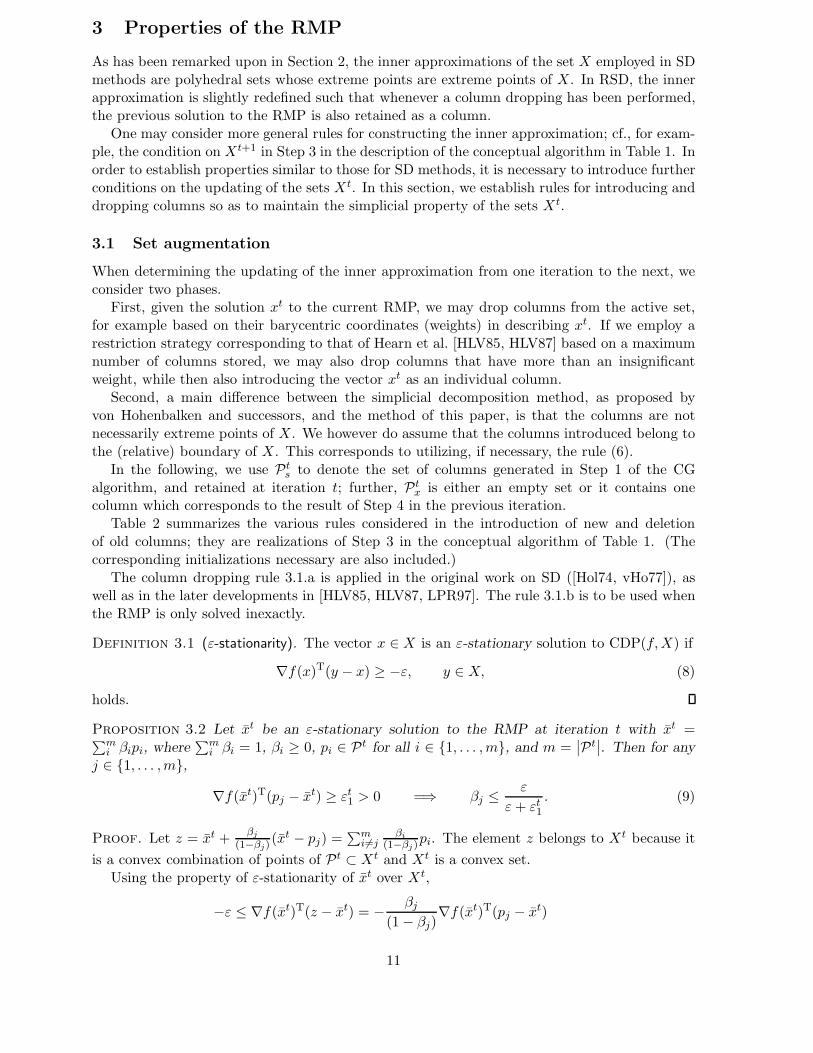
The column dropping rule 3.1.a is applied in the original work on SD ([Hol74, vHo77]), aswell as in the later developments in [HLV85, HLV87, LPR97]. The rule 3.1.b is to be used whenthe RMP is only solved inexactly.

Definition 3.1 (ε-stationarity). The vector x ∈ X is an ε-stationary solution to CDP(f,X) if

∇f(x)T(y − x) ≥ −ε, y ∈ X, (8)

holds.

Proposition 3.2 Let xt be an ε-stationary solution to the RMP at iteration t with xt =∑mi βipi, where

∑mi βi = 1, βi ≥ 0, pi ∈ Pt for all i ∈ 1, . . . ,m, and m =

∣∣Pt∣∣. Then for any

j ∈ 1, . . . ,m,

∇f(xt)T(pj − xt) ≥ εt1 > 0 =⇒ βj ≤ε

ε+ εt1. (9)

Proof. Let z = xt +βj

(1−βj)(xt − pj) =

∑mi6=j

βi

(1−βj)pi. The element z belongs to Xt because it

is a convex combination of points of Pt ⊂ Xt and Xt is a convex set.Using the property of ε-stationarity of xt over Xt,

−ε ≤ ∇f(xt)T(z − xt) = −βj

(1 − βj)∇f(xt)T(pj − xt)

11

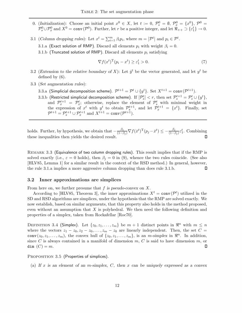
Table 2: The set augmentation phase

0. (Initialization): Choose an initial point x0 ∈ X, let t := 0, P0s = ∅, P0

x = x0, P0 =P0

s ∪P0x and X0 = conv (P0). Further, let r be a positive integer, and let ℜ++ ⊃ εt1 → 0.

3.1 (Column dropping rules): Let xt =∑m

i=1 βipi, where m =∣∣Pt

∣∣ and pi ∈ Pt.

3.1.a (Exact solution of RMP). Discard all elements pi with weight βi = 0.

3.1.b (Truncated solution of RMP). Discard all elements pi satisfying

∇f(xt)T(pi − xt) ≥ εt1 > 0. (7)

3.2 (Extension to the relative boundary of X): Let yt be the vector generated, and let yt bedefined by (6).

3.3 (Set augmentation rules):

3.3.a (Simplicial decomposition scheme). Pt+1 = Pt ∪ yt. Set Xt+1 = conv(Pt+1).

3.3.b (Restricted simplicial decomposition scheme). If∣∣Pt

s

∣∣ < r, then set Pt+1s = Pt

s ∪ yt,and Pt+1

x = Ptx; otherwise, replace the element of Pt

s with minimal weight inthe expression of xt with yt to obtain Pt+1

s , and let Pt+1x = xt. Finally, set

Pt+1 = Pt+1s ∪ Pt+1

x and Xt+1 = conv (Pt+1).

holds. Further, by hypothesis, we obtain that −βj

(1−βj)∇f(xt)T(pj− x

t) ≤ −βj

(1−βj)εt1. Combining

these inequalities then yields the desired result.

Remark 3.3 (Equivalence of two column dropping rules). This result implies that if the RMP issolved exactly (i.e., ε = 0 holds), then βj = 0 in (9), whence the two rules coincide. (See also[HLV85, Lemma 1] for a similar result in the context of the RSD method.) In general, however,the rule 3.1.a implies a more aggressive column dropping than does rule 3.1.b.

3.2 Inner approximations are simplices

From here on, we further presume that f is pseudo-convex on X.According to [HLV85, Theorem 3], the inner approximations Xt = conv (Pt) utilized in the

SD and RSD algorithms are simplices, under the hypothesis that the RMP are solved exactly. Wenow establish, based on similar arguments, that this property also holds in the method proposed,even without an assumption that X is polyhedral. We then need the following definition andproperties of a simplex, taken from Rockafellar [Roc70].

Definition 3.4 (Simplex). Let z0, z1, . . . , zm be m + 1 distinct points in ℜn with m ≤ nwhere the vectors z1 − z0, z2 − z0, . . . , zm − z0 are linearly independent. Then, the set C =conv (z0, z1, . . . , zm), the convex hull of z0, z1, . . . , zm, is an m-simplex in ℜn. In addition,since C is always contained in a manifold of dimension m, C is said to have dimension m, ordim (C) = m.

Proposition 3.5 (Properties of simplices).

(a) If x is an element of an m-simplex, C, then x can be uniquely expressed as a convex

12

combination of points, z0, z1, . . . , zm, defining C, i.e.,

x =m∑

i=0

βizi,m∑

i=0

βi = 1, βi ≥ 0, i = 0, 1, . . . ,m,

and β0, β1, . . . , βm are unique.

(b) If x is an element of an m-simplex, C, and the convexity weight, βi, for some i = 0, 1, . . . ,mis positive in the (unique) expression of x as a convex combination of z0, z1, . . . , zm, thenthe set conv (z0, z1, . . . , zi−1, x, zi+1, . . . , zm) is an m-simplex.

(c) If conv (z0, z1, . . . , zm) is an m-simplex, then conv (z0, z1, . . . , zi−1, zi+1, . . . , zm), for somei = 0, 1, . . . ,m, is an (m− 1)-simplex.

The main result of this section follows.

Theorem 3.6 (The inner approximation is a simplex). Assume that the RMP are solved exactly.Then, the set Xt is a simplex for all t.

Proof. We show by induction that Xt is a simplex at the start of Step 3.3. It follows that Xt

is a simplex in every step of the algorithm.When t = 0, Xt = x0; therefore, X0 is a 0-simplex. Assume now that Xt is a simplex for

t ≥ 0. The elements with zero weight have been discarded at the beginning of Step 3.3; therefore,the remaining elements in Pt must have positive weight. By the induction hypothesis andProposition 3.5.c the points not eliminated define a simplex. Assume without loss of generalitythat at the beginning of Step 3.3, Pt = p0, p1, . . . , pm, and that, by assumption, Pt defines anm-simplex. We denote the convex hull of this set by Xt.

The element xt is expressed as

xt =m∑

i=0

βipi, with βi > 0 and pi ∈ Pt.

It follows that xt ∈ rint (Xt). We will prove that if xt is not an optimal solution to [CDP(f,X)]then conv (Xt∪yt) is a simplex, where yt is the column added in iteration t+1. First, however,we note that xt is also an optimal solution to the problem of minimizing f over aff (Xt) ∩X,where aff (Xt) is the affine hull of Xt, since no constraint of the form βi ≥ 0 is binding, so

∇f(xt)T(y − xt) ≥ 0, y ∈ aff (Xt) ∩X, (10)

which we proceed to establish.Let y be an arbitrary element of aff (Xt) ∩ X. If y ∈ Xt ⊂ Xt then the point y satisfies

the inequality in (10) because xt solves the RMP over Xt. Otherwise, y ∈ aff (Xt) − Xt.Using the fact that xt is in the relative interior of Xt, there exists a unique element, z, inthe set [xt, y] ∩ rfro (Xt), where rfro(Xt) is the relative boundary of Xt. This point satisfiesy = xt +λ(z−xt) for some λ > 1. By the optimality of xt over Xt and the fact that z ∈ Xt, weobtain that ∇f(xt)T(z−xt) ≥ 0, whence it follows that ∇f(xt)T(y−xt) = λ[∇f(xt)T(z−xt)] ≥ 0.This completes the proof of (10).

If xt solves [CDP(f,X)] then the algorithm terminates without generating Xt+1. Otherwise,by Assumption 2.1.c and the use of the rule (6), it follows that the column yt generated inStep 3.2 satisfies ∇f(xt)T(yt − xt) < 0. This relation, together with the optimality of xt overaff (Xt) ∩X, implies that yt /∈ aff (Xt). As Xt is an m-simplex by the induction hypothesis,conv (Xt ∪ yt) is therefore an (m+ 1)-simplex.

In the case that m =∣∣Pt

s

∣∣ < r holds, that set is produced by Step 3.3.a and Step 3.3.b.The only other case to consider is the use of Step 3.3.b in the case when m =

∣∣Pts

∣∣ = r

13

holds. We will then assume without loss of generality that Pts = p0, . . . , pm−1, and let

Ptx = x′. By assumption, Pt defines an m-simplex. In this case Xt+1 = conv (Pt+1) where

Pt+1 = p0, . . . , pi−1, pi+1, . . . , pm−1, xt, yt, for some i. This set defines an m-simplex be-

cause conv (p0, p1, . . . , pm−1, x′, yt) is an (m + 1)-simplex by the above, by Proposition 3.5.b

(p0, p1, . . . , pm−1, xt, yt) is an (m + 1)-simplex, and conv (p0, . . . , pi−1, pi+1, . . . , pm−1, x

t, yt) =:Xt+1 is an m-simplex by Proposition 3.5.c. Thus, in either case, conv (Pt+1) is a simplex. Thiscompletes the proof.

4 Finiteness convergence properties of the column generation

algorithm

This section offers some insight into the finite convergence properties of the column generationalgorithm proposed. The investigation is divided in two parts. First, we establish conditions onthe problem and on the algorithm so that the optimal face will be attained in a finite numberof iterations. When X is polyhedral, this result implies the finite identification of the activeconstraints at the limit point. Second, we study the stronger property of finitely attaining anoptimal solution, under the condition of weak sharpness of the set SOL(f,X). We finally extendthese results to variational inequality problems.

4.1 Facial geometry and non-degeneracy

We begin with some elementary properties of faces of convex sets.

Definition 4.1 (Face). Let X be a convex set in ℜn. A convex set F is a face of X if theendpoints of any closed line segment in X whose relative interior intersects F are contained inF . Thus, if x and y are in X and λx+ (1−λ)y lies in F for some 0 < λ < 1, then x and y mustalso belong to F .

The following two results appear in [Roc70, Theorems 18.1–2].

Theorem 4.2 Let F be a face of the convex set X. If Ω is a convex subset of X so that rintΩmeets F , then Ω ⊂ F .

A corollary to this result is that if the relative interiors of two faces F1 and F2 have anon-empty intersection then they are equal. The following result complements the above byestablishing that each point in a convex set belongs to the relative interior of a unique face.

Theorem 4.3 The collection of all relative interiors of faces of the convex set X is a partitionof X.

We will use the notation F (x) to denote the unique face F of X for which x ∈ rintF . Notethat this is the minimal face containing the point x. We will subsequently characterize theseminimal faces.

Definition 4.4 (The k-tangent cone KX(x)). A vector v is said to be k-tangent to the set X atthe point x in X if for some ε > 0, x+ tv ∈ X holds for all t ∈ (−ε, ε). The set of all k-tangentvectors v at x is a cone, which we denote by KX(x).

For any cone C, let linC denote the lineality of C, the largest subspace contained in C, thatis, linC = C ∩ (−C).

14

Lemma 4.5 (Characterization of F (x)). Let x ∈ X. It holds that F (x) = (x+ linKX(x)) ∩X.

Proof. It is obvious that (x + linKX(x)) ∩ X is a face of X satisfying x ∈ rint ((x +linKX(x)) ∩X) ∩ rintF (x). Using Theorem 4.3 these faces are identical.

Recall next the definition (1) of the normal cone NX(x) to the set X at x. We note thatif F is a face of X, then the normal cone is independent of x ∈ rintF , whence we may writeNX(F ). The tangent cone to X at x, TX(x), is the polar cone of NX(x). The face of X exposedby the vector d ∈ ℜn (the exposed face) is the set

EX(d) = arg maxy∈X

dTy.

For general convex sets, x ∈ EX(d) holds if and only if d ∈ NX(x) (e.g., [BuM94]), whereasfor polyhedral sets, the exposed face is independent of the choice of d ∈ rintNX(x). Further,every face of a polyhedral set is exposed by some vector d. These results however fail to holdfor general convex sets. In the analysis of identification properties of the CG algorithm, we willfocus on faces of X which enjoy stronger properties than faces in general.

Definition 4.6 (Quasi-polyhedral face). A face F of X is quasi-polyhedral if

affF = x+ linTX(x), x ∈ rintF. (11)

The relative interior of a quasi-polyhedral face is equivalent to an open facet, as defined in[Dun87]. Every face of a polyhedral set X is quasi-polyhedral, but this is not true for a generalconvex set, as the example in [BuM88] shows. Further, a quasi-polyhedral face need not to bea polyhedral set, and vice versa. Quasi-polyhedral faces are however exposed by any vector inrintNX(F ), and have several other properties in common with faces of polyhedral sets. See[BuM88, BuM94] for further properties of quasi-polyhedral faces.

We now turn to study the optimal face of X. The following definition extends the classic onefor problems with unique solutions (e.g., [Wol70]).

Definition 4.7 (Optimal face). The optimal face of [CDP(f,X)] is

F ∗ =⋂

x∗∈SOL(f,X)

Fx∗ ,

where Fx∗ = y ∈ X | ∇f(x∗)T(y − x∗) = 0 .

The set F ∗ is a face because it is the intersection of a collection of faces. It is elementaryto show that whenever f is pseudo-convex, F ∗ ⊃ SOL(f,X) holds. Further note that for anystationary point x∗, the face Fx∗ is the exposed face EX(−∇f(x∗)).

In the case where f is convex, we recall that the value of ∇f is constant on SOL(f,X), by aresult of Burke and Ferris [BuF91]. Therefore, in this case, F ∗ = Fx∗ = EX(−∇f(x∗)) for anyx∗ ∈ SOL(f,X), simplifying the above definition.

Under the following regularity condition on an optimal solution, the finite identification ofthe optimal face has been demonstrated for several algorithms (e.g., [Dun87, BuM88, Pat98b]):

Definition 4.8 (Non-degenerate solution). An optimal solution x∗ to [CDP(f,X)] is non-degenerate if

−∇f(x∗) ∈ rintNX(x∗) (12)

holds.

15

We note that this regularity condition does not depend on the representation of the set X.When X is described explicitly with constraints, then the condition is weaker than strict comple-mentarity ([BuM88]). Before establishing the finite identification result for the CG algorithm,we introduce two other regularity conditions that have been used in the literature, and relatethem to each other.

Definition 4.9 (Conditions of regularity). (1) (Geometric stability, [MaD89]). An optimal solu-tion x∗ is geometrically stable if

∇f(x∗)T(x− x∗) = 0 =⇒ x ∈ F ∗. (13)

(2) (Geometric regularity, [DuM89]). The optimal face F ∗ is geometrically regular if

SOL(f,X) ⊂ rintF ∗, (14)

and the set SOL(f,X) is non-degenerate in the sense of Definition 4.8.

A sufficient condition for geometric stability is the convexity of f on X, as remarked above.The notions of geometric stability and regularity are equivalent when X is a bounded polyhe-

dral set (see [DuM89, Corollary 2.4]). The following result extends this characterization to thecase of general convex sets under a non-degeneracy assumption. (The constraint qualification(CQ) of Guignard [Gui69] utilized in the result implies that NX(x) is a polyhedral cone for everyx, and is satisfied automatically for polyhedral sets X.)

Theorem 4.10 (Relations among conditions of regularity). Assume that Guignard’s CQ holds.Further, assume that SOL(f,X) is a set of non-degenerate optimal solutions. Consider thefollowing three statements.

(a) F ∗ is geometrically regular.

(b) F ∗ is a quasi-polyhedral face, and F ∗ = F (x∗) holds for all x∗ ∈ SOL(f,X).

(c) Every x∗ ∈ SOL(f,X) is geometrically stable.

It then holds that (a) =⇒ (b) =⇒ (c).

Proof. [(a) =⇒ (b)]. The following relationship holds: x∗ ∈ (rintF ∗) ∩ (rintF (x∗)) for allx∗ ∈ SOL(f,X) . By Theorem 4.3, F ∗ = F (x∗) holds for all x∗ ∈ SOL(f,X) .

We now prove that F ∗ is a quasi-polyhedral face. As x∗ ∈ rintF ∗, we demonstrate that F ∗ =(x∗ + lin (TX(x∗))∩X. We begin by showing that F ∗ ⊂ (x∗ + lin (TX(x∗))∩X. Using Lemma4.5, we obtain that F ∗ = (x∗ +KX(x∗)) ∩ X. Moreover, KX(x∗) ⊂ TX(x∗) and linKX(x) =KX(x), which establishes the inclusion. Conversely, let x∗ + v ∈ (x∗ + lin (TX(x∗)) ∩ X. UsingLemma 2.7 in [BuM88], it follows that v ∈ N⊥

X (x∗), where ⊥ denotes the orthogonal complement.On the other hand, N⊥

X (x∗) = N⊥X (z) holds for all z ∈ rintF ∗ (see [BuM88, Theorem 2.3]).

This implies that v ∈ N⊥X (y∗) for every y∗ ∈ SOL(f,X) . As −∇f(y∗) ∈ NX(y∗), ∇f(y∗)Tv = 0

holds for every y∗ ∈ SOL(f,X) . This relationship establishes that ∇f(y∗)T(x∗ + v − y∗) =∇f(y∗)Tv + ∇f(y∗)T(x∗ − y∗) = 0, and x∗ + v ∈ Fy∗ for all y∗ ∈ SOL(f,X) . By the definitionof F ∗, we obtain that x∗ + v ∈ F ∗.

[(b) =⇒ (c)]. Let x∗ ∈ SOL(f,X) . We prove that if ∇f(x∗)T(z − x∗) = 0, for z ∈ X,then z ∈ F ∗. As NX(x∗) is a polyhedral cone and −∇f(x∗) ∈ NX(x∗), a set of vectors andscalars exists so that −∇f(x∗) =

∑λivi, where λi ≥ 0. The point x∗ is non-degenerate;

using Lemma 3.2 of [BuM88] these coefficients must therefore be positive. The relationship0 = −∇f(x∗)T(z − x∗) =

∑λiv

Ti (z − x∗) implies that vT

i (z − x∗) = 0 for all i, and hencethat (z − x∗) ∈ N⊥

X (x∗). Using Lemma 2.7 of [BuM88], N⊥X (x∗) = linTX(x∗). By hypothesis,

16

F ∗ = (x∗ + lin (TX(x∗)) ∩ X and z = x∗ + (z − x∗) ∈ (x∗ + lin (TX(x∗)) ∩ X = F ∗. Thiscompletes the proof.

The result can not be strengthened to an equivalence among all three: (c) =⇒ (a) may failfor non-polyhedral sets.

4.2 Finite identification of the optimal face

The identification results to follow will be established under the following assumption on theconstruction and solution of the sequence of RMP:

Assumption 4.11 (Conditions on the RMP). Either one of the following conditions hold.

(1) r ≥ dimF ∗ + 1, and the RMP are solved exactly.

(2) r = ∞, and the RMP are solved such that xt is εt-optimal with εt ↓ 0.

Theorem 4.12 (Identification results). Let xt and yt be the sequence of iterates andcolumns generated by the algorithm, and assume that xt converges to x∗ ∈ SOL(f,X).

(a) Assume further that the RMP are solved exactly. If a positive integer τ1 exists such thatxt ∈ rintF ∗ for every t ≥ τ1, then there exists a positive integer τ2 such that

yt ∈ F ∗, t ≥ τ2.

(b) Let Assumption 4.11 hold, and assume that F ∗ is geometrically regular. If a positiveinteger τ1 exists such that yt ∈ F ∗ for every t ≥ τ1, then there exists a positive integer τ2such that

xt ∈ rintF ∗, t ≥ τ2.

Proof. (a) Let t ≥ τ1, so that xt ∈ rintF ∗. First we show that the column yt+1 generated bythe rule (6) belongs to the optimal face F ∗. Since in each iteration the RMP is solved exactly,xt+1 ∈ Xt+1 − Xt holds, and hence xt+1 = λyt+1 + (1 − λ)z, where z ∈ Xt and 0 < λ ≤ 1.If λ = 1 then the result follows trivially. Otherwise, using the fact that F ∗ is a face, and thatxt+1 ∈ (z, yt+1) ∩ rintF ∗, we have that [z, yt+1] ⊂ F ∗, and hence yt+1 belongs to the optimalface. Now we show that also yt+1 belongs to F ∗. Using that xt+1 ∈ rintF ∗ ⊂ F ∗, it followsthat [xt+1, yt+1] ⊂ F ∗. Since yt+1 ∈ [xt+1, yt+1] holds, the result follows.

(b) Let t ≥ τ1, so that yt ∈ F ∗. If yt ∈ rintF ∗, then since F ∗ is a face of X, also yt belongsto F ∗. Otherwise, yt ∈ rfroF ∗, whence the rule (6) produces yt = yt ∈ F ∗. This guaranteesthat ytt≥τ1 ⊂ F ∗.

We next prove that if there exists an element z that is never discarded from the set Pt fort ≥ τ , then z is in the optimal face. This is obviously possible if and only if z does not satisfythe column dropping rule in any iteration t ≥ τ . Let t ≥ τ , and let the solution to the RMP atiteration t be expressed by

xt+1 = βtzz +

nt∑

i=1

βtipi, 0 < βt

z, 0 ≤ βti , i = 1, . . . , nt and βt

z +nt∑

i=1

βti = 1, pi ∈ Pt.

If the RMP is solved inexactly, then the fact that z does not satisfy the column dropping ruleimplies that ∇f(xt+1)T(z − xt+1) < εt+1

1 . Using the continuity of ∇f(x), and taking the limitof the inequality, we obtain that

∇f(x∗)T(z − x∗) = limt→∞

∇f(xt+1)T(z − xt+1) ≤ limt→∞

εt1 = 0.

17

By the optimality of x∗, we obtain that ∇f(x∗)T(z − x∗) ≥ 0, which implies that ∇f(x∗)T(z −x∗) = 0. If however the RMP is solved exactly, then ∇f(xt+1)T(z−xt+1) = 0 must hold, becauseotherwise it would have to be positive by the optimality of xt+1, which in turn would imply byProposition 3.2 that βt

z = 0; this however contradicts our assumption that βtz > 0. In the limit

of the above equality, then,

∇f(x∗)T(z − x∗) = limt→∞

∇f(xt+1)T(z − xt+1) = 0.

Since x∗ is geometrically stable, in either case we have established that z ∈ F ∗.This also proves that any element of the set ∪t>τP

t which is not in the optimal face mustbe eliminated in some iteration. We first consider the case where r = ∞ holds. By the above,yt ∈ F ∗ for t ≥ τ1. Hence, by the construction of the inner approximation, there exists aninteger τ2 such that Pt ⊂ F ∗, for t ≥ τ2. We therefore obtain that xt ∈ Xt = conv(Pt) ⊂ F ∗,t ≥ τ2. The fact that the weights are positive then implies that actually xt ∈ rintF ∗.

In the case where r < ∞, it may be that there are iterations t in which an element xt isintroduced into Pt. We however establish that this is impossible when r ≥ dimF ∗ + 1 and theRMP are solved exactly. The conclusion is then the same as for the case when r = ∞.

Using the previous result, Pts ⊂ F ∗ for all t ≥ τ2. This implies that dim (conv (Pt

s)) ≤ dimF ∗.For future reference, let dim (conv (Pt

s)) = m. As the RMP are solved exactly, Xt is a simplexby Theorem 3.6 for any t ≥ 0, so conv (Pt

s) is an m-simplex by Proposition 3.5.c. Consider thecolumn yt generated for some iteration t ≥ τ2. Since we assume that xt /∈ SOL(f,X), accordingto the proof of Theorem 3.6, conv (Pt

s ∪ yt) is then an (m+ 1)-simplex; further, since t ≥ τ2,Pt

s ∪ yt ⊂ F ∗ holds. It then follows that

|Pts| = dim (conv (Pt

s)) + 1 = dim (conv (Pts ∪ yt)) ≤ dimF ∗ ≤ r − 1,

which implies that |Pts| < r. This, in turn, implies that Pt+1

x = Ptx holds for all t ≥ τ2 (cf. Step

3.3.b). This completes the proof.

When X is defined by constraints of the form gi(x) ≤ 0, i = 1, . . . ,m, and each function gi isstrictly convex, then the optimal face is a singleton. The result (b) then states that convergenceis actually finite if the columns finitely lie in the optimal face.

We finally state a sufficient condition for yt ∈ F ∗ to hold for every t ≥ τ1. To this end, weintroduce the following concept.

Definition 4.13 (Projected gradient). Let x ∈ X. The projected gradient at x is

∇Xf(x) := arg minν∈TX(x)

‖∇f(x) + ν‖. (15)

Hence, the projected gradient at x equals PTX (x)[−∇f(x)], where PS [·] is the Euclideanprojection mapping onto a convex set S. Note that by their definitions, −∇f(x) ∈ NX(x) holdsif and only if PTX(x)[−∇f(x)] = 0n. The following result shows that algorithms that force theprojected gradient to zero characterizes those that identify the optimal face in a finite numberof iterations. (In the application to polyhedral sets, we assume that the linear constraints allare inequalities, and let I(x) and λ∗i denote the subset of the constraints that are active at xand their Lagrange multipliers, respectively.)

Theorem 4.14 (Identification characterization, [BuM88, BuM94]). Assume that zt ⊂ X con-verges to x∗ ∈ SOL(f,X).

18

(a) Assume further that X is a polyhedral set. Then, there exists an integer τ such that

∇Xf(zt) → 0n

⇐⇒

zt ∈ EX [−∇f(x∗)], t ≥ τ

⇐⇒

I(zt) = i ∈ I(x∗) | λ∗i > 0 , t ≥ τ.

(b) Assume that x∗ is non-degenerate. Further, assume that x∗ ∈ rintF ∗ holds, where theface F ∗ of X is quasi-polyhedral. Then, there exists an integer τ such that

∇Xf(zt) → 0n

⇐⇒

zt ∈ rintF ∗, t ≥ τ.

Assume further that X is polyhedral. Then, to the above equivalence can be added thefollowing:

I(zt) = I(x∗), t ≥ τ.

The immediate application of this result to our algorithm follows.

Theorem 4.15 (Finite identification of the optimal face). Assume that Guignard’s CQ holds.Further, assume that SOL(f,X) is a set of non-degenerate solutions. Let Assumption 4.11hold, and further assume that F ∗ is geometrically regular. If the sequence yt is such that∇Xf(yt) → 0n holds, then there exists a positive integer τ such that xt ∈ rintF ∗ holds forevery t ≥ τ .

Proof. The result follows immediately by applying Theorems 4.10, 4.12.b and 4.14.b.

Algorithms which force the projected gradient to zero include the gradient projection andsequential quadratic programming algorithms ([BuM88]). Patriksson [Pat98b, Theorem 7.11and Instance 7.19] establishes the more general result that the corresponding sequence generatedfrom the use of the subproblem CDP(ϕ(·, x),∇f,X, x) defined in Section 2, forces the projectedgradient to zero, under the additional assumption that ϕ(·, x) is strictly convex:

Theorem 4.16 (Finite identification of the optimal face). Consider an arbitrary sequence zt ⊂X. Let yt be the corresponding sequence of solutions to the problem CDP(ϕ(·, zt),∇f,X, zt).Then,

yt − zt → 0n =⇒ ∇Xf(yt) → 0n.

In particular, if the sequence zt converges to an optimal solution to CDP(f,X) and ϕ(·, z) isstrictly convex for every z ∈ X, then yt − zt → 0n holds.

The immediate application of this result is of course to the NSD algorithm, which hence canbe established to finitely attain the optimal face.

19

4.3 Finite identification of an optimal solution

The finite convergence property of the SD and RSD algorithms are based on the finiteness ofthe number of candidate columns that need to be generated in order to span the optimal face,by the finiteness of the number of extreme points of a polyhedron. This property is in generallost in the CG algorithm, due to the nonlinear character of the feasible set and/or the columngeneration problem. An example illustrates this fact.

Example 4.17 (Asymptotic convergence of the CG algorithm). Consider the following instanceof CDP(f,X):

minimize f(x1, x2) :=

(x1 −

1

2

)2

+ x2,

subject to −2x1 − x2 ≤ −1,

2x1 − x2 ≤ 1,

x2 ≤ 1.

Let the columns be constructed as follows. For a given feasible x, yT = (−1/2+√

1 + f(x)/2,−2+2√

1 + f(x)/2), the result of which is used in the construction of the inner approximation. Forany feasible x 6= x∗ = (1

2 , 0)T, f(y) = 1

2f(x) < f(x) holds. Clearly, then, the conditions forthe asymptotic convergence of the algorithm towards the unique solution x∗ are satisfied. If,for some restriction Xt of the feasible set X, x∗ ∈ Xt holds, then x∗ is an extreme point of Xt

because x∗ is an extreme point of X and Xt ⊂ X. We assume that the rule used in the setaugmentation is 3.3.a. It then follows that x∗ ∈ Xt if and only if yt = x∗. We will establish byinduction that x∗ /∈ Xt for any t, whence convergence must be asymptotic. For t = 0, assumethat X0 = x0 6= x∗. We assume that x∗ /∈ Xt for some t ≥ 0. Using that the RMP issolved exactly, so xt+1 6= x∗, it follows that f(xt+1) > 0, and further that f(yt+1) > 0 holds.But this implies that yt+1 6= x∗, and using the previous argument x∗ /∈ Xt+1. This completesthe argument.

In order to establish the finite convergence of the CG algorithm we impose a property onthe optimal solution set SOL(f,X) which is stronger than non-degeneracy and the regularityconditions given in Theorem 4.10. As we shall see, it will imply that the number of columnsneeded to span the optimal face is finite—in fact, the optimal face equals the optimal solutionset—whence the result of Theorem 4.15 implies that convergence is finite.

The regularity condition we will employ is the following.

Definition 4.18 (Weak sharp minimum, [Pol87]). The set SOL(f,X) is a set of weak sharpminima if for some α > 0,

f(x) − f(PSOL(f,X)(x)

)≥ α‖x− PSOL(f,X)(x)‖, x ∈ X. (16)

Polyak [Pol87] established that the gradient projection algorithm is finitely convergent underthe weak sharp property. Burke and Ferris [BuF93] extended this result to characterize thealgorithms for convex programs which finitely attain an optimal solution, while also extendingthe characterization in Theorem 4.14.b of those algorithms which finitely attain the optimalface:

Theorem 4.19 (Finite convergence characterization, [BuF93, Theorem 4.7]). Assume that f isconvex and that SOL(f,X) is a set of weak sharp minima for CDP(f,X). Assume that zt ⊂ Xconverges to SOL(f,X). Then, there exists an integer τ such that

∇Xf(zt) → 0n

⇐⇒

zt ∈ SOL(f,X), t ≥ τ.

20

We utilize this theorem as follows.

Theorem 4.20 (Finite identification of an optimal solution). Assume that f is convex and thatSOL(f,X) is a set of weak sharp minima for CDP(f,X).

(a) [The NSD algorithm]. Suppose that the sequence xt is the generated by the NSDalgorithm, and that it converges to an optimal solution to CDP(f,X). Suppose further thatϕ(·, z) is strictly convex for every z ∈ X. Then, there exists an integer τ such that xt ∈SOL(f,X), for all t ≥ τ .

(b) [The general algorithm]. Suppose that SOL(f,X) is a regular face. Let Assumption 4.11hold. If the sequence yt is such that ∇Xf(yt) → 0n holds, then there exists a positiveinteger τ such that xt ∈ rintSOL(f,X) holds for every t ≥ τ .

Proof. (a) Combine Theorems 4.16 and 4.19.(b) By the convexity of f , Theorem 4.1 of [BuF93] shows that the optimal face F ∗ equals the

optimal solution set SOL(f,X), which furthermore is the face exposed by the vector −∇f(x∗)for any x∗ ∈ SOL(f,X). By assumption, SOL(f,X) is a geometrically regular face.

By hypothesis, ∇Xf(yt) → 0n holds. Under the weak sharpness and regularity assump-tions, Theorem 4.19 then establishes that there exists an integer τ1 such that yt ∈ SOL(f,X)for every t ≥ τ1.

Theorem 4.12.b then implies the existence of an integer τ2 such that xt ∈ rint (SOL(f,X))for all t ≥ τ2.

4.4 Finiteness properties extended to variational inequalities

4.4.1 Introduction

Consider the variational inequality problem of finding x∗ ∈ X such that

M(x∗)T(x− x∗) ≥ 0, x ∈ X. [VIP(M,X)]

where M : X 7→ ℜn is continuous on X. Whenever M = ∇f , VIP(M,X) constitutes the first-order optimality conditions of CDP(f,X). General properties of variational inequalities are, forexample, found in [HaP90].

We establish in this final section that the finiteness properties of the CG algorithm are pre-served when considering this more general problem. It is a nontrivial problem to establish evenasymptotic convergence for classic descent algorithms when extended to VIP; counterexamplesexist for the convergence of an extension of the Frank–Wolfe algorithm to VIP (e.g., [Ham84]),so a straightforward extension of RSD is not a convergent algorithm! (Without column drop-ping, SD does converge for VIP; there is also a convergence result in [LaH84] for a special RSDalgorithm in which however no column dropping can be performed after a finite number of iter-ations.) So before moving on to establishing finite convergence, we first need to establish thatthere are instances of the general algorithm that have asymptotic convergence. To this end, wewill cite results from [Pat98b, Sections 6.2.1, 9.4.1, 9.4.2] on what effectively is an extension ofthe NSD algorithm to VIP.

Assume that M is strongly monotone, in C1 and Lipschitz continuous on X. Further, let thefunction ϕ (cf. Section 2.3 on the NSD algorithm) further be strictly convex in y for each fixedx ∈ X and in C1 on X ×X. Let α > 0. We define the merit function

ψα(x) := maximumy∈X

M(x)T(x− y) − (1/α)ϕ(y, x) . (17)

21

The function ψα : X 7→ ℜn clearly is a merit function for VIP(M,X), since SOL(M,X) =arg minx∈X ψα(x), and, further, ψα(x) = 0 on SOL(M,X). It is furthermore in C1 on X,by the strict convexity assumption on ϕ(·, x). Further, we define θ(x, α) := −(1/α)[ϕ(y, x) +∇xϕ(y, x)T(y − x)], where y is the vector that defines the value of ψα(x) [that is, which solvesCDP((1/α)ϕ(·, x),M,X, x)].

The algorithm of Table 3 is a special case of that in [Pat98b, Section 6.2.1].

Table 3: A descent CG algorithm for VIP

0. (Initialization): Choose an initial point x0 ∈ X, let α0 > 0, ∆α > 0, and γ ∈ (0, 1). Sett := 0.

1. (Column generation): Find a vector yt that solves CDP(ϕ(·, xt),M,X, xt).

2. (Termination criterion): If xt solves CDP(ϕ(·, xt),M,X, xt) → Stop [xt ∈ SOL(M,X)].Otherwise, continue.

3. (Restricted master problem or null step): If ψαt(xt) ≤ θ(xt, αt)/(1 − γ), then let αt+1 :=

αt + ∆α and xt+1 := xt; otherwise, let αt+1 := αt, and let xt+1 be an arbitrary point inany closed and convex subset of X that contains the line segment [xt, yt], and which alsosatisfies ψαt(x

t+1) ≤ ψαt(zt) for some zt+1 := xt + ℓtd

t satisfying the Armijo Rule.

4. (Termination criterion): If xt is acceptable → Stop. Otherwise, go to Step 1 with t := t+1.

For this algorithm, we have the following result, combining [Pat98b, Theorem 6.15, Corol-lary 6.17, and Theorem 9.17]:

Theorem 4.21 (Asymptotic convergence of a CG algorithm for VIP). In the algorithm of Table 3,there exists a finite integer τ such that αt = α > 0 for all t ≥ τ . Therefore, after a finite numberof iterations, the algorithm is a closed descent algorithm for VIP(M,X), to whose unique solutionthe sequence xt converges, and ψαt(x

t) → 0.

This result establishes that a large class of closed CG algorithms, among which is theclass of NSD algorithms, based on the monotonic decrease of a merit function for the vari-ational inequality has asymptotic convergence. As an example instance, choosing ϕ(y, x) :=(1/2)(y − x)TQ(y − x) for some symmetric and positive definite matrix Q ∈ ℜn×n reduces theabove algorithm to a general multidimensional version of Fukushima’s [Fuk92] gap minimizationalgorithm. Corollary 4.45 of [Pat98b] establishes an upper bound on α to be ‖Q‖/(2mM ), wheremM is the modulus of strong monotonicity of M .

In order to establish the conclusions of the two main finiteness results, Theorems 4.15 and4.20, also for applications to VIP, we will follow their proofs and discuss what needs to bechanged or specialized. In our analysis, every definition of Section 3 and 4 which includes ∇f isgeneralized to VIP by replacing it with the mapping M . (Definition 4.18 will below be extendedto this more general case by first considering an equivalent restatement.)

4.4.2 Finite identification of the optimal face

We first seek to reach the conclusion of Theorem 4.15. To this end, note first that every conditionof the theorem is either kept as is or extended through the identification mentioned above. (Thecondition ∇Xf(yt) → 0n is replaced by PTX(yt)[−M(yt)] → 0n.)

Turning to the analysis of the proof of Theorem 4.15, Theorem 4.10 is immediately extendedto the present situation. Second, noting that Proposition 3.2 also extends immediately, wecan trace the proof of Theorem 4.12.b until we reach the stage where Theorem 3.6 is invoked.

22

Stopping to analyze this result in detail, we note first that if we specialize the result to thealgorithm class defined in Table 3 (except of course for the crude column dropping rule presentthere, and the crude solution of the RMP to be replaced by the extension of Assumption 4.11to VIP), then for each t, unless a solution to VIP(M,X) is at hand, M(xt)T(yt − xt) < 0 musthold, since the merit function then is strictly positive and the assumptions on ϕ imply thatϕ(yt, xt) ≥ 0. Tracing the proof of Theorem 3.6, we see that with ∇f replaced by M , (10) isestablished. Further, the above, together with (10), ensures that yt /∈ aff (Xt), as desired. Withthis simple change, we can now reach the conclusion that the inner approximations are simplicesalso in the context of VIP(M,X). The remaining result to be studied, Theorem 4.14.b, wasalready in Patriksson [Pat98b, Corollary 7.10] established to immediately extend to the case ofthe VIP. This concludes the analysis of Theorem 4.15 in this more general setting.

We summarize the above development: the finite identification of the optimal face is ensuredunder the identical conditions for the cases of CDP and VIP, as long as the CG algorithm is basedon NSD. We also note that for this particular result, no convexity (respectively, monotonicity)assumption on f (respectively, M) is necessary.

4.4.3 Finite identification of an optimal solution

In order to reach the conclusion of Theorem 4.20 in the setting of VIP(M,X), we begin byextending the concept of weak sharpness of the set SOL(f,X). Patriksson [Pat98b, Section7.1.4] used an equivalent definition of weak sharpness stated in [BuF93] for the case of a convexfunction f , and used its extension to the VIP as a definition of weak sharpness of the setSOL(M,X), as follows: for any x∗ ∈ SOL(M,X),

−M(x∗) ∈ int⋂

x∈SOL(M,X)

[TX(x) ∩NSOL(M,X)(x)]. (18)

Later, Marcotte and Zhu [MaZ98] used this definition to establish an extension of Theorem 4.19.Before turning to this result, we first, however, introduce a further assumption on the mappingM . Recall that Theorem 4.19 relies heavily on the invariance of ∇f on SOL(f,X) in the convexcase. In order to extend the theorem to the case of VIP, Marcotte and Zhu [MaZ98, Theorem4.3] establish that M is invariant on SOL(M,X), as desired, when M is pseudo-monotone+ onX, that is, when M is pseudo-monotone on X and

F (y)T(x− y) ≥ 0F (x)T(x− y) = 0

=⇒ F (x) = F (y), x, y ∈ X.

We next state an extension of Theorem 4.19.

Theorem 4.22 (Finite convergence characterization, [MaZ98, Theorem 5.2]). Assume that M ispseudo-monotone+ and that SOL(M,X) is a set of weak sharp solutions to VIP(M,X). Assumethat zt ⊂ X converges to SOL(M,X). Then, there exists an integer τ such that

PTX (zt)[−M(zt)] → 0n

⇐⇒

zt ∈ SOL(M,X), t ≥ τ.

We are now ready to extend Theorem 4.20. The new conditions having been stated already,we turn to the proof. First, we replace [BuF93, Theorem 4.1] with [MaZ98, Theorem 4.3].Next, we replace Theorem 4.19 with Theorem 4.22, concluding that the columns generated are

23

optimal after a finite number of steps. Further, Theorem 4.16 was extended to VIP in [Pat98b,Corollary 7.12]. Finally, Theorem 4.12.b has been declared valid for the case of the VIP alreadyabove. This concludes the analysis of the theorem, which we hence have shown is valid also forthe case of VIP, again, when the algorithm is based on NSD.

We note finally that Theorem 4.20 was established under a convexity assumption on f ,whereas M was here assumed to be pseudo-monotone+. When M = ∇f , the latter is actuallya milder assumption (take f(x) := −x2 − x and X := [0, 1]). It follows that we can replaceconvexity by pseudo-convexity+ in Theorem 4.20. (Consequently, Theorem 4.19 can be thusextended also.)

5 A numerical example

We illustrate the performance of the new class of algorithms with the study of a medium-scaleexample. (The forthcoming paper [GMP02] addresses a more ambitious computational study.)

The problem considered is a single-commodity nonlinear network flow problem with separablelink costs. In order to assess the efficiency and convergence properties of the new class ofalgorithms, instances of it were coded, and compared with simplicial decomposition. We codedthe following algorithms:

SD Simplicial decomposition;

FW Frank–Wolfe;

N An instance of NSD (cf. Section 2.3) in which the new column is defined by the subproblemof Newton’s method, the quadratic programming problem being solved inexactly by using3 iterations of the Frank–Wolfe algorithm;

P An instance of NSD in which the new column is defined by the subproblem of the Goldstein–Levitin–Polyak gradient projection algorithm ([Gol64, LeP66]), the quadratic program-ming problem being solved inexactly by using 5 iterations of the Frank–Wolfe algorithm;

SD/SD An instance of the new algorithm in which 7 iterations of simplicial decomposition onthe original problem is used to define the new column;

SD/FW An instance of the new algorithm in which 10 iterations of the Frank–Wolfe algorithmon the original problem is used to define the new column.

In all these cases, a prolongation according to (6) is performed from the respective subproblemsolution to define the column stored. Further, each restricted master problem is solved using 5iterations of the projected Newton method ([Ber82]).

The nonlinear single-commodity network flow problem (NSNFP) is defined by a directedgraph (N ,A) with n nodes and m links. For each node i ∈ N a scalar si is given, where si is thesource or sink flow (imbalance) at node i, and for each link (i, j) ∈ A a convex and continuouslydifferentiable function fij : ℜ+ 7→ ℜ is given, as well as a flow xij, which is furthermore subject toan upper bound uij > 0. The nonlinear single-commodity network flow problem with separablelink cost functions is

minimizex

f(x) :=∑

(i,j)∈A

fij(xij),

subject to∑

j:(i,j)∈A

xij −∑

j:(j,i)∈A

xji = si, i ∈ N , [NSNFP]

0 ≤ xij ≤ uij , (i, j) ∈ A.

The test network is shown in Figure 1. It consists of 22 nodes and 120 links. The linkcost functions are fij(xij) := xij lnxij for all (i, j) ∈ A. The parameters si are sO := 100,

24

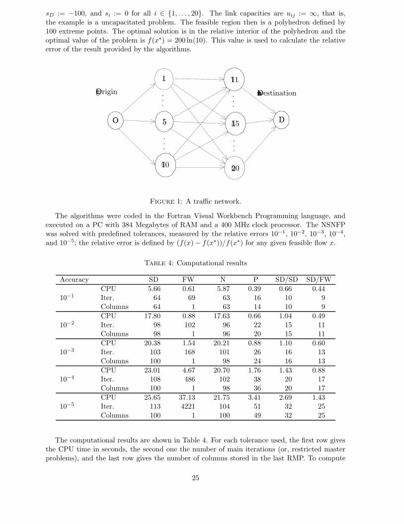
sD := −100, and si := 0 for all i ∈ 1, . . . , 20. The link capacities are uij := ∞, that is,the example is a uncapacitated problem. The feasible region then is a polyhedron defined by100 extreme points. The optimal solution is in the relative interior of the polyhedron and theoptimal value of the problem is f(x∗) = 200 ln(10). This value is used to calculate the relativeerror of the result provided by the algorithms.

Origin Destination

1

O 5

10

11

15

20

D

.

.

.

.

.

.

.

.

.

.

.

.

Figure 1: A traffic network.

The algorithms were coded in the Fortran Visual Workbench Programming language, andexecuted on a PC with 384 Megabytes of RAM and a 400 MHz clock processor. The NSNFPwas solved with predefined tolerances, measured by the relative errors 10−1, 10−2, 10−3, 10−4,and 10−5; the relative error is defined by (f(x) − f(x∗))/f(x∗) for any given feasible flow x.

Table 4: Computational results

Accuracy SD FW N P SD/SD SD/FW

10−1CPUIter.Columns

5.666464

0.61691

5.876363

0.391614

0.661010

0.4499

10−2CPUIter.Columns

17.809898

0.88102

1

17.639696

0.662220

1.041515

0.491111

10−3CPUIter.Columns

20.38103100

1.54168

1

20.2110198

0.882624

1.101616

0.601313

10−4CPUIter.Columns

23.01108100

4.67486

1

20.7010298

1.763836

1.432020

0.881717

10−5CPUIter.Columns

25.65113100

37.134221

1

21.75104100

3.415149

2.693232

1.432525

The computational results are shown in Table 4. For each tolerance used, the first row givesthe CPU time in seconds, the second one the number of main iterations (or, restricted masterproblems), and the last row gives the number of columns stored in the last RMP. To compute

25

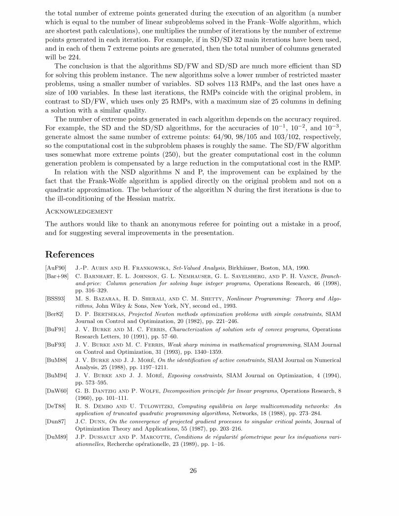
the total number of extreme points generated during the execution of an algorithm (a numberwhich is equal to the number of linear subproblems solved in the Frank–Wolfe algorithm, whichare shortest path calculations), one multiplies the number of iterations by the number of extremepoints generated in each iteration. For example, if in SD/SD 32 main iterations have been used,and in each of them 7 extreme points are generated, then the total number of columns generatedwill be 224.

The conclusion is that the algorithms SD/FW and SD/SD are much more efficient than SDfor solving this problem instance. The new algorithms solve a lower number of restricted masterproblems, using a smaller number of variables. SD solves 113 RMPs, and the last ones have asize of 100 variables. In these last iterations, the RMPs coincide with the original problem, incontrast to SD/FW, which uses only 25 RMPs, with a maximum size of 25 columns in defininga solution with a similar quality.

The number of extreme points generated in each algorithm depends on the accuracy required.For example, the SD and the SD/SD algorithms, for the accuracies of 10−1, 10−2, and 10−3,generate almost the same number of extreme points: 64/90, 98/105 and 103/102, respectively,so the computational cost in the subproblem phases is roughly the same. The SD/FW algorithmuses somewhat more extreme points (250), but the greater computational cost in the columngeneration problem is compensated by a large reduction in the computational cost in the RMP.

In relation with the NSD algorithms N and P, the improvement can be explained by thefact that the Frank-Wolfe algorithm is applied directly on the original problem and not on aquadratic approximation. The behaviour of the algorithm N during the first iterations is due tothe ill-conditioning of the Hessian matrix.

Acknowledgement

The authors would like to thank an anonymous referee for pointing out a mistake in a proof,and for suggesting several improvements in the presentation.

References

[AuF90] J.-P. Aubin and H. Frankowska, Set-Valued Analysis, Birkhauser, Boston, MA, 1990.

[Bar+98] C. Barnhart, E. L. Johnson, G. L. Nemhauser, G. L. Savelsberg, and P. H. Vance, Branch-and-price: Column generation for solving huge integer programs, Operations Research, 46 (1998),pp. 316–329.

[BSS93] M. S. Bazaraa, H. D. Sherali, and C. M. Shetty, Nonlinear Programming: Theory and Algo-rithms, John Wiley & Sons, New York, NY, second ed., 1993.

[Ber82] D. P. Bertsekas, Projected Newton methods optimization problems with simple constraints, SIAMJournal on Control and Optimization, 20 (1982), pp. 221–246.

[BuF91] J. V. Burke and M. C. Ferris, Characterization of solution sets of convex programs, OperationsResearch Letters, 10 (1991), pp. 57–60.

[BuF93] J. V. Burke and M. C. Ferris, Weak sharp minima in mathematical programming, SIAM Journalon Control and Optimization, 31 (1993), pp. 1340–1359.

[BuM88] J. V. Burke and J. J. More, On the identification of active constraints, SIAM Journal on NumericalAnalysis, 25 (1988), pp. 1197–1211.

[BuM94] J. V. Burke and J. J. More, Exposing constraints, SIAM Journal on Optimization, 4 (1994),pp. 573–595.

[DaW60] G. B. Dantzig and P. Wolfe, Decomposition principle for linear programs, Operations Research, 8(1960), pp. 101–111.

[DeT88] R. S. Dembo and U. Tulowitzki, Computing equilibria on large multicommodity networks: Anapplication of truncated quadratic programming algorithms, Networks, 18 (1988), pp. 273–284.

[Dun87] J.C. Dunn, On the convergence of projected gradient processes to singular critical points, Journal ofOptimization Theory and Applications, 55 (1987), pp. 203–216.

[DuM89] J.P. Dussault and P. Marcotte, Conditions de regularite geometrique pour les inequations vari-ationnelles, Recherche operationelle, 23 (1989), pp. 1–16.

26

[Eva76] S. P. Evans, Derivation and analysis of some models for combining trip distribution and assignment,Transportation Research, 10 (1976), pp. 37–57.

[Fuk92] M. Fukushima, Equivalent differentiable optimization problems and descent methods for asymmetricvariational inequality problems, Mathematical Programming, 53 (1992), pp. 99–110.

[GaM97a] R. Garcıa and A. Marın, Urban multimodal interchanges (Macro Vision), conference presentation atthe EURO XV–INFORMS XXXIV Joint International Meeting, Barcelona, July 14–17, 1997.

[GaM97b] R. Garcıa and A. Marın, Using RSD within partial linearization methods, conference presentation atthe 16th International Symposium on Mathematical Programming, Lausanne, August 24–29, 1997.

[GMP02] R. Garcıa, A. Marın, and M. Patriksson, Column generation algorithms for nonlinear optimization,II: Numerical investigations, report, Department of Mathematics, Chalmers University of Technology,Gothenburg, Sweden, 2001 (to appear).

[GHV92] J.-L. Goffin, A. Haurie, and J.-P. Vial, Decomposition and nondifferentiable optimization withthe projective algorithm. Management Science, 37 (1992), pp. 284–302.

[Gol64] A. A. Goldstein, Convex programming in Hilbert space, Bulletin of the American MathematicalSociety, 70 (1964), pp. 709–710.

[Gui69] M. Guignard, Generalized Kuhn–Tucker conditions for mathematical programming problems in aBanach space, SIAM Journal on Control, 7 (1969), pp. 232–241.

[Ham84] J. H. Hammond, Solving asymmetric variational inequality problems and systems of equationswith generalized nonlinear programming algorithms, PhD thesis, Department of Mathematics, Mas-sachusetts Institute of Technology, Cambridge, MA, 1984.

[HaP90] P. T. Harker and J.-S. Pang, Finite-dimensional variational inequality and nonlinear complemen-tarity problems: A survey of theory, algorithms and applications, Mathematical Programming, 48(1990), pp. 161–220.

[HLV85] D. W. Hearn, S. Lawphongpanich, and J. A. Ventura, Finiteness in restricted simplicial decom-position, Operations Research Letters, 4 (1985), pp. 125–130.

[HLV87] D. W. Hearn, S. Lawphongpanich, and J. A. Ventura, Restricted simplicial decomposition:Computation and extensions, Mathematical Programming Study, 31 (1987), pp. 99–118.

[HiP90] J. E. Higgins and E. Polak, Minimizing pseudoconvex functions on convex compact sets, Journalof Optimization Theory and Applications, 65 (1990), pp. 1–27.

[Hol74] C. A. Holloway, An extension of the Frank and Wolfe method of feasible directions, MathematicalProgramming, 6 (1974), pp. 14–27.

[HoJ61] R. Hooke and T. A. Jeeves, Direct search solution of numerical and statistical problems, Journalof the Association for Computer Machinery, 8 (1961), pp. 212–229.

[JTPR94] R. Jayakrishnan, W. K. Tsai, J. N. Prashker, and S. Rajadhyaksha, Faster path-based algo-rithm for traffic assignment, Transportation Research Record, 1443 (1994), pp. 75–83.

[JLF93] K. L. Jones, I. J. Lustig, J. M. Farvolden, and W. B. Powell, Multicommodity network flows:The impact of formulation on decomposition, Mathematical Programming, 62 (1993), pp. 95–117.

[KiN91] K. Kim and J. L. Nazareth, The decomposition principle and algorithms for linear programming,Linear Algebra and Its Applications, 152 (1991), pp. 119–133.

[LMP94] T. Larsson, A. Migdalas, and M. Patriksson, A generic column generation scheme, Report LiTH-MAT-R-94-18, Department of Mathematics, Linkoping Institute of Technology, Linkoping, Sweden,1994. Revised version, July 1999.

[LaP92] T. Larsson and M. Patriksson, Simplicial decomposition with disaggregated representation for thetraffic assignment problem, Transportation Science, 26 (1992), pp. 4–17.

[LPR97] T. Larsson, M. Patriksson, and C. Rydergren, Applications of simplicial decomposition withnonlinear column generation to nonlinear network flows, in Network Optimization, P. M. Pardalos,W. W. Hager, and D. W. Hearn, eds., Springer-Verlag, Berlin, 1997, pp. 346–373.

[Las70] L. S. Lasdon, Optimization Theory for Large Systems, Macmillan, New York, NY, 1970.

[LaH84] S. Lawphongpanich and D. W. Hearn, Simplicial decomposition of the asymmetric traffic assign-ment problem, Transportation Research, 18B (1984), pp. 123–133.

[LeP66] E. S. Levitin and B. T. Polyak, Constrained minimization methods, USSR Computational Math-ematics and Mathematical Physics, 6 (1966), pp. 1–50.

[Lue84] D. G. Luenberger, Linear and Nonlinear Programming, Addison-Wesley, Reading, MA, second ed.,1984.

[LuP98] J. T. Lundgren and M. Patriksson, An algorithm for the combined distribution and assignmentmodel, in Transportation Networks: Recent Methodological Advances, Selected Proceedings of the 4thEURO Transportation Meeting, Newcastle University, Newcastle, UK, September 9–11, 1996, M. G.H. Bell (ed.), Pergamon Press, Amsterdam, 1998, pp. 239–253.

27

[MaD89] P. Marcotte and J.-P. Dussault, A sequential linear programming algorithm for solving monotonevariational inequalities, SIAM Journal on Control and Optimization, 27 (1989), pp. 1260–1278.

[MaZ98] P. Marcotte and D. Zhu, Weak sharp solutions of variational inequalities, SIAM Journal on Opti-mization, 9 (1998), pp. 179–189.

[Mig94] A. Migdalas, A regularization of the Frank–Wolfe method and unification of certain nonlinear pro-gramming methods, Mathematical Programming, 65 (1994), pp. 331–345.

[Pat93a] M. Patriksson, Partial linearization methods in nonlinear programming, Journal of OptimizationTheory and Applications, 78 (1993), pp. 227–246.

[Pat93b] M. Patriksson, A unified description of iterative algorithms for traffic equilibria, European Journalof Operational Research, 71 (1993), pp. 154–176.

[Pat98a] M. Patriksson, Cost approximation: A unified framework of descent algorithms for nonlinear pro-grams, SIAM Journal on Optimization, 8 (1998), pp. 561–582.

[Pat98b] M. Patriksson, Nonlinear Programming and Variational Inequality Problems—A Unified Approach,Kluwer Academic Publishers, Utrecht, The Netherlands, 1998.

[Pol87] B. T. Polyak, Introduction to Optimization, Optimization Software, New York, NY, 1987.

[Roc70] R. T. Rockafellar, Convex Analysis, Princeton University Press, Princeton, NJ, 1970.

[RoW98] R. T. Rockafellar and R. J.-B. Wets, Variational Analysis, Springer-Verlag, Berlin, 1998.

[Rud76] W. Rudin, Principles of Mathematical Analysis, Third Edition, McGraw-Hill, Auckland, 1976.

[SaW79] G. Salinetti and R.-B. Wets, On the convergence of sequences of convex sets in finite dimensions,SIAM Review, 21 (1979), pp. 18–33.

[Tse91] P. Tseng, Decomposition algorithm for convex differentiable minimization, Journal of OptimizationTheory and Applications, 70 (1991), pp. 109–135.

[VeH93] J. A. Ventura and D. W. Hearn, Restricted simplicial decomposition for convex constrained prob-lems, Mathematical Programming, 59 (1993), pp. 71–85.

[vHo77] B. Von Hohenbalken, Simplicial decomposition in nonlinear programming algorithms, MathematicalProgramming, 13 (1977), pp. 49–68.

[Wol70] P. Wolfe, Convergence theory in nonlinear programming, in Integer and Nonlinear Programming, J.Abadie (ed.), North-Holland, New York, NY, 1970, pp. 1–36.

[Wol98] L. A. Wolsey. Integer Programming. John Wiley & Sons, New York, NY, 1998.

[Zan69] W. I. Zangwill, Nonlinear Programming: A Unified Approach, Prentice-Hall, Englewood Cliffs, NJ,1969.

[ZhM95] D. L. Zhu and P. Marcotte, Coupling the auxiliary problem principle with descent methods ofpseudoconvex programming, European Journal of Operational Research, 83 (1995), pp. 670–685.

28