COLUMN ABUNDANCES OF CARBON DIOXIDE AND ...api/deki/files/309/...keeping my Ph.D. on track and aimed...

COLUMN ABUNDANCES OF CARBON DIOXIDE AND METHANE RETRIEVED

FROM GROUND-BASED NEAR-INFRARED SOLAR SPECTRA

Thesis by

Rebecca A. Washenfelder

In Partial Fulfillment of the Requirements for the Degree of

Doctor of Philosophy

CALIFORNIA INSTITUTE OF TECHNOLOGY

Pasadena, California

2006

(Defended May 22, 2006)

ii

© 2006

Rebecca A. Washenfelder

All Rights Reserved

iii

Acknowledgements

Most importantly, I thank my advisor, Paul Wennberg, who welcomed me to Caltech. I

truly appreciate his guidance, and I am continually inspired by his clear insight into

scientific problems. As a member of Paul’s group, I have enjoyed the opportunity to work

on exciting research projects and travel throughout the world. In addition to Paul, I thank

my committee members, Mitchio Okumura, James Randerson, and Geoffrey Toon for

keeping my Ph.D. on track and aimed toward completion.

I thank Geoffrey Toon and Jean-Francois Blavier for the enormous amount of time and

energy they have invested in teaching me about Linux, Fourier Transform spectrometry,

and a dozen other topics. Zhonghua Yang and Gretchen Aleks have been great friends and

collaborators in this project. I thank Gretchen for adopting the Park Falls observatory and

continuing this project into the future. I enjoyed assembling the second observatory and

traveling to Australia with Yael Yavin. Yael’s independence in assembling the third

observatory with Gretchen has been invaluable in making my thesis writing possible. I

appreciate the instruction I received from Dave Petterson in electronics and cable-making.

I thank Norton Allen for his work in automating the Fourier Transform spectrometer data

acquisition. The volley of emails between Jean-Francois Blavier and Norton Allen has

been educational, even if I couldn’t always keep up.

Caltech has been an accommodating place for instrumental work. I thank Mark Harriman

and the Athletic Center staff for providing space for the observatories. It was pleasant to

spend so many hours near the swimming pool. Among the many people on campus who

helped with this project, I would particularly like to thank Rick Gerhart from the

Glassblowing Shop, Rick Germond from the Central Warehouse, Corey Campbell and

Moses from the Main Stockroom, and Mike Anchondo from the Electrical Shop. I thank

the Physics Machine Shop staff, especially Armando De Las Casas and Rick Paniagua who

guided me during the many happy hours I spent there. Leticia Calderon and Irma Black

have smoothed the way administratively whenever there has been trouble. Thanks to

iv

Michael Black, David Kewley, and Scott Dungan for setting up the RAID and solving my

computer troubles.

Beyond Caltech, I have enjoyed my ongoing collaboration with Nick Deutscher, David

Griffith, and Glenn Bryant at the University of Wollongong, and with Brian Connor and

Vanessa Sherlock at NIWA. Thanks to Ankur Desai, Dan Ricciuto, and Ken Davis at

Pennsylvania State University for sharing their data and answering my many questions

about eddy covariance measurements. Thanks to Linda Brown for her insight into

laboratory spectroscopy. Finally, I would like to thank Ross Salawitch, Charles Miller,

David Crisp, and the OCO science team.

I have thoroughly enjoyed my time in the Wennberg group with Karena McKinney, Suresh

Dhaniyala, Coleen Roehl, Zhonghua Yang, Julie Fry, John Crounse, Alan Kwan, Yael

Yavin, Gretchen Aleks, and David McCabe. I will miss our lunch routine at the South

Lake Italian Kitchen. My first year of coursework at Caltech was vastly improved by

friendships with Lisa Welp, Megan Ferguson, Jamie Lindfors, and Jeff Mendez. I have

enjoyed many subsequent adventures hiking, canyoneering, and cycling with Lisa and

Megan.

At Pomona College, I was lucky to have professors who believed in me and gave me useful

career advice, especially Professor Daniel O’Leary. Finally, I thank my family for their

love and support.

v

Abstract

To predict future climate change, we must accurately predict future atmospheric

concentrations of CO2 and CH4. The current budget has typically been inferred from top-

down analyses of measurements from a global network of surface sites. These

measurements are highly accurate, but have limited spatial coverage. In addition, accurate

knowledge of local planetary boundary layer dynamics is necessary to determine fluxes.

Column measurements, defined as the vertical integral of gas concentration, can

complement the existing in situ network. Because column measurements sample a larger

portion of the atmosphere, they exhibit less variability than surface data, while retaining

information about surface fluxes. Column measurements are not influenced by planetary

boundary layer dynamics, and do not suffer from the resulting correlation between

exchange and transport.

An automated observatory for measuring ground-based column abundances of CO2, CH4,

and O2 is described. Near-infrared spectra of the direct sun are obtained from 3,900 –

15,600 cm-1 by a Bruker 125HR Fourier transform spectrometer. The observatory was

assembled in Pasadena, California and then permanently deployed to Northern Wisconsin

during May 2004. Under clear sky conditions, retrieved column CO2 abundances

demonstrate ~0.1% precision. Comparison of these column measurements with eight

aircraft profiles of in situ CO2 recorded during summer 2004 shows a small bias, but an

excellent correlation.

The observed secular increase and seasonal amplitude of column-average CO2 observed

during the period of May 2004 – March 2006 is 1.8 ppmv yr-1 and 11 ppmv, consistent

with theoretical predictions that the measurements will be representative of Northern

Hemisphere CO2 exchange over seasonal timescales. Comparisons with eddy covariance

measurements show that the column measurements have potential for directly observing

CO2 exchange, but that this ability is constrained by the difficulty in accounting for

atmospheric transport.

vi

Finally, the use of near-infrared spectral analysis is extended to observations of

tropospheric column-average CH4 concentrations. By employing a stratospheric “slope

equilibrium” relationship between CH4 and HF, the varying contribution of stratospheric

CH4 to the total column is inferred. This method is used to determine tropospheric column-

average CH4 VMRs from near-infrared solar absorption spectra recorded at the Kitt Peak

National Solar Observatory during 1977 – 1995.

vii

Contents

Acknowledgements ................................................................................................................ iii

Abstract .....................................................................................................................................v

Contents ..................................................................................................................................vii

List of Figures .........................................................................................................................xii

List of Tables ........................................................................................................................ xiii

List of Abbreviations .............................................................................................................xiv

Chapter 1 Introduction.......................................................................................................... 1-1

1.1 The Global Carbon Budget ........................................................................................ 1-1

1.2 Remote Sensing Techniques ...................................................................................... 1-3

1.3 Outline of the Dissertation ......................................................................................... 1-5

1.4 References................................................................................................................... 1-6

Chapter 2 Carbon Dioxide Column Abundances at the Wisconsin Tall Tower Site ......... 2-1

2.1 Abstract....................................................................................................................... 2-1

2.2 Introduction................................................................................................................. 2-1

2.3 Instrumentation........................................................................................................... 2-3

2.3.1 Bruker 125HR Spectometer................................................................................ 2-3

2.3.2 Laboratory and Other Instrumentation ............................................................... 2-5

2.3.3 Data Acquisition and Instrumental Automation................................................. 2-8

2.4 Measurement Site ....................................................................................................... 2-9

2.5 Data Analysis............................................................................................................ 2-10

2.5.1 Column O2 and CO2.......................................................................................... 2-12

2.6 Comparison of FTS Column and Integrated Aircraft Profiles................................ 2-17

2.6.1 Error Analysis for Column-Average CO2 VMR.............................................. 2-22

2.6.2 Column-Average CO2 VMR During May 2004 – October 2005.................... 2-24

2.6.3 Conclusions ....................................................................................................... 2-25

2.7 Acknowledgements .................................................................................................. 2-26

viii

2.8 References................................................................................................................. 2-26

Chapter 3 Surface Exchange of CO2 Observed by Coincident Eddy Covariance Flux and

Column Measurements......................................................................................................... 3-1

3.1 Abstract....................................................................................................................... 3-1

3.2 Introduction................................................................................................................. 3-1

3.3 Column Measurements: Instrumentation and Data Analysis.................................... 3-4

3.4 Research Site .............................................................................................................. 3-4

3.5 Seasonal CO2 Exchange............................................................................................. 3-6

3.5.1 Park Falls WLEF Site During 2004 – 2005 ....................................................... 3-6

3.5.2 Comparison to TransCom Model Predictions.................................................... 3-7

3.6 Local CO2 Exchange .................................................................................................. 3-9

3.6.1 Bottom-Up Estimates of Local CO2 Exchange. ................................................. 3-9

3.6.2 Eddy Covariance: Instrumentation and Data Analysis .................................... 3-11

3.6.3 Calculation of Net Ecosystem Exchange from the Total Column................... 3-11

3.6.4 Comparison of Drawdown Observed by FTS and Eddy Covariance.............. 3-15

3.7 Conclusions............................................................................................................... 3-18

3.8 References................................................................................................................. 3-19

Chapter 4 Tropospheric Methane Retrieved From Ground-Based Near-Infrared Solar

Absorption Spectra ............................................................................................................... 4-1

4.1 Abstract....................................................................................................................... 4-1

4.2 Introduction................................................................................................................. 4-1

4.3 Determination of Tropospheric CH4.......................................................................... 4-2

4.4 The Kitt Peak Spectra................................................................................................. 4-4

4.5 Spectral Analysis and Retrievals................................................................................ 4-5

4.6 Tropospheric CH4 Volume Mixing Ratios ................................................................ 4-8

4.7 Conclusions............................................................................................................... 4-11

4.8 Acknowledgments .................................................................................................... 4-12

4.9 Appendix: Pressure Broadening of the CH4 2ν3 Band ............................................ 4-12

4.10 Appendix: Correlation of HF and CH4 in the Lower and Mid Stratosphere: the

Determination of b(t) ...................................................................................................... 4-13

ix

4.11 References............................................................................................................... 4-16

Appendix Technical Documentation for the Caltech Column Observatory....................... 5-1

A.1 Summary.................................................................................................................... 5-1

A.2 Instrumentation.......................................................................................................... 5-2

A.2.1 Bruker IFS125 Spectrometer ............................................................................. 5-2

A.2.1.1 Laser (Spectra-Physics 117A) .................................................................... 5-2

A.2.1.2 Scanner ........................................................................................................ 5-3

A.2.1.3 Detectors...................................................................................................... 5-3

A.2.1.4 Tungsten Lamp............................................................................................ 5-4

A.2.1.5 Valves and Vacuum System ....................................................................... 5-5

A.2.1.6 Small Devices with Control Area Network Boards ................................... 5-6

A.2.1.7 Electronics Systems .................................................................................... 5-6

A.2.1.8 HTML Software Interface .......................................................................... 5-8

A.2.1.9 IFS125 Direct Commands and Allowed Values ........................................ 5-9

A.2.1.10 Alignment Procedure .............................................................................. 5-12

A.2.1.11 Previous Alignment Results ................................................................... 5-16

A.2.1.12 Acceptance Test Standards ..................................................................... 5-17

A.2.1.13 HCl Cells ................................................................................................. 5-19

A.2.2 Bruker Solar Tracker........................................................................................ 5-20

A.2.2.1 Solar Tracker Direct RS232 Commands.................................................. 5-20

A.2.2.2 Solar Tracker Installation.......................................................................... 5-21

A.2.3 Telescope Dome............................................................................................... 5-23

A.2.3.1 Dome Direct RS232 Commands: ............................................................. 5-24

A.2.4 Weather Station ................................................................................................ 5-25

A.2.4.1 Direct RS232 Commands: ........................................................................ 5-25

A.2.4.2 Barometric Pressure (S1080Z) ................................................................. 5-25

A.2.4.3 Relative Humidity and Air Temperature (S1276Z) ................................. 5-26

A.2.4.4 Wind Speed and Direction (S1146Z) ....................................................... 5-26

A.2.4.5 Pyranometer (S1114Z).............................................................................. 5-26

A.2.4.6 Precipitation Detector (S1391Z)............................................................... 5-26

A.2.4.7 Leaf Wetness Sensor (S1169)................................................................... 5-26

x

A.2.4.8 Mercury Manometer ................................................................................. 5-26

A.2.5 Other Laboratory Instrumentation ................................................................... 5-28

A.2.5.1 NTP-GPS Receiver ................................................................................... 5-28

A.2.5.2 Network Camera ....................................................................................... 5-28

A.2.5.3 Scroll Pump............................................................................................... 5-28

A.2.5.4 Scroll Pump Pressure Sensor .................................................................... 5-29

A.2.6 Network and Communication.......................................................................... 5-30

A.2.6.1 Network Information ................................................................................ 5-30

A.2.6.2 Modem....................................................................................................... 5-30

A.2.7 Power Systems ................................................................................................. 5-31

A.2.7.1 Uninterruptible Power Supply .................................................................. 5-31

A.2.8 Digital and Analog Signals .............................................................................. 5-32

A.2.8.1 Control Using Digital Lines...................................................................... 5-32

A.2.8.2 Monitoring of Analog Inputs .................................................................... 5-32

A.2.8.3 Reference and Background Information .................................................. 5-33

A.2.9 Laboratory structure ......................................................................................... 5-35

A.2.9.1 Container ................................................................................................... 5-35

A.2.9.2 Heater – Air Conditioner Unit .................................................................. 5-35

A.3 Data Acquisition Software ...................................................................................... 5-36

A.3.1 Data Acquisition Software Overview.............................................................. 5-36

A.3.2 Data Acquisition Source Code Files................................................................ 5-37

A.3.3 Organization of Data ........................................................................................ 5-40

A.3.4 Telemetry Data ................................................................................................. 5-42

A.3.5 Quick Command Tree for ifsdoit..................................................................... 5-45

A.3.6 Detailed Description of ifsdoit Commands .................................................... 5-47

A.3.7 Routine Monitoring of the Data Acquisition................................................... 5-51

A.3.8 Queuing Directories to Repeat the Overnight Analysis.................................. 5-52

A.3.9 Hercules Computer Shutdown Instructions..................................................... 5-52

A.3.10 Useful QNX Commands ................................................................................ 5-53

A.3.11 CVS Software Archive................................................................................... 5-54

A.4 Data Transfer, Archive, and Processing ................................................................. 5-56

xi

A.4.1 Removable Disks.............................................................................................. 5-56

A.4.2 RAID at Caltech ............................................................................................... 5-58

A.4.3 MD5SUM Tool: dircksum............................................................................... 5-60

A.4.4 Slice-IPP Fourier Transform Software ............................................................ 5-61

A.4.4.1 Fourier-Transform Using Slice-IPP.......................................................... 5-61

A.4.4.2 Bruker Acronyms Contained in the IFS125 Spectral Headers ................ 5-61

A.4.4.3 Additional Acronyms Defined for the IFS125 Spectral Headers ........... 5-63

A.4.4.4 Filenaming Convention............................................................................. 5-64

A.5 General Logistics..................................................................................................... 5-65

A.5.1 Contact Information and Account Numbers.................................................... 5-65

A.5.2 Caltech FTS Site............................................................................................... 5-66

A.5.2.1 Caltech Contact Information and Logistics.............................................. 5-66

A.5.2.2 Caltech Network Connectivity ................................................................. 5-66

A.5.3 Park Falls FTS Site........................................................................................... 5-67

A.5.3.1 Park Falls Contact Information and Logistics.......................................... 5-67

A.5.3.2 Park Falls Network Connectivity ............................................................. 5-68

A.5.4 Darwin FTS Site............................................................................................... 5-70

A.5.4.1 Darwin Contact Information and Logistics .............................................. 5-70

A.5.4.2 Darwin Network Connectivity.................................................................. 5-71

xii

List of Figures

Figure 2.1 Photograph and Block Diagram of the Automated FTS Observatory. ..............2-4

Figure 2.2 Signal-to-Noise Ratio and Near-IR Absorptions in FTS Solar Spectrum..........2-6

Figure 2.3 Correlation Between Retrieved Column O2 and Dry Surface Pressure. ..........2-14

Figure 2.4 Spectral Retrievals During One Clear and One Partly Cloudy Day.................2-16

Figure 2.5 Aircraft Profile Measurement of In Situ CO2.. .................................................2-21

Figure 2.6 Comparison of Column and Integrated Aircraft CO2 Profiles .........................2-22

Figure 2.7 Diurnal and Seasonal Column CO2 Measurements. .........................................2-25

Figure 3.1 WISCLAND Landcover Classification...............................................................3-5

Figure 3.2 Column, In Situ, and Eddy Covariance Measurements of CO2.. .......................3-7

Figure 3.3 TransCom Model Predictions of Seasonal Cycle.. .............................................3-9

Figure 3.4 Demonstration of Column and Eddy Covariance Observations of NEE. ........3-15

Figure 3.5 Column CO2 Change Attributed to NEE and Transport...................................3-16

Figure 3.6 Drawdown Observed During a Four-Hour Period...........................................3-18

Figure 4.1 Spectral Fits of CH4 and HF for a Kitt Peak Solar Absorption Spectrum. ........4-7

Figure 4.2 Time Series of Column-Average CH4 and Column HF. ....................................4-8

Figure 4.3 CH4–HF Slope Values from the HALOE, MkIV, and Kitt Peak Data. .............4-9

Figure 4.4 Time Series of Kitt Peak Tropospheric CH4 VMR...........................................4-10

Figure 4.5 Determination of CH4–HF Slope Values. .........................................................4-14

Figure 4.6 CH4 and HF Averaging Kernels for a Kitt Peak Spectrum . ............................4-15

xiii

List of Tables

Table 2.1. Mean and standard deviation of column CO2 measurements during a

one-hour observational period around local noon..................................................2-16

xiv

List of Abbreviations

CASA– Carnegie-Ames-Stanford Approach biogeochemical model

COBRA – CO2 Boundary-layer Regional Airborne experiment

FTS – Fourier transform spectrometry or Fourier transform spectrometer

GAGE/AGAGE – Global Atmospheric Gases Experiment / Advanced Global Atmospheric

Gases Experiment

GFIT – Spectral retrieval analysis software

GOSAT – Greenhouse Gases Observing Satellite

HALOE – Halogen Occultation Experiment

HITRAN – High-Resolution Transmission molecular absorption database

INTEX-NA – Intercontinental Chemical Transport Experiment – North America

MATCH – Multiscale Atmospheric Transport and Chemistry model

MOPPIT – Measurements of Pollution in the Troposphere

NDSC – Network for the Detection of Stratospheric Change

NEE – Net Ecosystem Exchange

OCO – Orbiting Carbon Observatory

SCIAMACHY – Scanning Imaging Absorption Spectrometer for Atmospheric

Chartography

SZA – Solar Zenith Angle

xv

TCCON – Total Carbon Column Observing Network

TransCom – Atmospheric Tracer Transport Model Intercomparison Project

UARS – Upper Atmosphere Research Satellite

WISCLAND – Wisconsin Initiative for Statewide Cooperation on Landscape Analysis and

Data

1-1

Chapter 1

INTRODUCTION

1.1 The Global Carbon Budget

An increasing body of observations gives a collective picture of a warming world and other

changes in the climate system [(IPCC), 2001]. The atmospheric constituents with current

importance to climate are H2O, CO2, O3, CH4, N2O, CFC-11, and CFC-12 [Ramanathan et

al., 1987]. Close correlations between CO2, CH4, and temperature are observed in the

Vostok ice core record during the past 420,000 years [Petit et al., 1999; Fischer et al.,

1999], suggesting that past climate change is in part forced by changes in atmospheric

concentrations of greenhouse gases. Although the atmospheric concentration of CH4 and

the magnitude of CH4 fluxes are much lower than that of CO2 [Fung et al., 1991;

Houweling et al., 1999], CH4 plays an important role in the Earth’s radiative balance. The

instantaneous forcing of each additional CH4 molecule in the atmosphere is 43 times

greater than that for a molecule of CO2 [Lashof and Ahuja, 1990]. Better understanding of

both CO2 and CH4 is critical to predicting the Earth’s radiative budget.

The global budgets of CO2 and CH4 have been altered by anthropogenic activity.

Atmospheric CO2 concentrations have increased from 280 ppmv in pre-industrial times to

~370 ppmv in 1999, and are currently increasing at a rate of 1 – 2 pppmv yr-1 [(IPCC),

2001]. This increase is mainly anthropogenic, and is attributed to fossil fuel consumption

[Marland, 2000] and land use change [Houghton, 1999]. The net global release of CO2

caused by the burning of fossil fuels is one of the best-known values in the global carbon

cycle [Marland, 2000]. The discrepancy between CO2 release by burning of fossil fuels

and CO2 accumulation in the atmosphere is attributed to uptake by oceans and the

terrestrial biosphere [Battle et al., 2000; Keeling et al., 1993; Keeling and Shertz, 1992].

CH4 concentrations have also increased rapidly, from ~0.685 ppmv to ~1.745 ppmv

between 1750 and 1998 [Dlugokencky et al., 1998]. During the past two decades, the

growth rate of CH4 has varied between 0 and 0.015 ppmv yr-1 [Dlugokencky et al., 1998],

1-2

but the cause of this variability is poorly understood. The decline in growth rate may be

due to decreased northern wetland emission rates [Hogan and Harriss, 1994] or increases

in tropospheric OH [Bekki et al., 1994]. Isotopic records of atmospheric CH4 suggest an

anomaly in sources or sinks involving more than one causal factor [Lowe et al., 1997; Mak

et al., 2000]. The variable increase of atmospheric CH4 is likely due to a small imbalance

between poorly-characterized sources and sinks.

It is clear that a significant source of uncertainty in the prediction of climate change is the

future concentrations of the greenhouse gases themselves [Rayner et al., 1996].

Uncertainty in future trends for these gases arises from uncertainty in their current budget.

After 30 years of measurements in the atmosphere and oceans, many unknowns still remain

in the global CO2 budget. The magnitude of sources and sinks of CO2 and other

greenhouse gases are currently inferred from in situ measurements at two global networks

of surface sites, operated by the National Oceanic and Atmospheric Administration

(NOAA) and the Scripps Institute of Oceanography [GLOBALVIEW-CO2, 2005; Conway

et al., 1994; Keeling et al., 1995]. Studies have combined in situ measurements of CO2

with global scale transport models to estimate regional-scale surface exchange of CO2

using inversion techniques [Gurney et al., 2002; Rayner et al., 1999; Tans et al., 1990].

This has proven difficult, in part due to limitations in the surface measurements. Although

the measurements are highly accurate, they have limited spatial coverage, are confined to

the planetary boundary layer, and are biased to specific weather conditions. Because

exchange and transport are correlated on diurnal and seasonal timescales, errors in transport

fields may be aliased into the inferred exchange terms as “rectifier” effects [Denning et al.,

1996a; Gurney et al., 2002].

The atmospheric column integral of CO2 and CH4 may be effective in constraining the

global carbon budget [Olsen and Randerson, 2004]. Column measurements sample a

larger portion of the atmosphere than surface in situ measurements. Because the column is

insensitive to vertical mixing, the column integral should be largely unaffected by diurnal

fluctuations in the boundary layer and should exhibit much less variability than surface

data, thus avoiding rectifier effects while retaining information about surface fluxes [Gloor

et al., 2000]. Model predictions show that a few column measurements at carefully

1-3

selected sites could constrain the global carbon budget [Gloor et al., 2000; Rayner and

O'Brien, 2001].

1.2 Remote Sensing Techniques

Remote sensing methods can be used to obtain the column integrals of CO2, CH4, and other

atmospheric species. Because molecules possess quantized internal energy levels, they

absorb and emit electromagnetic radiation at discrete frequencies. The electromagnetic

spectrum of the atmosphere contains features that are characteristic of its constituents, and

can be used for their identification and quantification. The features that we observe in the

atmosphere are due to electronic, vibrational, and rotational transitions of molecules and

atoms. Electronic transitions are typically observed in the visible and ultraviolet spectral

regions. Vibrational transitions are observed in the near-infrared and mid-infrared spectral

regions. Rotational transitions within a vibrational state are observed in the far-infrared

and microwave spectral regions. Atmospheric remote sensing is possible from the ground,

from aircraft, from balloons, and from space, with observation of radiation either from an

external source (absorption spectroscopy) or from the atmospheric blackbody signal

(emission spectroscopy).

Solar absorption spectroscopy has been used to measure the Earth’s atmosphere for over a

century. The solar absorption spectrum was first measured by Joseph von Fraunhofer using

a grating instrument. In 1879, Marie Alfred Cornu predicted that the short wavelength

limit of the observed solar radiation must be caused by an absorber in the Earth’s

atmosphere [Cornu, 1879b; Cornu, 1879a; Cornu, 1890]. This correct deduction of the

strong UV O3 absorptions was followed by identifications from Sir Walther Noel Hartley,

J. Chappuis, and Sir William Huggins [Hartley, 1881; Huggins, 1889]. By the 20th century,

ground-based remote infrared sensing used prisms and grating spectrometers to measure

the sun’s light. High-altitude observatories minimized spectral interference, and

measurements at sunset and sunrise maximized the atmospheric path for improved

detection of trace species. The first systematic study of solar irradiance at the Earth’s

surface was conducted by Samuel Pierpont Langely, using these methods at the summit of

Mt. Whitney, California [Langley, 1900]. A stable spectrometer, using a double

monochromator with quartz prisms, was developed by Gordon M. B. Dobson to quantify

1-4

the vertical column density of O3 [Dobson, 1968]. The Dobson spectrometer is the direct

predecessor of modern-day atmospheric remote sensing.

Fourier Transform Spectrometry (FTS) is the direct descendant of these early spectroscopic

measurements. The FTS is an adapted Michelson interferometer [Michelson, 1891;

Michelson, 1892] with a movable mirror. After a collimated beam is split by the

beamsplitter, the two resulting beams travel different paths and are then reflected back onto

the beamsplitter, where they recombine. After being recorded by a detector as a function of

optical path difference, the interference pattern can be Fourier transformed to determine the

spectrum in frequency space. The instrument provides simultaneous measurement of all

spectral points, with an operational spectral range that is determined by the material of the

beamsplitter and detectors. The FTS is the most accurate general-purpose passive

spectrometer available, with high optical efficiency and throughput, simultaneous

observations at all wavelengths and a wide spectral range [Brault, 1996]. In addition,

instrument distortions are often calculable and correctable. Recent advances in FTS offer

several additional advantages. Computation and storage space are now sufficient to allow

interferograms to be acquired continuously without the necessity of co-adding, and

interferogram resampling methods exploit 24-bit delta-sigma analog-digital converters to

improve instrumental signal-to-noise [Brault, 1996].

Recent work has shown that column-average CO2 and CH4 volume mixing ratios (VMR)

can be retrieved with high precision from ground-based near-infrared solar absorption

spectra [Yang et al., 2002; Warneke et al., 2005; Dufour et al., 2004]. The near-infrared

spectral region has been chosen due both to spectroscopic and instrumental considerations.

Spectroscopically, the near-infrared spectral region contains optically thin CO2 and CH4

transitions, with O2 lines that can be used to calculate column-average CO2 and CH4 with

improved precision. The near-infrared is near the peak of the solar Planck function,

maximizing signal-to-noise. Thermal emission from the atmosphere and instrument are

negligible compared with direct sunlight, simplifying calibration and radiative transfer

calculations. The major instrumental advantage is that sensitive, room-temperature

detectors are now available in the near-infrared spectral region. This eliminates the need

for liquid N2 and facilitates autonomous data collection. For these reasons, the near-

1-5

infrared spectral region is also the choice for current and future space-based observations,

such as the Scanning Imaging Absorption Spectrometer for Atmospheric Chartography

(SCIAMACHY), the Orbiting Carbon Observatory (OCO), and the Greenhouse Gases

Observing Satellite (GOSAT).

1.3 Outline of the Dissertation

This work extends FTS remote sensing to better constrain the global carbon budget through

measurements of column-average CO2 and CH4 concentrations.

Chapter 2 describes an automated observatory for measuring atmospheric column

abundances of CO2, CH4, CO, N2O, H2O, HDO, O2, and HF using near-infrared spectra of

the sun obtained with a high spectral resolution FTS. This is the first dedicated observatory

in a network of ground-based FTS sites, named the Total Carbon Column Observing

Network (TCCON). The observatory is located in the Chequamegon National Forest at the

WLEF Tall Tower site, 12 kilometers east of Park Falls, Wisconsin. Under clear sky

conditions, ~0.1% measurement precision is demonstrated for the retrieved column CO2

abundances. During the Intercontinental Chemical Transport Experiment – North America

and CO2 Boundary-layer Regional Airborne Experiment campaigns in Summer 2004, the

DC-8 and King Air aircraft recorded eight in situ CO2 profiles over the WLEF site.

Comparison of the integrated aircraft profiles and CO2 column abundances shows a small

bias (~2%), but an excellent correlation.

Chapter 3 demonstrates the potential of column measurements to constrain CO2 exchange

on seasonal and diurnal timescales. To evaluate carbon exchange on seasonal timescales,

CO2 measurements from May 2004 – March 2006 are compared to in situ measurements

and TransCom model predictions. The results are consistent with theoretical predictions

that column measurements in the Northern Hemisphere will generally be representative of

Northern Hemispheric CO2 exchange over seasonal timescales. In addition, the results

suggest that the Carnegie-Ames-Stanford Approach (CASA) model underpredicts the

seasonal amplitude observed in the column. To examine carbon exchange on daily

timescales, the column measurements are compared to eddy covariance measurements

acquired in and above the convective boundary layer. The results show that the column

1-6

measurements are sufficiently precise to observe CO2 exchange. However, the results are

limited by the difficulty in constraining concentration changes due to transport.

Chapter 4 presents a technique to retrieve column-average CH4 VMRs using spectra from

the Kitt Peak National Solar Observatory. Simultaneous measurements of CH4, O2, and HF

are used together with known information about the stratospheric relationship of CH4 and

HF to calculate tropospheric column-average CH4 VMRs. Using this technique,

tropospheric column-average CH4 VMRs are determined with a precision of ~0.5%. These

display behavior similar to Mauna Loa in situ surface measurements, with a seasonal peak-

to-peak amplitude of approximately 30 ppbv and a nearly linear increase between 1977 and

1983 of 18.0 ± 0.8 ppbv yr-1, slowing significantly after 1990.

The appendix provides detailed technical information regarding the instrumentation and

operation of the three automated Caltech FTS observatories. This documentation is

intended as a resource for future users.

1.4 References

Intergovernmental Panel on Climate Change (2001), Climate Change 2001: The Scientific

Basis, Cambridge University Press, Cambridge.

Battle, M., M. L. Bender, P. P. Tans, J. W. C. White, J. T. Ellis, T. Conway, and R. J.

Francey (2000), Global carbon sinks and their variability inferred from atmospheric O2

and δ13C, Science, 287, 2467-2470.

Bekki, S., K. S. Law, and J. A. Pyle (1994), Effect of ozone depletion on atmospheric CH4

and CO concentrations, Nature, 371, 595-597.

Brault, J. W. (1996), New approach to high-precision Fourier transform spectrometer

design, Appl. Opt., 35, 2891-2896.

Conway, T. J., P. P. Tans, L. S. Waterman, and K. W. Thoning (1994), Evidence for

interannual variability of the carbon cycle from the National Oceanic and Atmospheric

Administration Climate Monitoring and Diagnostics Laboratory Global Air Sampling

Network, J. Geophys. Res., 99, 22831-22855.

Cornu, A. (1879a), Sur l'absorption par l'atmosphere des radiations ultra-violettes, C. R.

l'Academie. Sci., Ser. II Univers, 88, 1285-1290.

1-7

Cornu, A. (1879b), Sur la limite ultra-violette du spectre solaire, C. R. l'Academie. Sci.,

Ser. II Univers, 88, 1101-1108.

Cornu, A. (1890), Sur la limite ultra-violette du spectre solaire, d'apres des cliches obtenus

par M. le Dr. O. Simony au sommet du pic de Teneriffe, C. R. l'Academie. Sci., Ser. II

Univers, 111, 941-947.

Denning, A. S., G. J. Collatz, C. G. Zhang, D. A. Randall, J. A. Berry, P. J. Sellers, G. D.

Colello, and D. A. Dazlich (1996), Simulations of terrestrial carbon metabolism and

atmospheric CO2 in a general circulation model: 1. Surface carbon fluxes, Tellus, 48,

521-542.

Dlugokencky, E. J., K. A. Masarie, P. M. Lang, and P. P. Tans (1998), Continuing decline

in the growth rate of the atmospheric methane burden, Nature, 393, 447-450.

Dobson, G. M. B. (1968), Forty years' research on atmospheric ozone at Oxford: A history,

Appl. Opt., 7, 387-405.

Dufour, E., F. M. Breon, and P. Peylin (2004), CO2 column averaged mixing ratio from

inversion of ground-based solar spectra, J. Geophys. Res., 109,

doi:10.1029/2003JD004469.

Fischer, H., M. Wahlen, J. Smith, D. Mastroianni, and B. Deck (1999), Ice core records of

atmospheric CO2 around the last three glacial terminations, Science, 283, 1712-1714.

Fung, I., J. John, J. Lerner, E. Matthews, M. Prather, L. P. Steele, and P. J. Fraser (1991), 3-

Dimensional model synthesis of the global methane cycle, J. Geophys. Res., 96, 13033-

13065.

GLOBALVIEW-CO2 (2005), GLOBALVIEW-CO2: Cooperative Atmospheric Data

Integration Project - Carbon Dioxide. CD-ROM, National Oceanic and Atmospheric

Administration Climate Monitoring and Diagnostics Laboratory, Boulder, Colorado.,

edited.

Gloor, M., S. M. Fan, S. Pacala, and J. Sarmiento (2000), Optimal sampling of the

atmosphere for purpose of inverse modeling: A model study, Glob. Biogeochem. Cy.,

14, 407-428.

Gurney, K. R., R. M. Law, A. S. Denning, P. J. Rayner, D. Baker, P. Bousquet, L.

Bruhwiler, Y. H. Chen, P. Ciais, S. Fan, I. Y. Fung, M. Gloor, M. Heimann, K.

Higuchi, J. John, T. Maki, S. Maksyutov, K. Masarie, P. Peylin, M. Prather, B. C. Pak,

1-8

J. Randerson, J. Sarmiento, S. Taguchi, T. Takahashi, and C. W. Yuen (2002), Towards

robust regional estimates of CO2 sources and sinks using atmospheric transport models,

Nature, 415, 626-630.

Hartley, W. N. (1881), On the absorption of solar rays by atmospheric ozone, J. Chem.

Soc., 39, 111-128.

Hogan, K. B., and R. C. Harriss (1994), A dramatic decrease in the growth rate of

atmospheric methane in the Northern Hemisphere during 1992 - Comment, Geophys.

Res. Lett., 21, 2445-2446.

Houghton, R. A. (1999), The annual net flux of carbon to the atmosphere from changes in

land use 1850-1990, Tellus, 51, 298-313.

Houweling, S., T. Kaminski, F. Dentener, J. Lelieveld, and M. Heimann (1999), Inverse

modeling of methane sources and sinks using the adjoint of a global transport model, J.

Geophys. Res., 104, 26137-26160.

Huggins, W. (1889), On the limit of solar and stellar light in the ultra-violet part of the

spectrum, Proc. R. Soc. London, A, 46, 133-135.

Keeling, C. D., T. P. Whorf, M. Wahlen, and J. Vanderplicht (1995), Interannual extremes

in the rate of rise of atmospheric carbon dioxide since 1980, Nature, 375, 666-670.

Keeling, R. F., R. P. Najjar, M. L. Bender, and P. P. Tans (1993), What atmospheric

oxygen measurements can tell us about the global carbon cycle, Glob. Biogeochem.

Cy., 7, 37-67.

Keeling, R. F., and S. R. Shertz (1992), Seasonal and interannual variations in atmospheric

oxygen and implications for the global carbon cycle, Nature, 358, 723-727.

Langley, S. P. (1900), The absorption lines in the infrared spectrum of the sun, Annals of

the Astrophysical Observatory of the Smithsonian Institution, 1, 69-75.

Lashof, D. A., and D. R. Ahuja (1990), Relative contributions of greenhouse gas emissions

to global warming, Nature, 344, 529-531.

Lowe, D. C., M. R. Manning, G. W. Brailsford, and A. M. Bromley (1997), The 1991-1992

atmospheric methane anomaly: Southern Hemisphere 13C decrease and growth rate

fluctuations, Geophys. Res. Lett., 24, 857-860.

1-9

Mak, J. E., M. R. Manning, and D. C. Lowe (2000), Aircraft observations of δ13C of

atmospheric methane over the Pacific in August 1991 and 1993: Evidence of an

enrichment in 13CH4 in the Southern Hemisphere, J. Geophys. Res., 105, 1329-1335.

Marland, G., T.A. Boden, and R.J. Andres (2000), Global, Regional, and National CO2

Emissions, in Trends: A Compendium of Data on Global Change, edited, Carbon

Dioxide Information Analysis Center, Oak Ridge National Laboratory, Oak Ridge.

Michelson, A. A. (1891), Visibility of interference-fringes in the focus of a telescope,

Philos. Mag. B, 31, 256-259.

Michelson, A. A. (1892), On the application of interference-methods to spectroscopic

measurements, Philos. Mag. B, 34, 280.

Olsen, S. C., and J. T. Randerson (2004), Differences between surface and column

atmospheric CO2 and implications for carbon cycle research, J. Geophys. Res., 109,

doi:10.1029/2003JD003968.

Petit, J. R., J. Jouzel, D. Raynaud, N. I. Barkov, J. M. Barnola, I. Basile, M. Bender, J.

Chappellaz, M. Davis, G. Delaygue, M. Delmotte, V. M. Kotlyakov, M. Legrand, V. Y.

Lipenkov, C. Lorius, L. Pepin, C. Ritz, E. Saltzman, and M. Stievenard (1999), Climate

and atmospheric history of the past 420,000 years from the Vostok ice core, Antarctica,

Nature, 399, 429-436.

Ramanathan, V., L. Callis, R. Cess, J. Hansen, I. Saksen, W. Kuhn, A. Lacis, F. Luther, J.

Mahlman, R. Reck, and M. Schlesinger (1987), Climate-chemical interactions and

effects of changing atmospheric trace gases, Rev. Geophys., 25, 1441-1482.

Rayner, P. J., I. G. Enting, R. J. Francey, and R. Langenfelds (1999), Reconstructing the

recent carbon cycle from atmospheric CO2, δ13C and O2/N2 observations, Tellus, 51,

213-232.

Rayner, P. J., I. G. Enting, and C. M. Trudinger (1996), Optimizing the CO2 observing

network for constraining sources and sinks, Tellus, 48, 433-444.

Rayner, P. J., and D. M. O'Brien (2001), The utility of remotely sensed CO2 concentration

data in surface source inversions, Geophys. Res. Lett., 28, 175-178.

Tans, P. P., I. Y. Fung, and T. Takahashi (1990), Observational constraints on the global

atmospheric CO2 budget, Science, 247, 1431-1438.

1-10

Warneke, T., Z. Yang, S. Olsen, S. Korner, J. Notholt, G. C. Toon, V. Velazco, A. Schulz,

and O. Schrems (2005), Seasonal and latitudinal variations of column averaged

volume-mixing ratios of atmospheric CO2, Geophys. Res. Lett., 32,

doi:10.1029/2004GL021597.

Yang, Z. H., G. C. Toon, J. S. Margolis, and P. O. Wennberg (2002), Atmospheric CO2

retrieved from ground-based near IR solar spectra, Geophys. Res. Lett., 29,

doi:10.1029/2001GL014537.

2-1

Chapter 2

CARBON DIOXIDE COLUMN ABUNDANCES AT THE

WISCONSIN TALL TOWER SITE*

*Adapted from R.A. Washenfelder, G.C. Toon, J.-F. Blavier, Z. Yang, N.T. Allen, P.O. Wennberg, S.A. Vay, D.M. Matross, and B.C. Daube (2006), Journal of Geophysical Research, in press.

2.1 Abstract

We have developed an automated observatory for measuring atmospheric column

abundances of CO2 and O2 using near-infrared spectra of the sun obtained with a high

spectral resolution Fourier Transform Spectrometer (FTS). This is the first dedicated

laboratory in a new network of ground-based observatories named the Total Carbon

Column Observing Network. This network will be used for carbon cycle studies and

validation of spaceborne column measurements of greenhouse gases. The observatory was

assembled in Pasadena, California, and then permanently deployed to northern Wisconsin

during May 2004. It is located in the heavily forested Chequamegon National Forest at the

WLEF Tall Tower site, 12 km east of Park Falls, Wisconsin. Under clear sky conditions,

~0.1% measurement precision is demonstrated for the retrieved column CO2 abundances.

During the Intercontinental Chemical Transport Experiment – North America and CO2

Boundary-layer Regional Airborne Experiment campaigns in summer 2004, the DC-8 and

King Air aircraft recorded eight in situ CO2 profiles over the WLEF site. Comparison of

the integrated aircraft profiles and CO2 column abundances shows a small bias (~2%) but

an excellent correlation.

2.2 Introduction

In the last two decades, numerous studies [e.g. Gurney et al., 2002; Rayner et al., 1999;

Tans et al., 1990] have combined in situ measurements of CO2 obtained from a global

network of surface sites [GLOBALVIEW-CO2, 2005] with global transport models to

2-2

estimate regional-scale surface exchange of CO2. Although the surface measurements are

highly accurate, their limited spatial coverage and proximity to local sources and sinks

make these estimates quite sensitive to the errors in the transport model (e.g. vertical

mixing), particularly for sites located in the continental interior. In particular, because the

surface fluxes and vertical transport are correlated on diurnal and seasonal timescales,

errors in transport fields are aliased into the inferred exchange term as so-called "rectifier"

effects [Denning et al., 1996a; Gurney et al., 2002].

Precise and accurate CO2 column measurements can complement the existing in situ

network and provide information about CO2 exchange on larger geographic scales. Unlike

the near-surface volume mixing ratio (VMR), the column integral of the CO2 profile is not

altered by diurnal variations in the height of the boundary layer. As a result, it exhibits less

spatial and temporal variability than near-surface in situ data, while retaining information

about surface fluxes [Gloor et al., 2000]. Because few CO2 column measurements are

available, understanding of their potential information content has been largely limited to

simulations [Rayner and O'Brien, 2001; Olsen and Randerson, 2004]. These studies show

that CO2 column measurements at carefully selected sites could be effective in constraining

global-scale carbon budgets [Rayner and O'Brien, 2001].

Three recent analyses of near-infrared FTS solar spectra obtained by Fourier Transform

Spectrometers (FTS) demonstrate that column-averaged CO2 VMRs can be retrieved with

high precision [Yang et al., 2002; Dufour et al., 2004; Warneke et al., 2005]. The near-

infrared spectral region is an appropriate observational choice for several reasons: (i) it is

near the peak of the solar Planck function, expressed in units of photons/s/m2/sr/cm-1,

maximizing signal-to-noise; (ii) retrievals from O2 absorption lines in the near-infrared

spectral region provide an internal standard; (iii) highly sensitive uncooled detectors are

available for this region. For these reasons, the near-infrared region has also been chosen

by several space-based column observatories, including the Orbiting Carbon Observatory

(OCO), the Scanning Imaging Absorption Spectrometer for Atmospheric Chartography

(SCIAMACHY), and the Greenhouse Gases Observing Satellite (GOSAT).

2-3

Most of the existing FTS instruments from the Network for the Detection of Stratospheric

Change (NDSC) [Kurylo and Solomon, 1990] are not well suited for measurement of CO2

and other greenhouse gases. Most NDSC sites are located at high altitude to facilitate

stratospheric measurements. To understand the sources and sinks of greenhouse gases,

however, observatories should be located at low altitude. In addition, the existing NDSC

sites are optimized for observations of the mid-infrared spectral region, with KBr

beamsplitters, aluminum optics, and mid-infrared detectors. Although many trace

atmospheric constituents have fundamental vibrational-rotational absorptions in the mid-

infrared spectral region, the near-infrared spectral region is a better choice for measuring

CO2 and other greenhouse gases.

The Total Carbon Column Observing Network is a new network of ground-based FTS

sites. We describe the first dedicated laboratory in this network. This is an automated FTS

observatory developed for highly precise, ground-based solar absorption spectrometry in

the near-infrared spectral region. Atmospheric column abundances of CO2, CH4, CO, N2O,

H2O, HDO, O2, and HF can be retrieved from the observed near-infrared spectral region.

The observatory was assembled in Pasadena, California and then deployed to Park Falls,

Wisconsin during May 2004. We compare the column CO2 results with integrated in situ

aircraft profiles, and present the CO2 column values for May 2004 – October 2005.

Readers interested in these results may wish to skip the detailed instrumental description in

Section 2.2 and proceed directly to Section 2.3.

2.3 Instrumentation

2.3.1 Bruker 125HR Spectometer

Solar spectra are acquired at high spectral resolution using a Bruker 125HR FTS housed in

a custom laboratory (Figure 2.1). The Bruker 125HR has been substantially improved over

its predecessor, the Bruker 120HR. One important improvement is the implementation of

the interferogram sampling method described by Brault [1996], that takes advantage of

modern 24-bit delta-sigma analog-digital converters to improve the signal-to-noise ratio.

2-4

The spectrometer described here has been optimized for measurements in the near-infrared

spectral region, with gold-coated optics and a CaF2 beamsplitter with broad-band coating.

Interferograms are simultaneously recorded by two uncooled detectors. Complete spectral

coverage from 3,800 – 15,500 cm-1 is obtained by simultaneous use of an InGaAs detector

(3,800 – 12,000 cm-1) and Si-diode detector (9,500 – 30,000 cm-1) in dual-acquisition

mode, with a dichroic optic (Omega Optical, 10,000 cm-1 cut-on). A filter (Oriel

Instruments 59523; 15,500 cm-1 cut-off) prior to the Si diode detector blocks visible light,

which would otherwise be aliased into near-infrared spectral domain. The observed

A

B

Solar

Bea

m

Dichroicoptic

10 cmHCl cell

InGaAsDetector

Si DiodeDetector

Bruker 125HR

Weather Station:PressureTemperatureWind speedWind directionRelative humiditySolar pyranometerPresence of rain

Dome

SolarTracker

NTP-GPSReceiver

Quadrant sensorfor solar tracker servo

Scroll Pump

NetworkCamera

Hercules computer controls:125HR spectrometerScroll pumpSolar tracker computerDomeNTP-GPS satellite receiverNetwork cameraTemperature sensorsHeatersCurrent and voltage sensorsUninterruptible power supply

Figure 2.1. (a) Photograph of the automated FTS laboratory, located 25 m south of the WLEF Tall Tower. A telescope dome, weather station, and network camera are mounted on the roof. (b) Block diagram showing the laboratory. A servo-controlled solar tracker directs the solar beam through a CaF2 window to the Bruker 125HR spectrometer in the laboratory. A 10 cm cell with 5.1 hPa HCl is mounted in the source compartment of the 125HR, prior to the input field stop. Two detectors simultaneously record the solar spectrum in the 3,900 – 15,500 cm-1 region. The Hercules computer uses custom data acquisition software to monitor and control the 125HR spectrometer, solar tracker, telescope dome, weather station, camera, scroll pump, GPS satellite time server, temperature sensors, and heaters.

2-5

spectral region includes absorption bands of CO2, CH4, CO, N2O, H2O, HDO, O2, and HF.

Spectra from the Si-diode detector are not analyzed in this work, but are useful for

comparison with OCO and other future satellite instruments measuring the

b1Σ+g(v=0)←Χ3Σ-

g(v=0) O2 transition (A-band) between 12,950 and 13,170 cm-1. For the

spectra obtained here, we use a 45 cm optical path difference and a 2.4 mrad field of view,

yielding an instrument line shape that has a full-width at half-maximum of 0.014 cm-1.

This is sufficient to fully resolve individual absorption lines in the near-infrared. The input

optics uses an off-axis parabolic mirror that is the same type as the collimating mirror.

Hence the external field of view is also 2.4 mrad, and the instrument accepts only a small

fraction of the 9.4 mrad solar disk. The beam diameter is stopped down to 3.5 cm to reduce

the saturation of the detectors and signal amplifiers. Figure 2.2a shows a typical spectrum,

acquired in 110 s, with signal-to-noise ratios of ~900:1 and ~500:1 for the InGaAs and Si

diode detectors, respectively. The observed intensity is the product of the solar Planck

function with the instrument response.

To maintain stability of the optical alignment, the internal temperature of the spectrometer

is controlled between 28 – 30° C. To reduce acoustic noise and eliminate refractive

inhomogeneities, the internal pressure is maintained at less than 2 hPa using a Varian

TriScroll 300 scroll pump. The spectrometer is evacuated once per day, before sunrise, and

has a leak rate less than 2 hPa day-1. The instrument lineshape is monitored using narrow

HCl lines in the first overtone band (ν0 = 5882 cm-1). A 10 cm cell with 30' wedged Infrasil

windows containing 5.1 hPa of HCl gas is permanently mounted in the source

compartment, prior to the entrance field stop wheel, as shown in Figure 2.1b. Due to space

constraints, the sample compartment typically supplied with the 125HR is not used.

2.3.2 Laboratory and Other Instrumentation

The 125HR spectrometer is mounted inside a modified 6.1 × 2.4 × 2.6 m steel shipping

container. The container is equipped with an air conditioning and heating wall unit, power

(110 VAC and 208 VAC), lights, and telephone connection. The interior of the container is

insulated with 9.0 cm of R19 fiberglass covered with 0.32 cm thick aluminum sheet. These

materials were chosen to minimize outgassing that may otherwise interfere with spectral

observations.

2-6

The optical assembly (solar tracker) that transfers the direct solar beam from the roof of the

container to the FTS was purchased from Bruker Optics. It consists of a servo-controlled

assembly with two gold-coated mirrors that rotate in azimuth (0° – 310°) and elevation (-5°

– +90°). The solar tracker has two operational modes: pointing to the calculated solar

position and active servo-controlled tracking. Initially, the solar tracker is pointed toward

the calculated solar ephemeris. This position is typically within 0.3° of the actual solar

position, with error attributed to the alignment and leveling of the solar tracker. The solar

Figure 2.2. (a) A single spectrum recorded on 9 Sep 2004, with 0.014 cm-1 resolution. Signal-to-noise ratio is ~900 for the InGaAs detector and ~500 for the Si diode detector. Near-infrared absorptions by H2O, O2, CO2, CH4, CO, and N2O are labeled with color bars. (b) An enlarged view of the same spectrum, demonstrating the resolution and signal-to-noise in a region with strong CO2 lines.

2-7

beam is directed down through a hole in the laboratory roof, which is sealed with an 11.5

cm diameter wedged CaF2 window. Inside the laboratory, a small fraction of the incoming

solar beam is focused onto a Si quadrant detector located at the entrance to the

spectrometer. The solar tracker then uses the quadrant detector signal for active tracking of

the sun, with a manufacturer-specified tracking accuracy of 0.6 mrad. Three heaters on the

base of the solar tracker activate when the temperature drops below 5° C, to prevent

damage to the optics and electronics.

The solar tracker is housed in a fiberglass telescope dome, manufactured by Technical

Innovations, Inc. in Barnesville, Maryland. The dome is constructed of industrial grade

fiberglass, with a 1.0 m × 1.3 m oval base. The wide shutter opening allows unobstructed

views from the horizon to 5° beyond zenith. The dome is bolted to the container roof,

which is reinforced with eight 6.4 cm thick steel tubes welded to the frame, and covered

with a 0.64 cm thick steel plate. This stabilizes the solar tracker and prevents vibrations

that may degrade spectral quality and flexing of the container roof which may degrade the

solar tracker alignment.

A Setra Systems, Inc. Model 270 pressure transducer (± 0.3 hPa), is mounted inside the

container, with an input tube at ~2 m outside. Accurate knowledge of the pressure is

important for evaluating of the accuracy of the retrieved O2 columns. In addition, synoptic

surface pressure variations of +/- 10 hPa (+/- 1%) would overwhelm the changes in the

total CO2 column that we wish to observe. The calibration of the pressure sensor is

checked periodically by comparison to a Fortin mercury manometer (Princo Instruments,

Model 453) mounted in the laboratory as an absolute standard. In addition, the temperature

of the Setra pressure transducer is monitored for evidence of bias. A weather station

mounted at ~5 m includes sensors for air temperature (± 0.3° C), relative humidity (± 3%),

solar radiation (± 5% under daylight spectrum conditions), wind speed (± 0.5 m s-1), wind

direction (± 5°), and the presence of rain.

A small network camera (Stardot Technologies) with a fisheye lens (2.6 mm focal length)

is positioned on the roof of the laboratory. The dome, solar tracker, weather station, and a

2-8

wide view of the sky are visible within the field of view of the camera. This allows us to

remotely monitor the operation of the equipment and verify weather conditions.

Accurate knowledge of the time is critical in calculating the solar zenith angle (SZA),

which is necessary to convert retrieved atmospheric slant column abundances into vertical

column abundances. We use a high-precision GPS satellite receiver with a network time

server (Masterclock NTP100-GPS) to maintain time synchronization of the Bruker 125HR.

2.3.3 Data Acquisition and Instrumental Automation

The laboratory equipment consists of the 125HR spectrometer, scroll pump, solar tracker,

dome, weather station, NTP-GPS satellite time receiver, network camera, heaters (for

125HR, solar tracker, and scroll pump), temperature sensors, current and voltage sensors,

and uninterruptible power supply (UPS). Each of these components is monitored and/or

controlled with an integrated CPU board (Hercules, Diamond Systems) and an additional

custom-built control board. The Hercules board includes four serial ports, used for

communication with the solar tracker, dome, weather station, and modem. The Hercules

board also includes 32 wide-range analog inputs for monitoring temperatures, voltage,

currents, and the pressure of the scroll pump. Five digital I/O lines of the Hercules board

are used to command power to the solar tracker, dome, modem, FTS, and the FTS reset

line. The FTS, network camera, NTP-GPS satellite time receiver, and UPS are IP-

addressable and are commanded within the local area network.

The operating system chosen for the Hercules computer is QNX (QNX, Kanata, Ontario), a

realtime, multitasking, multiuser, POSIX-compliant operating system for the Intel family of

microprocessors. QNX was selected due to its stability and because its simple message-

passing method of inter-process communication allows the acquisition and control

functions of the data acquisition software to be separated into a number of logically discrete

processes.

Throughout the night, the acquisition software records weather and housekeeping data.

When the calculated solar elevation angle reaches 0°, the scroll pump is commanded on

and the FTS is evacuated to 0.5 hPa. Following the pumping sequence, the dome opens

2-9

and the solar tracker points to the calculated solar ephemeris. If the solar intensity is

sufficient (45 W m-2), the solar tracker begins active tracking of the sun and the FTS begins

acquisition of solar interferograms. The specific acquisition parameters, including the field

stop diameter, detector gains, scanner velocity, and optical path difference, are set in

software. Typically, each scan requires 110 seconds to complete and consists of a single-

sided interferogram with 45 cm optical path difference recorded at 7.5 kHz laser fringe rate.

Forward and reverse interferograms (with the moving mirror traveling away from and

toward the fixed mirror) are acquired in sequence. Throughout each scan, the solar

intensity measured by the solar tracker quadrant sensor is recorded at 0.5 Hz. Since only

spectra acquired under stable solar intensity are suitable for atmospheric retrievals, the

standard deviation of the solar intensity is later used to evaluate spectral quality. Forward

and reverse interferograms are analyzed separately to maximize the number of

unobstructed scans. Acquisition of solar interferograms continues as long as the solar

intensity is sufficient for active tracking of the sun. If the weather station detects rain, then

the dome closes and spectral acquisition ceases until weather conditions improve. When

the calculated solar elevation reaches 0° at the end of the day, the dome is closed.

Each night, interferograms recorded during the day are copied onto a removable hard disk.

Overnight analysis software performs a Fourier transform to produce spectra from the

interferograms, and performs preliminary atmospheric column retrievals. These results are

then emailed to Pasadena to monitor performance. At two month intervals, the removable

hard disk is manually replaced with an empty one. The full disk is mailed to Pasadena for

analysis and archiving. This is necessary because only dial-up internet access is available

at the WLEF site. The operational data rate is ~50 GB month-1.

2.4 Measurement Site

The FTS observatory was assembled and tested in Pasadena, California, and deployed to

northern Wisconsin during May 2004. The laboratory is located 25 m south of the WLEF

television tower site (45.945 N, 90.273 W, 442 m above sea level) in the Chequamegon

National Forest, 12 km east of Park Falls, Wisconsin (pop. 2800). The region is heavily

forested with low relief, and consists of mixed northern hardwoods, aspen, and wetlands.

Boreal lowland and wetland forests surround the immediate research area. The

2-10

Chequamegon National Forest was extensively logged between 1860 and 1920, but has

since regrown.

This site was chosen because the National Oceanic and Atmospheric Administration Earth

Systems Research Laboratory (NOAA ESRL) and other organizations conduct extensive in

situ measurements at the WLEF tower, facilitating intercomparison between the column

and boundary layer measurements. Monitoring began in October 1994, when WLEF was

added as the second site in the Tall Tower program. CO2 concentrations are measured

continuously at six levels on the 447 m tower [Zhao et al., 1997; Bakwin et al., 1995].

Fluxes of CO2, water vapor, virtual temperature, and momentum are monitored at three

levels [Berger et al., 2001; Davis et al., 2003]. In addition, NOAA ESRL conducts weekly

flask sampling [Komhyr et al., 1985] and monthly aircraft profiles which collect flask

samples between 0.5 km and 4 km [Bakwin et al., 2003].

2.5 Data Analysis

In this work, spectra are analyzed using a non-linear least-squares spectral fitting algorithm

(GFIT) developed at the Jet Propulsion Laboratory. Atmospheric absorption coefficients

are calculated line-by-line for each gas in a chosen spectral window, and are used together

with the assumed temperature, pressure, and VMR profile in the forward model to calculate

the atmospheric transmittance spectrum. This is compared with the measured spectrum

and the VMR profiles are iteratively scaled to minimize the RMS differences between the

calculated and measured spectra. The theoretical instrument lineshape, verified from fits to

low-pressure HCl gas cell lines, is used in calculating the forward model. Figure 2.2b

shows a measured spectrum and the fitted result, for a region with strong CO2 lines.

The atmosphere is represented by 70 levels in the forward model calculation. Pressure- and

temperature-dependent absorption coefficients are computed for each absorption line at

each level. Profiles of temperature and geopotential height are obtained from the NOAA

Climate Diagnostics Center (CDC), with 17 pressure levels from 1000 to 10 hPa and 1° ×

1° geographic resolution. At pressures less than 10 hPa, climatological profiles of

2-11

temperature and geopotential height are used. Measured surface pressure is used to define

the lowest model level.

We retrieve CO2 and O2 in three bands: O2 0–0 a 1∆g– Χ 3Σg

− (ν0 = 7882 cm-1); CO2 (14°1)

– (00°0) (ν0 = 6228 cm-1); and CO2 (21°2) – (00°0) (ν0 = 6348 cm-1). These will be referred

to as the O2 7882 cm-1, CO2 6228 cm-1, and CO2 6348 cm-1 bands. Retrievals in these three

bands require accurate spectroscopic parameters for O2, CO2, H2O, and solar lines. The

HITRAN 2004 linelist parameters [Rothman et al., 2005] were found to be deficient at the

high accuracies that we require. In HITRAN 2004, the O2 7882 cm-1 band has severe

errors in strengths for low J lines and errors in widths for high J lines; the CO2 6228 cm-1

and 6348 cm-1 bands have errors in line positions, air-broadened widths, and pressure

shifts.

We have adopted improved line parameters for the O2 7882 cm-1 retrievals, including line

strengths from PGOPHER model results [Newman et al., 2000], air-broadened widths

[Yang et al., 2005], and temperature-dependent air-broadened widths [Yang et al., 2005].

In addition, we have made two empirical corrections to minimize temperature and airmass

dependence of the O2 retrieval: (i) The air-broadened width values [Yang et al., 2005] have

been increased by 1.5%. (ii) The temperature-dependence of the air-broadened width

values [Yang et al., 2005] have been increased by 10% to bring them into better agreement

with measurements by Newman et al. [2000]. Both of these empirical corrections are

within the reported measurements uncertainties. Four recent laboratory studies report the

integrated O16O16 7882 cm-1 band strength as 3.166 ± 0.069 × 10-24 cm molecule-1 [Lafferty

et al., 1998], 3.10 ± 0.10 × 10-24 cm molecule-1 [Newman et al., 1999] (all O2 isotopes),

3.247 ± 0.080 × 10-24 cm molecule-1 [Cheah et al., 2000], and 3.210 ± 0.015 × 10-24 cm

molecule-1 [Newman et al., 2000]. Because the Newman et al. [2000] PGOPHER model

shows good agreement with our atmospheric fitting retrievals, we have also adopted the

Newman et al. [2000] integrated band strength.

In addition to the discrete lines of the O2 7882 cm-1 band, there is an underlying continuum

absorption caused by collision-induced absorption. Based on laboratory measurements

[Smith and Newnham, 2000; Smith et al., 2001], we generated a model of collision-induced

2-12

absorption which includes separate contributions from O2-O2 and O2-N2 collisions.

Although the collision-induced absorption is included in the line-by-line calculation to

improve estimation of the continuum, only the discrete 7882 cm-1 O2 lines are used in the

computation of the O2 column amount.

We have used updated line parameters for the CO2 6228 cm-1 and 6348 cm-1 band line

strengths, air-broadened widths, and pressure shifts based on recent work by Bob Toth [in

preparation, 2006]. We have also adopted updated H2O line parameters for the 5000 –

7973 cm-1 region [Toth, private communication, 2005]. These new linelists were found to

give superior spectral fits to our atmospheric spectra. The solar linelist for all near-infrared

spectral retrievals is derived from disk-center solar spectra recorded at Kitt Peak (31.9 N,

116 W, 2.07 km).

For O2, the assumed a priori VMR profiles are constant with altitude. For CO2, the

assumed a priori VMR profiles vary seasonally in approximate agreement to model output

from Olsen and Randerson [2004]. We have examined the sensitivity of the column CO2

retrieval to different reasonable a priori functions, including a profile which is constant

with altitude, and found that the effect on retrieved column CO2 is ≤ 0.1%.

2.5.1 Column O2 and CO2

The consistency between retrieved column O2 and measured surface pressure is an

important test of instrumental stability. O2 is well-mixed in the atmosphere, with a dry-air

VMR of 0.2095. This provides an internal standard that can be used to check the short-

term and long-term precision of the FTS column retrievals. As described in Section 2.3,

surface pressure at the Park Falls site is recorded at 1 Hz using a calibrated Setra 270

pressure sensor. The calibrated accuracy of this sensor is ~0.3 mb, which corresponds to an

uncertainty of ~0.03% in the surface pressure. For the May 2004 – October 2005 spectra,

retrieved column O2 is consistently 2.27 ± 0.25% higher than the dry pressure column

(where the dry pressure column is equal to the observed surface pressure converted to a

column density minus the retrieved H2O column). This error exceeds both the uncertainty

in the dry pressure column and the reported 0.5% uncertainty in the integrated O16O16 7882

cm-1 band strength of 3.21 × 10-24 cm molecule-1 ± 0.015 × 10-24 cm molecule-1 [Newman et

2-13

al., 2000]. However, the ~4% spread in recent measurements of the integrated O16O16

7882 cm-1 band strength (Section 2.4) suggests that this discrepancy may fall within the

uncertainty of the laboratory measurements. In this analysis, the retrieved O2 columns have

been reduced by 2.27% to bring the retrievals into agreement with the known atmospheric

concentration of O2. Figure 2.3a shows O2 retrievals for airmasses between 2 and 3 (SZA

60 – 70 deg) plotted as a function of the dry pressure column. Throughout this work,

“airmass” refers to the ratio of the slant column to the vertical column and is approximately

equal to the secant of the SZA; when the sun is directly overhead, the SZA is 0 deg and the

airmass is 1.0. The residuals are shown in the upper panel of Figure 2.3a.

Figure 2.3b shows the time series of O2 VMR, calculated from column O2 / dry pressure

column. Results are not shown for 8 May 2005 – 14 Jul 2005, due to an instrumental error

in solar pointing. Much of the scatter in Figure 2.3b can be attributed to error in the

linestrengths and the air-broadened widths that cause the O2 retrievals to vary with

temperature and airmass. However, the systematic increase in O2 VMR over time (~0.3%)

is larger than (and of opposite sign to) the seasonal changes in O2 VMR. Coincident

changes in HCl concentration retrieved from the calibration cell are also observed. During

May 2004 – October 2005, the reflectivity of the gold-coated solar tracker mirrors slowly

degraded due to a manufacturing flaw. This reduced the measured solar intensity by

approximately 60% in the near-infrared spectral region. We believe that the errors

observed in the O2 and HCl retrievals may be caused by this signal loss, coupled with non-

linearity in the response of the InGaAs detector. Studies are underway to quantify this

error and remove its influence on the retrievals.

2-14

Figure 2.3. (a) Relationship between retrieved column O2 and dry surface pressure for spectra recorded at airmasses between 2 and 3. The retrieved column O2 has been reduced by 1.0227. Dry surface pressure is the measured surface pressure converted to a column density minus the retrieved H2O column. (b) Time series of column-average O2 VMR during May 2004 – Oct 2005. Scatter is attributed to error in the linestrengths and air-broadened widths which cause the O2 retrievals to vary with temperature and airmass. The systematic changes of O2 VMR over time are attributed to detector non-linearity.

Column retrievals of CO2 from the 6228 cm-1 and 6348 cm-1 bands show high precision

and repeatability. Observations of column CO2 during one clear day and one partly cloudy

day in August 2004 are shown in Figure 2.4a. Figure 2.4b shows the column O2 retrievals

during the same time period. Spectra have been discarded as obstructed by clouds if the

solar intensity measured by the quadrant detector fluctuated by more than 5% rms during

the recording of an interferogram. The mean and standard deviation of the CO2 columns

measured during a one-hour clear observation period around local noon (24 individual

spectra) on 14 Aug 2004 is 7.7235 ± 0.0078 × 1021 cm-2 and 7.7406 ± 0.0074 × 1021 cm-2

respectively for the 6228 cm-1 and 6348 cm-1 CO2 bands. This precision of ~0.1% is

2-15

typical for column CO2 obtained under clear sky conditions in Park Falls. However, the

6228 cm-1 and 6348 cm-1 band CO2 retrievals differ by ~0.2% in absolute column CO2.

This is attributed to errors in spectroscopic parameters for linestrengths and air-broadened

linewidths. Observations on 15 Aug 2004 during partly cloudy conditions show greater

variability in Figures 2.4a and 2.4b, even after filtering for the standard deviation of the

solar radiance to remove spectra that are significantly obstructed by clouds. Column-

average CO2 VMR can be calculated from retrieved CO2 column, according to

(2.1)

There are two methods for calculating the total dry column:

(2.2)

(2.3)

where Ps is surface pressure, m is molecular mass, and g is gravitational acceleration. In

Park Falls, the column H2O correction in (2.2) is a maximum of 0.6%.

2095.02Ocolumn

columndrytotal =

columndrytotalcolumn

f COavgCO

2

2 , =

OHair

s columngm

Pcolumndrytotal

2−=

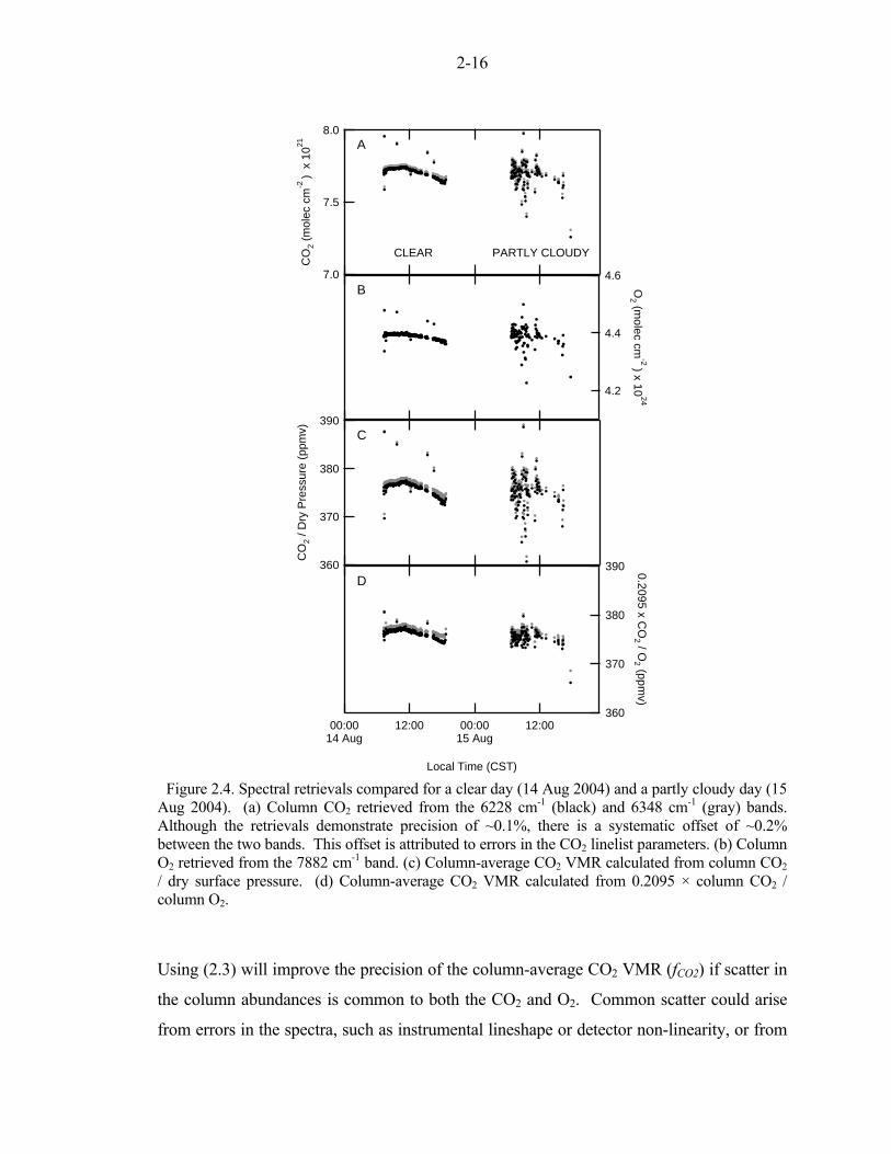
2-16

390

380

370

360

CO

2 / D

ry P

ress

ure

(ppm

v) C

390

380

370

360

0.2095 x CO

2 / O2 (ppm

v)

00:0014 Aug

12:00 00:0015 Aug

12:00

Local Time (CST)

D

8.0

7.5

7.0

CO

2 (m

olec

cm

-2 )

x 10

21 A

CLEAR PARTLY CLOUDY

4.6

4.4

4.2

O2 (m

olec cm-2 ) x 10

24

B

Figure 2.4. Spectral retrievals compared for a clear day (14 Aug 2004) and a partly cloudy day (15 Aug 2004). (a) Column CO2 retrieved from the 6228 cm-1 (black) and 6348 cm-1 (gray) bands. Although the retrievals demonstrate precision of ~0.1%, there is a systematic offset of ~0.2% between the two bands. This offset is attributed to errors in the CO2 linelist parameters. (b) Column O2 retrieved from the 7882 cm-1 band. (c) Column-average CO2 VMR calculated from column CO2 / dry surface pressure. (d) Column-average CO2 VMR calculated from 0.2095 × column CO2 / column O2.

Using (2.3) will improve the precision of the column-average CO2 VMR (fCO2) if scatter in

the column abundances is common to both the CO2 and O2. Common scatter could arise

from errors in the spectra, such as instrumental lineshape or detector non-linearity, or from

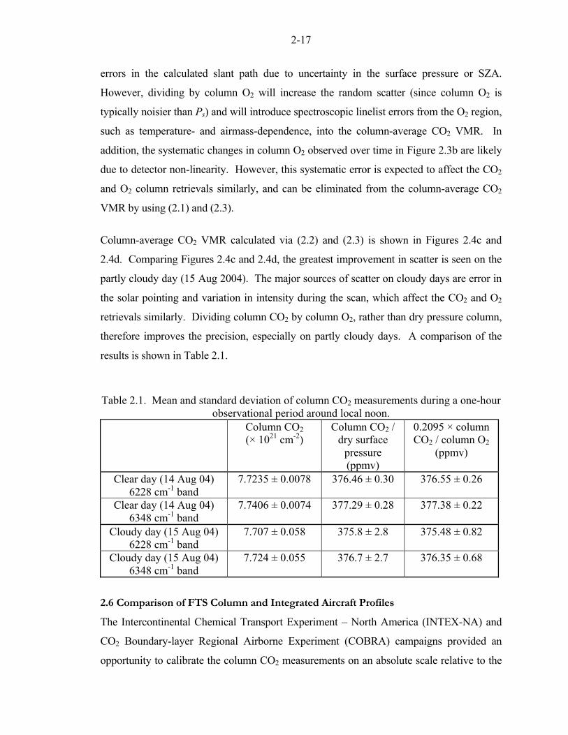
2-17

errors in the calculated slant path due to uncertainty in the surface pressure or SZA.

However, dividing by column O2 will increase the random scatter (since column O2 is

typically noisier than Ps) and will introduce spectroscopic linelist errors from the O2 region,

such as temperature- and airmass-dependence, into the column-average CO2 VMR. In

addition, the systematic changes in column O2 observed over time in Figure 2.3b are likely

due to detector non-linearity. However, this systematic error is expected to affect the CO2

and O2 column retrievals similarly, and can be eliminated from the column-average CO2

VMR by using (2.1) and (2.3).

Column-average CO2 VMR calculated via (2.2) and (2.3) is shown in Figures 2.4c and

2.4d. Comparing Figures 2.4c and 2.4d, the greatest improvement in scatter is seen on the

partly cloudy day (15 Aug 2004). The major sources of scatter on cloudy days are error in

the solar pointing and variation in intensity during the scan, which affect the CO2 and O2

retrievals similarly. Dividing column CO2 by column O2, rather than dry pressure column,

therefore improves the precision, especially on partly cloudy days. A comparison of the

results is shown in Table 2.1.

Table 2.1. Mean and standard deviation of column CO2 measurements during a one-hour

observational period around local noon. Column CO2

(× 1021 cm-2) Column CO2 /

dry surface pressure (ppmv)

0.2095 × column CO2 / column O2

(ppmv)

Clear day (14 Aug 04) 6228 cm-1 band

7.7235 ± 0.0078 376.46 ± 0.30 376.55 ± 0.26

Clear day (14 Aug 04) 6348 cm-1 band

7.7406 ± 0.0074 377.29 ± 0.28 377.38 ± 0.22

Cloudy day (15 Aug 04) 6228 cm-1 band

7.707 ± 0.058 375.8 ± 2.8 375.48 ± 0.82

Cloudy day (15 Aug 04) 6348 cm-1 band

7.724 ± 0.055 376.7 ± 2.7 376.35 ± 0.68

2.6 Comparison of FTS Column and Integrated Aircraft Profiles

The Intercontinental Chemical Transport Experiment – North America (INTEX-NA) and

CO2 Boundary-layer Regional Airborne Experiment (COBRA) campaigns provided an

opportunity to calibrate the column CO2 measurements on an absolute scale relative to the

2-18

standardized network of in situ measurements. As the difference between CO2 6228 cm-1

and 6348 cm-1 column retrievals in Figure 2.4a demonstrates, results from each of the CO2

bands are precise, but not sufficiently accurate. This is attributed to remaining limitations

in the available spectroscopic parameters.

The NASA DC-8 and University of Wyoming King Air measured in situ CO2 during

profiles over the WLEF Tall Tower site during summer 2004, using well-calibrated, mature

in situ CO2 sensors. Onboard the DC-8, dry CO2 VMR was measured at 1 Hz using a

modified LI-COR model 6252 infrared gas analyzer [Vay et al., 2003; Anderson et al.,

1996]. In-flight calibrations were performed at 15 minute intervals using standards

traceable to the WMO Central CO2 Laboratory. Onboard the King Air, similar 1 Hz

measurements were performed using a modified LI-COR model 6251 [Daube et al., 2002].

In-flight calibrations were performed with standards traceable to the Carbon Dioxide

Research Group at the Scripps Institute of Oceanography and NOAA ESRL. In-flight

calibrations show that the typical long term flight-to-flight precision of this technique is

better than ±0.1 ppmv [Daube et al., 2002].

The aircraft CO2 profiles can be integrated with respect to pressure for direct comparison

with FTS column CO2. Mathematically, this is found by combining the definition of the

column integral

(2.4)

with the hydrostatic equation

(2.5)

ngmdpdzair

−=

∫∞

=Zs

COCO dznfcolumn22

2-19

to yield

(2.6)

where f is the atmospheric mixing ratio, g is gravitational acceleration, m is molecular

mass, n is the number density, p is pressure, Ps is surface pressure, z is height, and Zs is the

surface height. The atmospheric mixing ratio of CO2 is defined as

(2.7)

where fCO2dry is the dry-air CO2 vmr, measured by in-situ instruments. Combining equations

(2.6) and (2.7) gives

(2.8)

Integrated column CO2 from (2.8) can be divided by the total column from (2.2) to yield

the column-average CO2 VMR.

Eight unique aircraft profiles were measured on five dates during 2004: 12 Jul, 14 Jul, 15

Jul, 14 Aug, and 15 Aug. The first profile of the series, shown in Figure 2.5a, was a

descending spiral by the NASA DC-8 from 10.0 km to 0.7 km. Because the aircraft has a

limited altitude range, it is necessary to make assumptions about CO2 and H2O in the upper

troposphere and stratosphere when using (2.8) to find integrated column CO2. The

)1(222 , OHdryCOCO fff −=

dp

ff

mm

gm

fcolumn

Ps

OH

OH

dryair

OHdryair

dryCOCO ∫

⎟⎟

⎠

⎞

⎜⎜

⎝

⎛⎟⎟⎠

⎞⎜⎜⎝

⎛

−+

=0

,,

,

2

22

2

2

11

∫=Ps

air

COCO dp

gmf

column0

2

2

2-20

tropopause pressure is determined from the NOAA CDC assimilated temperature profile.

The median CO2 value measured in the free troposphere is assumed to extend from the

aircraft ceiling to the tropopause. Above the tropopause, the assumed CO2 profile is taken

from an in situ balloon profile (35 N, 104 W) recorded over Fort Sumner, New Mexico

during September 2004. The balloon profile of CO2 as a function of altitude is coordinate-

transformed into CO2 as a function of potential temperature (θ), using simultaneous

temperature and pressure measurements. For the aircraft profile, θ is calculated from the

NOAA CDC assimilated temperature data. CO2 is assumed to be well-mixed in the

planetary boundary layer between the surface and the 0.7 km floor of the aircraft profile.

This is confirmed by in situ measurements on the Tall Tower. The CO2 profile shown in

Figure 2.5b is integrated with respect to pressure to find column CO2. The assumed CO2

profile above the aircraft ceiling contributes the greatest uncertainty to the integration, and

we have attributed a generous uncertainty of ±2 ppmv to this portion of the profile.

Figure 2.5d shows the FTS column-average CO2 recorded during a two-hour period which

brackets the aircraft profile. These profiles were performed at airmass 1.1 – 2.0 (SZA 25 –

60 deg). The column data is not continuous, because intermittent cloud prevented the

acquisition of solar spectra. The 45-minute period of the aircraft profile is indicated. The

averaging kernel for the FTS CO2 retrievals during this period is shown in Figure 2.5c.

The shape of the averaging kernel is typical for a uniformly mixed, moderately strong

absorber fitted by a non-linear least-squares profile-scaling retrieval. To accurately

compare the FTS column-average CO2 and integrated aircraft profile, it is necessary to

weight the aircraft profile by the FTS averaging kernel [Rodgers and Connor, 2003].

Because the averaging kernel varies slightly with airmass, a separate averaging kernel is

calculated for each aircraft overpass.

2-21

Figure 2.5. (a) Ground track of the NASA DC-8 during a vertical profile from 0.7 – 10.0 km on 12 Jul 2004. The location of the Wisconsin Tall Tower is indicated. Aircraft altitude is shown in color, where red = 0 km and purple = 12 km. (b) In situ CO2 measured during the 12 Jul 2004 profile. Tropopause pressure is determined from the NOAA CDC reanalysis. Above the aircraft ceiling (10.0 km), the median measured free tropospheric CO2 value is assumed to extend to the tropopause. Above the tropopause, the assumed CO2 profile is taken from a Sept 2004 balloon profile from 35 N, 104 W. The CO2 profile is integrated with respect to pressure to calculate the total column. (c) Averaging kernel for the FTS CO2 retrievals. (d) Column-averaged CO2 VMR for FTS spectra recorded during the aircraft profile. CO2 6228 cm-1 band retrievals shown in black; CO2 6228 cm-1 band retrievals shown in gray. Intermittent clouds prevented continuous data acquisition.

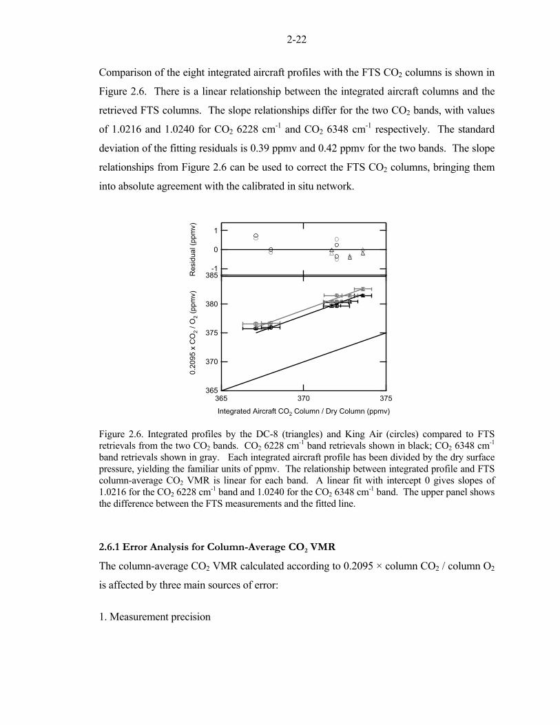
2-22

Comparison of the eight integrated aircraft profiles with the FTS CO2 columns is shown in

Figure 2.6. There is a linear relationship between the integrated aircraft columns and the

retrieved FTS columns. The slope relationships differ for the two CO2 bands, with values

of 1.0216 and 1.0240 for CO2 6228 cm-1 and CO2 6348 cm-1 respectively. The standard

deviation of the fitting residuals is 0.39 ppmv and 0.42 ppmv for the two bands. The slope

relationships from Figure 2.6 can be used to correct the FTS CO2 columns, bringing them

into absolute agreement with the calibrated in situ network.

��

��

��

��

��

��

��

��

��

�� !"�� #�$ � !"��

)*

�

*

+�'��"�!��

Figure 2.6. Integrated profiles by the DC-8 (triangles) and King Air (circles) compared to FTS retrievals from the two CO2 bands. CO2 6228 cm-1 band retrievals shown in black; CO2 6348 cm-1 band retrievals shown in gray. Each integrated aircraft profile has been divided by the dry surface pressure, yielding the familiar units of ppmv. The relationship between integrated profile and FTS column-average CO2 VMR is linear for each band. A linear fit with intercept 0 gives slopes of 1.0216 for the CO2 6228 cm-1 band and 1.0240 for the CO2 6348 cm-1 band. The upper panel shows the difference between the FTS measurements and the fitted line.

2.6.1 Error Analysis for Column-Average CO2 VMR

The column-average CO2 VMR calculated according to 0.2095 × column CO2 / column O2

is affected by three main sources of error:

1. Measurement precision

2-23

As discussed in Section 2.5, the standard deviation of column CO2 / column O2 during a

one hour period is better than 0.1% under clear sky conditions and ~0.2% under partly

cloudy conditions. Repeatability of the measurement is not a significant source of error.

2. Spectroscopic errors

As discussed in Section 2.5, the retrieved O2 columns were reduced by 2.27% to bring

them into agreement with the dry surface pressure. Although this correction falls outside

the reported uncertainty of the 16O16O 7882 cm-1 integrated band strength, we believe that it

is likely attributed to an error in the line strengths or air-broadened width parameters.

The absolute accuracy of the CO2 retrievals was calibrated by comparison to integrated

aircraft profiles, resulting in a correction of 1.0216 and 1.0240 for the CO2 6228 cm-1 and

6348 cm-1 bands. The standard deviation of the fitting residuals is 0.39 ppmv and 0.42

ppmv, or approximately 0.1%. The aircraft profiles were performed with the sun at airmass

1.1 – 2.0 (SZA 25 – 60 deg), and the column-average CO2 VMR is now well-calibrated for

these values. However, this does not calibrate the column-average CO2 VMRs at higher

airmass. A 1% change in the air-broadened widths results in a CO2 VMR change of ~0.2%

(±0.8 ppmv) at airmass 3 and ~0.6% (±2.3 ppmv) at airmass 12. These parameters are not

sufficiently constrained by current spectroscopic linelists, leaving this as a significant

source of systematic error which can be correlated with airmass, time of day, and

temperature.

3. Systematic instrumental changes over time

As described in Section 2.5, retrieved O2 VMR increased by ~0.3% during the observation

period. Because this increase is seen for O2 retrievals from the InGaAs detector in the 7882

cm-1 band, and not for O2 retrievals from the Si diode detector in the 13095 cm-1 A-band,

we believe that this is due to detector nonlinearity and can be corrected. We expect that

this error affects the CO2 and O2 retrievals similarly, but for now assume that the column

CO2 / column O2 ratio may also have a systematic error of 0.3% over the observation

period.

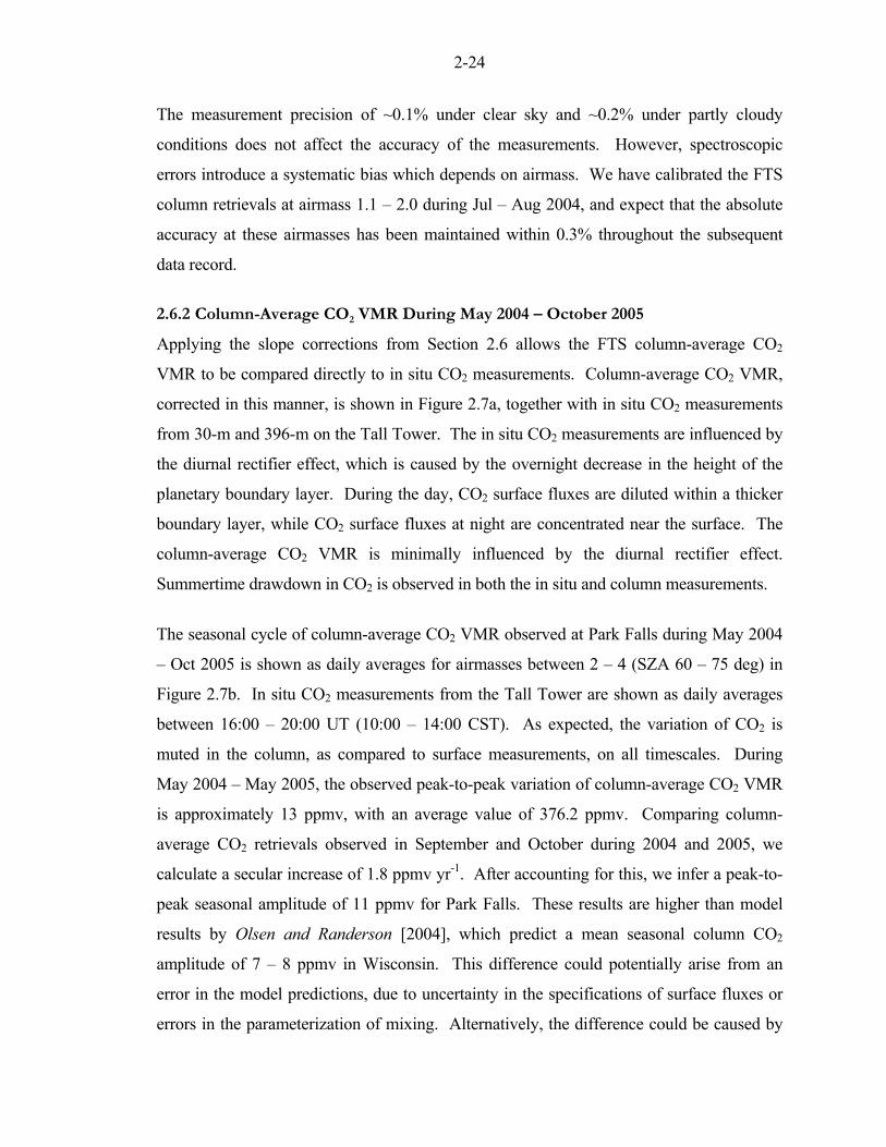
2-24

The measurement precision of ~0.1% under clear sky and ~0.2% under partly cloudy

conditions does not affect the accuracy of the measurements. However, spectroscopic

errors introduce a systematic bias which depends on airmass. We have calibrated the FTS

column retrievals at airmass 1.1 – 2.0 during Jul – Aug 2004, and expect that the absolute

accuracy at these airmasses has been maintained within 0.3% throughout the subsequent

data record.

2.6.2 Column-Average CO2 VMR During May 2004 – October 2005

Applying the slope corrections from Section 2.6 allows the FTS column-average CO2

VMR to be compared directly to in situ CO2 measurements. Column-average CO2 VMR,

corrected in this manner, is shown in Figure 2.7a, together with in situ CO2 measurements

from 30-m and 396-m on the Tall Tower. The in situ CO2 measurements are influenced by

the diurnal rectifier effect, which is caused by the overnight decrease in the height of the

planetary boundary layer. During the day, CO2 surface fluxes are diluted within a thicker

boundary layer, while CO2 surface fluxes at night are concentrated near the surface. The

column-average CO2 VMR is minimally influenced by the diurnal rectifier effect.

Summertime drawdown in CO2 is observed in both the in situ and column measurements.

The seasonal cycle of column-average CO2 VMR observed at Park Falls during May 2004

– Oct 2005 is shown as daily averages for airmasses between 2 – 4 (SZA 60 – 75 deg) in

Figure 2.7b. In situ CO2 measurements from the Tall Tower are shown as daily averages

between 16:00 – 20:00 UT (10:00 – 14:00 CST). As expected, the variation of CO2 is

muted in the column, as compared to surface measurements, on all timescales. During

May 2004 – May 2005, the observed peak-to-peak variation of column-average CO2 VMR

is approximately 13 ppmv, with an average value of 376.2 ppmv. Comparing column-

average CO2 retrievals observed in September and October during 2004 and 2005, we

calculate a secular increase of 1.8 ppmv yr-1. After accounting for this, we infer a peak-to-

peak seasonal amplitude of 11 ppmv for Park Falls. These results are higher than model

results by Olsen and Randerson [2004], which predict a mean seasonal column CO2

amplitude of 7 – 8 ppmv in Wisconsin. This difference could potentially arise from an

error in the model predictions, due to uncertainty in the specifications of surface fluxes or

errors in the parameterization of mixing. Alternatively, the difference could be caused by

2-25

differences between the assumed meteorology and emission inventories included in the

MATCH model.

��

��

��

��

��

��

��

��

��

��

�

��

��

��

��

��

��

�! �� "�# �� ! ��

$�%�

&

Figure 2.7. (a) Diurnal variation of column-average CO2 VMR (black) and Tall Tower CO2 at 30-m (red) and 396-m (blue). (b) Seasonal cycle of column-average CO2 VMR and Tall Tower CO2 during May 2004 – Oct 2005. Tall Tower CO2 is shown as daily averages between 10:00 – 14:00 CST. Column-average CO2 VMR is shown as daily averages for airmasses 2 – 4 (SZA 60 – 75 deg).

2.6.3 Conclusions

We have deployed an automated solar observatory to Park Falls, Wisconsin. Near-infrared

solar absorption spectra have been acquired continuously since May 2004. Short-term and

long-term precision are evaluated by the repeatability of column retrievals within a day and

by the comparison of column O2 with surface pressure measurements. The precision of

2-26

retrieved column CO2 under clear-sky conditions is ~0.1%, as determined by the 1σ

variability of retrievals recorded within one hour. Under partly cloudy conditions, the CO2

column precision is much worse, but can be improved by dividing column CO2 by column

O2 to calculate column-average CO2 VMR. This calculation eliminates errors which are

common to both CO2 and O2 retrievals, such as errors in solar pointing and variation in

solar intensity during interferogram acquisition, and allows useful retrievals to be obtained

under partly cloudy conditions. Comparison of retrieved column O2 to dry surface pressure

during May 2004 – October 2005 shows linear agreement with a 2.27 ± 0.25% bias.

The column CO2 retrievals were calibrated using aircraft profiles from the INTEX-NA and

COBRA campaigns during summer 2004. The CO2 6228 cm-1 and CO2 6348 cm-1 band

retrievals over-estimate the integrated aircraft profiles by factors of 1.0216 and 1.0240

respectively, with standard deviation of the fitting residuals of 0.39 ppmv and 0.42 ppmv.

The systematic differences are attributed to known uncertainty in the CO2 spectroscopic

linestrengths and air-broadened width parameters. The comparison to aircraft integrated

columns allows the CO2 6228 cm-1 and CO2 6348 cm-1 retrievals to be corrected to the

accepted in situ calibration scale. The aircraft profiles were performed with the sun at

airmass 1.1 – 2.0, and we are confident that our column-average CO2 VMRs are now well-

calibrated for these summertime, low airmass values. After calibration of the column

retrievals with the integrated aircraft profiles and consideration of the complete error

budget, we calculate the uncertainty in retrieved column-average CO2 VMR to be ~0.3%

(±1.1 ppmv) at airmasses less than 2 (SZA less than 60 deg) throughout the measurement

timeseries.

2.7 Acknowledgements

We thank Jeffrey Ayers for maintaining the ground-based FTS laboratory in Park Falls,

Wisconsin. We thank Arlyn Andrews and the NOAA CCGG for providing WLEF Tall

Tower CO2 measurements. Bruce Daube thanks Victoria Chow and Bhaswar Sen for their

support in obtaining the balloon CO2 profile. We thank Andrew Orr-Ewing for helpful

discussions and providing PGOPHER model results for the O2 7882 cm-1 band. R.A.W.

acknowledges support from the National Science Foundation and the California Institute of

Technology. This work was funded by NASA Grant NAG5-12247 and NNG05-GD07G.

2-27

Research at the Jet Propulsion Laboratory, California Institute of Technology is performed

under contract with NASA.

2.8 References

Anderson, B. E., G. L. Gregory, J. E. Collins, G. W. Sachse, T. J. Conway, and G. P.

Whiting (1996), Airborne observations of spatial and temporal variability of

tropospheric carbon dioxide, J. Geophys. Res., 101, 1985-1997.

Bakwin, P. S., P. P. Tans, B. B. Stephens, S. C. Wofsy, C. Gerbig, and A. Grainger (2003),

Strategies for measurement of atmospheric column means of carbon dioxide from

aircraft using discrete sampling, J. Geophys. Res., 108, doi:10.1029/2002JD003306.

Bakwin, P. S., P. P. Tans, C. L. Zhao, W. Ussler, and E. Quesnell (1995), Measurements of

carbon dioxide on a very tall tower, Tellus, 47, 535-549.

Berger, B. W., K. J. Davis, C. X. Yi, P. S. Bakwin, and C. L. Zhao (2001), Long-term

carbon dioxide fluxes from a very tall tower in a northern forest: Flux measurement

methodology, J. Atmos. Ocean. Tech., 18, 529-542.

Brault, J. W. (1996), New approach to high-precision Fourier transform spectrometer

design, Appl. Opt., 35, 2891-2896.

Cheah, S. L., Y. P. Lee, and J. F. Ogilvie (2000), Wavenumbers, strengths, widths and

shifts with pressure of lines in four bands of gaseous 16O2 in the systems a1Δ g - X3 Σg-

and b1Σg+ - X3 Σg

-, J. Quant. Spectrosc. Radiat. Transfer, 64, 467-482.

Daube, B. C., K. A. Boering, A. E. Andrews, and S. C. Wofsy (2002), A high-precision

fast-response airborne CO2 analyzer for in situ sampling from the surface to the middle

stratosphere, J. Atmos. Ocean. Tech., 19, 1532-1543.

Davis, K. J., P. S. Bakwin, C. X. Yi, B. W. Berger, C. L. Zhao, R. M. Teclaw, and J. G.

Isebrands (2003), The annual cycles of CO2 and H2O exchange over a northern mixed

forest as observed from a very tall tower, Glob. Change Biol., 9, 1278-1293.


Colello, and D. A. Dazlich (1996), Simulations of terrestrial carbon metabolism and


521-542.

2-28



doi:10.1029/2003JD004469.




edited.

Gloor, M., S. M. Fan, S. Pacala, and J. Sarmiento (2000), Optimal sampling of the

atmosphere for purpose of inverse modeling: A model study, Glob. Biogeochem. Cy.,

14, 407-428.






Nature, 415, 626-630.

Komhyr, W. D., R. H. Gammon, T. B. Harris, L. S. Waterman, T. J. Conway, W. R.

Taylor, and K. W. Thoning (1985), Global atmospheric CO2 distribution and variations

from 1968-1982 NOAA GMCC CO2 flask sample data, J. Geophys. Res., 90, 5567-

5596.

Kurylo, M. J., and S. Solomon (1990), Network for the Detection of Stratospheric Change,

NASA Report, Code EEU.

Lafferty, W. J., A. M. Solodov, C. L. Lugez, and G. T. Fraser (1998), Rotational

linestrengths and self-pressure-broadening coefficients for the 1.27-μm, a 1Δg - X3 Σg-, v

= 0-0 band of O2, Appl. Opt., 37, 2264-2270.

Newman, S. M., I. C. Lane, A. J. Orr-Ewing, D. A. Newnham, and J. Ballard (1999),

Integrated absorption intensity and Einstein coefficients for the O2 a1Δg - X3Σg

- (0,0)

transition: A comparison of cavity ringdown and high resolution Fourier transform

spectroscopy with a long-path absorption cell, J. Chem. Phys., 110, 10749-10757.

2-29

Newman, S. M., A. J. Orr-Ewing, D. A. Newnham, and J. Ballard (2000), Temperature and

pressure dependence of linewidths and integrated absorption intensities for the O2 a1Δg

- X3Σg- (0,0) transition, J. Phys. Chem., 104, 9467-9480.



doi:10.1029/2003JD003968.



213-232.



Rodgers, C. D., and B. J. Connor (2003), Intercomparison of remote sounding instruments,

J. Geophys. Res., 108, doi:10.1029/2002JD002299.

Rothman, L. S., D. Jacquemart, A. Barbe, D. C. Benner, M. Birk, L. R. Brown, M. R.

Carleer, C. Chackerian, K. Chance, L. H. Coudert, V. Dana, V. M. Devi, J. M. Flaud,

R. R. Gamache, A. Goldman, J. M. Hartmann, K. W. Jucks, A. G. Maki, J. Y. Mandin,

S. T. Massie, J. Orphal, A. Perrin, C. P. Rinsland, M. A. H. Smith, J. Tennyson, R. N.

Tolchenov, R. A. Toth, J. Vander Auwera, P. Varanasi, and G. Wagner (2005), The

HITRAN 2004 molecular spectroscopic database, J. Quant. Spectrosc. Radiat.

Transfer, 96, 139-204.

Smith, K. M., and D. A. Newnham (2000), Near-infrared absorption cross sections and

integrated absorption intensities of molecular oxygen (O2, O2-O2, and O2-N2), J.

Geophys. Res., 105, 7383-7396.

Smith, K. M., D. A. Newnham, and R. G. Williams (2001), Collision-induced absorption of

solar radiation in the atmosphere by molecular oxygen at 1.27 μm: Field observations

and model calculations, J. Geophys. Res., 106, 7541-7552.

Tans, P. P., I. Y. Fung, and T. Takahashi (1990), Observational Constraints on the Global

Atmospheric CO2 Budget, Science, 247, 1431-1438.

Vay, S. A., J. H. Woo, B. E. Anderson, K. L. Thornhill, D. R. Blake, D. J. Westberg, C. M.

Kiley, M. A. Avery, G. W. Sachse, D. G. Streets, Y. Tsutsumi, and S. R. Nolf (2003),

2-30

Influence of regional-scale anthropogenic emissions on CO2 distributions over the

western North Pacific, J. Geophys. Res., 108, doi:10.1029/2002JD003094.




doi:10.1029/2004GL021597.

Yang, Z., P. O. Wennberg, R. P. Cageao, T. J. Pongetti, G. C. Toon, and S. P. Sander

(2005), Ground-based photon path measurements from solar absorption spectra of the

O2 A-band, J. Quant. Spectrosc. Radiat. Transfer, 90, 309-321.



doi:10.1029/2001GL014537.

Zhao, C. L., P. S. Bakwin, and P. P. Tans (1997), A design for unattended monitoring of

carbon dioxide on a very tall tower, J. Atmos. Ocean. Tech., 14, 1139-1145.

3-1

Chapter 3

SURFACE EXCHANGE OF CO2 OBSERVED BY COINCIDENT

EDDY COVARIANCE FLUX AND COLUMN MEASUREMENTS*

3.1 Abstract

Measurements of column CO2 at the WLEF Tall Tower site in Northern Wisconsin are

used to calculate CO2 exchange on seasonal and daily timescales. Comparisons of column

and in situ measurements confirm model predictions that the column measurements are

representative of Northern Hemispheric CO2 exchange over seasonal timescales.

TransCom 3 models underpredict the seasonal cycle observed in the column measurements,

suggesting that the Carnegie-Ames-Stanford Approach (CASA) terrestrial biosphere model

may underestimate the magnitude of the growing season net flux. The precision of the

column measurements (~0.1%) is sufficient to directly infer daytime fluxes from the

temporal gradient of the CO2 column. Net ecosystem exchange is calculated from the

column abundance of CO2 and compared with eddy covariance measurements. Although

the observation of net ecosystem exchange in the column is obscured by concentration

changes due to transport, the column and eddy covariance measurements agree when

averaged seasonally.

3.2 Introduction

The atmospheric abundance of CO2 has increased from 280 ppmv in pre-industrial times to

~370 ppmv in 1999, and continues to increase at a rate of 1 – 2 ppmv yr-1 [(IPCC), 2001].

This increase is attributed to fossil fuel consumption [Marland, 2000] and land use change

[Houghton, 1999]. The magnitude of the global release of CO2 from the burning of fossil

fuels is well known [Marland, 2000]. The discrepancy between this value and the mass of

CO2 accumulating in the atmosphere is attributed to uptake by oceans and the terrestrial

biosphere [Battle et al., 2000; Keeling et al., 1993; Keeling and Shertz, 1992].

3-2

Understanding the current and future carbon balance of the terrestrial biosphere is

important for predicting future atmospheric CO2 levels.

Top-down estimates of the magnitude of CO2 sources and sinks are currently inferred from

in situ measurements at two global networks of surface sites, operated by NOAA and the

Scripps Institute of Oceanography [GLOBALVIEW-CO2, 2005; Conway et al., 1994;

Keeling et al., 1995]. Studies combine these in situ measurements with global transport

models to estimate regional-scale surface exchange of CO2 using inversion techniques

[Gurney et al., 2002; Rayner et al., 1999; Tans et al., 1990]. This has proven difficult,

because although the measurements are highly accurate, they have limited spatial coverage

and are generally confined to the convective boundary layer. Because CO2 exchange and

changes in boundary layer height are correlated on diurnal and seasonal timescales, errors

in parameterization of diurnal and seasonal CO2 fluxes can be aliased into the inferred

exchange terms as “rectifier effects” [Denning et al., 1996a; Denning et al., 1995; Denning

et al., 1996b].

Integrated column measurements of CO2 have the potential to constrain top-down estimates

of carbon exchange. Because the column integral of CO2 is not influenced by diurnal

variations in the convective boundary layer, column measurements are not affected by the

seasonal and diurnal rectifier effect. In addition, column measurements sample a larger

portion of the atmosphere, which results in less spatial variability and less influence of local

sources and sinks, while retaining information about the regional surface fluxes. Olsen and

Randerson [2004] concluded that with a few high-precision observation sites, it would be

possible to assess the strength of the Northern Hemisphere carbon sink and that this

approach would be less sensitive to model representations of vertical mixing. Similarly,

Rayner and O’Brien [2001] observe that column-integrated data are less susceptible than

surface measurements to uncertainties in model transport.

Column measurements also have the potential to directly constrain bottom-up estimates of

CO2 exchange on diurnal timescales. Many of the same advantages that make the CO2

column a useful tool for atmospheric inversions, such as insensitivity to the rectifier effect,

also make it useful for directly quantifying regional CO2 exchange. However, because the

3-3

fluxes are inferred from the temporal gradient in the CO2 column, the column observations

must be highly precise. In addition, if changes in the column due to simple transport are

not sufficiently small or sufficiently well constrained, they will overwhelm the small

changes due to surface uptake.

The potential for column measurements to constrain both top-down and bottom-up

estimates of CO2 exchange is possible because the measurements simultaneously represent

two different spatial footprints, when considered over different time scales. The “footprint”

is defined as the contribution of each element of the upwind surface area to the measured

flux, and is synomous with the transfer function or source weighting function. Assuming a

mean windspeed of 10 m s-1 in the atmospheric boundary layer and free troposphere, the

change in column CO2 within a single 10-hr period represents a footprint length of ~360

km. Observations of daytime changes in CO2 can be used directly to infer fluxes for this

spatial region. Rapid mixing within the troposphere results in a much larger footprint over

longer timescales. The seasonal phase and amplitude of a column CO2 measurement is

approximately representative of the entire hemisphere, and model predictions show that the

seasonal amplitude of column CO2 will be similar at terrestrial and oceanic sites within the

same latitude band [Olsen and Randerson, 2004]. Overall, column measurements will

observe the hemispheric seasonal cycle, with daytime changes due to local sources and

sinks superimposed on the larger trend.

This work presents CO2 exchange on seasonal and daily timescales observed by column

measurements at a forested site in Northern Wisconsin. Near-infrared solar absorption

spectra can be used to determine the column abundance of CO2 and other greenhouse gases

[Yang et al., 2002; Washenfelder et al., 2006; Dufour et al., 2004; Warneke et al., 2005].

To evaluate carbon exchange on seasonal timescales, CO2 column measurements from

May 2004 – March 2006 are compared to in situ measurements and TransCom model

predictions. To examine carbon exchange on daily timescales, we compare column

measurements to eddy covariance measurements acquired in and above the convective

boundary layer. We calculate the daytime drawdown of CO2 observed by column and eddy

covariance measurements during short time periods (on the order of six hours) to evaluate

3-4

the spatial representativeness of these two datasets in observing CO2 net ecosystem

exchange (NEE).

3.3 Column Measurements: Instrumentation and Data Analysis

The column measurements described in this work were acquired at an automated

observatory located at the WLEF Tall Tower site in Northern Wisconsin. The observatory

was developed for highly precise, ground-based solar absorption spectrometry, and it is the

first dedicated observatory in the Total Carbon Column Observing Network (TCCON).

Solar tracking optics and a Fourier Transform Spectrometer (FTS) are used to record near-

infrared spectra of the sun at high spectral resolution. Solar spectra are acquired

continuously during clear sky conditions, with each spectrum requiring ~110 seconds.

Details regarding the FTS observatory and analysis technique can be found in

Washenfelder et al. [2006]. Measurement precision of ~0.1% is demonstrated for retrievals

of column CO2 and column O2 under clear-sky conditions [Washenfelder et al., 2006].

Column-average CO2 VMRs are calculated by ratioing column CO2 with surface pressure

or column O2. Column-average CO2 VMRs have been calibrated by comparison with

integrated aircraft profiles [Washenfelder et al., 2006].

3.4 Research Site

The FTS observatory is located 25 m south of the WLEF television tower (45.495 N,

90.273 W, 442 m) in the Park Falls Ranger District of the Chequamegon National Forest,

12 km east of Park Falls, Wisconsin, U.S.A. The Chequamegon National Forest was

extensively logged between 1860 and 1920, but has since regrown [Bakwin et al., 1998].

The Wisconsin Department of Natural Resources has employed LANDSAT Thematic

Mapper satellite imagery and ground truthing to assemble the Wisconsin Initiative for

Statewide Cooperation on Landscape Analysis and Data (WISCLAND) land cover map

[WiDNR, 1998]. The WISCLAND inventory shows that within a 10-km radius of WLEF,

82.4% of the landcover is classified as aspen, maple, sugar maple, and mixed deciduous

and coniferous forests, with an additional 1.4% classified as emergent and wetland

meadow, and 2.4% classified as open water. The deciduous species include aspen, birch,

maple, basswood, and alder. The coniferous species include balsam fir, red pine, jack pine,

3-5

��

��

��

��

�

��

��

��

��

�

�

�

��

��

�

��

��

��

��

��

��

��

��!��

��

��

��

"��#��

��

$��

%�&� ��

'�� (��

)��

��#

*��#

�� #

%��

+��,��

%�&� �� (��

%�&� ��

��

��

-,��,��

��.��

��

'�� (��

'�� (��

*�� (��

��

'�� (��

��

%�&� ��

'��

+��

�� #, ��

��

��

�

�� ' �� #, ��

Figure 3.1. (a) Wisconsin Initiative for Statewide Cooperation on Landscape Analysis and Data (WISCLAND) land cover classification map for the region surrounding the WLEF tower site [WiDNR, 1998]. (b) Landcover distribution within a 10-km and 100-km radius of the WLEF tower, demonstrating that the forest cover is roughly homogeneous.

black spruce, and white cedar. Within a 100-km radius of WLEF, 76.6% of the landcover

is similarly classified as aspen, oak, maple, sugar maple, and mixed deciduous and

coniferous forests, with 1.9% classified as emergent and wetland meadow, and 5.9%

3-6

classified as open water. Figure 3.1 shows a map of the study area and a histogram of the

WISCLAND landcover designations. Further details regarding landcover are given in the

literature [Burrows et al., 2002; Cook et al., 2004; Davis et al., 2003; MacKay et al., 2002].

3.5 Seasonal CO2 Exchange

3.5.1 Park Falls WLEF Site During 2004 – 2005

Column-average CO2 VMRs are shown together with in situ CO2 VMRs recorded at 396-m

on the WLEF tower in Figure 3.2. Qualitatively, column CO2 behaves similarly to surface

CO2, but is much more uniform spatially and temporally [Olsen and Randerson, 2004].

Daytime averages for the column-average CO2 measurements are calculated for solar

zenith angles (SZA) 60 deg – 75 deg (airmass 2 – 4) to minimize seasonal biases due to

SZA [see Washenfelder et al., 2006]. Daytime averages for the in situ measurements are

shown for 10:00 – 14:00 local standard time, to minimize seasonal bias due to the rectifier

effect. The column-average CO2 VMR is greater than the in situ mixing ratio at the top of

the tower during the summer and fall, but less in the winter and spring. This is consistent

with model predictions by Olsen and Randerson [2004] for column and surface

measurements at Northern Hemisphere mid-latitudes.

During May 2004 – March 2006, the observed peak-to-peak variation of column-average

CO2 at Park Falls is approximately 13 ppmv with an average value of 376.3 ppmv. With a

secular trend of 1.8 ppmv yr-1 observed in the column measurements, we infer a peak-to-

peak seasonal amplitude of 11 ppmv. This supports the prediction that column

measurements in the Northern Hemisphere will be generally representative of Northern

Hemispheric CO2 exchange over seasonal timescales [Olsen and Randerson, 2004].

Column measurments are acquired only under clear-sky conditions, and recent work shows

that this may introduce a difference of -0.2 to -0.4 ppmv compared to measurements under

all viewing conditions [Corbin and Denning, 2006]. The difference is predicted during

both summer and winter and is attributed to enhanced photosynthesis and changes in

advection during clear days. Considering this, we report the peak-to-peak seasonal

amplitude as 11 ppmv ± 1 ppmv.

3-7

��

��

��

��

��

��

��

�

��

��

��

�� !�"�

��# � $%%

Figure 3.2. CO2 and surface exchange observed at the WLEF Tall Tower site. Three independent datasets acquired at the WLEF Tall Tower site during 2004 – 2006 are shown. (i) Column-average CO2 measured by FTS (black; daily average for SZA 60 – 75 deg); (ii) In situ CO2 VMR at 396-m (red; daily average for 10:00 – 14:00 local standard time); (iii) Cumulative NEE (blue; gap-filled measurements of preferred NEE with constant offset of 380 ppmv).

The observed peak-to-peak seasonal amplitude at Park Falls is similar to the reported

amplitude of 11 ppmv observed at Spitsbergen, Norway (78.9 N, 11.9 E, 0.02 km above

sea level) during 2002 – 2004 [Warneke et al., 2005] and larger than the reported peak-to-

peak seasonal amplitude of ~7 ppmv observed at the Kitt Peak National Solar Observatory

(31.9 N, 111.6 W, 2.09 km above sea level) during 1977 – 1995 [Yang et al., 2002].

However, it is difficult to draw further conclusions directly from comparing the seasonal

amplitude at Park Falls, Spitsbergen, and Kitt Peak. As a mountain site, Kitt Peak is

affected by convective mixing that may vary diurnally and seasonally. Wintertime

measurements at Spitsbergen are recorded at high SZA, and this may introduce a seasonal

bias of a few ppmv, which has not yet been calibrated.

3.5.2 Comparison to TransCom Model Predictions

The Atmospheric Tracer Transport Model Intercomparison Project (TransCom) is an

intercomparison of transport models used to calculate the size and distribution of regional

carbon fluxes by inverting in situ measurements. The TransCom 3 experiment included 16

different transport model and model variants that differ in spatial resolution, advection

scheme, driving winds, and sub-grid scale parameterizations [Gurney et al., 2002; Gurney

3-8

et al., 2003]. For the TransCom 3 comparison, these transport models were initialized

identically with a standard set of background fluxes that included fossil fuel emission

fields, an annually-balanced terrestrial biosphere, and air-sea gas exchange [Gurney et al.,

2002; Gurney et al., 2003]. The seasonal biosphere exchange (1 deg x 1 deg) was derived

from the Carnegie-Ames-Stanford Approach (CASA) terrestrial biosphere model

[Randerson et al., 1997], and has an annual total flux of zero at every grid cell. The

background fossil fuel fluxes were prescribed without seasonality. In the current work, we

have adopted the TransCom 3 experimental protocol, but have scaled the 1995 fossil fuel

emission inventory by 1.10 to better represent 2004 – 2006.

The TransCom 3 model predictions of the CO2 seasonal cycle for the 925 mb pressure

surface and the total column at the WLEF site are shown in Figure 3.3. Horizontal

resolution varies between the models, but is typically on the order of 3 deg × 3 deg.

Because the total atmospheric mass of CO2 in the different models is essentially identical,

the range in the model prediction is mainly due to differences in the assumed

meteorological wind fields and the representation of atmospheric mixing processes, such as

convection. The observed seasonal amplitude in the column significantly exceeds both the

average TransCom model prediction and the range of predictions, suggesting that the error

is not due to transport.

Yang et al. [2006, in preparation] analyze the TransCom models together with aircraft

profiles, and conclude that (i) the models do not accurately represent the mixing of the

planetary boundary layer with the free troposphere (on average they are too stratified); and

(ii) a small number of additional measurements in the free troposphere could constrain the

models, resulting in more accurate partitioning of inter-hemispheric carbon fluxes. The

column measurements provide additional diagnostic information for evaluating the

TransCom models. Although they lack the profile information that is available from

aircraft measurements, the column measurements are recorded continuously at higher

sampling frequency and have a larger seasonal footprint than the aircraft measurements.

The evidence in Figure 3.3 and the mid-tropospheric aircraft data analyzed by Yang et al.

[2006, in preparation] consistently suggests that vertical mixing is under-represented in the

3-9

TransCom models. This explanation would also resolve differences between the measured

and modeled seasonal cycle of column CO2 at the Kitt Peak National Solar Observatory

[Olsen and Randerson, 2004]. Because the TransCom 3 models are able to reproduce

measurements of surface CO2, whilc underestimating the vertical mixing, this suggests that

the seasonal variation of NEE in the Northern Hemisphere is underestimated by the CASA

neutral biosphere.

-30

-20

-10

0

10

20

30

CO

2 VM

R (p

pmv)

-8

-4

0

4

8

Col

umn-

Aver

age

CO

2 VM

R (p

pmv)

Jan Mar May Jul Sep NovDate

Figure 3.3. (a) TransCom model results for the 925 mb pressure level for the gridbox containing the WLEF Tall Tower site (solid line represents average; grey lines show range of model predictions). Detrended in situ CO2 VMR measurements from 396-m (daily average for 10:00 – 14:00 local standard time) are also shown (black circles). The trend and annual mean have been subtracted from each dataset. (b) Column-average CO2 VMRs (black circles) for May 2004 – March 2006 are shown with integrated TransCom vertical profiles (solid line represents average; grey lines show range of model predictions). Each of the TransCom models underpredict the seasonal cycle observed in the column measurements.

3.6 Local CO2 Exchange

3.6.1 Bottom-Up Estimates of Local CO2 Exchange.

In contrast to the top-down approach of atmospheric inversions, the bottom-up approach

attempts to scale-up direct measurements of CO2 exchange on local scales to constrain the

3-10

global carbon budget. Here, we evaluate the potential of column measurements at the

WLEF site for constraining estimates of local NEE and compare these measurements to

eddy covariance measurements recorded on the WLEF tower. The main challenge in

inferring fluxes from a concentration gradient is that this requires that the column changes

due to transport are either small or can be modeled. An additional impediment is that the

column measurements are only possible when the sun is unobscured by clouds, meaning

that continuous measurements are not available.

Eddy covariance measurements have been used successfully to quantify CO2 exchange on

local scales. The eddy covariance method is a statistical technique used to analyze high

frequency wind and scalar atmospheric data to determine the vertical flux of trace gases

[Baldocchi, 2003]. The eddy covariance method provides a direct measure of CO2 surface

exchange, and allows NEE to be assessed at the level of an entire ecosystem over

timescales of hours to years [Baldocchi et al., 1988; Goulden et al., 1996; Wofsy et al.,

1993]. The footprint length is typically 10 – 100 times greater than the measurement

height and varies with meteorological conditions, falling in the range of hundreds of meters

to tens of kilometers depending on the height of the tower. The method is most applicable

over flat terrain, under steady environmental conditions, and with homogeneous vegetation

for an extended distance upwind. Ignoring these constraints can introduce systematic

errors in interpretation. In addition, diurnal changes in footprint area can introduce

difficulty in calculating temporally-integrated NEE [Wang, 2005].

Understanding the spatial representativeness of eddy covariance measurements is a

challenge. Measured fluxes may not be broadly representative of different ecosystem

classifications due to differences in canopy age, canopy density, tree roots, soil, litter

quality, plant species, micrometeorological conditions, and other biological factors [Wang,

2005]. A recent study by Wang [2005] of eddy covariance observations in and around Park

Falls shows that a simple ecosystem classification system cannot capture the variability of

CO2 NEE between different ecosystems. Wang concludes that no small flux tower can

accurately represent regional CO2 exchange [Wang, 2005].

3-11

3.6.2 Eddy Covariance: Instrumentation and Data Analysis

Fluxes of CO2, water vapor, virtual temperature, and momentum are measured

continuously at 30, 122, and 396 m on the WLEF tower. CO2 and water vapor mixing

ratios are measured using infrared gas analyzers (Li-Cor Inc., Lincoln, Nebraska, model LI-

6262). Virtual temperature and momentum are measured using sonic anemometers

(Applied Technologies Inc., Boulder, Colorado, model SATI/3K or Campbell Scientific

Inc., Logan, Utah, model CSAT3). High-precision, high-accuracy CO2 mixing ratio

measurements are simultaneously recorded at 11, 30, 76, 122, 244, and 396 m using two

Li-Cor model LI-6251 infrared gas analyzers [Bakwin et al., 1998; Zhao et al., 1997].

These measurements are used to calibrate the fast-response infrared gas analyzers and to

calculate the rate of change of storage for CO2 [Davis et al., 2003]. The eddy covariance

instrumentation and methodology is described in detail in Berger et al. [2001] and Davis et

al. [2003].

NEE is the net flux of carbon from the surface and can be described as the sum of the

turbulent flux at the measured height plus the rate of change of CO2 mass in the atmosphere

below. Studies conducted at the WLEF site conclude that the horizontal and vertical

advection terms make a negligible contribution to daytime NEE [Wang et al., 2005; Yi et

al., 2000]. Previous work has examined the long-term average of NEE at the three

observation levels of the WLEF tower [Davis et al., 2003], with consideration of the

measurement footprint under varying conditions of convective mixing. The authors

developed an algorithm for “preferred” NEE that combines measurements at the three

levels to maintain a large footprint while avoiding the influence of the clearing around the

tower. Preferred NEE has been adopted for this comparison.

3.6.3 Calculation of Net Ecosystem Exchange from the Total Column

Column and eddy covariance measurements of CO2 can each be used to calculate NEE.

However, the total observed change in the column CO2 abundance includes changes due to

NEE, surface pressure, and transport (horizontal advection in the convective boundary

layer and free troposphere). Transport will alter the vertical column of CO2 if regional

gradients exist in the concentration field.

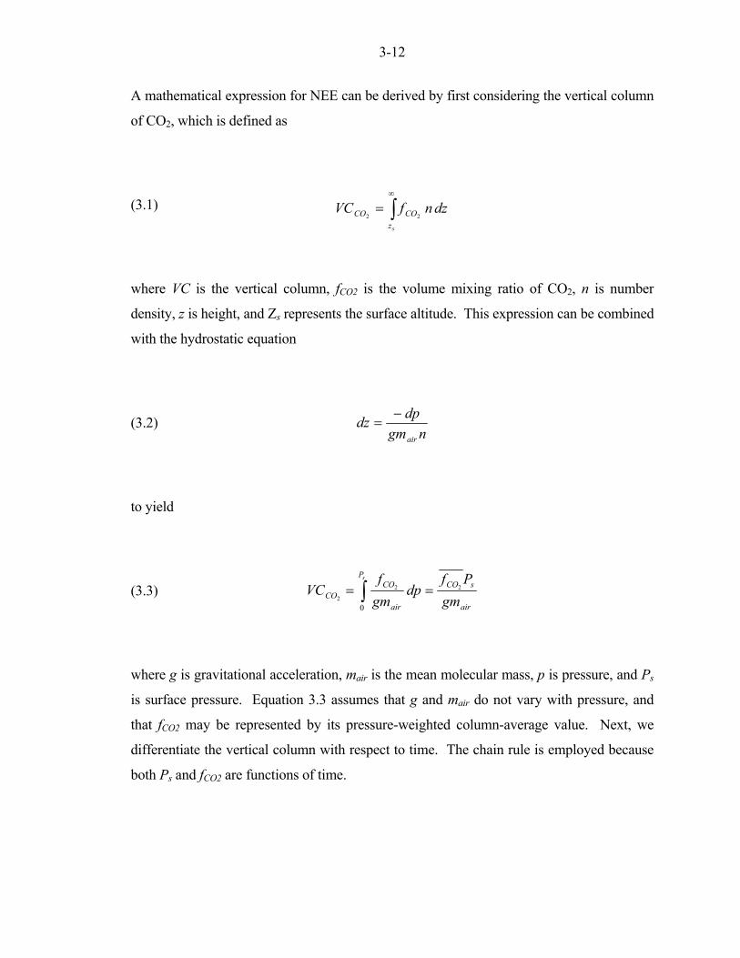
3-12

A mathematical expression for NEE can be derived by first considering the vertical column

of CO2, which is defined as

(3.1)

where VC is the vertical column, fCO2 is the volume mixing ratio of CO2, n is number

density, z is height, and Zs represents the surface altitude. This expression can be combined

with the hydrostatic equation

(3.2)

to yield

(3.3)

where g is gravitational acceleration, mair is the mean molecular mass, p is pressure, and Ps

is surface pressure. Equation 3.3 assumes that g and mair do not vary with pressure, and

that fCO2 may be represented by its pressure-weighted column-average value. Next, we

differentiate the vertical column with respect to time. The chain rule is employed because

both Ps and fCO2 are functions of time.

∫∞

=sz

COCO dznfVC22

ngmdpdzair

−=

air

sCOP

air

COCO gm

Pfdp

gmf

VCs

22

2

0

== ∫

3-13

(3.4)

Equation 3.4 can be further simplified by introducing the vertical column of O2, which the

FTS observes simultaneously in the near-infrared solar spectra. O2 is well-mixed in the

atmosphere, with a dry-air volume mixing ratio of 0.2095. The vertical column of O2 can

be expressed as

(3.5)

Substituting Equations 3.3 and 3.5 into Equation 3.4 gives a complete expression for the

observed change in VCCO2 with time, which includes contributions from NEE, change in

surface pressure, and transport:

(3.6)

The first term on the LHS of Equation 3.6 represents the total observed change in the

column. The second term on the LHS of Equation 3.6 represents the change in VCCO2 due

to changes in the surface pressure, with the assumption that the change in fCO2 is negligible

with respect to the change in surface pressure. The change in column CO2 due to surface

pressure is typically negative during the day, due to the diurnal and semidiurnal pressure

tides. The tides have annually-averaged magnitudes of 0.5 hPa and 0.4 hPa respectively,

with peaks at ~10:00 and ~9:00/21:00 local standard time [Dai and Wang, 1999]. The

RHS represents the change in VCCO2 due to both NEE and transport. It is difficult to

air

sOO gm

PfVC 2

2=

dtfd

fVC

dtdVC

ff

dtdVC CO

O

OO

O

COCO 2

2

22

2

22 =−

dtfd

f

VCdt

dPP

VCdt

dVC CO

CO

COs

s

COCO 2

2

222 +=

3-14

separate these two contributions, because they both alter the observed volume mixing ratio

of CO2.

Quantifying the change in CO2 due to transport in order to better calculate NEE represents

a challenge. Constraining this term would require a model capable of predicting regional

CO2 gradients of less than 1 ppmv over times scales of a many hours. Alternatively, a

tracer approach could be used to determine when the influence of transport is negligble.

CO is anthropogenic, with a moderate lifetime, no local flux, and a summertime latitudinal

gradient. However, we have found that the change in column CO is not well-correlated

with changes in column CO2 due to transport, which precludes the use of CO as a tracer. In

general, we expect that the change in VCCO2 due to transport is negligible when Equation

3.6 is employed over time periods of a few hours, but that this contribution becomes

significant over longer time periods. This work analyzes CO2 exchange on timescales

sufficiently short that transport may be neglected.

Although the precision of column CO2 retrievals is high, we observe systematic errors that

depend on SZA. As the observed optical path through the atmosphere increases with

increasing SZA, the optical depth of CO2 absorption lines increases. The error is attributed

to uncertainties in the spectroscopic linelist parameters used to calculate the absorption

coefficients. SZA-dependent errors can be introduced by errors in the air-broadened

linewidths, the temperature-dependence of the air-broadened linewidths, or the relative

strengths of lines with different lower state energies. A small change in the linelist

parameters, such as a 1% change in the air-broadened linewidths, will change column-

average CO2 VMR by ±0.4 ppmv at SZA 70 deg. Unfortunately, the existing laboratory

spectroscopy is insufficient to achieve our desired accuracy, and the aircraft profiles

previously used for calibration [Washenfelder et al., 2006] were not recorded during high

SZAs and can not be used to quantify this error.

For the analysis described in this work, we calculate Equation 3.6 symmetrically around

local solar noon (e.g. from [local solar noon – 2] hrs to [local solar noon + 2 hrs]). This

eliminates bias due to errors that depend on solar zenith angle, including most

spectroscopic errors.

3-15

3.6.4 Comparison of Drawdown Observed by FTS and Eddy Covariance

Figure 3.4 shows the drawdown observed during a sunny period in September 2004. The

plot shows eddy covariance measurements of NEE and FTS total column measurements

corrected by the surface pressure change (Equation 3.6), which represent changes in

column CO2 due to both NEE and transport. In each case, the measurements have been

integrated with respect to time, and the noontime average has been subtracted from each

24-hour period of data, so that the two datasets appear on a common scale centered at zero.

Some of the apparent drawdown observed in the FTS total column measurements is due to

systematic bias in the column at high SZA, and this illustrates the need to analyze the FTS

column data symmetrically around local solar noon, as described in Section 3.6.3.

Additionally, neglecting the transport term in Equation 3.6 introduces an error that varies

between days.

-0.5

0.0

0.5

DC

O2

( m

ol m

-2 )

9/8/04 9/9/04 9/10/04 9/11/04

Date Figure 3.4. Comparison of the drawdown observed during 8 Sept – 11 Sept 2004 in the eddy covariance and FTS total column measurements. The FTS total column measurements corrected by the change in surface pressure (Equation 3.6) are shown in green. The eddy covariance measurements of NEE are shown in black. The noontime average has been subtracted from each 24-hour period of data so that the measurements appear on a common scale around zero. Some of the overestimation of drawdown observed in the column measurements is due to systematic bias in the column retrievals at high solar zenith angles.

NEE calculated from the column measurements according to Equation 3.6, and separately

from the eddy covariance measurements is shown in Figures 3.5a and 3.5b. The change in

CO2 observed by the column measurements includes contributions from both NEE and

transport. As mentioned previously, we have analyzed differences in column CO2

symmetrically around local solar noon to minimize problems with SZA dependence of the

3-16

FTS column retrievals. Figure 3.5 shows the integrated change in column CO2 relative to

elapsed time around local solar noon (e.g. 4:00 represents the change from 2 hours before

local noon to 2 hours after local noon). If we assume that the column and eddy covariance

measurements have sufficiently similar footprints, then the difference between Figure 3.5a

and 3.5b will give an estimation of the transport term, as seen in Figure 3.5c.

-1.0

-0.5

0.0

0.5

DC

O2

Tran

spor

t ( m

ol m

-2 )

00:00 02:00 04:00 06:00 08:00 10:00 12:00

Elapsed Time

C

-1.0

-0.5

0.0

0.5

DC

O2

NE

E (

mol

m-2

)

B

-1.0

-0.5

0.0

0.5D

CO

2 FT

S To

tal -

Ps

( mol

m-2

)

A

Figure 3.5. Comparison of NEE calculated from eddy covariance and column measurements. The elapsed time represents the time difference around local noon (e.g. 4:00 represents the change from 2 hours before local noon to 2 hours after local noon). Day of year is shown in color, with January as red and December as purple. (a) Change in column CO2 observed by FTS measurements, calculated from Equation 3.6, including both NEE and transport. (b) Change in column CO2 due to NEE, as measured by eddy covariance. (c) The difference between (a) and (b) is attributed to transport of airmasses in the convective boundary layer and the free troposphere.

3-17

Figure 3.5c shows that, on average, the affect of transport is approximately neutral. Instead

of quantifying the contribution of transport in Equation 3.6, we assume that it will

introduce noise into our results, but will have no net contribution to the drawdown when

averaged over several days.

With this assumption, we directly compare the drawdown observed in the FTS total column

measurements and eddy covariance measurements during different seasons. The results are

shown in Figure 3.6. The FTS total column measurements corrected by the change in

surface pressure (Equation 3.6) and the eddy covariance measurements of NEE have been

integrated over a four-hour period around local noon each day. As expected, Figure 3.6a

shows significant variability in the drawdown observed by the FTS column measurements,

due to the neglect of the transport term in Equation 3.6. However, when the data is

averaged over seasonal timescales, the agreement is improved. This is consistent with the

hypothesis that horizontal CO2 gradients on average exert a neutral effect on the column.

Because the column measurements are biased to sunny conditions, only coincident eddy

covariance measurements of NEE are included in the seasonal average. The final panel of

Figure 3.6 shows the correlation between column and eddy covariance measurements of

CO2 drawdown. The differences between the two techniques may represent differences in

the measured footprint. Alternatively, if wind direction and regional CO2 gradients are

correlated seasonally, then the transport term may introduce a seasonal bias between the

column and eddy covariance measurements of NEE.

These results show that the column measurements are sufficiently precise to observe CO2

exchange. However, the results would be improved by better constraining changes in the

CO2 column due to transport.

3-18

-0.4

-0.2

0.0

0.2

DC

O2

Col

umn

( mol

m-2

)

-0.4 -0.2 0.0 0.2

DCO2 NEE ( mol m-2 )

C

-0.4

-0.2

0.0

0.2

1/04 4/04 7/04 10/04 1/05 4/05 7/05 10/05 1/06Date

B

-0.4

-0.2

0.0

0.2

DC

O2

( mol

m-2

)

A

Figure 3.6. (a) Drawdown observed by eddy covariance and total column measurements during a four-hour period bracketing local solar noon. The FTS total column measurements corrected by the change in surface pressure (Equation 3.6) are shown is green. The eddy covariance measurements of NEE are shown in black. (b) Seasonal average of measurements shown in (a). Because the column measurements are biased to sunny conditions, only coincident eddy covariance measurements of NEE are included in the seasonal average. Error bars represent the ±1σ standard deviation of the mean. (c) Correlation plot showing agreement between FTS total column measurements corrected by the change in surface pressure and eddy covariance measurements of NEE on seasonal timescales. 3.7 Conclusions

The initial Park Falls results presented here demonstrate how high-precision column

measurements can yield information about carbon exchange. The observed peak-to-peak

seasonal amplitude is 11 ± 1 ppmv during 2004 – 2006, with an observed secular increase

3-19

of 1.8 ppmv yr-1. Comparison of column and surface measurements at the WLEF Tall

Tower site is consistent with predictions that the column measurements represent the

Northern Hemispheric average. Comparison of the column seasonal cycle with TransCom

3 models shows that the models underrepresent the amplitude of the seasonal cycle. This

suggests that the CASA neutral biosphere model fluxes used in the TransCom 3

intercomparison may underpredict NEE. Finally, the column measurements have

demonstrated potential for directly observing CO2 exchange on local geographical scales,

but this ability is limited by the difficulty in constraining atmospheric transport.

3.8 References



Bakwin, P. S., P. P. Tans, D. F. Hurst, and C. L. Zhao (1998), Measurements of carbon

dioxide on very tall towers: results of the NOAA/CMDL program, Tellus, 50, 401-415.

Baldocchi, D. D. (2003), Assessing the eddy covariance technique for evaluating carbon

dioxide exchange rates of ecosystems: past, present and future, Glob. Change Biol., 9,

479-492.

Baldocchi, D. D., B. B. Hicks, and T. P. Meyers (1988), Measuring biosphere-atmosphere

exchanges of biologically related gases with micrometeorological methods, Ecology,

69, 1331-1340.

Battle, M., M. L. Bender, P. P. Tans, J. W. C. White, J. T. Ellis, T. Conway, and R. J.

Francey (2000), Global carbon sinks and their variability inferred from atmospheric O2

and δC13, Science, 287, 2467-2470.

Berger, B. W., K. J. Davis, C. X. Yi, P. S. Bakwin, and C. L. Zhao (2001), Long-term

carbon dioxide fluxes from a very tall tower in a northern forest: Flux measurement

methodology, J. Atmos. Ocean. Tech., 18, 529-542.

Burrows, S. N., S. T. Gower, M. K. Clayton, D. S. Mackay, D. E. Ahl, J. M. Norman, and

G. Diak (2002), Application of geostatistics to characterize leaf area index (LAI) from

flux tower to landscape scales using a cyclic sampling design, Ecosystems, 5, 667-679.

Conway, T. J., P. P. Tans, L. S. Waterman, and K. W. Thoning (1994), Evidence for

interannual variability of the carbon cycle from the National Oceanic and Atmospheric

3-20

Administration Climate Monitoring and Diagnostics Laboratory Global Air Sampling

Network, J. Geophys. Res., 99, 22831-22855.

Cook, B. D., K. J. Davis, W. G. Wang, A. Desai, B. W. Berger, R. M. Teclaw, J. G. Martin,

P. V. Bolstad, P. S. Bakwin, C. X. Yi, and W. Heilman (2004), Carbon exchange and

venting anomalies in an upland deciduous forest in Northern Wisconsin, USA, Agr.

Forest Meterol., 126, 271-295.

Corbin, K. D., and A. S. Denning (2006), Using continuous data to estimate clear-sky

errors in inversions of satellite CO2 measurements, Geophys. Res. Lett., in press.

Dai, A., and J. H. Wang (1999), Diurnal and semidiurnal tides in global surface pressure

fields, J. Atmos. Sci., 56, 3874-3891.

Davis, K. J., P. S. Bakwin, C. X. Yi, B. W. Berger, C. L. Zhao, R. M. Teclaw, and J. G.

Isebrands (2003), The annual cycles of CO2 and H2O exchange over a northern mixed

forest as observed from a very tall tower, Glob. Change Biol., 9, 1278-1293.


Colello, and D. A. Dazlich (1996a), Simulations of terrestrial carbon metabolism and


521-542.

Denning, A. S., I. Y. Fung, and D. Randall (1995), Latitudinal gradient of atmospheric CO2

due to seasonal exchange with land biota, Nature, 376, 240-243.

Denning, A. S., D. A. Randall, G. J. Collatz, and P. J. Sellers (1996b), Simulations of

terrestrial carbon metabolism and atmospheric CO2 in a general circulation model: 2.

Simulated CO2 concentrations, Tellus, 48, 543-567.



doi:10.1029/2003JD004469.




edited.

3-21

Goulden, M. L., J. W. Munger, S. M. Fan, B. C. Daube, and S. C. Wofsy (1996),

Measurements of carbon sequestration by long-term eddy covariance: Methods and a

critical evaluation of accuracy, Glob. Change Biol., 2, 169-182.






Nature, 415, 626-630.


Bruhwiler, Y. H. Chen, P. Ciais, S. M. Fan, I. Y. Fung, M. Gloor, M. Heimann, K.

Higuchi, J. John, E. Kowalczyk, T. Maki, S. Maksyutov, P. Peylin, M. Prather, B. C.

Pak, J. Sarmiento, S. Taguchi, T. Takahashi, and C. W. Yuen (2003), TransCom 3 CO2

inversion intercomparison: 1. Annual mean control results and sensitivity to transport

and prior flux information, Tellus, 55, 555-579.

Houghton, R. A. (1999), The annual net flux of carbon to the atmosphere from changes in

land use 1850-1990, Tellus, 51, 298-313.

Keeling, C. D., T. P. Whorf, M. Wahlen, and J. Vanderplicht (1995), Interannual extremes

in the rate of rise of atmospheric carbon dioxide since 1980, Nature, 375, 666-670.

Keeling, R. F., R. P. Najjar, M. L. Bender, and P. P. Tans (1993), What atmospheric

oxygen measurements can tell us about the global carbon cycle, Global Biogeochem.

Cy., 7, 37-67.

Keeling, R. F., and S. R. Shertz (1992), Seasonal and interannual variations in atmospheric

oxygen and implications for the global carbon cycle, Nature, 358, 723-727.

MacKay, D. S., D. E. Ahl, B. E. Ewers, S. T. Gower, S. N. Burrows, S. Samanta, and K. J.

Davis (2002), Effects of aggregated classifications of forest composition on estimates

of evapotranspiration in a Northern Wisconsin forest, Glob. Change Biol., 8, 1253-

1265.

Marland, G., T.A. Boden, and R.J. Andres (2000), Global, Regional, and National CO2

Emissions, in Trends: A Compendium of Data on Global Change, edited, Carbon

Dioxide Information Analysis Center, Oak Ridge National Laboratory, Oak Ridge.

3-22



doi:10.1029/2003JD003968.

Randerson, J. T., M. V. Thompson, T. J. Conway, I. Y. Fung, and C. B. Field (1997), The

contribution of terrestrial sources and sinks to trends in the seasonal cycle of

atmospheric carbon dioxide, Global Biogeochem. Cy., 11, 535-560.



213-232.



Tans, P. P., I. Y. Fung, and T. Takahashi (1990), Observational constraints on the global

atmospheric CO2 budget, Science, 247, 1431-1438.

Wang, W. (2005), Regional estimates of net ecosystem-atmosphere exchange of carbon

dioxide over a heterogeneous ecosystem, 235 pp, Pennsylvania State University.

Wang, W. G., K. J. Davis, B. D. Cook, P. S. Bakwin, C. X. Yi, M. P. Butler, and D. A.

Ricciuto (2005), Surface layer CO2 budget and advective contributions to

measurements of net ecosystem-atmosphere exchange of CO2, Agr. Forest Meterol.,

135, 202-214.




doi:10.1029/2004GL021597.

Washenfelder, R. A., G. C. Toon, J.-F. Blavier, Z. Yang, N. T. Allen, P. O. Wennberg, S.

A. Vay, D. M. Matross, and B. C. Daube (2006), Carbon dioxide column abundances at

the Wisconsin Tall Tower site, J. Geophys. Res., in press.

WiDNR (1998), WISCLAND Land Cover (WLCGW930), Wisconsin Department of

Natural Resources (WiDNR), Madison, Wisconsin.

Wofsy, S. C., M. L. Goulden, J. W. Munger, S. M. Fan, P. S. Bakwin, B. C. Daube, S. L.

Bassow, and F. A. Bazzaz (1993), Net exchange of CO2 in a midlatitude forest,

Science, 260, 1314-1317.

3-23



doi:10.1029/2001GL014537.

Yi, C., K. J. Davis, P. S. Bakwin, B. W. Berger, and L. C. Marr (2000), Influence of

advection on measurements of the net ecosystem-atmosphere exchange of CO2 from a

very tall tower, J. Geophys. Res., 105, 9991-9999.

Zhao, C. L., P. S. Bakwin, and P. P. Tans (1997), A design for unattended monitoring of

carbon dioxide on a very tall tower, J. Atmos. Ocean. Tech., 14, 1139-1145.

4-1

Chapter 4

TROPOSPHERIC METHANE RETRIEVED FROM GROUND-

BASED NEAR-INFRARED SOLAR ABSORPTION SPECTRA*

*Adapted from R.A. Washenfelder, P.O. Wennberg, G.C. Toon (2003), Geophysical Research Letters, 30, doi: 10.1029/2003GL017969. 4.1 Abstract

High-resolution near-infrared solar absorption spectra recorded between 1977 and 1995 at

the Kitt Peak National Solar Observatory are used to retrieve column abundances of

methane (CH4), hydrogen fluoride (HF), and oxygen (O2). Employing a stratospheric

"slope equilibrium" relationship between CH4 and HF, the varying contribution of

stratospheric CH4 to the total column is inferred. Variations in the CH4 column due to

changes in surface pressure are determined from the O2 column abundances. With this

technique, CH4 tropospheric volume mixing ratios are determined with a precision of

~0.5%. These display behavior similar to Mauna Loa in situ surface measurements, with a

seasonal peak-to-peak amplitude of approximately 30 ppbv and a nearly linear increase

between 1977 and 1983 of 18.0 ± 0.8 ppbv yr-1, slowing significantly after 1990.

4.2 Introduction

Methane (CH4), the most abundant hydrocarbon in the atmosphere, plays an important role

in both radiative and chemical processes. Between 1984 and 1996, the globally-averaged

CH4 mole fraction increased from ~1625 to 1730 parts per billion by volume (ppbv)

[Dlugokencky et al., 1998]. Although the rate of increase is slowing, the cause of the

variability has not been fully explained. Additional constraints on CH4 sources and sinks

are necessary to understand current behavior and to predict future trends.

Active in situ monitoring programs are in place, including those undertaken by the National

Oceanic and Atmospheric Administration Climate Monitoring and Diagnostics Laboratory

(NOAA CMDL) [Dlugokencky et al., 1998] and the Global Atmospheric Gases

4-2

Experiment/Advanced Global Atmospheric Gases Experiment (GAGE/AGAGE) [Cunnold

et al., 2002]. Although these measurements are highly accurate, they have limited spatial

coverage.

Space-based column measurements of CH4 using scattered sunlight in the near-infrared

(near-IR) have been proposed (e.g. SCIAMACHY and MOPPIT) as a means of providing

better spatial coverage. The near-IR region is a good candidate for space-based remote

sensing because (i) it is near the peak of the solar Planck function; (ii) the column

averaging kernels peak at the surface, facilitating identification of CH4 sources and sinks;

(iii) thermal emission from the atmosphere and instrument are negligible compared with

reflected sunlight, simplifying calibration and radiative transfer calculations. Unfortunately,

CH4 spectroscopy is poorly characterized in this region and suffers from both missing weak

lines and incomplete quantum assignments [Brown et al., 1992]. In this letter, we examine

solar absorption spectra from the Kitt Peak National Solar Observatory to determine the

suitability of the 2ν3 band centered at 6001 cm-1 for remote sensing of tropospheric CH4.

This analysis provides a long-term CH4 column time series beginning in 1977. Sampling of

CH4 by the NOAA CMDL network did not begin until 1983 and GAGE/AGAGE network

measurements were not initiated until 1985. Flask samples [e.g. Blake and Rowland, 1986;

Khalil and Rasmussen, 1983] extend the record back to the mid-1970s. The scarcity of

frequent, high-precision measurements between 1977 and 1983 makes the Kitt Peak dataset

especially valuable.

4.3 Determination of Tropospheric CH4

Column CH4 exhibits variability driven by (i) changes in surface pressure, (ii) changes in

the tropospheric CH4 volume mixing ratio (VMR), and (iii) changes in the amount of

stratospheric CH4 due to changes in tropopause altitude. The CH4 mole fraction decreases

significantly in the stratosphere due to oxidation by O(1D), OH, and Cl. A 30-ppbv change

in tropospheric CH4 or a 30-hPa change in tropopause altitude will each produce ~1.5%

variation in the sea level CH4 column. Thus, to accurately determine the tropospheric CH4

VMR, it is necessary to correct for variations in both surface pressure and stratospheric

contribution.

4-3

Analysis of the pressure-broadened lineshape is commonly used to gain altitude

information for gases retrieved in the mid-IR. However, this method is not optimal for the

near-IR Kitt Peak spectra. For a typical CH4 line at 6000 cm-1, the Doppler width exceeds

the air-broadened width at ~14 km, preventing retrieval of stratospheric profile

information. In addition, profile retrievals are limited by the spectral resolution of the

available Kitt Peak measurements (typically δν = 0.02 cm-1), knowledge of the instrument

lineshape, and lack of accurate air-broadening parameters for the CH4 2ν3 band.

In this analysis, we instead use simultaneous column measurements of HF to more

accurately quantify stratospheric CH4 variations. Previous studies have demonstrated that

HF and CH4 are inversely correlated in the stratosphere [Luo et al., 1995]. As stratospheric

air ages and CH4 is oxidized, the photolysis of chlorofluorocarbons (CFC) initiates a chain

of reactions, eventually yielding F atoms that react with H2O and CH4 to form HF in the

stratosphere.

Provided that the relationship between the CH4 and HF VMRs is sufficiently linear, the

CH4–HF slope in the stratosphere can be applied directly to correct the CH4 total column

for stratospheric variations. Mathematically, this argument is shown by:

(4.1)

The integrated column is:

(4.2)

∫=Ps

VMRcolumn dpXX0

.)()(

, 44

VMR

VMRVMRVMR HF

CHbHFbaCH

∂

∂=×+=

4-4

with pressure (p) in units of molecules cm-2 and Ps equal to surface pressure. Therefore, by

substitution:

(4.3)

Since HFVMR = 0 in the troposphere, parameter a in Equation 4.1 is equal to the

tropospheric CH4 VMR, assuming that CH4 is well-mixed in the troposphere. Because the

atmospheric O2 VMR (0.2095) is highly constant, the relationship O2 column = 0.2095 × Ps

can be used to eliminate Ps from Equation 4.3 yielding:

(4.4)

Equation 4.4 includes both the surface pressure correction using O2 column and the

stratospheric correction using HFcolumn. Dividing by O2 column also removes possible

systematic errors in the spectra, temperature profile, or calculated airmass that are common

to CH4, HF, and O2. This Equation implicitly assumes that CH4 and HF have similar

averaging kernels in the stratosphere. We determine tropospheric CH4 VMRs by

simultaneously retrieving CH4, HF, and O2 columns from the Kitt Peak solar spectra and by

employing two additional datasets to determine the stratospheric CH4–HF relationship, b,

and its time dependence.

4.4 The Kitt Peak Spectra

The spectra analyzed in this work have been described previously [Yang et al., 2002]. The

dataset includes more than 400 high-resolution near-IR solar absorption spectra (δν = ~0.02

cm-1) obtained with the 1-m Fourier transform spectrometer (FTS) at the McMath telescope

complex of the Kitt Peak National Solar Observatory (31.9 N, 111.6 W, 2.09 km above sea

.)(0

4 columns

Ps

VMRcolumn HFbPadpHFbaCH ×+×=×+= ∫

.)(2095.0

2

44

column

columncolumnVMRtrop O

bHFCHaCH

−×==

4-5

level) between 1977 and 1995. Each of these spectra include the 4000 – 8000 cm-1 region

necessary for the simultaneous retrieval of CH4, O2, and HF. Many of these observations

were used by Wallace and Livingston [1990] to determine the column-averaged dry air

VMR of CH4 and CO2. Their work used equivalent widths to analyze 12 manifolds of the

2ν3 CH4 (ν0 = 6001 cm-1) band and 14 lines of the O2 0–0 1∆g – 3Σg− (ν0 = 7882 cm-1) band.

Here, we reanalyze the Kitt Peak solar spectra using an improved spectral retrieval

algorithm with updated spectroscopic linelists for CH4, O2, H2O, and solar absorption lines.

We simultaneously fit the entire O2 band (containing more than 200 significant lines), the

CH4 2ν3 P-branch (containing ten significant manifolds), and the strong HF R(1) (1-0) line

at 4038.96 cm-1.

4.5 Spectral Analysis and Retrievals

The line-by-line fitting algorithm used in this work (GFIT) was developed at the Jet

Propulsion Laboratory (JPL) for the analysis of solar absorption spectra. The use of the

GFIT algorithm, temperature profiles for Kitt Peak, O2 spectral parameters, and solar

linelist have been described previously [Yang et al., 2002]. The atmospheric CH4 and HF a

priori VMR profiles are based on JPL MkIV measurements recorded during balloon flights

from Ft. Sumner, New Mexico and Daggett, California (both at ~34°N).

Spectral parameters for the HF R(1) (1-0) line are taken from the HITRAN database. Line

position, intensity, and ground-state energy parameters for the CH4 2ν3 manifolds

[Margolis, 1988; Margolis, 1990] are taken from HITRAN, but different air-broadened

widths are employed. Since measurements of 2ν3 linewidths have never been reported these

lines are assigned air-broadened widths in HITRAN based on measurements of the ν2 and

ν4 CH4 bands [Brown et al., 1992]. When these parameters were used to fit laboratory and

atmospheric spectra, however, the residuals showed that the assigned widths are

systematically large. Additionally, CH4 columns initially retrieved from the Kitt Peak

spectra had unreasonably large, symmetric daily variations of about 6% that peaked at

noon. In our retrieval of CH4, we have substituted broadening parameters from the ν3 band

as these are expected to be more closely related to the 2ν3 band than the values assigned in

HITRAN. (See appendix for a detailed discussion.) To further minimize the airmass

4-6

dependence of the analysis, we fit only the P-branch (5880 – 5996 cm-1). These manifolds

are weaker than the R- and Q-branch manifolds, making this region less susceptible to

errors in linewidth. The retrieved tropospheric CH4 VMR is observed to vary by about 1%

between 1 and 10 airmasses.

Fits to the 2ν3 P-branch include a full range of ground-state energies, so retrieved column

CH4 is only weakly dependent on the assumed temperature profile (0.01% K-1).

Considering O2 and HF temperature sensitivities as well (0.02% K-1 and 0.26% K-1

respectively), a systematic error of 5 K at all levels within a temperature profile would

change the retrieved tropospheric CH4 VMR in Equation 4.4 by ~2 ppbv (~0.1%).

A spectral fitting example for the CH4 2ν3 P-branch and the HF R(1) (1-0) line is shown in

Figure 4.1. A fit to the O2 0–0 1∆g – 3Σg− band (ν0 = 7882 cm-1) has been shown previously

in Yang et al. [2002]. The residuals (model-observed) are also illustrated in Figure 4.1. We

have excluded from further analysis 32 observations (7.7%) that produce column errors

greater than 3.0% for O2 or CH4, as estimated from the spectral residuals. An additional 94

observations (22.7%) that produce column errors greater than 9.0% for HF have also been

eliminated. The remaining 288 spectra typically have column errors of 1.4 – 2.8% for O2,

1.7 – 2.7% for CH4, and 3.5 – 6.7% for HF. The required HF precision is modest, as it is

used as a linear correction with relatively small sensitivity. A 30 hPa change in tropopause

pressure results in a ~1.5% change in the CH4 column, while the HF column changes by

~15%.

The retrieved slant column amounts were divided by the calculated airmasses to determine

vertical column amounts. The airmass calculation includes the 226-m optical path inside

the telescope [Brown, private communication] and the effects of refraction. The column-

averaged CH4 VMRs (0.2095 × CH4 column / O2 column) without the HF correction described

in Equation 4.4 are shown in Figure 4.2a.

Monthly average CH4 flask data from NOAA CMDL's Mauna Loa site are also shown in

Figure 4.2a. The dotted trend line through the May 1983 to 1995 data are the twelve-month

4-7

running average. The average seasonal cycle is determined by subtracting the running

average from the data and binning the results by month. No evidence has been found for

1.0

0.8

0.6

0.4

0.2

0.0

Tran

smis

sion

59805960594059205900Frequency (cm-1)

CH4 H2O CO2 Other

-4-2024

% R

esid

ual

1.0

0.8

0.6

0.4

0.2

0.0

Tran

smitt

ance

4039.204039.104039.004038.904038.80Frequency (cm-1)

HF H2O CH4 Other

-1.00.01.0

% R

esid

ual

Figure 4.1 Example of a spectral fit to a Kitt Peak spectrum measured at 70.94° SZA on 9 May 1981, showing (a) the CH4 2ν3 P-branch at 5880 – 5996 cm-1 and (b) the HF R(1) (1-0) line at 4038.9625 cm-1. Diamonds are the measurements and black lines are the fitted transmittance. Contributions from individual gases are shown in color.

changes in the amplitude of the CH4 seasonal cycle [Dlugokencky et al., 1997], so this

approximation is reasonable. The trend prior to May 1983, for which no Mauna Loa flask

data is available, is a linear extrapolation with a slope that is consistent with the reported

global tropospheric CH4 increase of 18 ± 2 ppbv yr-1 during 1978 to 1983 [Blake and

4-8

Rowland, 1986]. The average Mauna Loa seasonal cycle was then applied to the linear

growth rate for 1977 to May 1983. The extrapolation of the seasonal cycle is used here only

as a visual guide.

1800

1700

1600

1500

Met

hane

(pp

bv)

Kitt Peak Column Avg (daily median) Mauna Loa Flask Samples 12-month Running Avg Linear Extrapolation Avg Mauna Loa Seasonal Cycle

1.6

1.4

1.2

1.0

0.8

0.6

0.4

0.2

0.0

Fluorine-Weighted C

FC Sum

(ppbv)

1/78 1/80 1/82 1/84 1/86 1/88 1/90 1/92 1/94 1/96Date

8

6

4

2

0

HF (m

olec

ules

cm

-2)

x E1

4

Kitt Peak Column (daily median) CFC Sum

A

B

Figure 4.2 (a) Time series of Kitt Peak column-averaged CH4, determined from 0.2095 × CH4 column / O2 column. Mauna Loa flask samples (monthly average) are shown with their twelve-month running average. No Mauna Loa flask data exists prior to May 1983. A linear extrapolation with slope 18.0 ppbv yr-1 is shown for this period, with the average Mauna Loa seasonal cycle applied. (b) Time series of Kitt Peak column HF. The fluorine-weighted CFC sum (CFC-11 + 2 × CFC-12 + 3 × CFC-113 + 2 × HCFC-22) has been lagged by six years to account for atmospheric transport into the stratosphere.

The retrieved Kitt Peak column-average CH4 VMRs are systematically lower (4%) than the

Mauna Loa flask samples. Some of this difference is expected as the CH4 VMR is lower in

the stratosphere, but geographical differences and uncertainty in the absolute CH4

linestrengths and widths preclude meaningful comparison of the column-average CH4

VMRs.

4.6 Tropospheric CH4 Volume Mixing Ratios

The column-average CH4 VMRs in Figure 4.2a include significant variability driven by

changes in tropopause altitude. This is illustrated by the anti-correlation of CH4 in Figure

4-9

4.2a with retrieved HF columns in Figure 4.2b. In many years the HF column varies by as

much as a factor of two between summer and winter. The seasonal variation in HF is

superimposed on its increasing burden due to increasing CFC VMRs. Figure 4.2b shows

the fluorine-weighted CFC trend (CFC-11 + 2 × CFC-12 + 3 × CFC-113 + 2 × HCFC-22)

reconstructed from measurements by the ALE/GAGE/AGAGE network at Cape Grim,

Tasmania. The fluorine-weighted CFC sum is lagged by six years to account for

atmospheric transport within the stratosphere. Further details are given in the appendix.

To retrieve the tropospheric CH4 VMR using Equation 4.4, the correlation of CH4 with HF,

b, is needed. This slope is determined here from two datasets. The Halogen Occultation

Experiment (HALOE) instrument on the Upper Atmosphere Research Satellite (UARS)

has been measuring CH4 and HF simultaneously in solar occultations since 1991 using the

gas filter correlation technique [Russell et al., 1993]. The CH4–HF plots for that data are

characterized by tightly fitted curves for different latitude bands [Luo et al., 1995]. Using

sunrise and sunset data measured at tangent latitudes of 20 – 40°N, we have fitted a linear

CH4–HF relationship. The second CH4–HF dataset was recorded by the JPL MkIV

Interferometer during 8 balloon flights at tangent latitudes between 32 – 38°N during 1990

to 1996. The MkIV is an FTS that uses the solar occulation technique to record mid-IR

spectra [Toon, 1991].

Figure 4.3 shows the slope of the CH4–HF correlation, b, obtained from the HALOE and

-3.0

-2.0

-1.0

0.0

CH4-

HF S

lope

(x10

00)

1/78 1/80 1/82 1/84 1/86 1/88 1/90 1/92 1/94 1/96Date

HALOE Sunrise HALOE Sunset MkIV Balloon Kitt Peak Column Extrapolation Based on CFCs

Figure 4.3 CH4–HF slope values, b, obtained from the HALOE, MkIV, and Kitt Peak data. Slope values have been extrapolated back to 1977 using the CFC sum shown in Figure 4.2b.

4-10

MkIV data for pressure levels between 10 and 100 hPa. The value calculated from the

retrieved Kitt Peak CH4 and HF columns is also shown. The CH4–HF slope has increased

significantly between 1977 and 1995, due to increasing HF VMRs. The slope has been

extrapolated back to 1977 using the time-lagged VMR of fluorine-weighted CFCs, shown

in Figure 4.2b. Although this extrapolation is not ideal, it is necessary due to the lack of

simultaneous CH4 and HF profile measurements available from the 1970s and 1980s.

Further explanation of the HALOE, MkIV, and Kitt Peak b values, as well as extrapolation

of b using CFC data, is given in the appendix.

Tropospheric CH4 VMRs calculated from Equation 4.4 are shown in Figure 4.4a. The

Mauna Loa data in Figure 4.4a is identical to those in Figure 4.2a. The Kitt Peak

1800

1700

1600

1500Trop

osph

eric

Met

hane

(pp

bv)

1/78 1/80 1/82 1/84 1/86 1/88 1/90 1/92 1/94 1/96 Date

Kitt Peak Trop VMR (daily median) Mauna Loa Flask Samples 12-Month Running Avg Linear Extrapolation Avg Mauna Loa Seasonal Cycle

-60

-40

-20

0

20

40

Det

rend

ed T

rop

Met

hane

(ppb

v)

Jan Mar May Jul Sep Nov Jan Mar May Jul Sep NovMonth

Kitt Peak Trop VMR (1977 - April 1983) Kitt Peak Trop VMR (May 1983 - 1996) Mauna Loa Avg Seasonal Cycle

B

A

Figure 4.4 (a) Time series of Kitt Peak tropospheric CH4 VMR, determined from Equation 4.4. The data have been multiplied by 1.015 (see text) to bring them into agreement with the Mauna Loa data. (b) Detrended Kitt Peak tropospheric CH4 VMR shown together with the average Mauna Loa seasonal cycle (2σ variability). Kitt Peak data prior to May 1983 are represented by crosses and later data are represented by triangles.

4-11

tropospheric CH4 VMRs are scaled by 1.015 to bring their values into agreement with the

Mauna Loa data. This scaling was empirically determined to minimize bias between the

Kitt Peak and Mauna Loa data. The linear slope of the 1977 to 1983 Kitt Peak tropospheric

VMRs is 18.0 ± 0.8 ppbv yr-1, consistent with the value of 18 ± 2 reported by Blake and

Rowland [1986] for this period.

The average seasonal cycle (and 2σ variability) for the 1983 to 1995 Mauna Loa data is

shown in Figure 4.4b. The Kitt Peak data were detrended by subtracting the linear trend

and twelve-month running average shown in Figure 4.4a. Figure 4.4b shows that

approximately ±2% seasonal variation is evident in the Kitt Peak data, consistent with the

Mauna Loa data.

4.7 Conclusions

Reanalysis of the high-resolution near-IR spectra obtained at the Kitt Peak National Solar

Observatory demonstrates that tropospheric CH4 VMRs can be retrieved with 0.5%

precision. However, our results are limited by current CH4 spectroscopy (linewidths,

intensities, and missing weak lines) and by our ability to accurately separate tropospheric

and stratospheric variability using Equation 4.4. The largest errors in this analysis include

noise in our HF retrievals, the assumption of a linear CH4–HF relationship in the

stratosphere, and the difficulty of extrapolating this relationship into the past. Despite these

challenges, reanalysis of the Kitt Peak spectra allows the tropospheric CH4 record to be

extended back to 1977. These results show that high-precision measurements of column

CH4 are possible using ground-based FTS, and that this technique can be used to validate

future space-based observations. However, to determine CH4 sources and sinks from

column measurements, it will be necessary to separate the tropospheric and stratospheric

column contributions. This letter uses HF as a stratospheric tracer to achieve this

separation. In the future, higher resolution spectra and precise laboratory measurements of

air-broadened widths may allow direct retrieval of tropospheric CH4 VMRs.

4-12

4.8 Acknowledgments

We thank the Kitt Peak personnel who acquired these spectra. We thank Linda Brown,

Ming Luo, James Randerson, and Zhonghua Yang for helpful discussions. We

acknowledge the NOAA CMDL and GAGE/AGAGE networks for the use of their data.

4.9 Appendix: Pressure Broadening of the CH4 2ν3 Band

In HITRAN, the CH4 2ν3 lines in the 5880 – 6110 cm-1 region are assigned air-broadened

half-widths based on their calculated lower-state energy. These values were taken from

measurements of the ν2 and ν4 CH4 bands [Brown et al., 1992]. All CH4 lines with the same

lower-state energy were assigned the same width. When the HITRAN linelist is used to fit

atmospheric spectra, the residuals suggest that the assigned widths are systematically high.

This was confirmed by fitting the 2ν3 region of a high-resolution laboratory spectrum

obtained by Linda Brown at the Kitt Peak FTS that contained 5.3 hPa CH4 in 785.7 hPa dry

air.

Although no width measurements have been reported for the CH4 2ν3 band, recent

measurements report N2, Ar, and O2-broadened widths for the ν3 Q-branch [Pine, 1992]

and N2 and Ar-broadened widths for the ν3 P- and R-branches [Pine, 1997]. These are

expected to be more closely related to the 2ν3 band than the ν2 and ν4 values previously

assigned in HITRAN. We calculated air-broadened half-widths for the ν3 Q-branch by

taking the weighted average of the N2, O2, and Ar widths (0.7808, 0.2095, and 0.0093

respectively). The ν3 P- and R-branch air-broadened half-widths were found by scaling the

reported N2-broadened half-widths by 0.987 (the average ratio of air-broadened to N2-

broadened half-width in the ν3 Q-branch).

The calculated ν3 width values were then substituted directly for the corresponding (same

branch, manifold, symmetry, and ordering index) 2ν3 lines. The weaker, unidentified CH4

lines in the 5880 – 6110 cm-1 region belong to overtone and combination bands. For these

lines, lower-state J values were calculated from the lower-state energies reported in

HITRAN, according to J0 = -0.5 + 0.5 × (1 + 0.769 × E")1/2. Average widths were

calculated for each manifold of the ν3 Q-branch reported by Pine [1992], and these were

4-13

substituted for the unidentified lines. All unidentified CH4 lines with the same lower-state

energy are assigned the same width. None of the self-broadened half-widths are changed.

4.10 Appendix: Correlation of HF and CH4 in the Lower and Mid Stratosphere: the

Determination of b(t)

As described in the main text, the stratospheric correlation between CH4 and HF is

determined using two datasets. The HALOE instrument on the UARS has been measuring

CH4 and HF simultaneously in solar occultations since 1991 using the gas filter correlation

technique [Russell et al., 1993]. The CH4–HF correlation plots for this data are

characterized by tightly-fitted curves for different latitude bands [Luo et al., 1995].

Although the relationship in high northern latitudes is nearly linear, Luo et al. conclude that

CH4 and HF are not in a state of perfect "slope equilibrium." In particular, the data indicate

slightly different slopes above and below ~6 hPa (where CH4 ~1.0 ppm). After examining

the CH4–HF correlations for 20 – 40 °N tangent latitudes in the publicly available Version

19 data, we conclude that, for 10 – 100-hPa levels of relevance to this work, the HALOE

data is sufficiently linear (Figure 4.5a). There is a small offset between CH4–HF slopes

determined from sunrise and sunset occultations, resulting from a systematic measurement

error reported during HALOE validation [Park et al., 1996; Russell et al., 1996].

The second CH4–HF dataset was recorded by the JPL MkIV Interferometer during 8

balloon flights at tangent latitudes between 32 - 38 °N during 1990 to 1996. The MkIV is a

Fourier transform infrared spectrometer that uses the solar occulation technique to record

mid-IR spectra [Toon, 1991]. MkIV measurements of the stratospheric fluorine budget

have been reported previously [Sen et al., 1996]. We determined simultaneous HF and CH4

VMR profiles from three strong HF lines at 3877.7071, 4038.9621 and 4109.9359 cm-1,

and 39 microwindows containing unblended CH4 lines in the mid-IR between 1225 - 4630

cm-1. Although the 3877.7071 and 4109.9359 cm-1 lines are obscured by strong water

absorptions in the ground-based Kitt Peak spectra, these lines are well-resolved in the

MkIV balloon measurements. For the CH4–HF correlation, data obtained for tangent

pressures between 10 and 100 hPa were used. CH4–HF slopes from the MkIV data are

shown in Figure 4.5b.

4-14

We also determined the CH4–HF relationship for the Kitt Peak data. For this analysis, we

verified that the CH4 and HF averaging kernels are similar in the stratosphere (Figure 4.6).

2000

1500

1000

500

0

CH4

(ppb

v)

1.00.80.60.40.20.0HF (ppbv)

5 May 1991 27 Sept 1996

2000

1500

1000

500

0

CH4

(ppb

v)

1.00.80.60.40.20.0HF (ppbv)

-40

-30

-20

-10

0

10

20

30

40

CH4

Stra

t Var

iabi

lity (

ppbv

)

-0.03 -0.02 -0.01 0.00 0.01 0.02 0.03

HF Stratospheric Variability (ppbv)

Kitt Peak Data (1977 - April 1983) Kitt Peak Data (May 1983 - 1995)

Figure 4.5 (a) CH4 and HF data (Version 19) from the HALOE instrument on UARS during 1992 sunrise occultations recorded at 20 – 40°N and 10 – 100 hPa. Two sigma outliers shown in red. (b) CH4 and HF data recorded between 10 – 100 hPa by the MkIV balloon interferometer during two flights. A total of 8 solar occultations at 32 – 38°N were analyzed, but for clarity only two are shown here. (c) Relationship between stratospheric column-average CH4 and HF. Kitt Peak column-average CH4 was detrended by Mauna Loa flask sample data. Kitt Peak column-average HF was detrended by the fluorine-weighted CFC sum lagged by six years. Linear-least squares slope is -7.8 × 102 with r2 = 0.19.

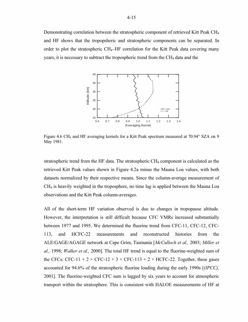
4-15

Demonstrating correlation between the stratospheric component of retrieved Kitt Peak CH4

and HF shows that the tropopsheric and stratospheric components can be separated. In

order to plot the stratospheric CH4–HF correlation for the Kitt Peak data covering many

years, it is necessary to subtract the tropospheric trend from the CH4 data and the

40

35

30

25

20

15

Altit

ude

(km

)

1.41.31.21.11.00.90.80.70.6Averaging Kernel

CH4 HF

Figure 4.6 CH4 and HF averaging kernels for a Kitt Peak spectrum measured at 70.94° SZA on 9 May 1981.

stratospheric trend from the HF data. The stratospheric CH4 component is calculated as the

retrieved Kitt Peak values shown in Figure 4.2a minus the Mauna Loa values, with both

datasets normalized by their respective means. Since the column-average measurement of

CH4 is heavily weighted in the troposphere, no time lag is applied between the Mauna Loa

observations and the Kitt Peak column-averages.

All of the short-term HF variation observed is due to changes in tropopause altitude.

However, the interpretation is still difficult because CFC VMRs increased substantially

between 1977 and 1995. We determined the fluorine trend from CFC-11, CFC-12, CFC-

113, and HCFC-22 measurements and reconstructed histories from the

ALE/GAGE/AGAGE network at Cape Grim, Tasmania [McCulloch et al., 2003; Miller et

al., 1998; Walker et al., 2000]. The total HF trend is equal to the fluorine-weighted sum of

the CFCs: CFC-11 + 2 × CFC-12 + 3 × CFC-113 + 2 × HCFC-22. Together, these gases

accounted for 94.6% of the stratospheric fluorine loading during the early 1990s [(IPCC),

2001]. The fluorine-weighted CFC sum is lagged by six years to account for atmospheric

transport within the stratosphere. This is consistent with HALOE measurements of HF at

4-16

54 - 56 km [Considine et al., 1999]. The time lagged fluorine-weighted CFC sum is shown

in Figure 4b. The HF variation due strictly to stratospheric change was determined from

(HF scaled by mean - lagged CFC sum scaled by mean) / (CFC scaled by mean).

The resulting plot of stratospheric CH4 vs. HF for the Kitt Peak dataset is shown in Figure

4.5c. The -7.8 × 102 slope of this dataset is consistent with the HALOE and MkIV slopes.

The coefficient of determinant, r2, is 0.19. Although the Kitt Peak correlation alone is

insufficient to justify a CH4–HF slope correction, its agreement with the HALOE and

MkIV data provides support for using Equation 4.4 to calculate tropospheric CH4 VMRs.

MkIV and HALOE data are only available for 1991 - present. Changing CFC VMRs in the

past will cause the CH4–HF slope to vary. We have extrapolated the CH4–HF slope, b(t),

from 1991 to 1977 by b(t) = b(1992) / fluorine-weighted CFC sum(t - 6 years), with the

fluorine-weighted CFC sum normalized to 1 in 1992.

4.11 References



Blake, D. R., and F. S. Rowland (1986), Worldwide increase in tropospheric methane,

1978-1983, J. Atmos. Chem., 4, 43-62.

Brown, L. R., J. S. Margolis, J. P. Champion, J. C. Hilico, J. M. Jouvard, M. Loete, C.

Chackerian, G. Tarrago, and D. C. Benner (1992), Methane and its isotopes - Current

status and prospects for improvement, J. Quant. Spectrosc. Radiat. Transfer, 48, 617-

628.

Considine, G. D., L. E. Deaver, E. E. Remsberg, and J. M. Russell (1999), Analysis of

near-global trends and variability in Halogen Occultation Experiment HF and HCl data

in the middle atmosphere, J. Geophys. Res., 104, 24297-24308.

Cunnold, D. M., L. P. Steele, P. J. Fraser, P. G. Simmonds, R. G. Prinn, R. F. Weiss, L. W.

Porter, S. O'Doherty, R. L. Langenfelds, P. B. Krummel, H. J. Wang, L. Emmons, X.

X. Tie, and E. J. Dlugokencky (2002), In situ measurements of atmospheric methane at

GAGE/AGAGE sites during 1985-2000 and resulting source inferences, J. Geophys.

Res., 107, doi:10.1029/2001JD001226.

4-17

Dlugokencky, E. J., K. A. Masarie, P. M. Lang, and P. P. Tans (1998), Continuing decline

in the growth rate of the atmospheric methane burden, Nature, 393, 447-450.

Dlugokencky, E. J., K. A. Masarie, P. P. Tans, T. J. Conway, and X. Xiong (1997), Is the

amplitude of the methane seasonal cycle changing?, Atmos. Environ., 31, 21-26.




edited.

Khalil, M. A. K., and R. A. Rasmussen (1983), Sources, sinks, and seasonal cycles of

atmospheric methane, J. Geophys. Res., 88, 5131-5144.

Luo, M., R. J. Cicerone, and J. M. Russell (1995), Analysis of Halogen Occultation

Experiment HF Versus CH4 correlation plots - Chemistry and transport implications, J.

Geophys. Res., 100, 13927-13937.

Margolis, J. S. (1988), Measured line positions and strengths of methane between 5500 and

6180 cm-1, Appl. Opt., 27, 4038-4051.

Margolis, J. S. (1990), Empirical values of the ground-state energies for methane

transitions between 5500 and 6150 cm-1, Appl. Opt., 29, 2295-2302.

McCulloch, A., P. M. Midgley, and P. Ashford (2003), Releases of refrigerant gases (CFC-

12, HCFC-22 and HFC-134a) to the atmosphere, Atmos. Environ., 37, 889-902.

Miller, B. R., J. Huang, R. F. Weiss, R. G. Prinn, and P. J. Fraser (1998), Atmospheric

trend and lifetime of chlorodifluoromethane (HCFC-22) and the global tropospheric

OH concentration, J. Geophys. Res., 103, 13237-13248.

Park, J. H., J. M. Russell, L. L. Gordley, S. R. Drayson, D. C. Benner, J. M. McInerney, M.

R. Gunson, G. C. Toon, B. Sen, J. F. Blavier, C. R. Webster, E. C. Zipf, P. Erdman, U.

Schmidt, and C. Schiller (1996), Validation of Halogen Occultation Experiment CH4

measurements from the UARS, J. Geophys. Res., 101, 10183-10203.

Pine, A. S. (1992), Self-Broadening, N2-broadening, O2-broadening, H2-broadening, Ar-

broadening, and He-broadening in the ν3 band Q-branch of CH4, J. Chem. Phys., 97,

773-785.

Pine, A. S. (1997), N2 and Ar broadening and line mixing in the P and R branches of the ν 3

band of CH4, J. Quant. Spectrosc. Radiat. Transfer, 57, 157-176.

4-18

Russell, J. M., L. E. Deaver, M. Z. Luo, R. J. Cicerone, J. H. Park, L. L. Gordley, G. C.

Toon, M. R. Gunson, W. A. Traub, D. G. Johnson, K. W. Jucks, R. Zander, and I. G.

Nolt (1996), Validation of hydrogen fluoride measurements made by the Halogen

Occultation Experiment from the UARS platform, J. Geophys. Res., 101, 10163-10174.

Russell, J. M., L. L. Gordley, J. H. Park, S. R. Drayson, W. D. Hesketh, R. J. Cicerone, A.

F. Tuck, J. E. Frederick, J. E. Harries, and P. J. Crutzen (1993), The Halogen

Occultation Experiment, J. Geophys. Res., 98, 10777-10797.

Sen, B., G. C. Toon, J. F. Blavier, E. L. Fleming, and C. H. Jackman (1996), Balloon-borne

observations of midlatitude fluorine abundance, J. Geophys. Res., 101, 9045-9054.

Toon, G. C. (1991), The Jet Propulsion Laboratory MkIV Interferometer, Opt. Photonics

News, 2, 19-21.

Walker, S. J., R. F. Weiss, and P. K. Salameh (2000), Reconstructed histories of the annual

mean atmospheric mole fractions for the halocarbons CFC-11, CFC-12, CFC-113, and

carbon tetrachloride, J. Geophys. Res., 105, 14285-14296.

Wallace, L., and W. Livingston (1990), Spectroscopic observations of atmospheric trace

gases over Kitt Peak: 1. Carbon dioxide and methane from 1979 to 1985, J. Geophys.

Res., 95, 9823-9827.



doi:10.1029/2001GL014537.

A-1

Appendix A

TECHNICAL DOCUMENTATION FOR THE CALTECH COLUMN

OBSERVATORY

A.1 Summary

Three FTS observatories were assembled at Caltech during 2003 – 2006. These are currently deployed in Park Falls, Wisconsin (IFS1); Darwin, Australia (IFS2); and Pasadena, California (IFS3). Each observatory consists of a standard 20’ x 8’ x 8.5’ steel shipping container, which has been modified by Martin Container according to our specifications to include reinforcement of the roof with 2.5” square steel tubing, addition of a 12” hole for the solar input beam, electrical wiring and breakout box, telephone wiring, heater/air conditioner, and welded nuts for mounting the Bruker IFS125. A Bruker IFS125 spectrometer is installed in each container. The IFS125 feet are connected to 0.75” thick aluminum beams, which are then bolted onto I-beams. The I-beams are bolted to nuts which are welded to the container frame. A fiberglass telescope dome is mounted on the reinforced section of the container roof. Inside the dome, a Bruker solar tracker is installed on an 8” diameter aluminum cylinder with 1” walls. This construction is intended to minimize any vibrations or misalignment. A network camera and weatherstation are also mounted on the roof. The complete observatory consists of the IFS125 spectrometer, scroll pump, solar tracker, telescope dome, weatherstation, NTP-GPS satellite receiver, network camera, heaters (for IFS125, solar tracker, and scroll pump), temperature sensors, current and voltage sensors, and power systems. Each of these systems is monitored and/or controlled with a Diamond Systems Hercules board and an additional control board. The Hercules board includes four serial ports, used for communication with the solar tracker, telescope dome, weatherstation, and modem. The Hercules board includes 32 wide-range analog inputs for monitoring temperatures, voltage, currents, and pressure of the scroll pump. Five digital I/O lines of the Hercules board are used to command power to the solar tracker, telescope dome, modem, IFS125, and IFS125 reset line. The IFS125, network camera, NTP-GPS satellite time receiver, and uninterruptible power supply are commanded within the local area network. Many of the observatory devices are commercial and have useful manuals. The original manual is the best starting point for troubleshooting a specific piece of the equipment, and I have not attempted to duplicate any of that information here. This appendix is meant to fill the remaining information gaps. For example, Bruker has provided no documentation for the IFS125. Similarly, the data acquisition software is entirely custom-written and does not have formal documentation.

A-2

A.2 Instrumentation

A.2.1 Bruker IFS125 Spectrometer

Model: Bruker Optics – IFS125 Bruker Optik GmbH Rudolf-Plank-Str. 27 D-76275 Ettlingen Germany www.brukeroptics.com Tel: (07243) 504 600 Fax:(07243) 504 698 Email: [email protected]

Description:

The Bruker IFS125 Michelson interferometer with electronics based on the Brault method. J.W. Brault (1996). New approaches to high-precision Fourier transform spectrometer design. Applied Optics, Vol. 35; No. 16; 2891 – 2896. No manual exists for the IFS125. Connection to Hercules Computer:

Network 192.168.1.101 Power is controlled by an optical fiber which is driven digitally. Reset is controlled by an optical fiber which is driven digitally. Direct Communication:

Use web browser to connect to 192.168.1.101 OPUS Registration Details

Name = “IFS 125HR” Company = “CALIFORNIA INSTITUTE OF TECHNOLOGY” Instrument = “BI020002” OPUS Serial2 = “576168593” Key2 = “4244244Z440Z” IFS125 Serial Numbers

IFS1 (Park Falls) – SN02 IFS2 (Darwin) – SN13 IFS3 (Pasadena / Lamont) – SN20 A.2.1.1 Laser (Spectra-Physics 117A)

The laser signal is measured by two photodiode detectors, which Bruker refers to as Laser Detector A and Laser Detector B. These detectors are connected to the laser detector board in the interferometer compartment. The laser signal can be observed directly with an oscilloscope connected to LAS-A, LAS-B, and GND on the laser detector board.

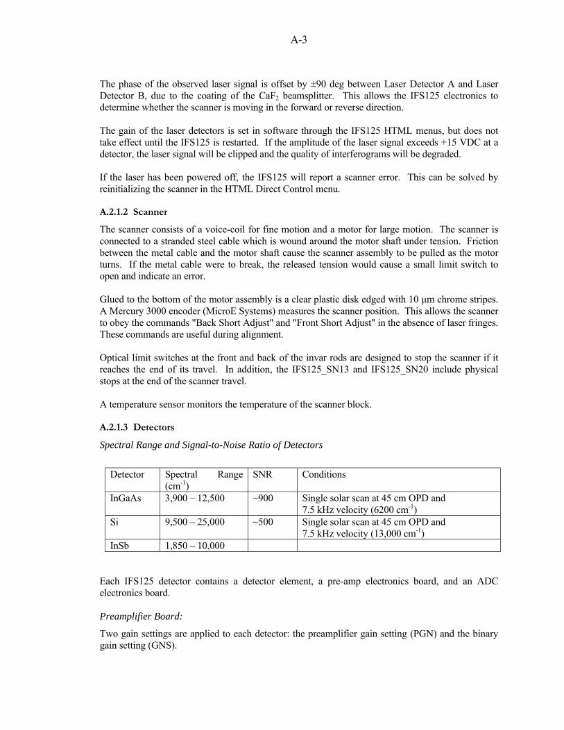
A-3

The phase of the observed laser signal is offset by ±90 deg between Laser Detector A and Laser Detector B, due to the coating of the CaF2 beamsplitter. This allows the IFS125 electronics to determine whether the scanner is moving in the forward or reverse direction. The gain of the laser detectors is set in software through the IFS125 HTML menus, but does not take effect until the IFS125 is restarted. If the amplitude of the laser signal exceeds +15 VDC at a detector, the laser signal will be clipped and the quality of interferograms will be degraded. If the laser has been powered off, the IFS125 will report a scanner error. This can be solved by reinitializing the scanner in the HTML Direct Control menu. A.2.1.2 Scanner

The scanner consists of a voice-coil for fine motion and a motor for large motion. The scanner is connected to a stranded steel cable which is wound around the motor shaft under tension. Friction between the metal cable and the motor shaft cause the scanner assembly to be pulled as the motor turns. If the metal cable were to break, the released tension would cause a small limit switch to open and indicate an error. Glued to the bottom of the motor assembly is a clear plastic disk edged with 10 μm chrome stripes. A Mercury 3000 encoder (MicroE Systems) measures the scanner position. This allows the scanner to obey the commands "Back Short Adjust" and "Front Short Adjust" in the absence of laser fringes. These commands are useful during alignment. Optical limit switches at the front and back of the invar rods are designed to stop the scanner if it reaches the end of its travel. In addition, the IFS125_SN13 and IFS125_SN20 include physical stops at the end of the scanner travel. A temperature sensor monitors the temperature of the scanner block. A.2.1.3 Detectors

Spectral Range and Signal-to-Noise Ratio of Detectors

Detector Spectral Range

(cm-1) SNR Conditions

InGaAs 3,900 – 12,500 ~900 Single solar scan at 45 cm OPD and 7.5 kHz velocity (6200 cm-1)

Si 9,500 – 25,000 ~500 Single solar scan at 45 cm OPD and 7.5 kHz velocity (13,000 cm-1)

InSb 1,850 – 10,000 Each IFS125 detector contains a detector element, a pre-amp electronics board, and an ADC electronics board. Preamplifier Board:

Two gain settings are applied to each detector: the preamplifier gain setting (PGN) and the binary gain setting (GNS).

A-4

The binary gain may be set for both the master and slave detectors, using the GNS and SG2 commands. The binary gain settings are fixed. These choices are: 1, 2, 4, 8, and 16. The preamp gain choices can be adjusted by changing resistors on the pre-amp electronics board. These resistors are labeled Ra, Rb, Rc, and Rd. In software, these choices appear as Ra = 0, Rb = 1, Rc = 2, and Ref = 3. Bruker has provided us with the preamp schematics. For the IFS125 detectors, these values are currently:

InGaAs Si InSb Ra 3090 ohms 7680 ohms 1500 ohms Rb 3650 ohms 9090 ohms 3600 ohms Rc 750,000 ohms 1,500,000 ohms 25,000 ohms Rd (ref) 2700 ohms 20,000 ohms 10,000 ohms

ADC Board:

This is a 24-bit, two-channel ADC with a maximum sampling frequency of 96 kHz. When taking two points per laser fringe (as required for wideband NIR work in dual-acquistion mode), this limits the maximum theoretical scanner velocity to 40 kHz. However, the Bruker data acquisition has struggled with other problems and has never achieved this 40 kHz potential. To set the preamp gain, it is necessary to explicitly select the detector. For this reason, it is not possible to set the preamp gain of the slave detector. Bruker has implemented the DC channels in a peculiar way. One channel of the ADC is assigned to DC output and one channel is assigned to AC output. Dual-acqusition in DC mode records the InGaAs DC channel together with the Si DC channel as observed through the other (AC) InGaAs channel. Dual-acquisition in AC mode records the Si AC channel together with the InGaAs AC channel as observed through the other (DC) Si channel. It necessary to explicitly select a detector in order to set its preamp gain. This strange dual-acquisition signal-forwarding makes it difficult to deteremine what gain is being changed. Here is a guide.

Detector Description Address Action RT-Si Diode DC [Int Pos 1] 0x4020 Sets InGaAs gain RT-InGaAs DC [Int Pos 1 0x4021 Sets InGaAs gain RT-Si Diode DC + InGaAs DC [Int Pos 1] 0x4022 Sets InGaAs gain RT-Si Diode AC [Int Pos 2] 0x4040 Sets Si gain RT-InGaAs AC [Int Pos 2] 0x4041 Sets Si gain RT-Si Diode AC + RT-InGaAs AC [Int Pos 2] 0x4042 Sets Si gain LN-InSb FOV=30 [Int Pos 4] 0x40C0 Sets InSb gain

A.2.1.4 Tungsten Lamp

A +12 VDC power supply for the tungsten lamp is located in the front panel electronics unit. A potentiometer labeled Vadj allows the voltage of the power supply to be adjusted with a flathead screwdriver, which changes the temperature of the tungsten lamp. We have not adjusted this. The typical operating temperature for a tungsten filament is 3000 K.

A-5

A temperature sensor monitors the temperature of the metal block that contains the tungsten lamp. If the measured temperature exceeds 60 deg C, the tungsten lamp will be shut off. Normally, a water circulation unit is connected externally to cool the source block. We have disconnected the water circulation units. Time required for lamp stabilization

The drift of the lamp during the first ten minutes of operation appears to have little to do with the water circulation unit. The lamp needs 2-3 minutes to stabilize, regardless of whether the cooler is connected or not. The cooler does not appear to improve the lamp performance during minutes 3 - 10 of operation. Measurements of ZPD amplitude at one minute intervals (21 Jan 2004): ZPD InGaAs at each minute without cooler: 0.413, 0.408, 0.406, 0.405, 0.405, 0.405, 0.405, 0.405, 0.406, 0.405, 0.405 ZPD InGaAs at each minute with cooler: 0.420, 0.412, 0.409, 0.410, 0.404, 0.398, 0.399, 0.394, 0.392, 0.396, 0.398 ZPD Si at each minute without cooler: 0.320, 0.307, 0.305, 0.304, 0.304, 0.304, 0.303, 0.303, 0.303, 0.303, 0.302 ZPD Si at each minute with cooler: 0.341, 0.329, 0.323, 0.321, 0.320, 0.320, 0.321, 0.319, 0.318, 0.321, 0.321 A.2.1.5 Valves and Vacuum System

The IFS125 includes four normally-closed valves. These allow separate evacuation and venting of the interferometer and sample compartment. After removing the sample compartment, we have capped the connections for evacuating and venting the sample compartment. The valve for evacuating the IFS125 is a Leybold Vacuum Right Angle Valve. The valve has two terminal blocks, for power (orange) and for commanding the valve (green). We have connected the power input directly to the AC container power (220 VAC in Park Falls; 230 VAC in Darwin). In the case of power outage, the normally-closed valve will shut. The command line connects to the IFS125 and consists of two wires. The brown wire is connected to pin “a” of the terminal block; white wire is connected to pin “d” of the terminal block. In addition, a set of resistors connect pins “a” and “d”. The valve is commanded directly through the IFS125 control software provided by Bruker (VAC=0; VAC=1). The Leybold Vacuum Right Angle Valve failed in Darwin, after a lightning strike. We replaced it with a new valve. The damaged valve was repaired and installed in ifs125_3. After the repair, we were missing the necessary German parts for the fuse holder. The fuse and fuse holder are now soldered to the line voltage outside of the valve. The IFS125 includes a Leybold Vakuum Thermovac Transmitter for measuring the pressure of the interferometer compartment. There is a differential pressure gauge for measuring the relative pressure between the interferometer compartment and the sample compartment. The differential pressure gauge is located in the Electronics Panel. This gauge is unnecessary for us and we have disconnected its tubing.

A-6

A.2.1.6 Small Devices with Control Area Network Boards

Each small motor in the IFS125 is commanded by a Control Area Network (CAN) board. These include: the source selection mirror (source compartment), the tungsten flip mirror (source compartment), the field stop wheels (source and interferometer compartments), and the moving detector mirror (detector compartment). Each CAN board has four connectors: CAN1, CAN2, MOT0, and MOT1, allowing it to control two motors. The addressing of the CAN boards is indicated by jumpers labeled either "JAD" or "JPADR". There are five grounding jumpers labeled 2, 4, 8, 16, 32. The setting of their jumpers matches the "Mot Number" in the pdf list of CAN devices. The source holder and vacuum control seem to have a different type of CAN board. The list of CAN devices can be found in the IFS125 “Full Report”. A.2.1.7 Electronics Systems

The front panel contains of the electronics box many connectors and blinkenlights. Main Power Input – Upper Right Panel

Main input power connection with switch and indicator light – The main input power for the IFS125 is connected to the Uninterruptible Power Supply. Power connection to the IFS125 electronics unit – A short power cable connects the main input power to the electronics unit. Connection for sources – A D-sub connector supplies power and control to the tungsten lamp. Connection for valves – Supplies power and control to the valves. RJ45 connection for Leybold Vakuum Thermovac Transmitter Connection for laser input – Connects to the laser power supply. Power Supply for the Electronics Unit

The Power Supply Block for the Electronics Unit is powered by a short power cable from the Main Power Input Panel. Three LEDs indicate that the Electronics Unit has +5 VDC, +12 VDC, and -12 VDC power. These LEDs are normally on. The round CAN-bus connector is unused. Electronics Unit

The electronics unit consists of three boards: EWS15 – Embedded Web Server Electronics Board Connection for "COM1" – An unused 9-pin D-sub connector. It is intended for commercial RS232 devices. Connection for "LPT1" – An unused 25-pin D-sub connector. This connector contains various analog signal used for trouble-shooting. Because it might be useful, Bruker won't tell us what it does. RJ45 connector for network – 10BASE-T ethernet communication to IFS125. Status LEDs:

RES – Resets the IFS125 electronics. Equivalent to switching off and on the power switch. TX – Ethernet transmission. Indicates that the IFS125 is actively communicating. RX – Ethernet reception. ST – Unknown SG – Unknown

A-7

SCT– Scanner Electronics Board

Interferometer LEDs: ERR – Error (usually due to missing laser signal or problem with scanner) FWD – Scanner direction forward TKD – Acquiring data. In later versions of the firmware, the TKD light does not correctly indicate that data is being acquired.

ANA.25 – Analog Electronics Board

Connection to Scanner Motor “OMOT” – This cable connects to a flange under the scanner compartment. The cable enables power/communication both to the scanner motor and the MicroE Systems Mercury 3000 encoder. Control Area Network, Icon, and Detector Signal Block

These connectors are located in the final block. A 9-pin D-sub connector has been added to replace the sample compartment flaps.

A-8

A.2.1.8 HTML Software Interface

The IFS125 is commanded using an HTML interface. Connect a web browser to 192.168.1.101 for the IFS125 Direct Control Menus. This is the most direct communication with the IFS125. Both OPUS and the QNX data acquisition software send all commands via the HTML interface. Measurement Menus Measurement Status Direct Command Entry Messages Diagnostics Status of Scanner, Detectors, HeNe Laser, IR Source, Automation Units, and Instrument Ready Service View Instrument Configuration Full Report Log Buffer (buffer since IFS125 was turned on) Beep (beeps if IFS125 is communicating) List of commands (command names, their descriptions, and current values) Check Detectors (similar menu options for other components) Reset Instrument (one of three ways to reset the IFS125) Last CAN answer Edit hardware configuration EWS TCPIP Setup Menu (IP address assignment) Set Time & Date Service links Direct Control Panel Current temperature and pressure Vacuum Control Commands Scanner Control Commands

A-9

A.2.1.9 IFS125 Direct Commands and Allowed Values

All commanding of the IFS125 occurs through the IFS125 HTML interface, using a series of direct commands. These consist of three letter acronyms which are defined by Bruker. The OPUS data acquisition software and Hercules data acquisition software are user-friendly overlays for this communication. At their heart, these programs simply send direct commands to the IFS125 through the HTML interface. The IFS125 direct commands and accepted values are compiled below. Although some of the commands are completely useless, they are included here for completeness. Useful Direct Commands for IFS125

Command Description Accepted Values ADM Adjust modes 0=Reinit Scanner; 1=Fast Adjust Mode (40 kHz);

2=Stop Mode; 3=Slow Adjust Mode (5 kHz); 4=Front Short Adjust Mode (voice coil); 5=Back Short Adjust Mode (voice coil)

AMD Acquisition mode 3=sliced data AQM Acquisition mode DD=Double sided, forward-backward; SD=Single

sided, forward-backward; DN=Double sided; SN=Single sided

AP2 Exit field stop 500=0.5 mm; 800=0.8 mm; 1000=1 mm; 1150=1.15 mm; 1300=1.3 mm; 1500=1.5 mm; 1700=1.7 mm; 2000=2 mm; 2500=2.5 mm; 3150=3.15 mm; 4000=4 mm; 5000=5 mm; 6300=6.3 mm; 8000=8 mm; 10000=10 mm; 12500=12.5 mm

APT Input field stop 500=0.5 mm; 800=0.8 mm; 1000=1 mm; 1150=1.15 mm; 1300=1.3 mm; 1500=1.5 mm; 1700=1.7 mm; 2000=2 mm; 2500=2.5 mm; 3150=3.15 mm; 4000=4 mm; 5000=5 mm; 6300=6.3 mm; 8000=8 mm; 10000=10 mm; 12500=12.5 mm

BRK Break 1=Abort; 2=Stop; 4=Skip waiting for delay; 8=Skip waiting for trigger; 16=Skip waiting for ready; 32=Stop

DTC Detector setting (varies with instrument)

For ParkFalls_ifs1:16416=RT-InGaAs [Internal Pos.1]; 16417=RT -InGaAs (DC) [Internal Pos.1]; 16448=RT-Si Diode [Internal Pos.2]; 16449=slave [Internal Pos.2]; 16450=Si- Diode & Slave [Internal Pos.2]

GNS Signal gain 1=x1; 2=x2; 4=x4; 8=x8; 16=x16 HFW Wanted high frequency limit [double] HPF High pass filter 0=Open; 1=On LFW Wanted low frequency limit [double] LPF Low pass filter 5.00=5 kHz; 10.0=10 kHz; 20.0=20 kHz; 40.0=40

kHz; 40.0=Open LSR Laser on/off 0=Off; 1=On LWN Laser wavenumber [double] NSS Number of scans [int] PGN Preamplifier gain 0=A; 1=B; 2=C; 3=Ref PHR Phase resolution [double]

A-10

RES Resolution [double] SRC Source 0=Off All; -104=NIR Off; 104=NIR;

201=Emission back parallel input VAC Vaccum control 0=Standby; 1=Evacuate; 2=Vent SG2 Left channel signal gain 1=x1; 2=x2; 4=x4; 8=x8; 16=x16 VEL Velocity 5.00=5 kHz; 7.50=7.5 kHz; 10.0=10 kHz; 15.0=15

kHz; 20.0=20 kHz; 30.0=30 kHz; 40.0=40 kHz; 60.0=60 kHz; 80.0=80 kHz

Unused Direct Commands for IFS125:

Command Description Accepted Values CHN Measurement channel FLP Flaps control Flaps not installed IM0 Interferometer motor 0 IM1 Interferometer motor1 OF1 Optical filter at det. pos. 1 and 2 Optical filter not installed OF2 Optical filter at det. pos. 3 and 4 Optical filter not installed CPJ I-factor outer motor control CPQ P-factor outer motor control CPS I-factor inner motor control CPT P-factor inner motor control PLL PLLdummy AAR Automatic Accessory

Recognition

ABP Absolute peak location BMS Beamsplitter CHK Check CMA Correlation mask CNM Operator name COR Correlation CPF Compensation filter CPI Control parameter I CPP Control parameter P DDM Display during measurement DEL Delay before measurement DLR Delay between repeats DLY Stabilization delay FMD Filter mode FSS Full scale scan ITS Instrument test class ITI Instrument test interval JMW Test parameter LFT Lifetime MAC Macro MIN Measurement time in minutes RDX Ready mask RDY Instrument ready status

A-11

REP Repeat the measurement SFM Sample form SNM Sample name SON External trigger SOT Scans or minutes TDL FT to do list TRW IR/TRW selection TSR Tolerance scan range UWN Channel specific LWN VLV Valve control XND XA delay in nsec XXA DSP testcommand _EP Send EWS parameter to DSP _GI Get information _GP Get intermediate result _GR Get result _ME Measure _MX Multiplexer IR/TRW _PS Periodic status request _SP Set parameter _TR Trigger measurement

A-12

A.2.1.10 Alignment Procedure

It is necessary to realign the IFS125 after moving the observatory. The notes below provide a step-by-step procedure, based on the method of Jean-Francois Blavier.

Initial Alignment and Preparations

Re-assemble scanner, beamsplitter, and dichroic Release locking screws of IFS125 base plates Release locking screws of mirrors After verifying that the interferometer is misaligned: Check that the interferometer base plate is level with respect to top of the compartment. Adjust scanner rods to be level, meaning equidistant from vacuum support bars. Laser Alignment

Criteria: - Laser beam position on round baseplate window. - Laser beam position on upper prism. - Laser beam position on cube corner - Laser beam position on beamsplitter; must travel through notch in coating - Laser modulation at detectors A and B The first two criteria are controlled by adjusting the alignment of the lower prism. It may be necessary to compromise the adjustment between these two. The next two criteria are controlled by adjusting the alignment of the upper prism. The last criteria is controlled by alignment of interferometer.

Before making any adjustment: - Laser must warm up for twenty minutes, regardless of laser beam appearance. - Using a piece of paper, look at laser image on detectors A and B at different scanner positions.

Adjust position of laser within rectangular tube.

- Adjustment of laser was not necessary previously and is unlikely. Do this only if the lower prism can not be adjusted to bring it onto the round window and upper prism OR if the laser beam is not on the lower prism. - If laser is misaligned, this can be compensated by adjusting the lower prism.

Adjustment of incoming laser beam at lower prism

- This positions the laser beam on the round interferometer baseplate window and face of upper prism. - Laser spot should be aligned on round window of interferometer base plate and face center of upper prism. Use mirror to see upper prism.

Turn on IFS125 power.

- Connect oscilloscope to Gnd, Laser A, and Laser B on laser detector electronics board (second ground not necessary).

Adjustment of laser beam at upper prism

- This is the most likely to be misaligned - Use Back Short Adjust Mode

A-13

- Cover detectors A and B with paper, so modulation is easily visible - Adjust three alignment screws of upper prism so laser spots overlap and modulate at detectors A and B - Proper modulation will appear as a round coincident spot, that blinks light and dark - At Back Short Adjust, laser beam should fall within the cube corner and within notch of beamsplitter

Check that laser beam is positioned properly at detectors A and B

- Use Back Short Adjust Mode - Check that laser beam is not clipped by notch in detector - Adjust three sets of screws for detectors A and B to position laser beam at detectors - Lock washers under the four mounting screws of detectors A and B can be used as tip-tilt adjustment - Possible to translate beam by adjusting prisms in Back Short Adjust Mode: - If a vertical translation is necessary:

- Translate upper prism down = beam into cube corner = beam up on parabolic laser mirror - If a horizontal translation is necessary (beam on edge of detector notch, but detectors have no more play):

- Translate upper and lower prisms together to move sideways on parabolic laser mirror - When scanning, detectors A and B should peak together. Otherwise, this suggests that the beam is on the edge of an optic. It is likely to be the laser detector edge, because this is the smallest optic. - To move the laser image sideways on the laser detector, if it necessary to tip/tilt the assembly in either the horizontal or vertical planes. It is easy to inadvertently tip/tilt the assembly in the horizontal plane while adjusting it.

Return to Front Short Adjust Mode and check laser beam overlap at detector A.

- If beams do not overlap and laser amplitude decreases toward ZPD, then there is a problem in the alignment of the fixed cube corner.* At ZPD, no adjustment of the prisms can not compensate for this error. - Look for modulation on detectors as the scanner is still - Check that beam is circular, with good overlap, and blinks light/dark. - This shows that the laser is correctly aligned on the axes of the interferometer, assuming that the two axes of the interferometer are parallel.

*Necessary to adjust the fixed cube corner if any of the following are true:

- Lower amplitude at detectors A and B at ZPD than at Back Short Adjust - Laser beam overlaps at Back Short Adjust, but not at ZPD - Poor modulation of Si detector

The purpose of the upper prism is to align the laser beam parallel to the interferometer axis. This can be falsely accomplished at all positions of the moving cube corner, except ZPD. If there is misalignment of the interferometer, then each position will require a different adjustment of the moving cube corner. If the interferometer is correctly aligned, then the adjustment of the upper prism will be optimum for all positions of the moving cube corner. This should not typically be necessary. If the fixed cube needs to be aligned:

- Release four locking screws on back of fixed cube corner - Fine-threaded top and side adjustment screws determine alignment of fixed cube corner.

A-14

- Visually align laser beam to be coincident at detector A. If the amount of displacement is independent of path difference, then this adjustment can be done at any position of the moving cube corner. - Look for circular spot, with good overlap, that blinks light/dark when scanner is still. - Use oscilloscope to refine adjustment of fixed cube corner while watching amplitude of detector A in scanner Front Short Adjust Mode. - Check amplitude of detector A in scanner Back Short Adjust Mode. - When finished, tighten four locking screws of fixed cube corner while monitoring that this does not affect amplitude of detector A

Final result

- Expecting total amplitude to be ~15 V at detectors A and B with much less than 15% variability front-to-back. - Total amplitude depends on laser detector gain and may be different between spectrometers.

Tungsten Beam Alignment

Criteria: - Even illumination of entrance and exit optics - Alignment of lamp beam on entrance and exit field stop wheels - Detector signal peaked by adjusting detector focal optics - Line depth maximized and line width minimized by adjusting interferometer entrance and exit mirrors It is necessary to align the flat entrance and exit mirrors because the incoming beam may not be parallel to the interferometer axis. There are three steps to align the flat entrance and exit mirrors to center the field stop on the interferometer axis: - Visual alignment of lamp image on exit field stop - Visual alignment of laser image on entrance and exit field stops - Fine, iterative alignment by recording lamp spectra and fitting HCl lines to determine width/ILS While measuring modulation efficiency at DC testpoints on Si and InGaAs detectors, where modulation = ZPD peak value / ZPD average value:

Adjust entrance optics in source compartment - With tungsten lamp on, adjust spherical mirror in source compartment to center filament image on field stop wheel.

Trace beam path and verify that optics are properly illuminated.

- Adjust exit optics in interferometer and detector compartments - Look for obvious illumination errors, which suggest misalignment during transport - If necessary, adjust off-axis parabolic mirror at exit of interferometer to center IR beam on flat exit mirror. - Always adjust flat exit mirror to center IR beam on exit field stop. - Finally adjust off-axis parabolic mirror in detector compartment (first mirror). If this mirror is not well illuminated, repeat the previous two steps. Note that clipping the exit field stop image will decrease the linewidth because the effective field stop is smaller, but will introduce an ILS error.

Align off-axis parabolic detector mirrors

A-15

- Using OPUS or DC testpoints, adjust focal mirrors in detector compartment to peak detector signal

Return laser beam to source compartment with Tungsten lamp off

- Detectors A and B can be moved vertically. Pull the side tab to release the translation stage. This allows laser beam to return toward the source compartment for alignment purposes. - Choose 0.5 mm field stop - Lower detector A. Align flat interferometer exit mirror to center laser on exit field stop. Replace detector A. - Lower detector B. Align flat interferometer entrance mirror to center laser on entrance field stop. Replace detector B. - Turn on Tungsten lamp. If lamp beam is imaged from entrance field stop onto exit field stop, then the alignment has worked well.

Ideally, this technique would achieve the final alignment. However: - The laser is too small for the 0.5 mm field stop. - Need proper alignment in the near-IR, not at 15798 cm-1. - The prism and beamsplitter coating affect the laser beam and near-IR beam differently.

Iterative adjustment of flat entrance and exit mirrors to center field stop on interferometer axis using HCl lines.

- First record spectrum with no changes to alignment. - Then iteratively adjust entrance and exit mirrors around this alignment, recording a spectrum at each position. Total will be five (original plus four adjustments). - Top diagonal = horizontal adjustment; bottom diagonal = vertical adjustment - The error which is corrected is less than ~1/4 diameter of solar image

I. Record two spectra with no changes to alignment IIa. Adjust both top screws of flat exit mirror to fixed maximum value – This is DC value A (e.g. -1.954 V)

Adjust flat entrance mirror top diagonal CW to a lower fixed value – This is DC value B (e.g. -1.800 V) Adjust flat exit mirror top diagonal – Return to DC value A (e.g. -1.954 V). Record spectrum.

IIb. Adjust flat entrance mirror top diagonal CCW – Return to DC value B.

Adjust flat exit mirror top diagonal – Return to DC value A. This returns to alignment in I. IIIa. Adjust flat entrance mirror top diagonal CCW – Return to DC value B.

Adjust flat exit mirror top diagonal – Return to DC value A. Record spectrum.

IIIb. Adjust flat entrance mirror top diagonal CW – Return to DC value B.

Adjust flat exit mirror top diagonal – Return to DC value A. IVa.Adjust flat entrance mirror bottom diagonal CW – Return to DC value B.

Adjust flat exit mirror bottom diagonal – Return to DC value A. Record spectrum.

IVb. Adjust flat entrance mirror bottom diagonal CCW – Return to DC value B.

Adjust flat exit mirror bottom diagonal – Return to DC value A.

A-16

Va. Adjust flat entrance mirror bottom diagonal CCW – Return to DC value B.

Adjust flat exit mirror bottom diagonal – Return to DC value A. Record spectrum.

- Use OPUS to fit average WHM for region of HCl lines. Previously used 5730 – 5780 cm-1 - Would be preferable to also use peak depth, but this is not available with OPUS. - From WHM, determine best alignment.

- This assumes that the alignment is symmetrical, not skewed. Re-iterate on steps I – V starting at the newly determined best position with smaller increments of adjustment. Align off-axis parabolic detector mirrors again - Using OPUS or DC testpoints, adjust focal mirrors to peak detector signal - Measure modulation efficiency again A.2.1.11 Previous Alignment Results

Using the DC testpoints on the IFS125 detectors, it is possible to directly observe the modulation efficiency at ZPD. Previous results are listed below. For caltech_ifs1: InGaAs ~ 80% and Si ~80%. For parkfalls_ifs1: InGaAs 84% and Si 77%. For caltech_ifs2: DC testpoints were not added until late in the spring, and the modulation efficiency was not measured. For darwin_ifs2: InGaAs 78% and Si 62%.

A-17

A.2.1.12 Acceptance Test Standards

The acceptance test is based on spectra of the 10 cm cell containing 5.0 hPa HCl gas. Typically, the cell is mounted in source compartment, but it can also be placed in the detector compartment. Acceptance criteria: Peak Amplitude of InGaAs and Si interferograms. Width and "relative intensity" of HCl lines in the 5730 - 5780 cm-1 region. Appearance of peak symmetry. Signal-to-noise ratio Results below were recorded in Park Falls, Wisconsin on 10 Aug 2004 using three different 10 cm HCl cells. Parameters: Dual-acquisition spectrum with four scans (forward-reverse). Resolution: 0.0125 cm-1. Zerofilling: 2. Gains: Reference (InGaAs 2700 ohm; Si 20,000 ohm). Scanner velocity: 10 kHz; high and low pass filters on. Aperture: 1.3 mm. Source: Tungsten lamp. Water circulation disconnected during the recording of these spectra. Air temperature: 20.0 deg C; Lamp temperature: 35 - 45 deg C. IFS125 Pressure: < 2 mb

A-18

Cell #1 pa30040810l0aax_Cell1.2 Si Peak Amp (For; Rev)

InGaAs Peak Amp (For; Rev)

Wave number

Abs. Intens.

Rel. Intens.

Width Thresh hold

S:N Ratio5745 - 5746cm-1

12740; 12559

6995; 6688

5735.1369 0.160 0.058 0.0150 43.274 986.45

5739.2901 0.084 0.134 0.0160 100.501 5749.8218 0.167 0.050 0.0150 37.425 5753.9924 0.096 0.120 0.0160 90.124 5763.2397 0.177 0.038 0.0150 28.831 5767.4248 0.118 0.097 0.0160 72.956 5779.5767 0.144 0.070 0.0150 52.340 Avg 0.0154 Cell #2 pa30040810l0aax_Cell2.2 12478; 12301

6713; 6484

5735.1369 0.157 0.057 0.0150 43.173 1032.6

5739.2901 0.081 0.132 0.0160 100.341 5749.8218 0.164 0.049 0.0150 37.343 5753.9924 0.094 0.118 0.0160 89.550 5763.2397 0.174 0.038 0.0140 28.883 5767.4248 0.116 0.096 0.0160 72.539 5779.5767 0.142 0.068 0.0150 51.849 Avg 0.0153 Cell #3 pa30040810l0aax_Cell3.4 12775; 12562

6851; 6701

5735.1369 0.160 0.060 0.0150 43.593 1001.65

5739.2901 0.081 0.138 0.0160 100.374 5749.8214 0.166 0.052 0.0150 37.885 5753.9924 0.093 0.124 0.0160 90.269 5763.2397 0.177 0.040 0.0150 28.866 5767.4248 0.115 0.101 0.0160 73.570 5779.5767 0.143 0.072 0.0150 52.395 Avg 0.0154

A-19

A.2.1.13 HCl Cells

Bill O'Rourke O'Rourke Enterprises 694 Main St. P.O. Box 52 Lumberton, NJ 08048 USA Tel: 609-265-0751 Fax: 609-265-1683 Email: None Description:

The first three HCl cells have 4.9 cm diameter Infrasil windows (Esco Products), fused into 10.0 cm x 5.0 cm diameter silica with a graded quartz-to-pyrex seal between the tube and a teflon valve. The cells were manufactured by Rick Gerhart and filled with 5.0 hPa HCl at JPL by Kevin Hickson on 15-April-2004. Infrasil HCl cells: Cell #1 – (Park Falls) Cell #2 – 5.02 hPa (Lauder) Cell #3 – 5.14 hPa (currently in Darwin; unused) The second three HCl cell have 4.0 cm diameter Sapphire windows (Esco Products) fused into 10.0 cm x 4.0 cm diameter tube with a graded quartz-to-pyrex seal between the tube and Teflon valve. The cells were manufactured by Bill O’Rourke and filled with 5.0 hPa HCl at JPL by Kevin Hickson. Sapphire HCl cells: Cell #4 – 5.0316 hPa (Caltech) Cell #5 – 5.0196 hPa (Darwin) Cell #6 – 5.1369 hPa (University of Bremen)

A-20

A.2.2 Bruker Solar Tracker

Bruker Optics – Solar Tracker Bruker Optik GmbH Rudolf-Plank-Str. 27 D-76275 Ettlingen Germany www.brukeroptics.com Tel: (07243) 504 600 Fax:(07243) 504 698 Email: [email protected] Description:

The Bruker solar tracker consists of two mirrors that rotate in azimuth and elevation to obtain the calculated position of the sun. After the calculated position of the sun is achieved, a quadrant sensor is used for servoed tracking of the solar disk. More details are available in the suntracker manual. The configuration file from the DOS suntracker computer (strack.cfg) is stored in src/config/site/strack.cfg in the CVS archive, in case of mishaps. Connection to Hercules Computer:

Serial connection to ser1 Direct Communication:

From Hercules computer: qtalk –m /dev/ser1 To quit qtalk: <CTRL>A; q Communication Protocol:

Write Line Separator: LF Write Terminator: LF Read Terminator: CR or LF Serial Port: COM1 Baud Rate: 4800 Data Bits: 8 Stop Bits: 1 Parity: No Protocol: None A.2.2.1 Solar Tracker Direct RS232 Commands

Command Syntax Description Reply TPG<param1>,<param2> Tracker Position Geo TPG_AZI: <current Geo azi angle>

TPG_ELE: <current Geo ele angle> TPL<param1>,<param2> Tracker Position Local TPG_AZI: <current Geo azi angle>

TPG_ELE: <current Geo ele angle> TP1<parm1>,<param2> Tracker Position 1 TPG_AZI: <current Geo azi angle>

TPG_ELE: <current Geo ele angle> TP2<parm1>,<param2> Tracker Position 2 TPG_AZI: <current Geo azi angle>

TPG_ELE: <current Geo ele angle>

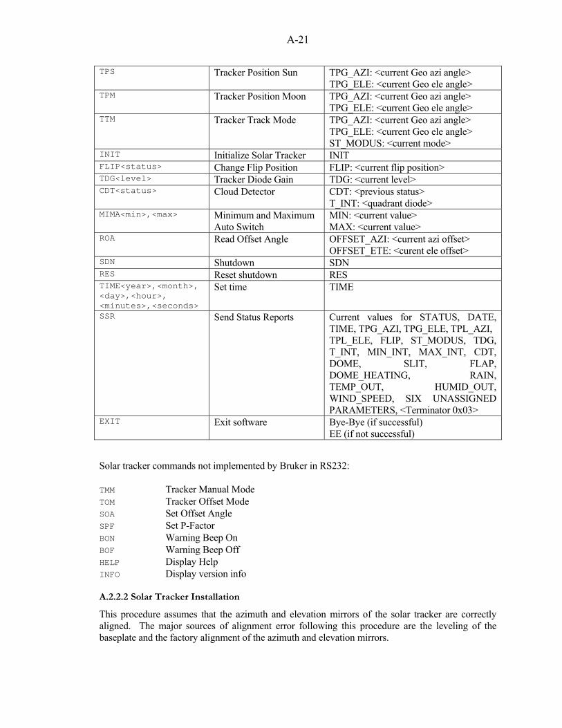
A-21

TPS Tracker Position Sun TPG_AZI: <current Geo azi angle> TPG_ELE: <current Geo ele angle>

TPM Tracker Position Moon TPG_AZI: <current Geo azi angle> TPG_ELE: <current Geo ele angle>

TTM Tracker Track Mode TPG_AZI: <current Geo azi angle> TPG_ELE: <current Geo ele angle> ST_MODUS: <current mode>

INIT Initialize Solar Tracker INIT FLIP<status> Change Flip Position FLIP: <current flip position> TDG<level> Tracker Diode Gain TDG: <current level> CDT<status> Cloud Detector CDT: <previous status>

T_INT: <quadrant diode> MIMA<min>,<max> Minimum and Maximum

Auto Switch MIN: <current value> MAX: <current value>

ROA Read Offset Angle OFFSET_AZI: <current azi offset> OFFSET_ETE: <curent ele offset>

SDN Shutdown SDN RES Reset shutdown RES TIME<year>,<month>, <day>,<hour>, <minutes>,<seconds>

Set time TIME

SSR Send Status Reports Current values for STATUS, DATE, TIME, TPG_AZI, TPG_ELE, TPL_AZI, TPL_ELE, FLIP, ST_MODUS, TDG, T_INT, MIN_INT, MAX_INT, CDT, DOME, SLIT, FLAP, DOME_HEATING, RAIN, TEMP_OUT, HUMID_OUT, WIND_SPEED, SIX UNASSIGNED PARAMETERS, <Terminator 0x03>

EXIT Exit software Bye-Bye (if successful) EE (if not successful)

Solar tracker commands not implemented by Bruker in RS232: TMM Tracker Manual Mode TOM Tracker Offset Mode SOA Set Offset Angle SPF Set P-Factor BON Warning Beep On BOF Warning Beep Off HELP Display Help INFO Display version info A.2.2.2 Solar Tracker Installation

This procedure assumes that the azimuth and elevation mirrors of the solar tracker are correctly aligned. The major sources of alignment error following this procedure are the leveling of the baseplate and the factory alignment of the azimuth and elevation mirrors.

A-22

1. To install the new solar tracker, first carefully level it. Remove the CaF2 window from the roof. 2. Enter the correct latitude, longitude, pressure, and temperature in c:/soltr227/strack.cfg. 3. Set the time and date of the suntracker computer using an accurate clock and the DOS "date" command. 4. Remove the source input tube of the IFS125 and place a flat mirror on the floor and level it. Alternatively, an oil dish can be used. Start the soltr227.exe software. Set TOM to center the returning solar beam on itself, making the beam vertical. 5. Replace the CaF2 window in the roof. 6. Put the solar tracker into TPS mode. Replace the source input tube and physically move the IFS125 to align the input tube directly under the incoming solar beam. Work quickly. 7. Adjust the 45 degree input tube mirror to center the solar beam on the flat entrance mirror in source compartment. 8. Adjust the flat entrance mirror in the source compartment to center the beam on the off-axis parabolic mirror. 9. Adjust the off-axis parabolic mirror in the source compartment, to center the beam exactly on the 4 mm field stop (4 mm is the approximate size of the solar image). 10. Use TTM and adjust the rectangular quadrant detector mirror so that in TTM mode, the solar beam is exactly centered on the 4 mm field stop.

A-23

A.2.3 Telescope Dome

Technical Innovations – Robodome Jerry Smith 7851 Cessna Avenue Gaithersburg, MD 20879 www.homedome.com Tel: 301-977-9000 Fax: 301-977-1106 Email: [email protected] Description:

The Robodome consists of an electronics control box which controls a fiberglass telescope dome. The dome has motors for rotation and shutter. The dome can rotate infinitely in azimuth. The shutter motor circuit is completed by bronze loops that make electrical contact with the shutter motor only at the dome's "home" position. The dome's azimuth position is sensed by an inexpensive light sensor that is positioned over a plastic disk with six holes. As the dome rotates, the plastic disk rotates and the light sensor produces a square wave. The dome electronics board counts the light sensor edges and compares this to the calibrated circumference of the dome to determine the current azimuth position. The dome's shutter position is sensed using limit switches at the top and bottom of shutter travel. The schematic diagram and other useful information are in the dome manual. The OPEN/CLOSE/CW/CCW buttons on the hand control operate the motors directly, through two relays. The two relays and two motors give four possible combinations (OPEN/CLOSE/CW/CCW). The “HOME” button of the hand control requires operation of the main microprocessor on the dome’s electronics board. The serial connection to the Hercules computer also requires operation of the main microprocessor on the dome’s electronics board. For this reason, the “HOME” button of the hand control will not work while the data acquisition software is running. The GINF dome information string is stored in src/config/site/README.site in the CVS archive, in case of mishaps. Connection to Hercules Computer:


From Hercules computer: qtalk –m /dev/ser2 To see what you are typing, turn on echo: <CTRL>A; e To quit qtalk: <CTRL>A; q Communication Protocol:

Write Line Separator: None Write Terminator: None

A-24

Read Terminator: CR Serial Port: COM1 Baud Rate: 9600 Data Bits: 8 Stop Bits: 1 Parity: No Protocol: None

A.2.3.1 Dome Direct RS232 Commands:

The dome will not accept commands in lowercase letters. GINF - Get Info Sample Reply: V4,228,223,2,223,0,2,1,0,220,227,0,128,255,255,255,255,255,255,255,999,1,0 (25 parameters describing current dome status) Gxxx - Go to Azimuth position xxx in degrees Sample Reply for 15 degree turn: RP1 (R for clockwise or L for counter-clockwise) P2 (Pnnnn updates of azimuth tick values as dome turns) V4,228,223,2,8,0,2,0,1,220,227,0,128,255,255,255,255,255,255,255,999,1,0 GHOM - Go to Home Sample Reply: LP7 (format similar to Gxxx) P6 (Pnnnn updates of azimuth tick values as dome turns) V4,228,223,2,224,0,2,1,0,220,227,0,128,255,255,255,255,255,255,255,999,1,0 GTRN - Training Sequence (Dome turns clockwise to home and then makes a full turn back to home. Records HOME position, circumference, and coasting in memory.) Sample Reply: P4 P5 (Pnnnn updates of azimuth tick values as dome turns) V4,229,9,2,8,0,2,1,0,6,12,0,128,255,255,255,255,255,255,255,999,1,0 GOPN - Shutter Open Sample Reply: OSZ18 SZ19 (SZnn updates as shutter moves) V4,228,223,2,224,0,2,1,0,220,227,0,128,255,255,255,255,255,255,255,999,1,0 GCLS - Shutter Close Sample Reply: CSZ22 SZ22 (SZnn updates as shutter moves) V4,228,223,2,224,0,1,1,0,220,227,0,128,255,255,255,255,255,255,255,999,1,0 GTST - Test Data No Reply: Should be 6 parameters for ADC values

A-25

A.2.4 Weather Station

Coastal Environmental Systems – Zeno 3200 820 First Avenue South Seattle, WA 98134 www.coastalenvironmental.com Tel: 206-682-6048 Fax: 206-682-5658 Email: [email protected] Description:

The Zeno weather station consists of commercial weather sensors connected to a datalogger. The datalogger contains the conversion parameters for each of the weather sensors. The datalogger outputs the sensor values as a string over RS232 at 1 Hz. In Darwin and Lamont, we have added an RS232 optical line isolation unit, to prevent lightning damage. The datalogger contains a battery and charger, and is plugged directly into the AC container power. This means that the weatherstation and datalogger are fully isolated from the Hercules computer, in case of a lightning strike. The weatherstation configuration file is stored in src/config/site/README.site in the CVS archive, in case of mishaps. Connection to Hercules Computer:


From Hercules computer: qtalk –m /dev/ser3 To quit qtalk: <CTRL>A; q Administrator Password: zeno A.2.4.1 Direct RS232 Commands:

The Zeno data is continually output as a comma-delimited string at 1 Hz. Data format: DATE TIME WSPD WDIR W_GUST W_SD AT RH SR BARO RAIN WETNESS VBATT BIT To interrupt this output and enter the user menus: "U" <enter> See the Zeno manual for more details. Total data logging memory: 127420 Max # of records: 4550 Size of each data record: 28 A.2.4.2 Barometric Pressure (S1080Z)

Manufacturer: Setra (Model 270) Units: hPa Accuracy: 0.3 hPa from -29 °C to +54 °C Testing: Periodic comparison to mercury manometer.

A-26

Principle: Ceramic capsule that deforms with pressure. The capacitance between gold electrodes on the inside surface of the capsule varies proportionally with applied pressure. A.2.4.3 Relative Humidity and Air Temperature (S1276Z)

Manufacturer: Vaisala (Humitter 50) Units: °C and % RH Accuracy: ±3% RH; ±0.1°C (0°C to +70°C); ±0.2°C (-30°C to +60°C) Testing: Compared to calibrated lab RTD at 23.07°C for parkfalls_ifs1 RH not fully tested. parkfalls_ifs1 reports 98 – 100 % when fully saturated. Principle: RH – Hygroscopic capacitative. Capacitance of thin film sensor varies with humidity. Temperature – Thermistor. Small bead of semiconducting material whose resistance varies nonlinearly with temperature change. A.2.4.4 Wind Speed and Direction (S1146Z)

Manufacturer: R.M. Young Company (Model 03002 Wind Sentry) Units: m s-1 and degrees Accuracy: Not indicated Testing: Verified that wind speed changed with rotation of sensor. Verified that wind direction varied approximately correctly with direction. Principle: Wind speed – Magnetically induced AC voltage produced by rotating magnet on cup shaft. Wind direction – Conductive potentiometer with 10K ohm resistance A.2.4.5 Pyranometer (S1114Z)

Manufacturer: Li-Cor (Model LI-200SZ) Units: W m-2 Accuracy: ±5% in natural daylight Testing: Verified that sensor values changed when exposed to light. Did not calibrate. Principle: Silicon photovoltaic detector; converts light directly to current. A.2.4.6 Precipitation Detector (S1391Z)

Manufacturer: Environmental Technology, Inc. (Model ES-1) Units: Yes/No Accuracy: NA Testing: Verified that sensor correctly indicates presence of rain. Principle: Presence of water changes either capacitance or resistance (not clear which) of grid. The snow sensor has been connected in parallel with the rain sensor to detect all precipitation. A.2.4.7 Leaf Wetness Sensor (S1169)

Manufacturer: Davis Units: 1 – 15 Accuracy: NA Testing: Verified that sensor correctly indicates presence of wetness. Principle: Detection of electrical resistance between gold-plated elements of grid. A.2.4.8 Mercury Manometer

Manufacturer: Princo Instruments (453 Weather Service Barometer) Units: mm Hg

A-27

Testing: Purchased as an absolute calibration standard, with NIST-traceable calibration certificate. Principle: Fortin mercury manometer. The mercury manometer is not connected to the Zeno datalogger. It is read manually.

A-28

A.2.5 Other laboratory instrumentation

A.2.5.1 NTP-GPS Receiver

Model: Masterclock – NTP100-GPS 2484 W Clay St Saint Charles, MO 63301-2548 www.masterclock.com Tel: 800-940-2248 Email: [email protected] Connection to Hercules Computer:

Network 192.168.1.106 Direct Communication:

Telnet to 192.168.1.106 A.2.5.2 Network Camera

Stardot Technologies – Netcam 6820 Orangethorpe Ave, Building H Buena Park, CA 90620 www.stardot-tech.com Tel: 888-782-7368 Fax: 714-228-9283 Email: [email protected] Description:

The Stardot Netcam is a small network camera with a fisheye lens that is mounted on the roof of the laboratory. The Netcam operating system is Linux and it is possible to reach the Netcam directly using telnet, if troubleshooting is required. Connection to Hercules Computer:


Use web browser to connect to 192.168.1.107:8080 A.2.5.3 Scroll Pump

Varian Inc. – TriScroll 300 121 Hartwell Avenue Lexington, MA 02421 www.varianinc.com Tel: 800-882-7426 Fax: 781-860-5437 Email: [email protected]

A-29

Description:

8.8 cfm dry scroll pump with an ultimate pressure of 1.3 x 10-2 hPa. One repair kit and one maintenance kit is located at Caltech Connection to Hercules Computer:

Optical Fiber Power is controlled by an optical fiber which is driven digitally Direct Communication:

The pump is simply "on-off". It can be turned on and off from ifsdoit: > Power Pump On > Power Pump Off

A.2.5.4 Scroll Pump Pressure Sensor

Park Falls: Wenzel Electronics – Micropirani Wenzel Electronics was purchased by MKS and no longer exists. Darwin, Lamont: MKS – 925C Micropirani MKS Instruments 90 Industrial Way, Wilmington, Massachusetts 01887 www.mksinst.com Tel: 800-227-8766 (in the USA), Fax: 978-284-4999 Description:

The Micropirani is a thermal conductivity gauge measuring in the range of 10-5 hPa to 103 hPa. The Wenzel Electronics and MKS Micropirani sensors are operationally similar, but have a different pinout for power and signal on their DB-9 connectors. To accommodate this change, we modified the cable between the Hercules computer and MKS Micropirani sensor so that it is no longer one-to-one. Connection to Hercules Computer:

9-pin analog cable Direct Communication:

The Micropirani pressure sensor is completely passive and does not accept commands.

A-30

A.2.6 Network and Communication

A.2.6.1 Network Information

Network Hardware

Park Falls: 16-port network switch Darwin and Lamont: Linksys BEFsx41 router

Network Assignments

All network devices (except the Hercules computer) have the username "admin". Address Device 192.168.1.1 Programmable Router 192.168.1.101 IFS125 192.168.1.102 IFS125 Workstation 192.168.1.103 QNX Hercules2 Computer 192.168.1.104 QNX Hercules Computer 192.168.1.105 UPS-BD Web/SNMP Card 192.168.1.106 NTP100-GPS 192.168.1.107 StarDot Network Camera 192.168.1.109 Norton PPP dialup A.2.6.2 Modem

US Robotics – 56K V.92 External Faxmodem www.usr.com Connection to Hercules Computer:


From Hercules computer: qtalk –m /dev/ser4 To quit qtalk: <CTRL>A; q

A-31

A.2.7 Power Systems

A.2.7.1 Uninterruptible Power Supply

Powerware – 9120 with ConnectUPS BD Network Card 8609 Six Forks Road Raleigh, NC 27615 www.powerware.com Tel: 1-800-356-5794 Email: [email protected] Description:

The Powerware 9120 is a 1500 W UPS. The installed network card allows it to be monitored on the network. Connection to Hercules Computer:


Use web browser to connect to 192.168.1.105

A-32

A.2.8 Digital and analog inputs/output signals

The digital and analog communication with the Hercules computer is designed by Jean-Francois Blavier and summarized here. A.2.8.1 Control Using Digital Lines

The Hercules port A is used in output mode to control the following subsystems:

Bit Assignment Values 0 IFS125 power 0 = Off; 1 = On 1 Modem power 0 = Off; 1 = On 2 Suntracker power 0 = Off; 1 = On 3 Dome power 0 = Off; 1 = On 4 Pump power 0 = Off; 1 = On 5 IFS125 reset 0 = Normal; 1 = Reset 6 Unused 7 Unused

The output of port A is not directly connected to the subsystem control. Instead an on-board latch is used to sample the value of port A. The latch is updated on the rising edge of bit 0 of port E. This was done to retain the power status of the various subsystems across computer resets. The Hercules port B is used in input mode to read the contents of the latch. The correct way to modify one bit of the latch is to first read the full byte on port B, change the bit in the read value, write the modified value to port A, finally toggle bit 0 of port E. A.2.8.2 Monitoring of Analog Inputs

Assignment of 32 ADC Channels Channel Units Description 0 Temperature (°C) Computer, disks 1 Temperature (°C) Computer, center 2 Temperature (°C) IFS125 motor compartment 3 Temperature (°C) IFS125 scanner compartment 4 Temperature (°C) IFS125 interferometer compartment 5 Temperature (°C) IFS125 detector compartment 6 Temperature (°C) IFS125 source compartment 7 Temperature (°C) IFS125 input tube 8 Temperature (°C) IFS125 laser cover 9 Temperature (°C) IFS125 electronics box 10 Temperature (°C) Suntracker leveling plate 11 Temperature (°C) Suntracker azimuth assembly 12 Temperature (°C) Suntracker elevation assembly 13 Temperature (°C) Pump motor 14 Temperature (°C) Pump body 15 Temperature (°C) Zeno weatherstation datalogger 16 Temperature (°C) Container air 17 Voltage (V) Main 24 VDC 18 Voltage (V) Heat 15 VDC 19 Voltage (V) Unswitched 12 VDC

A-33

20 Voltage (V) Switched 12 VDC 21 Voltage (V) Computer 5 VDC 22 Voltage (V) Dome 15 VDC 23 Voltage (V) Laser 12 VDC 24 Voltage (V) Micropirani +12 VDC 25 Voltage (V) Micropirani -12 VDC 26 Current (A) Main 24 VDC 27 Current (A) Heat 15 VDC 28 Current (A) Unswitched 12 VDC 29 Current (A) Dome 15 VDC 30 Current (A) Laser 12 VDC 31 Voltage (V) Micropirani pressure sensor

The system is used in single-ended mode (differential mode would yield only 16 channels). Because we have one negative voltage to monitor and because we need to properly measure values near zero, all inputs are operated in bipolar mode. The temperature sensors (LM235A) have an output which is directly proportional to the absolute temperature: Vout = 10 mV / K. With a ±5 V input range, the ADC transfer function will be: (32768DN / 5V) * (0.01V / K) = 65.536 DN/K The system is designed to operate over a wide range for the "Main 24 V" and "Heat 15 V". The voltage sensing is done through a divide by 4 resistor network. This allows for a ±40 V sensing range. Most other voltages ("Unswitched 12 V", "Switched 12 V", "Dome 15 V", "Laser 12 V", "MicroPirani +12 V", and "MicroPirani -12 V") are sensed through a divide by 2 network, for a range of ±20 V. The lonely "Computer 5 V" is sent directly to the ADC input, for a range of ±10 V. The current sensors have part numbers LTS15-NP for "Main 24 V", LTS25-NP for "Heat 15 V", and LTS6-NP for "Unswitched 12 V", "Dome 15 V", and "Laser 12 V", with the following transfer functions: Vout = 2.500 + 0.0428 * Iin (for "Main 24 V") Vout = 2.503 + 0.0254 * Iin (for "Heat 15 V") Vout = 2.501 + 0.1064 * Iin (for "Unswitched 12 V") Vout = 2.496 + 0.1096 * Iin (for "Laser 12 V") Vout = 2.506 + 0.1080 * Iin (for "Dome 15 V") A.2.8.3 Reference and Background Information

1. The latch in the digital control is needed because some subsystems take a long time to stabilize (e.g. the laser). Although we don't expect the computer to be reset often, it is good to avoid a 20 minutes wait after each computer reset.

A-34

2. The "Laser power" control and "Laser 12 V" monitor were originally designed to operate the laser because it is a critical component and is easily modified for DC-operation. This feature has since been renamed “Modem” and has been modified to control power to the network devices. 3. The LM235A have an accuracy of 1°C from -40°C to +125°C. (i.e., an accuracy of 1 K from 233 K to 398 K). 4. The "Computer, disks" sensor is used to control the fan in the computer box. The "IFS125HR, scanner compartment" and "IFS125HR, interferometer compartment" are used to control heaters on the instrument. The "Suntracker, azimuth assembly" and "Pump, motor" temperature sensors are also used to servo heaters. These controls run autonomously. 5. A temperature reading of 0 K indicates a short-circuit in the wiring. Whereas an over-range reading indicates a disconnected sensor (7.5 V for the servoed sensors and 12.3 V for all others, but these will be outside the ±5 V range). 6. The dividers for voltage sensing were done with DIP resistors network which were selected for a good match between individual resistors. The accuracy should be better than 0.5%. 7. The "Unswitched 12 V" is produced by a Vicor DC/DC converter which powers the Hercules. It is set for 12.5 V to better meet the Hercules and disk drives requirements. The "Switched 12 V" and "Computer 5 V" are outputs from the Hercules

A-35

A.2.9 Laboratory structure

A.2.9.1 Container

Ken Martin Martin Container Inc. 1400 S. Atlantic Ave. Compton, CA 90221-0185 USA www.container.com Tel: (800) 221-3727, 310-638-6000 Fax: 310-638-0025 Email: [email protected]

A.2.9.2 Heater – Air Conditioner Unit

Fedders "Y Chassis" (parkfalls_ifs1 and lamont_ifs3) Fedders Corporation http://www.fedders.com/catalog/appliances/roomac/fed_y.htm# Connection to Hercules Computer:

Heater-AC is not connected to the Hercules computer. Direct Communication:

There is no direct communication with the heater-AC.

Temperature Setpoint During Power Outages

Park Falls – The heater/AC control panel in Park Falls is powered by +5 VDC. We modified the control panel so that it receives its +5 VDC input from a power converter connected to the UPS. This prevents the heater/AC settings from being lost during power outages. Only the control panel is connected to the UPS, not the heater/AC itself. Darwin – The AC control panel in Darwin contains a battery. This prevents the AC settings from being lost during power outages.

A-36

A.3 Data Acquisition Software

A.3.1 Data Acquisition Software Overview

The devices described previously are all monitored and/or controlled with a Diamond Systems Hercules board and an additional control board. As mentioned previously, the Hercules board includes four serial ports, used for communication with the solar tracker, telescope dome, weatherstation, and modem. The Hercules board includes 32 wide-range analog inputs for monitoring temperatures, voltage, currents, and pressure of the scroll pump. Five digital I/O lines of the Hercules board are used to command power to the solar tracker, telescope dome, modem, IFS125, and IFS125 reset line. The IFS125, network camera, NTP-GPS satellite time receiver, and uninterruptible power supply are commanded within the local area network. The operating system of the Hercules computer is QNX, with custom data acquisition software written by Norton Allen. The data acquisition software continuously acquires data from the laboratory devices, over the serial, analog, digital, and network connections. All of this data is saved as binary telemetry data at 1 Hz, 0.5 Hz, or 0.125 Hz. There are a few exceptions. The Stardot Netcam files are saved directly as jpg files and the IFS125 interferograms are saved as “slices” in the original binary format. On the Hercules computers, the source code is stored in /home/citco2/src. The executables are distributed to /home/citco2/bin. Zhonghua Yang’s overnight analysis code is in /home/citco2/src/dp. Past overnight analysis emails are stored in /home/citco2/anal. Data currently being written is saved to /data/citco2. After that data is processed by reduce, it is saved in a yymmdd directory, in /data/citco2/raw/flight. The automated data acquisition is defined in src/TM/IFS.tma. Throughout the night, the acquisition software records weather and housekeeping data. When the calculated solar elevation angle reaches 0°, the scroll pump is commanded on and the FTS is evacuated to 0.5 hPa. Following the pumping sequence, the telescope dome opens and the solar tracker points to the calculated solar ephemeris. If the solar intensity is sufficient (~45 W m-2), the solar tracker begins active tracking of the sun and the FTS begins acquisition of solar interferograms. The specific acquisition parameters, including the field stop diameter, detector gains, scanner velocity, and optical path difference, are set in src/site/IFSopts.pm. Throughout the scan, the solar intensity measured by the solar tracker quadrant sensor is recorded at 0.5 Hz. Since only spectra acquired under stable solar intensity are suitable for atmospheric retrievals, the standard deviation of the solar intensity is later used to evaluate spectral quality. Forward and reverse interferograms are analyzed separately to maximize the number of unobstructed scans. Acquisition of solar interferograms continues as long as the solar intensity is sufficient for active tracking of the sun. If the weather station detects rain, then the telescope dome closes and spectral acquisition ceases until weather conditions improve. When the calculated solar elevation reaches 0° at the end of the day, the telescope dome is closed. Each night, interferograms recorded during the day are copied onto a removable hard disk. Overnight analysis software performs a Fourier transform to produce spectra from the interferograms, fits narrow HCl lines to verify the instrument lineshape, and calculates preliminary atmospheric column retrievals. These results are then emailed to Pasadena to monitor performance. At two month intervals, the removable hard disk is manually replaced with an empty one. The full disk is mailed to Pasadena for analysis and archiving. The operational data rate is ~50 GB month-1. The documentation below includes a description of the data acquisition source code files, a list of all telemetry data which is acquired, an explanation of the data directory structure, a list of

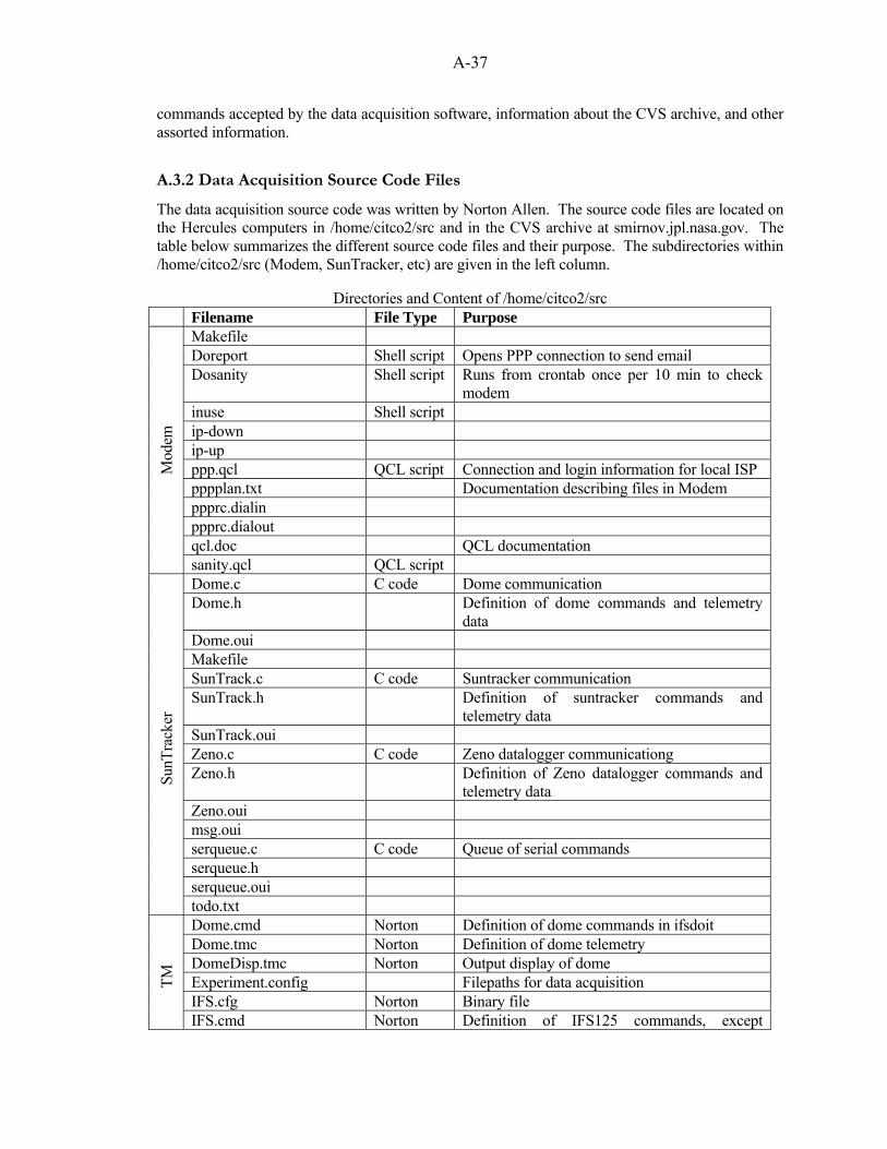
A-37

commands accepted by the data acquisition software, information about the CVS archive, and other assorted information.

A.3.2 Data Acquisition Source Code Files

The data acquisition source code was written by Norton Allen. The source code files are located on the Hercules computers in /home/citco2/src and in the CVS archive at smirnov.jpl.nasa.gov. The table below summarizes the different source code files and their purpose. The subdirectories within /home/citco2/src (Modem, SunTracker, etc) are given in the left column.

Directories and Content of /home/citco2/src

Filename File Type Purpose Makefile Doreport Shell script Opens PPP connection to send email Dosanity Shell script Runs from crontab once per 10 min to check

modem inuse Shell script ip-down ip-up ppp.qcl QCL script Connection and login information for local ISP pppplan.txt Documentation describing files in Modem ppprc.dialin ppprc.dialout qcl.doc QCL documentation

Mod

em

sanity.qcl QCL script Dome.c C code Dome communication Dome.h Definition of dome commands and telemetry

data Dome.oui Makefile SunTrack.c C code Suntracker communication SunTrack.h Definition of suntracker commands and

telemetry data SunTrack.oui Zeno.c C code Zeno datalogger communicationg Zeno.h Definition of Zeno datalogger commands and

telemetry data Zeno.oui msg.oui serqueue.c C code Queue of serial commands serqueue.h serqueue.oui

SunT

rack

er

todo.txt Dome.cmd Norton Definition of dome commands in ifsdoit Dome.tmc Norton Definition of dome telemetry DomeDisp.tmc Norton Output display of dome Experiment.config Filepaths for data acquisition IFS.cfg Norton Binary file

TM

IFS.cmd Norton Definition of IFS125 commands, except

A-38

“direct” commands IFS.pcm Norton Verbose description of entire telemetry

dataframe IFS.spec Norton Contains information used by appgen to create

Makefile IFS.tbl Norton Defines console display appearance ITS.tma Norton Main data acquisition algorithm IFS2.tbl Norton Defines console 2 display appearance IFSDiag.tmc Norton Determines whether IFS125 diagnostics are

“OK” or “fail” IFSctrl Norton IFSloop Norton Loop to initiate overnight analysis and then

restart ifsdoit IFSq.c C code IFS125 command queue IFSq.oui Norton IFSq.pm Norton IFS125 command queue parameters IFSretr Norton Retrieves sliced data files from IFS125 IFSretr.pm Norton IFS125 retrieval parameters IFStm.pm Norton ModemPower.c C code README.TM.txt ST.cmd Norton Contains suntracker commands for ifsdoit ST.edf Norton Unused telemetry extraction format for

suntracker ST.tmc Norton Definition of suntracker telemetry SW.cmd Norton Contains software commands, such as “Email

Report” SZA.tmc Norton Definition of Sol_ele telemetry VERSION Contains current version number Zeno.cmd Norton Definition of Zeno datalogger commands for

ifsdoit Zeno.edf Norton Unused extraction format for Zeno datalogger Zeno.tmc Norton Definition of Zeno datalogger telemetry base.tmc Norton Definition of IFS125 telemetry catalog PERL Parses IFSretr.log and extracts list of first slice

from each scan cceng.edf Unused telemetry extraction format cceng1.edf Telemetry extraction format cceng2.edf Second part of telemetry extraction format cmdstat.tmc Definition of power latch telemetry display.cfg fields.cfg herc_ad.c C code ADC inputs herc_ad.h herc_ad.oui herc_ad.tmc Definition of ADC telemetry herc_dio.c C code DIO inputs herc_dio.oui herc_hndlr.c

A-39

hercules.cmd Hercules DIO commands idler.tmc idlercol.tmc ifs.doit info.tmc Telemetry extraction format for info files infoext.h infoext.oui interact modem.txt Readme file for modem and network devices pb.doit solpos.c C code Calculate solar position in horizon coordinates solpos.h solpos.tmc sza_calc.c C code Calculate solar zenith angle sza_calc.h szatest.c tm.dac todo.txt Norton todo list (old) Makefile OpusHdr bin2csv Converts binary telemetry data to comma

separated variables csv Directory Contains bin2csv output definitions exam.ksh Shell script Spectral fitting analysis ifsreduce Shell script Overnight data processing, invokes exam.ksh

anal

slice-ipp Directory Contains slice-ipp source code IFSopts.pm IFS125 data acquisition parameters (scanner

velocity, etc.) Makefile READ.site Text containing laboratory details and backup

files boot doreport.pm Recipient list for emails etc Backup of QNX system files flimit.ipp Spectral file limits required by slice-ipp herc_cal.tmc Calibration curves for current sensors and

Micropirani location.h Latitude, longitude, and altitude of container

site preamps.h IFS125 addressing of each detector slice-ipp.in Input file for slice-ipp overnight analysis slice-ipp.top Input file for slice-ipp overnight analysis

conf

ig/si

te_s

ubdi

rect

ory

strack.cfg Backup of suntracker configuration file. This file must be physically copied to the suntracker computer.

The TM/Config subdirectory should be a soft-link to the appropriate instrument/location directory under Bruker/config (e.g. ln -s ../config/parkfalls_ifs1 Config).

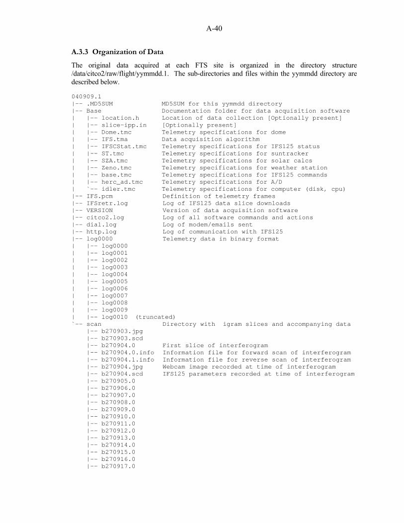
A-40

A.3.3 Organization of Data

The original data acquired at each FTS site is organized in the directory structure /data/citco2/raw/flight/yymmdd.1. The sub-directories and files within the yymmdd directory are described below. 040909.1 |-- .MD5SUM MD5SUM for this yymmdd directory |-- Base Documentation folder for data acquisition software | |-- location.h Location of data collection [Optionally present] | |-- slice-ipp.in [Optionally present] | |-- Dome.tmc Telemetry specifications for dome | |-- IFS.tma Data acquisition algorithm | |-- IFSCStat.tmc Telemetry specifications for IFS125 status | |-- ST.tmc Telemetry specifications for suntracker | |-- SZA.tmc Telemetry specifications for solar calcs | |-- Zeno.tmc Telemetry specifications for weather station | |-- base.tmc Telemetry specifications for IFS125 commands | |-- herc_ad.tmc Telemetry specifications for A/D | `-- idler.tmc Telemetry specifications for computer (disk, cpu) |-- IFS.pcm Definition of telemetry frames |-- IFSretr.log Log of IFS125 data slice downloads |-- VERSION Version of data acquisition software |-- citco2.log Log of all software commands and actions |-- dial.log Log of modem/emails sent |-- http.log Log of communication with IFS125 |-- log0000 Telemetry data in binary format | |-- log0000 | |-- log0001 | |-- log0002 | |-- log0003 | |-- log0004 | |-- log0005 | |-- log0006 | |-- log0007 | |-- log0008 | |-- log0009 | |-- log0010 (truncated) `-- scan Directory with igram slices and accompanying data |-- b270903.jpg |-- b270903.scd |-- b270904.0 First slice of interferogram |-- b270904.0.info Information file for forward scan of interferogram |-- b270904.1.info Information file for reverse scan of interferogram |-- b270904.jpg Webcam image recorded at time of interferogram |-- b270904.scd IFS125 parameters recorded at time of interferogram |-- b270905.0 |-- b270906.0 |-- b270907.0 |-- b270908.0 |-- b270909.0 |-- b270910.0 |-- b270911.0 |-- b270912.0 |-- b270913.0 |-- b270914.0 |-- b270915.0 |-- b270916.0 |-- b270917.0

A-41

|-- b270918.0 |-- b270919.0 |-- b270920.0 |-- b270921.0 |-- b270922.0 |-- b270923.0 First slice of interferogram |-- b270923.0.info Information file for forward scan of interferogram |-- b270923.1.info Information file for reverse scan of interferogram |-- b270923.jpg Webcam image recorded at time of interferogram |-- b270923.scd IFS125 parameters recorded at time of interferogram |-- b270924.0 |-- b270925.0 |-- b270926.0 |-- b270927.0 |-- b270928.0 |-- b270929.0 |-- b270930.0 |-- b270931.0 |-- b270932.0 |-- b270933.0 |-- b270934.0 |-- b270935.0 |-- b270936.0 |-- b270937.0 |-- b270938.0 |-- b270939.0 |-- b270940.0 |-- b270941.0 (truncated) |-- mail.log Log of emails sent [Optionally present] |-- sanity.log Log of modem heartbeat monitor [Optionally present] |-- saverun.log Log indicating shutdown procedure |-- tm.dac Binary file specifying telemetry frame |-- TM Directory of ascii telemetry files |-- 051022.1_1a.csv 1 Hz ascii telemetry files, labels in 1st row |-- 051022.1_1b.csv 1 Hz ascii telemetry files, labels in 1st row |-- 051022.1_1c.csv 1 Hz ascii telemetry files, labels in 1st row |-- 051022.1_1d.csv 1 Hz ascii telemetry files, labels in 1st row |-- 051022.1_2.csv 1/2 Hz ascii telemetry files, labels in 1st row |-- 051022.1_8.csv 1/8 Hz ascii telemetry files, labels in 1st row During Oct 2005, we added a sub-directory within each yymmdd directory which is named "TM". "TM" contains comma-delimited text files with telemetry data. Apart from this addition in Oct 2005, every yymmdd directory has an identical structure to the one shown above. The files which are necessary for processing the data are IFSretr.log and the contents of the scan directory.

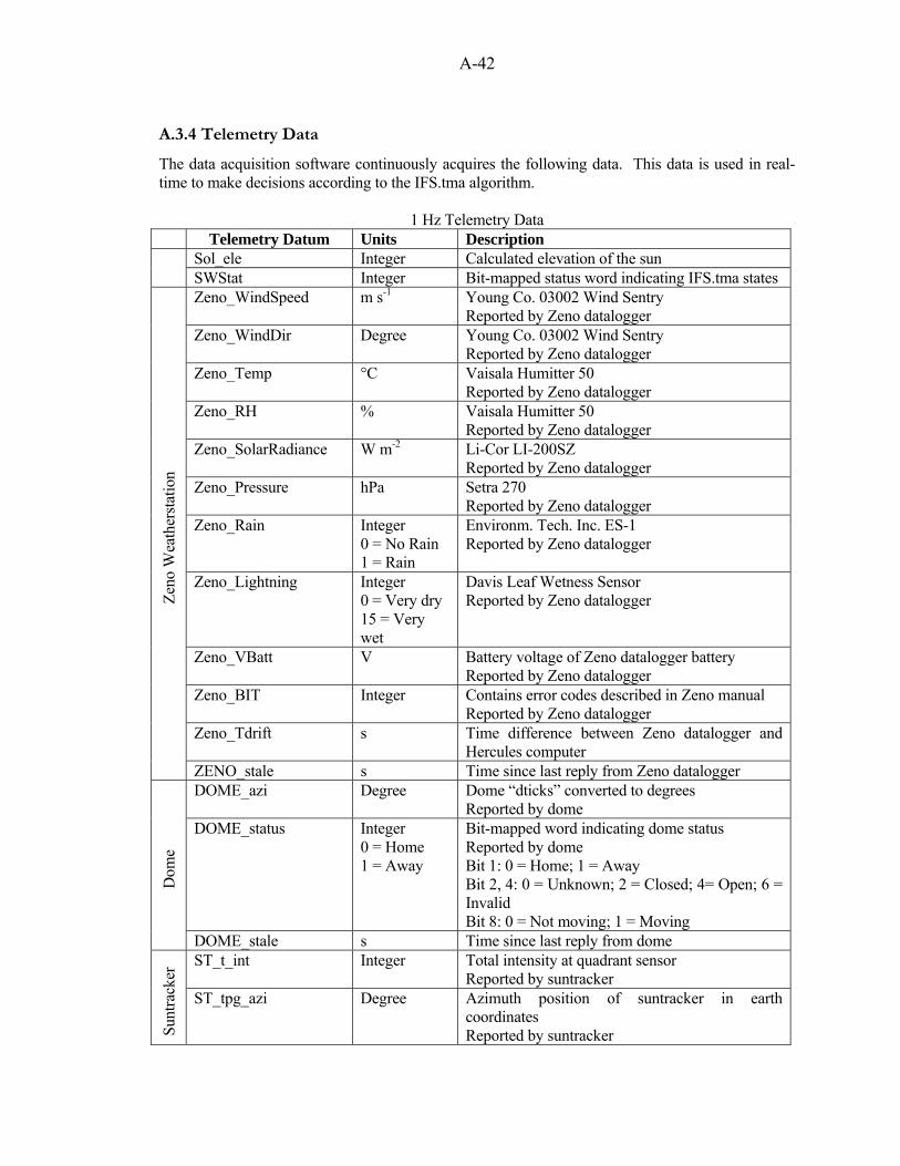
A-42

A.3.4 Telemetry Data

The data acquisition software continuously acquires the following data. This data is used in real-time to make decisions according to the IFS.tma algorithm.

1 Hz Telemetry Data Telemetry Datum Units Description

Sol_ele Integer Calculated elevation of the sun

SWStat Integer Bit-mapped status word indicating IFS.tma states Zeno_WindSpeed m s-1 Young Co. 03002 Wind Sentry

Reported by Zeno datalogger Zeno_WindDir Degree Young Co. 03002 Wind Sentry

Reported by Zeno datalogger Zeno_Temp °C Vaisala Humitter 50

Reported by Zeno datalogger Zeno_RH % Vaisala Humitter 50

Reported by Zeno datalogger Zeno_SolarRadiance W m-2 Li-Cor LI-200SZ

Reported by Zeno datalogger Zeno_Pressure hPa Setra 270

Reported by Zeno datalogger Zeno_Rain Integer

0 = No Rain 1 = Rain

Environm. Tech. Inc. ES-1 Reported by Zeno datalogger

Zeno_Lightning Integer 0 = Very dry 15 = Very wet

Davis Leaf Wetness Sensor Reported by Zeno datalogger

Zeno_VBatt V Battery voltage of Zeno datalogger battery Reported by Zeno datalogger

Zeno_BIT Integer Contains error codes described in Zeno manual Reported by Zeno datalogger

Zeno_Tdrift s Time difference between Zeno datalogger and Hercules computer

Zeno

Wea

ther

statio

n

ZENO_stale s Time since last reply from Zeno datalogger DOME_azi Degree Dome “dticks” converted to degrees

Reported by dome DOME_status Integer

0 = Home 1 = Away

Bit-mapped word indicating dome status Reported by dome Bit 1: 0 = Home; 1 = Away Bit 2, 4: 0 = Unknown; 2 = Closed; 4= Open; 6 = Invalid Bit 8: 0 = Not moving; 1 = Moving

Dom

e

DOME_stale s Time since last reply from dome ST_t_int Integer Total intensity at quadrant sensor

Reported by suntracker

Sunt

rack

er

ST_tpg_azi Degree Azimuth position of suntracker in earth coordinates Reported by suntracker

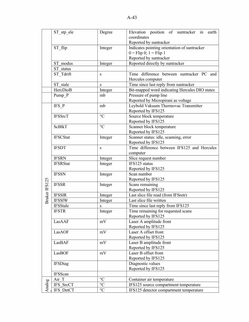
A-43

ST_stp_ele Degree Elevation position of suntracker in earth coordinates Reported by suntracker

ST_flip Integer Indicates pointing orientation of suntracker 0 = Flip 0; 1 = Flip 1 Reported by suntracker

ST_modus Integer Reported directly by suntracker ST_status ST_Tdrift s Time difference between suntracker PC and

Hercules computer ST_stale s Time since last reply from suntracker

HercDioB Integer Bit-mapped word indicating Hercules DIO states Pump_P mb Pressure of pump line

Reported by Micropirani as voltage IFS_P mb Leybold Vakuum Thermovac Transmitter

Reported by IFS125 IFSSrcT °C Source block temperature

Reported by IFS125 ScBlkT °C Scanner block temperature

Reported by IFS125 IFSCStat Integer Scanner status: idle, scanning, error

Reported by IFS125 IFSDT s Time difference between IFS125 and Hercules

computer IFSRN Integer Slice request number IFSRStat Integer IFS125 status

Reported by IFS125 IFSSN Integer Scan number

Reported by IFS125 IFSSR Integer Scans remaining

Reported by IFS125 IFSSlR Integer Last slice file read (from IFSretr) IFSSlW Integer Last slice file written IFSStale s Time since last reply from IFS125 IFSTR Integer Time remaining for requested scans

Reported by IFS125 LasAAF mV Laser A amplitude front

Reported by IFS125 LasAOF mV Laser A offset front

Reported by IFS125 LasBAF mV Laser B amplitude front

Reported by IFS125 LasBOF mV Laser B offset front

Reported by IFS125 IFSDiag Diagnostic values

Reported by IFS125

Bru

ker I

FS12

5

IFSScan Air_T °C Container air temperature IFS_SrcCT °C IFS125 source compartment temperature

Ana

log

It

IFS_DetCT °C IFS125 detector compartment temperature

A-44

IFS_IntCT °C IFS125 interferometer compartment temperature IFS_ScnCT °C IFS125 scanner compartment temperature IFS_MtrCT °C IFS125 motor compartment temperature IFS_InpTT °C IFS125 input tube temperature IFS_LaserT °C IFS125 laser cover temperature Zeno_T °C Zeno datalogger temperature IFS_ElecT °C IFS125 electronics box temperature PC_CtrT °C Hercules computer temperature PCDiskT °C Hercules computer disk temperature Pump_BdyT °C Pump body temperature Pump_MtrT °C Pump motor temperature ST_AziT °C Suntracker azimuth temperature ST_EleT °C Suntracker elevation temperature ST_LvlPT °C Suntracker leveling plate temperature Laser_12I A Current sensor Dome_15I A Dome current USx_12I A Unswitched 12 VDC current Hear_15I A Heater current Main_24I A Main 24 VDC current uP_M12V V uP_P12V V Laser_12V V Dome_15V V Dome 15 VDC PC_5V V Hercules 5 VDC Sw_12V V Switched 12 VDC USw_12V V Unswitched 12 VDC Heat_15V V Heater 15 VDC

Ana

log

Inpu

ts

Main_24V V Main 24 VDC

0.5 Hz Telemetry Data

Telemetry Datum Units Description CPUst % Hercules CPU usage MEMst DISKst Disk1st Disk2st H

ercu

les

Disk3st

0.25 Hz Telemetry Data Telemetry Datum Units Description

ST_off_azi Degree Offset between TTM and TPS solar pointing values Reported by suntracker

ST

ST_off_ele Degree Offset between TTM and TPS solar pointing values Reported by suntracker

A-45

A.3.5 Quick Command Tree for ifsdoit

This is a quick list to identify commands which are accepted by the data acquisition software. The letters which are capitalized must be typed. The others will be finished by command completion. Dome Close shutter Exit Goto xxx Home Open shutter EMail Error Report Warning EXit IFs Aerosol Cell Direct Exit IDlescan INsbidlescan ReAd status RePeat Aerosol Cell IDlescan INsbidlescan ReSet Hw Assert Release Sw SEt preamp gains x x SHortSolar SOlar SOlar Insb Timesynch Log "string" Power Dome ON OFf Ifs125hr ON OFf Modem ON OFf Pump ON OFf Suntracker ON OFf Quit SAvelog "string" SUntracker

A-46

Clouddetector OFf ON Exit Flip 0 1 Goto x x Init SLeep SYnchronize time Track By diode To programmed sun position SW status Calculate solar elevation Hold ReAd file ReInit SEt SHutdown Completely Instantly Quickly SImulate sunRise sunSet Timewarp Telemetry Logging Suspend Restart Start Zeno exit

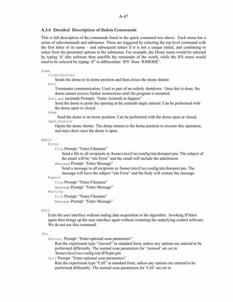
A-47

A.3.6 Detailed Description of ifsdoit Commands

This is full description of the commands listed in the quick command tree above. Each menu has a series of subcommands and submenus. These are triggered by selecting the top level command with the first letter of its name – and subsequent letters if it is not a unique initial, and continuing to select from the presented options in the submenus. For example, the Dome menu would be selected by typing ‘d’ (the software then autofills the remainder of the word), while the IFS menu would need to be selected by typing ‘if” to differentiate ‘IFS’ from ‘IOMODE’. Dome

Close shutter Sends the dome to its home position and then closes the dome shutter

Exit Terminates communication. Used as part of an orderly shutdown. Once this is done, the dome cannot receive further instructions until the program is restarted.

Goto xxx (azimuth Prompt): “Enter Azimuth in degrees” Send the dome to point the opening at the azimuth angle entered. Can be performed with the dome open or closed.

Home Send the dome to its home position. Can be performed with the dome open or closed.

Open shutter Opens the dome shutter. The dome returns to the home position to execute this operation, and stays there once the dome is open.

EMail

Error File Prompt: “Enter Filename”

Send a file to all recipients in /home/citco2/src/config/site/doreport.pm. The subject of the email will be “site Error” and the email will include the attachment.

Message Prompt: “Enter Message” Send a message to all recipients in /home/citco2/src/config/site/doreport.pm. The message will have the subject “site Error” and the body will contain the message.

Report File Prompt: “Enter Filename”

Message Prompt: “Enter Message” Warning

File Prompt: “Enter Filename” Message Prompt: “Enter Message” EXit

Exits the user interface without ending data acquisition or the algorithm. Invoking IFSdoit again then brings up the user interface again without restarting the underlying control software. We do not use this command.

IFs

Aerosol Prompt: “Enter optional scan parameters” Run the experiment type “Aerosol” in standard form, unless any options are entered to be performed differently. The normal scan parameters for ‘Aerosol’ are set in /home/citco2/src/config/site/IFSopts.pm

Cell Prompt: “Enter optional scan parameters” Run the experiment type “Cell” in standard form, unless any options are entered to be performed differently. The normal scan parameters for ‘Cell’ are set in

A-48

/home/citco2/src/config/site/IFSopts.pm Direct Prompt: “Enter Direct Parameters”

Sends a direct Bruker web interface command to the IFS. See alternative list for IFS125 acronyms. Three letter acronyms must be capitalized The allowed TLAs that can be sent to the IFS are defined in IFSopts.pm.

Exit Terminates communication. Used as part of an orderly shutdown.

IDlescan Prompt: “Enter Optional Scan Parameters” Run the experiment type “IdleScan” in standard form, unless any options are entered to be performed differently. The normal scan parameters for ‘IdleScan’ are set in /home/citco2/src/config/site/IFSopts.pm

ReAd status Reads IFS parameters (Diagnostics, Laser, IFS boxes on main screen)

RePeat Not operational.

ReSet HW

Assert Release

SW SEt preamp gains x x Prompt: “Enter Binary Gain Index for InGaAs and Si” SHortCell Prompt: “Enter Optional Scan Parameters”

Run the experiment type “ShortCell” in standard form, unless any options are entered to be performed differently. The normal scan parameters for ‘ShortCell’ are set in /home/citco2/src/config/darwin_ifs2/IFSopts.pm

SHortSolar Prompt: “Enter Optional Scan Parameters” Run the experiment type “ShortSolar” in standard form, unless any options are entered tobe performed differently. The normal scan parameters for ‘ShortSolar’ are set in /home/citco2/src/config/site/IFSopts.pm

SOlar Prompt: “Enter optional scan parameters” Run the experiment type “Solar” in standard form, unless any options are entered to be performed differently. The normal scan parameters for ‘Solar’ are set in /home/citco2/src/config/site/IFSopts.pm

SOlar Insb Time synch

Synchronizes the time between the Hercules computer and the IFS125 (sets IFS time to be that of the Hercules, as it is correct via using the NTP server)

IOmode

Changes the auto-completion option of the user interface. It can be set to never auto-complete. LOG Prompt: “Enter String to Log To Memo” Power

Dome OFf Turns the robodome power off ON Turns the robodome power on

Ifs125hr OFf Turns the IFS125 power off ON Turns the IFS125 power on

Modem OFf Turns the 12V power distribution box power off

A-49

ON Turns the 12V power distribution box power on Pump

OFf Turns the pump power off ON Turns the pump power on

SunTracker OFf Turns the sun tracker power off ON Turns the sun tracker power on

Quit

Ends software control of the instrument (shutting down both the data acquisition/control and the user interface), but does not attempt any shutdown of devices. The 'SW Shutdown' commands are preferred in normal operation.

SAvelog Prompt: “Enter Log Message”

Saves the logs – prompting a separate scanset. Appropriate to use after a failure. Note that it will trigger another processing run, and a second yymmdd directory.

SUntracker

Cloud detector – Not used. Exit

Terminates communication. Used as part of an orderly shutdown. Flip

0 Go to sun tracker flip state 0 1 Go to sun tracker flip state 1

Goto xxx (azimuth angle), Elevation Angle Send the sun tracker to the azimuth/elevation coordinates entered. E.g. SunTracker GoTo 0 -72 send the tracker to azi=0, ele=-72.

Init SLeep

Send the sun tracker to the sleep position. SYnchronize Time Track

By diode Start Tracker Track Mode (TTM), with corrections performed by the quadrant diode to center the sun on the input sample tube.

To programmed Moon position

Send the tracker so the mirrors are pointed to the calculated moon position (TPM) Sun position

Send the tracker so the mirrors are pointed at the calculated sun position (TPS) SW status

Calculate solar elevation Hold

Stop automatic runs and hold in a standard configuration. Note that this causes the dome to shut. It then allows the user to enter manual commands with no interference from IFS.tma.

ReAd file Reads commands from the text file /data/citco2/IFS.tmas. This command is superfluous, because the algorithm reads from this file every 15 seconds. Commands can be written to this file and they will be executed within 15 seconds. If the commands are to be executed only once, the file should end with "Validate ReadFile_Delete;" To loop, you can include "Validate ReadFile;" If neither of these options is used, the ReadFile partition will stop at

A-50

the end of the file, and an explicit "SW Status Read File" command will have to be issued on the console to re-execute the file.

The syntax of IFS.tmas is the same as the contents of a single State{} within a normal .tma file without any C-code (stuff in curly braces). e.g.:

> Dome Home +10 > Dome Open +30 > Dome GoTo Azimuth 102 Validate ReadFile_Delete;

You can't "hold until", but it is possible to "hold;" in conjunction with another partition.

ReInit Reinitialize communications with all connected devices, and restart the automated software run.

SEt prompt: “Enter Integer (Decimal: 123, Hex: 0x123F, Octal: 0123)” All of the SW status commands are implemented by setting the SWstatus variable to a specific value. This command exposes the underlying mechanism.

SHutdown Completely Instantly

Shuts down without waiting for the IFS to become idle. Quickly

Waits until the IFS125 becomes idle (i.e. the end of the next scan) before shutting down and exiting.

SImulate sunRise

Simulates the procedure for when the solar elevation becomes greater than 0 at sunrise. This is done by steadily increasing the solar elevation angle by 1 degree at a time. Good for testing that the software behaves as it should at this time, without having to wait until the next morning. Equivalent to the wake up procedure.

sunSet Simulates the procedure for when the solar elevation becomes less than 0 at sunset. This is done by decreasing the solar elevation angle by 1 degree at a time through 0 degrees. Also good for testing software behavior. Equivalent to the bedtime procedure.

Time warp Provides a means for testing algorithms with long time-sequences. A 30-minute delay can be written: Hold until ( SWstatus == SWS_TIMEWARP ) or 30:00; Then issuing the time warp command will jump ahead.

Telemetry Logging Resume Suspend

Use of this command is frowned upon since it makes it impossible to reconstruct the exact state of the machine from the data log.

Start Issued once automatically by the algorithm to get things going. Never required interactively.

Zeno Exit

Terminates communication. Used as part of an orderly shutdown. Other Notes:

A-51

There is no way to restart the automation after a failure without first exiting the software. Therefore, after a failure, type: > SaveLog Failure Shutdown

A-52

A.3.7 Routine monitoring of the data acquisition

For routine monitoring, it is necessary to monitor the weather and to respond to "error" emails. Actively monitoring the weather

Check weather each day. If winds are predicted to be >= 25 mph or if severe storms are predicted, then put the data acquisition in hold. To put the container in hold:

If the data acquisition is left in hold for more than 48 hours without running ‘reduce,’ it will cause an error in the binary data extraction. Connect to the Hercules computer. Use the commands sudo ditto -k /dev/con1 > SW Status Hold There will be no more Wakeup, Play, etc. The data acquisition will sit and wait, logging telemetry data. Check that the dome status is "Close" <CTRL>E then q to exit ditto To return to normal data acquisition:

Connect to the Hercules computer. Then: sudo ditto -k /dev/con1 > SW Status ReInit <CTRL>E then q to exit ditto Error Emails

A few places to look for clues, if there is an "error" email: $ tail /data/citco2/citco2.log - to see the most recent events in the log Look at netcam jpg - check to see if opening of dome is aligned with the shadows cast by the sun

A-53

A.3.8 Queuing directories to repeat the overnight analysis

Sometimes the overnight analysis is interrupted. It can be queued to begin again from scratch, after sunset. In the comments at the top of /home/citco2/bin/anal/ifsreduce: # Analysis script to run under reduce as: # Analysis='bin/anal/ifsreduce background $analdir $directory' Here $directory refers to the raw data directory and $analdir refers to the analysis directory where the log file is located. In interactive use, it works like this: run=050201.1 analdir=/home/citco2/anal/$run directory=/data/citco2/raw/flight/$run cd /home/citco2 bin/anal/ifsreduce background $analdir $directory To start the processing immediately, replace the last line with: BEDTIME=yes bin/anal/ifsreduce background $analdir $directory A.3.9 Hercules Computer Shutdown Instructions

1. Type "sudo shutdown -b", then your password. 2. When QNX says it is safe to turn power off, flip power switch on main 28 V supply. The computer is now running on batteries. 3. Unplug the battery cable at the main 28 V supply. The computer is now turned off. 4. Turn heater power supply off. Follow these in reverse to bring the system back up Remember to turn the 28 V power supply back on. Otherwise, the computer will run fine until the batteries are dead.

A-54

A.3.10 Useful QNX Commands

QNX system files:

/var/log/syslog /etc/resolv.conf - contains DNS information /etc/ntp.conf - contains NTP information /etc/config/sysinit.4 - contains time zone information

QNX commands and processes:

sin info System CPU and RAM usage sin tree System processes sin files System files sin -P perl files Reveals file current perl script is reading sin fd who Shows who is logged in use command Help for command sudo shutdown Restart system sudo shutdown –b Shutdown system QNX utilities:

qtalk -m /dev/serX/ Terminal emulation program <CTRL>A; x Qtalk menu options (x to exit) ditto /dev/conX Echo QNX screen on local computer <ctrl>E; q Ditto menu options (q to exit)

Other details:

Manual extraction of info files: extract /data/citco2/raw/flight/040331.1 'infoext –d /data/citco2/raw/flight/040331.1' Manual extraction of other telemetry files: extract /data/citco2/raw/flight/yymmdd.1 cceng1ext If IFS.tma runs for several days without ‘reduce’, then 'extract' will get stuck during the next time it is run. It will produce garbled error messages. To end the processes which are stuck: slay memo slay rdr or find the offending process with ps –ef and then use “kill -9”

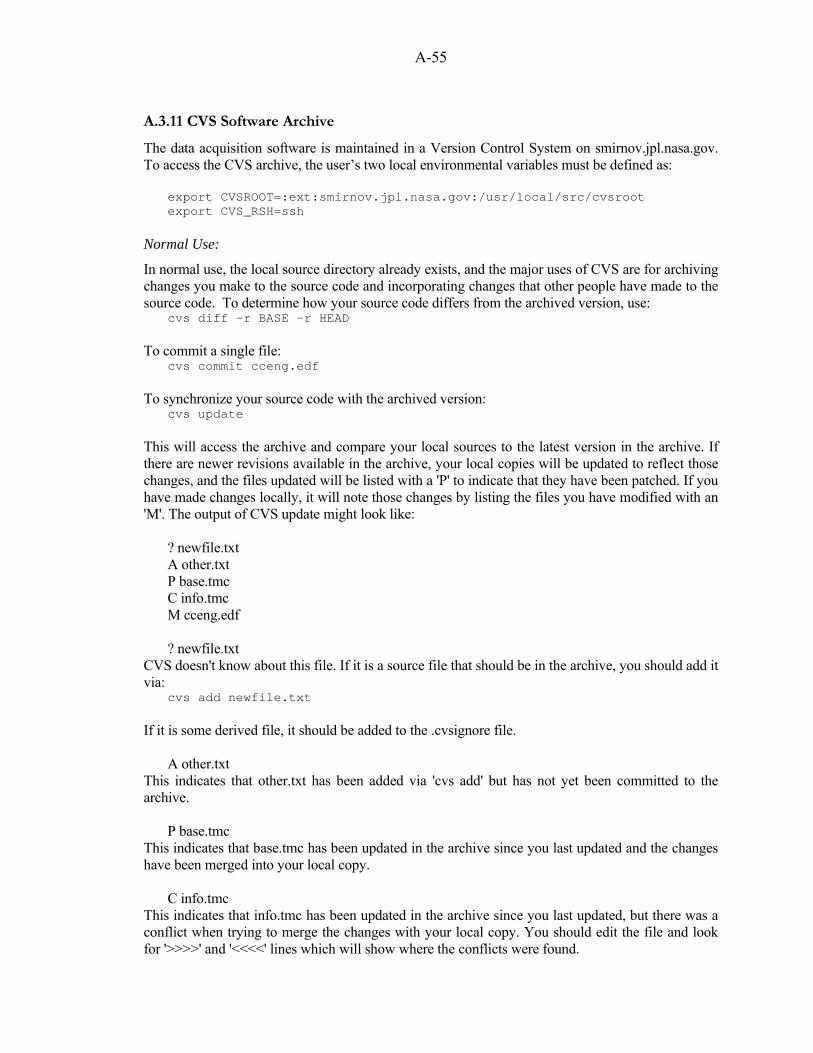
A-55

A.3.11 CVS Software Archive

The data acquisition software is maintained in a Version Control System on smirnov.jpl.nasa.gov. To access the CVS archive, the user’s two local environmental variables must be defined as: export CVSROOT=:ext:smirnov.jpl.nasa.gov:/usr/local/src/cvsroot export CVS_RSH=ssh Normal Use:

In normal use, the local source directory already exists, and the major uses of CVS are for archiving changes you make to the source code and incorporating changes that other people have made to the source code. To determine how your source code differs from the archived version, use: cvs diff -r BASE -r HEAD To commit a single file: cvs commit cceng.edf To synchronize your source code with the archived version: cvs update This will access the archive and compare your local sources to the latest version in the archive. If there are newer revisions available in the archive, your local copies will be updated to reflect those changes, and the files updated will be listed with a 'P' to indicate that they have been patched. If you have made changes locally, it will note those changes by listing the files you have modified with an 'M'. The output of CVS update might look like: ? newfile.txt A other.txt P base.tmc C info.tmc M cceng.edf ? newfile.txt CVS doesn't know about this file. If it is a source file that should be in the archive, you should add it via: cvs add newfile.txt If it is some derived file, it should be added to the .cvsignore file. A other.txt This indicates that other.txt has been added via 'cvs add' but has not yet been committed to the archive. P base.tmc This indicates that base.tmc has been updated in the archive since you last updated and the changes have been merged into your local copy. C info.tmc This indicates that info.tmc has been updated in the archive since you last updated, but there was a conflict when trying to merge the changes with your local copy. You should edit the file and look for '>>>>' and '<<<<' lines which will show where the conflicts were found.

A-56

M cceng.edf This indicates that cceng.edf has been modified in the local directory, but the changes have not been committed. Once you have done and update and resolved any issues, you will probably want to commit your changes to the archive. Generally we like to commit changes after we've determined that the changes work, but sometimes it makes sense to commit changes so they can be accessed on other systems even though they are still under active development. To commit your changes, you can issue: cvs commit which will commit all changes in the current directory subtree, or: cvs commit cceng.edf which will commit changes in cceng.edf only. To check out the source code for the first time: cvs checkout -d src Bruker

A-57

A.4 Data Transfer, Archive, and Processing

Due to the limitations of our network connections in Park Falls and Darwin, it is necessary to physically transfer data by disk. Once at Caltech, the data is copied to the RAID and to archive disks. The .MD5SUM of each copy is verified to make sure no data corruption has occurred. The sliced interferograms are Fourier transformed using software by Jean-Francois Blavier. The following sections describe the removable disks, the Caltech RAID, the slice-ipp software, the filenaming convention, and some other assorted information.

A.4.1 Removable Disks

General Information

The Hercules computer contains two disks: a permanent (or fixed) disk and a removable disk. Both disks are 200 GB Western Digital EIDE disks. Due to limitations of the QNX4 filesystem, the formatted capacity of the disks is only 137 GB. The removable disk is mounted in Storcase DE-90 disk carrier. Each night, ifsreduce makes a copy of the day's data on the removable disk. When the fixed disk is ~100 GB full, we exchange the removable disk for an empty one. After the data from the removable disk has been transferred to permanent storage at Caltech/JPL, that data is deleted from the fixed disk. Instructions for swapping the removable disk

IFSloop has to be stopped in order to unmount the disk, but it can be restarted after the disk is unmounted, and the physical swap can happen during normal data acquisition. Unmount the disk remotely. This requires exiting and restarting IFSloop: > SW Shutdown Quickly sudo umount /dev/hd1.1t77 sudo umount /dev/hd1.1 IFSloop On site: 1. Unpack the cardboard box. The removable hard disk is in the black plastic case. This removable disk is the "empty" one. The main computer is sitting on the folding table and has all the labels and blinking lights. The removable disks are inserted into the bay in the bottom right corner of the front panel. 2. There is a key in the front of the removable drive bay. Turn it clockwise one quarter turn. 3. Wait for the removable drive bay LEDs to stop blinking in opposition. This takes about 10 seconds. 4. Raise the handle of the "full" removable drive and gently pull it out. 5. Place the new "empty" drive from Pasadena in the bay. Make sure it is fully seated. 6. Turn key counter-clockwise one quarter turn.

A-58

7. Wait for LEDs to stop blinking in opposition. 8. Put the "full" removable into the anti-static bag. Put it into the black plastic case and pack it back into the cardboard box. 9. The mailing address is: Mail Stop 150-21 Caltech 1200 E. California Blvd. Pasadena, CA 91125 Remount the disk remotely. This does not require exiting IFSloop: sudo mount -p /dev/hd1.1 sudo mount /dev/hd1.1t77 /removable]

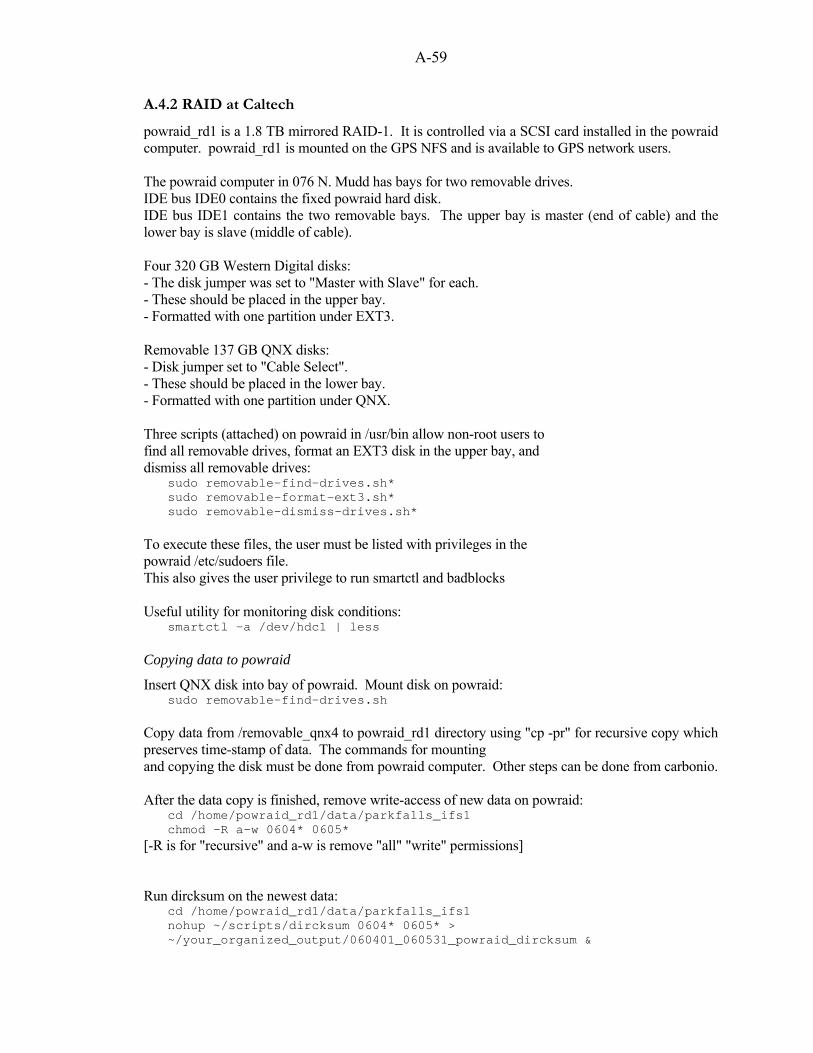
A-59

A.4.2 RAID at Caltech

powraid_rd1 is a 1.8 TB mirrored RAID-1. It is controlled via a SCSI card installed in the powraid computer. powraid_rd1 is mounted on the GPS NFS and is available to GPS network users. The powraid computer in 076 N. Mudd has bays for two removable drives. IDE bus IDE0 contains the fixed powraid hard disk. IDE bus IDE1 contains the two removable bays. The upper bay is master (end of cable) and the lower bay is slave (middle of cable). Four 320 GB Western Digital disks: - The disk jumper was set to "Master with Slave" for each. - These should be placed in the upper bay. - Formatted with one partition under EXT3. Removable 137 GB QNX disks: - Disk jumper set to "Cable Select". - These should be placed in the lower bay. - Formatted with one partition under QNX. Three scripts (attached) on powraid in /usr/bin allow non-root users to find all removable drives, format an EXT3 disk in the upper bay, and dismiss all removable drives: sudo removable-find-drives.sh* sudo removable-format-ext3.sh* sudo removable-dismiss-drives.sh* To execute these files, the user must be listed with privileges in the powraid /etc/sudoers file. This also gives the user privilege to run smartctl and badblocks Useful utility for monitoring disk conditions: smartctl -a /dev/hdc1 | less Copying data to powraid

Insert QNX disk into bay of powraid. Mount disk on powraid: sudo removable-find-drives.sh Copy data from /removable_qnx4 to powraid_rd1 directory using "cp -pr" for recursive copy which preserves time-stamp of data. The commands for mounting and copying the disk must be done from powraid computer. Other steps can be done from carbonio. After the data copy is finished, remove write-access of new data on powraid: cd /home/powraid_rd1/data/parkfalls_ifs1 chmod -R a-w 0604* 0605* [-R is for "recursive" and a-w is remove "all" "write" permissions] Run dircksum on the newest data: cd /home/powraid_rd1/data/parkfalls_ifs1 nohup ~/scripts/dircksum 0604* 0605* > ~/your_organized_output/060401_060531_powraid_dircksum &

A-60

[~/scripts/dircksum is the path to where your copy of dircksum is saved] Check whether dircksum is finished by looking at output: cat ~/your_organized_output/060401_060531_powraid_dircksum When it is finished and you see that the dircksums agree, remove the QNX disk from powraid. Create EXT3 backup copies, by copying from RAID to EXT3 hard disks and run dircksum on the EXT3 copies.

A-61

A.4.3 MD5SUM tool: dircksum

dircksum is a stand-alone PERL script which generates an MD5SUM. During the overnight analysis, dircksum is run on the data directory on the fixed disk. The result is saved as .MD5SUM in that day's data directory. After the data is copied to the removable disk, dircksum is run again. If the result differs from .MD5SUM, then this is reported in the ifsreduce email. After receiving the removable disk at Caltech, is necessary to run dircksum on each copy that we make (there are three: the RAID and two Linux archive disks), to guarantee that there is no corruption. For example: nohup ~/scripts/dircksum /home/powraid_rd1/data/parkfalls_ifs1/050[8,9]* > powraid_050801_050905_dircksum & This will run dircksum on the new files and output a summary text file to powraid_050801_050905_dircksum. Then look at the text file to make sure there are no problems. More information about dircksum: $ use dircksum dircksum [ -w ] [ -o outputfile ] [-v] [-c] dir [ dir ... ] Generates a listing of CRCs of the contents of the directory and all its subdirectories. This file should be sensitive only to the file names and their contents, not to the dates and/or the order of the files in the directory. -w indicates that the results should be written to a file named .MD5SUM or .CKSUM in the target directory. If -w is not specified and .MD5SUM or .CKSUM exists, the current output is compared to that file and the differences are reported. If an output file is not specified with the -o flag, output may be written to a temp file. The temp file may not be removed if a comparison against the old .CKSUM shows a discrepancy. -c indicates the cksum program should be used to generate the hash. By default, and MD5 hash is used. -c is implicit when -w is not specified and a .CKSUM file exists. -v indicates that the results should be written to STDOUT in addition to any file specified via -w or -o or the temp file implicit if a .CKSUM file exists. If neither -w nor –o are specified and no .CKSUM file exists, -v is implicit.

A-62

A.4.4 Slice-IPP Fourier Transform Software

Explanation of three-digit version numbering for the code: X.Y.Z (e.g. slice-ipp 1.0.0): "X" is the software architecture number. "Y" is the major revision number. This number will change if the effect on the data will be significant. Examples of this would be corrections for the runs whose time info is affected by download stress or whose slices have been partly overwritten. When this number changes, some parts of the data set will need to be reprocessed. "Z" is the minor revision number. This is essentially for bug fix purposes. For example, supporting the third instrument might bring new problems which would otherwise not affect the Park Falls or Darwin data. A.4.4.1 Fourier-Transform Using Slice-IPP

1a. Run the "catalog" program. The catalog program parses the contents of IFSretr.log and generates a list of the first slice from each interferogram. The syntax for catalog is this: catalog /home/powraid_rd1/data/parkfalls_ifs1/040909.1/IFSretr.log > 040909.1_catalog catalog can act on many directories at once: catalog /home/powraid_rd1/data/parkfalls_ifs1/04*/IFSretr.log > 04xxxx_catalog 1b. Concatenate slice-ipp.top and the catalog to create an input file named slice-ipp.in, which will be read by slice-ipp: cat slice-ipp.top 040909.1_catalog > slice-ipp.in The slice-ipp.top file is carefully documented, and indicates the data directory path, the spectra output path, and other parameters for the Fourier transform. These must be modified appropriately. 1c. Execute slice-ipp: ./slice-ipp | tee slice-ipp_040909_output.txt slice-ipp will read the slice-ipp.in file in the slice-ipp directory, and produce spectra. A.4.4.2 Bruker Acronyms contained in the IFS125 spectral headers

Acquisition Parameter Block AQM: Acquisition Mode COR: Correlation Test Mode DEL: Delay Before Measurement DLY: Stabilization Delay HFW: Wanted High Frequency Limit LFW: Wanted Low Frequency Limit NSS: Sample Scans

A-63

PLF: Result Spectrum RES: Resolution RGN: Signal Gain, Background SGN: Signal Gain, Sample TDL: To do list Data Parameter Block - Spectrum CSF: Y - Scaling Factor DAT: Date of Measurement DPF: Data Point Format FXV: Frequency of First Point MNY: Y – Minimum MXY: Y – Maximum NPT: Number of Data Points TIM: Time of Measurement Data Parameter Block - IgSm CSF1: Y - Scaling Factor DAT1: Date of Measurement DPF1: Data Point Format DXU1: X Units FXV1: Frequency of First Point LXV1: Frequency of Last Point MNY1: Y - Minimum MXY1: Y - Maximum NPT1: Number of Data Points TIM1: Time of Measurement Data Parameter Block - IgSm/2.Chn CSF2: Y - Scaling Factor DAT2: Date of Measurement DPF2: Data Point Format FXV2: Frequency of First Point LXV2: Frequency of Last Point MNY2: Y - Minimum MXY2: Y - Maximum NPT2: Number of Data Points TIM2: Time of Measurement FT Parameter Block APF: Apodization Function HFQ: End Frequency Limit for File LFQ: Start Frequency Limit for File PHR: Phase Resolution PHZ: Phase Correction Mode SPZ: Stored Phase Mode ZFF: Zero Filling Factor Instrument Parameter Block ABP: Absolute Peak Pos in Laser*2 AG2: Actual Signal Gain 2nd Channel ARS: Number of Background Scans ASG: Actual Signal Gain ASS: Number of Sample Scans DAQ: Data Acquisition Status DUR: Scan time (sec) FOC: Focal Length GBW: Number of Good BW Scans GFW: Number of Good FW Scans HFL: High Folding Limit

A-64

INS: Instrument Type LFL: Low Folding Limit LWN: Laser Wavenumber P2A: Peak Amplitude 2nd Channel P2K: Backward Peak Location 2nd Channel P2L: Peak Location 2nd Channel P2R: Backward Peak Amplitude 2nd Channel PKA: Peak Amplitude PKL: Peak Location PRA: Backward Peak Amplitude PRL: Backward Peak Location RDY: Ready Check RSN: Running Sample Number SSP: Sample Spacing Divisor Optic Parameter Block APT: Aperture Setting BMS: Beamsplitter Setting CHN: Measurement Channel DTC: Detector Setting HPF: High Pass Filter LPF: Low Pass Filter PGN: Preamplifier Gain SON: External Synchronization SRC: Source Setting VEL: Scanner Velocity Sample Parameter Block CNM: Operator Name EXP: Experiment IST: Instrument Status SFM: Sample Form SNM: Sample Name A.4.4.3 Additional Acronyms defined for the IFS125 spectral headers

Acquisition Parameter Block OPL: Optical path difference on the long side in cm OPS: Optical path difference on the short side in cm Instrument Parameter Block HUM: IFHum: (This became a Bruker item) IDA: IFSDT_avg ISS: ScanStatus(e.g. OK) PIM: IFS_P (This became a Bruker item) TLP: IFSSrcT (This became a Bruker item) TSC: ScBlkl_T (This became a Bruker item) Optic Parameter Block FOV: Field of view in mrad PGR: InGaAs_R or Si_R Sample Parameter Block ALT: Altitude DAA: Dome_azi_avg DSM: Dome_Status_max HOU: Zeno_RH_avg LAT: Latitude

A-65

LON: Longitude POU: Zeno_Press_avg SAA: ST_tpg_azi_avg SDA: ST_Tdrift_avg SEA: ST_tpg_ele_avg SFM: ScanType(e.g. Solar; this is a Bruker item with special use) SIA: ST_t_int_avg SIS: ST_t_int_std SOA: ST_off_azi_avg SOE: ST_off_ele_avg STM: ST_TPS_max TOU: Zeno_Temp_avg WDA: Zeno_WindDir_avg WDS: Zeno_WindDir_std WSA: Zeno_WindSpeed_avg WSM: Zeno_WindSpeed_max WSS: Zeno_WindSpeed_std ZLM: Zeno_Lightning_max ZRM: Zeno_Rain_max ZSA: Zeno_SolarRadiance_avg ZSS: Zeno_SolarRadiance_std ZVA: Zeno_VBatt_avg A.4.4.4 Filenaming Convention

Character Description Examples 1 Site c=Caltech; l=Lauder; p=Park Falls; d=Darwin 2 Instrument a=Park Falls 125HR; m=Lauder 120M; h=Lauder 120HR;

b=Darwin 125HR 3 – 6 Year 2003, 2004, 2005, etc 7 – 8 Month 01=January, 02=February, etc 9 – 10 Day 01, 02, 03,.....31 11 Source s=solar; m=moon; l=lamp; a=scattered sky 12 Cell 0=no cell; a, b, c, d=5 mbar HCl cells 13 Beamsplitter a=Caltech CaF2; b=Lauder CaF2, c=Darwin CaF2 14 Dichroic a=Caltech; b=Lauder; c=Darwin 15 Filter 0=no filter; a=red color glass; b=Germanium; c=interference 16 Detector a=InGaAs; b=Si, c=InSb, x=dual acquisition InGaAs+Si 17 “.” 18 – 21 Spectrum number 0000-9999 Example for Darwin: db20060101seccax.000 for dual-acquisition spectra db20060101secc0a.000 for InGaAs db20060101seccab.000 for Si db20060101secccc.000 for InSb

A-66

A.5 General Logistics

These sections describe logistic and site information specific to each of the laboratories. A.5.1 Contact Information and Account Numbers

Caltech Account Numbers:

POW.00019-1-JPL.1263534 / P424704 POW.00021-1-NASA.000154 / P432845 POW.00023-1-JPL.1269365FAB / P456526 Shipping Account Numbers:

DHL Inbound Account Number (Yael Yavin / Coleen Roehl): 968716818 DHL General Account Number (Yael Yavin / Coleen Roehl): 788486140 DHL: 1-800-225-5345 FedEx Account Number (Caltech): 100945223 Caltech Shared Computer Accounts:

Username its.caltech.edu: tccon Dial-up modem: 1-800-429-1113 or 626-685-7098 Caltech Campus Contact Information

Biology Stockroom, Pat Perrone: x4922 Central Engineering Stockroom, Corey Campbell: x4680, Moses X4720 Central Warehouse, Rick Germond: x4891 Electrical, Mike Anchondo: x4999 Glassblower, Rick Gerhart: x6518 Physics Machine Shop, Rick Paniagua: x6631 or x6641 RAID, David Kewley: x5767 Shipping and Receiving: x4893 Transportation: x4703/4 Telephone set up, Donna Sparks: x4735 Collaborator Contact Information

Gretchen Aleks: x6293, [email protected] Jean-Francois Blavier: 818-354-6665; [email protected] Geoff Toon: 818-354-8259; [email protected] Rebecca Washenfelder: x6894, [email protected] Paul Wennberg: x2447, [email protected] Zhonghua Yang: x6293; [email protected] Yael Yavin: x8552; [email protected]

A-67

A.5.2 Caltech FTS Site

A.5.2.1 Caltech Contact Information and Logistics

Location:

34.1342 N; 118.1261 W; 0.210 km Mailing Address:

California Institute of Technology 1200 E. California Blvd. OR 391 S. Holliston Ave. Pasadena, CA 91125 Container Access:

Container phone: 626-395-4662 A.5.2.2 Caltech Network Connectivity

TCP/IP Settings:

IP 131.215.199.42 Subnet 255.255.255.0 Gateway 131.215.199.254 DNS 131.215.139.100 NTP 131.215.254.252, 131.215.65.2, and 131.215.254.254 (ntp1.caltech.edu, ntp3.caltech.edu, and ntp4.caltech.edu) The Linksys router (192.168.1.1 on LAN) has the following settings: 22 -> 192.168.1.104 (Hercules3) 8080 -> 192.168.1.107 (Stardot)

A-68

A.5.3 Park Falls FTS Site

A.5.3.1 Park Falls Contact Information and Logistics

Location:

45.9448 N; 90.2732 W; 0.442 km Mailing Address:

WLEF-TV W4551 State Road 182 Park Falls, WI 54552 USA Contact Information:

Jeff Ayers, [email protected] Roger Strand, [email protected] WLEF Tel: 715-762-2611 Jeff Ayers home Tel: 715-762-2490 Cell: 715-661-0011 Email: [email protected]

Local dial-up access in Park Falls:

715-762-1230 username: ctx19141 Travel Logistics:

Super 8 1212 Hwy 13 South Park Falls, WI, 54552 US 715-762-3383 Super 8 has added free wireless access. www.suncountry.com Container Access:

Container phone: 715-762-8053 Natural Disasters:

The Park Falls site is at risk from giant ice chunks falling from the support cables of the WLEF tower. The laboratory is directly underneath the support cables. The container roof is reinforced with plywood, the heater/AC has a protective aluminum cover, and the dome has a unistrut cover. The aluminum cover of the unistrut protection must be moved forward at the end of October, so that the aluminum cover is flush with the steel structure on the northern edge. On March 1, the aluminum cover must be moved north by ~8”. On April 15, the aluminum cover must be moved completely to the north, so that it does not obstruct the solar beam.

A-69

A.5.3.2 Park Falls Network Connectivity

The Park Falls FTS experiment is only available by modem PPP connection. The phone number is 715-762-8053; username: wennppp. There are two methods for connecting: using your own modem or using smirnov.jpl.nasa.gov

Instructions using personal modem:

To configure a Windows computer, use the "Create a New Connection" dialogue and select a dial-up connection. From the Connection Properties Dialog: "Options": Uncheck "Prompt for name and password". "Security": Check "Show terminal window" in "Interactive logon and scripting" "Networking": Select "Internet Protocol (TCP/IP)". Select "Properties" and in the ensuing dialog choose "Obtain an IP address automatically"; Select "Advanced" and de-select the option "Use default gateway on remote network". Make connection. When it connects, you'll get a terminal window. Hit <Enter> and it will prompt you for a terminal type (which is moot because you're not in a terminal emulator, but you have to give it an answer it likes, so type 'ansi') then login as wennppp. After you've logged in, you should get a line of funny characters (seems to be spaces and parentheses... something like '( {{ [ [ { '. When you see that, select 'Done' and it should finish connecting. Then you can bring up an ssh connection. Instructions using smirnov.jpl.nasa.gov modem:

Jean-Francois Blavier has setup the PPP client on smirnov.jpl.nasa.gov to call the container. This makes it possible to reach the container from computers that don't have a modem but are connected to the Internet. You must have an account on smirnov to use this connection. 1. Use SSH to connect to smirnov. 2. To initiate the connection to the container, type: sudo ppp-go This will return immediately to the command prompt, but the computer is actually dialing and negotiating the link in the background. After a few seconds, you will see: Serial connection established. Using interface ppp0 Connect: ppp0 <--> /dev/modem not replacing existing default route to eth0 [137.78.163.1] local IP address 192.168.1.109 remote IP address 192.168.1.103

A-70

Occasionally, the connection to the container will fail, probably due to the poor quality of the phone line. In that case the message is: Connect script failed 3. You can log into the Hercules with: ssh hercules2 4. If your computer runs an X11 server and your SSH connection allows X11 tunneling, then you can simply run Netscape on smirnov and have the display sent to your local screen: netscape http://stardotcam:8080/netcam.jpg If you are not running an X11 server on your local computer, then you can download the webcam picture to your directory on smirnov: wget http://stardotcam:8080/netcam.jpg 6. When you are done with the connection, do: sudo ppp-stop The system will quickly respond with a message similar to: Terminating on signal 2. PPP link to [ppp0] terminated. Connection terminated. Connect time 16.3 minutes. Sent 15187 bytes, received 120233 bytes. Connect time 16.3 minutes. Sent 15187 bytes, received 120233 bytes. Don't forget this last step, or the connection to the container will stay up.

A-71

A.5.4 Darwin FTS Site

A.5.4.1 Darwin Contact Information and Logistics

Location:

12.425 S; 130.891 E; 0.030 km

Mailing Address:

SSU NT Bureau of Meteorology 525 Stuart Highway Winnellie, NT 0821 Australia Contact Information:

Rex Pearson, Lead Technician, [email protected] Troy Culgan, Technician Michael Alsop, Technician Gary Eckert, Technician Tel: 618-8947-3815 618-8984-4515 (workshop) 580-388-4083 (voice-over-IP) Local dial-up access in Darwin:

Opusnet Account 019-833-1111 Username: acrs.3 Access to TWP ARM instrumental data:

198.129.82.242 Username: Oper Travel Logistics:

Sky City, Darwin (has free ADSL access) Gilruth Avenue, Mindil Beach Darwin, NT Australia +61 8 8943 8888 www.skycitydarwin.com.au Alatai Apartments McMinn St (Cnr Finniss St) Darwin, NT Australia +61 8 8981 5188 / 1800 628 833 www.alataiapartments.com.au

A-72

Collaborators:

Nicholas Deutscher Work 02 4221 3196 Mobile 0421 992216 Home 02 4229 3973 Email [email protected] Natural Disasters:

Cyclones. Lightning strikes.

A.5.4.2 Darwin Network Connectivity

Unlike the Park Falls FTS laboratory, the Darwin FTS laboratory is available on the network. TCP/IP Settings:

IP 198.129.82.248 Subnet 255.255.255.240 Gateway 198.129.82.241 DNS 134.178.6.5 and 146.137.100.120 NTP 198.129.82.74 Local SMTP 198.129.82.242 Dick Eagan (sysadmin at ARM) has allowed all IP addresses on ports 22 (ssh), 80 (html), 8080 (html), 8008 (html), 25 (smtp), 42 (nameserver), 53 (domain), and 123 (ntp) to reach our IP address. The Linksys router (192.168.1.1 on LAN) has the following settings: Port forwarding: 80 -> 192.168.1.101 (IFS125) 22 -> 192.168.1.104 (Hercules1) 8080 -> 192.168.1.107 (Stardot) Packet filtering: 1. Smirnov Allow Incoming --- 137.78.163.184 ~ 184 TCP 80 ~ 80 2. Bruce Allow Incoming --- 130.130.56.126 ~ 126 TCP 80 ~ 80 3. --- Allow Outgoing --- --- ALL --- 4. DNS Allow Incoming --- 130.202.101.22 ~ 22 ALL --- 5. DNS2 Allow Incoming --- 146.137.100.120 ~ 120 ALL --- 6. NTP Allow Incoming --- 198.129.82.74 ~ 74 ALL --- 7. Deny_80_In Deny Incoming --- --- TCP 80 ~ 80 8. Allow_Incoming Allow Incoming --- --- ALL --- What the port forwarding and packet filtering means: - Incoming DNS and NTP are allowed. - Incoming ports 22, 80, and 8080 are forwarded. However: - Only Smirnov and Bruce are allowed to visit port 80 (IFS125). All other IP addresses are denied. We can use lynx or netscape on Smirnov or Bruce to view the IFS125 webpage. - Outgoing access is allowed, so we can use internet and network from inside the container.

A-73

- Incoming access is allowed. This is necessary for network access within the container, including ping. Remote administration of the router is disabled, because it uses unsecure "http" instead of "https"

COLUMN ABUNDANCES OF CARBON DIOXIDE AND ...api/deki/files/309/...keeping my Ph.D. on track and aimed...

Documents

Transcript of COLUMN ABUNDANCES OF CARBON DIOXIDE AND ...api/deki/files/309/...keeping my Ph.D. on track and aimed...