Color to gray conversions in the context of stereo matching

Machine Vision and Applications manuscript No.(will be inserted by the editor)

Color to gray conversions in the context of stereo matchingalgorithms.An analysis and comparison of current methods and an ad-hoctheoretically-motivated technique for image matching.

Luca Benedetti · Massimiliano Corsini · PaoloCignoni · Marco Callieri · Roberto Scopigno

Received: date / Accepted: date

Abstract This study tackles the image color to gray conversion problem. The aim was tounderstand the conversion qualities that can improve the accuracy of results when the gray-scale conversion is applied as a pre-processing step in the context of vision algorithms, andin particular dense stereo matching. We evaluated many different state of the art color tograyscale conversion algorithms. We also propose an ad-hoc adaptation of the most theoret-ically promising algorithm, which we call Multi-Image Decolorize (MID). This algorithmcomes from an in-depth analysis of the existing conversion solutions and consists of a multiimage extension of the algorithm by Grundland et al. [14] which is based on PredominantComponent Analysis. In addition, two variants of this algorithm have been proposed andanalyzed: one with standard unsharp masking and another with a chromatic weighted un-sharp masking technique [28] which enhances the local contrast as shown in the approachby Smith et al. [37]. We tested the relative performances of this conversion with respectto many other solutions, using the StereoMatcher test suite [34] with a variety of differentdatasets and different dense stereo matching algorithms. The results show that the overallperformance of the proposed Multi-Image Decolorize conversion are good and the reportedtests provided useful information and insights on how to design color to gray conversion toimprove matching performance. We also show some interesting secondary results such asthe role of standard unsharp masking vs. chromatic unsharp masking in improving corre-spondence matching.

Keywords color to grayscale conversion · dense stereo matching · dimensionalityreduction · 3D reconstruction · unsharp masking

This work was funded by the EU IST IP 3DCOFORM

Visual Computing LabIstituto di Scienza e Tecnologie della Informazione “A. Faedo”Area della Ricerca CNR di PisaVia G. Moruzzi n. 1, 56124 PisaTel.: +39-050-3152925Fax: +39-050-3152930E-mail: [email protected]: [email protected]: [email protected]: [email protected]: [email protected]

2

Fig. 1: Isoluminant changes are not preserved with traditional color to grayscale conversion.Converting a blueish text whose luminance matches that of the red background to grayscalecan result in a featureless image.

1 Introduction

This paper tackles the color to grayscale conversion of images. Our main goal was to under-stand what can improve the quality and the accuracy of results when the grayscale conver-sion is applied as a pre-processing step in the context of stereo and multi-view stereo match-ing. We evaluated many different state-of-the-art algorithms for color to gray conversionand also attempted to adapt the most promising algorithm (from a theoretical viewpoint),thus creating an ad-hoc algorithm that optimizes the conversion process by simultaneouslyevaluating the whole set of images.

Color to grayscale conversion can be seen as a dimensionality reduction problem. Thisoperation should not be undervalued, since there are many different properties that need tobe preserved. For example, as shown in Fig. 1, isoluminant color changes are usually notpreserved with commonly used color to gray conversions. Many conversion methods havebeen proposed in recent years, but mainly focusing on the reproduction of color images withgrayscale mediums. Perceptual accuracy in terms of the fidelity of the converted image isoften the only objective of these techniques. These kinds of approaches, however, are notdesigned to fulfill the needs of vision and stereo matching algorithms.

The problem of the automatic reconstruction of three-dimensional objects and environ-ments from sets of two or more photographic images is widely studied in Computer Vi-sion [17]: traditional methods are based on matching features from sets of two or more inputimages. While some approaches [34] use color information, only a few solutions are ableto take real advantage of the color information. Many of these reconstruction methods areconceptually designed to work on grayscale images in the sense that, sooner or later in theprocessing, for a given spatial location, the algorithm will only consider a single numericalvalue (instead of the RGB triple). Often, this single numerical value is the result of a simpleaggregation of color values.

While finding a good way to exploit complete RGB information in stereo matchingwould be interesting, we preferred to focus on the color to gray conversion. A better ex-ploitation of color information during the matching would need to be implemented for eachavailable matching algorithm in order to maximize its usefulness and to assess its soundness.In contrast, working on an enhanced color to gray conversion step could straightforwardlyimprove the performances of an entire class of existing and already well-known reconstruc-tion algorithms. In other words we followed a domain separation strategy, since we decou-pled the color treatment from the computer vision algorithm using a separate preprocessingstep for the aggregation of the data.

The aims of this work are twofold. Firstly, to provide a wide and accurate comparisonof the performance of existing grayscale techniques. Secondly, to develop a new conversiontechnique based on the existing one by analyzing the needs of matching algorithms.

In general, three approaches can be used to evaluate the correctness of different color tograyscale conversion algorithms:

3

– A perceptual evaluation, such as the one employed in Cadık’s 2008 article [8], is bestsuited for grayscale printer reproduction and other human-related tasks.

– An information theory approach could quantify the amount of information that is lostduring the dimensionality reduction; to the best of our knowledge there are no othersimilar studies in this context.

– An approach that is tailored to measure the results of the subsequent image processingalgorithms.

We use the third approach, by evaluating the effectiveness of different grayscale conver-sions with respect to the image-based reconstruction problem. We chose a well-known classof automatic reconstruction algorithms, i.e., dense stereo matching [34] and we tested theperformance of the traditional color approach compared to many different conversion algo-rithms. In dense stereo matching, in order to compute 3D reconstructions, the correspon-dence problem must first be solved for every pixel of the two input images. The simplestcase occurs when these images have been rectified in a fronto-parallel position with respectto the object. A dense matching algorithm can compute a map of the horizontal disparitybetween the images that is inversely proportional to the distance of every pixel from thecamera. Given two rectified images these algorithms perform a matching cost computation.They then aggregate these costs and use them to compute the disparity between the pixelsof the images.

We separated the color treatment from the matching cost computation using a prepro-cessing step for the grayscale conversion and we compared the results between differentconversions of the same datasets. Thanks to this approach, we were able to assess the pit-falls and particular needs of this field of application.

Our conversion is based on an analysis of both performances and characteristics of thepreviously selected algorithms, and it optimizes the process by simultaneously evaluatingthe whole set of images that needs to be matched. Two variants of the base technique thatrecover the local loss of chrominance contrast are also proposed and tested.

1.1 Contributions

The contributions of this work can be summarized as:

– An analysis of the characteristics of many different state of the art color to gray conver-sion algorithms in the context of stereo matching.

– A comparison of the performances of these algorithms in the context of dense stereomatching.

– Thanks to the wide range of techniques evaluated and the level of detail of their respec-tive descriptions, this paper could also be seen as a survey on color to gray conversion.

– Multi-Image Decolorize (MID), an ad-hoc grayscale method based on a theoretical anal-ysis of the requirements and the characteristics of the existing methods. This techniquecan be considered as a first attempt to design a grayscale conversion specific for the taskof dense and multi-view stereo matching.

2 Related works

In this section we give a detailed overview of color to gray conversion algorithms, also con-sidering issues in gamma compression. We then describe the role of color in stereo matching.

4

2.1 Color to gray conversions

Colors in an image may be converted to a shade of gray by calculating, for example, theeffective brightness or luminance of the color and using this value to create a shade ofgray. This may be useful for aesthetic purposes, for printing without colors and for imagecomputations that need (or can be speeded up using) a single intensity value for every pixel.Color to grayscale conversion performs a reduction of the three dimensional color data intoa single dimension.

A standard linear technique for dimensionality reduction is Principal Component Anal-ysis (PCA). However, as explained in [30], PCA is not a good technique for color to grayconversion because of the statistical color properties commonly found in the input images.This kind of color clustering undermines the efficiency of the PCA approach by underex-ploiting the middle-range of the gamut.

It is evident that some loss of information during the conversion is inevitable. Thus thegoal is to save as much information from the original color image as possible. Hereafter weuse information to refer to the information used to produce “the best” grayscale results for aspecific task. For example, the best conversion may be the most perceptually accurate (i.e.,the converted image is perceptually similar to the original even if color is discarded) or theone that maximizes some specific global properties such as luminance or contrast.

Many different color spaces [4,11,31,35] are used for color to grayscale conversions andover the last few years many advanced approaches to this problem have been proposed [3,13–15,27,29,30,37]. Color to gray conversions can be classified into two main categories:functional and optimizing. Functional conversions are image-independent local functions ofevery color, e.g., for every pixel of the color image a grayscale value is computed using afunction whose only parameters are the values of the corresponding color pixel. Optimizingconversions are more advanced techniques wich depend on the whole image that needsconverting. They can use spatial information and global parameters to estimate the bestmapping and to preserve certain aspects of the color information.

2.1.1 Functional Grayscale conversions

Functional conversions can be subdivided into three subfamilies: trivial methods, directmethods and chrominance direct methods. Trivial methods do not take into account thepower distribution of the color channels; for example, only the mean of the RGB channels istaken. Informally speaking, they lose a lot of image information because for every pixel theydiscard two of the three color values, or discard one value averaging the remaining ones, nottaking into account any color properties. Direct methods are standard methods where theconversion is a linear function of the pixel’s color values, good enough for non-specializeduses. Typically, this class of functions takes into account the spectrum of different colors.These first two categories are widely used by many existing image processing systems.Chrominance direct methods are based on more advanced color spaces and are able to miti-gate the problem related to isoluminant colors.

Trivial methodsTrivial methods are the most basic and simple ones. Despite the loss of information thesecolor to grayscale conversions are commonly used for their simplicity. We briefly describefour of the most common methods in this class, roughly sorted from worst to best in termsof the (approximate) preservation of information.

5

The Value HSV method takes the HSV representation of the image and uses Value V asthe grayscale value. This is equivalent to choosing for every pixel the maximum color valueand using it as the grayscale value. This method loses the information relative to which colorvalue is kept for a pixel. Another problem is that the resulting image luminance is heavilybiased toward white.

The RGB Channel Filter selects a channel between R, G or B and uses this channel asthe grayscale value. The green filter gives the best results and the blue filter gives the worstresults in terms of lightness resemblance. In this case, however, the color transformation isconsistent for all the pixels in the image.

Lightness HSL: takes the HSL representation of the image and uses Lightness L as thegrayscale value. This value is the mean between the maximum and the minimum of the colorvalues. In this method a color value is discarded from every pixel, the remaining values areaveraged and the information is lost in terms of which color value is discarded for a pixel.

The Naive Mean takes the mean of the color channels. The advantage of this methodcompared to the other trivial ones is that it takes information from every channel, though itdoes not consider the relative spectral power distribution of the RGB channels.

Direct methodsAn easy improvement over trivial methods is to calculate the grayscale value using a weightedsum over the color channels. Using different weights for different colors means that factorssuch as the relative spectral distribution of the color channels and the human perception canbe taken into account. Many of the most used grayscale conversion are based on a methodof this family. We describe three of the most representative of these methods.

The CIE Y method is a widely used conversion that is based on the CIE 1931 XYZ colorspace [16,40]. It takes the XYZ representation of the image and uses Y as the grayscalevalue.

The NTSC method is another widely used conversion (NTSC Rec.601) created in 1982by the ITU-R organization for luma definition in gamma precompensated television signals.

The QT builtin method is an example of a grayscale conversion using integer arithmetic.It is an approximation of the NTSC Rec.601 (implemented in the qGray function of Troll-tech’s QT framework) and is designed to work with integer representation in the [0 ..255]range.

Chrominance direct methodsOne problem with the above approaches is that the distinction between two different colorsof similar “luminance” (independently of its definition) is lost. Chrominance direct methodsare based on more advanced considerations of color spaces compared to the previous ones,and have been defined specifically to mitigate this problem. These conversions are still lo-cal functions of the image pixels, but they assign different grayscale values to isoluminantcolors. To achieve this result, the luminance information is slightly altered using the chromi-nance information. In order to increase or decrease the “correct” luminance to differentiateisoluminant colors, these methods exploit a result from studies on human color perception:the Helmholtz-Kohlrausch (H-K) effect [10,11,37]. The H-K effect states that the perceivedlightness of a stimulus changes as a function of the chroma This phenomenon is predictedby a chromatic lightness term that corrects the luminance based on the color’s chromaticcomponent and on starting colorspace. We examined three such predictors.

The Fairchild Lightness [10] method is a chromatic lightness metric that is fit to data [41]using a cylindrical representation of the CIE L∗a∗b∗ color space called CIE L∗a∗b∗ LCH(lightness, chroma, hue angle).

6

(a) Original colors (b) Value HSV (c) Green Filter (d) Lightness HSL

(e) Naive Mean (f) NTSC Rec.601 (g) CIE Y (h) Nayatani VAC

Fig. 2: An example of some Functional grayscale conversions

The Lightness Nayatani VAC [24–26] method is based on a chromatic lightness metricdefined on the CIE L∗u∗v∗ color space and the Variable-Achromatic-Color (VAC) approach,in which an achromatic sample’s luminance is adjusted to match a color stimulus. VAC wasused in the 1954 Sanders-Wyszecki study and in Wyszecki’s 1964 and 1967 studies [41].

The Lightness Nayatani VCC method is based on another chromatic lightness metricdefined by Nayatani [25]. It is based on the CIE L∗u∗v∗ color space and the Variable-Chromatic-Color (VCC) approach, in which the chromatic content of a color stimulus isadjusted until its brightness matches a given gray stimulus.

VCC is less common than VAC and its chromatic object lightness equation is almostidentical to the VAC case1. A quantitative difference between them is that VCC lightnessis twice as strong as VAC lightness (in log space). Moreover, it has been observed [25,37] in VCC lightness that its stronger effect maps many bright colors to white, making itimpossible to distinguish between very bright isoluminant colors. For a much more detaileddescription of these metrics and a clear explanation of their subtle differences see Nayatani’s2008 paper [26].

As can be seen in Fig. 2, the first three conversions ((b), (c) and (d)) discards a lot of in-formation (observe the color swatches) and lose features, thus affecting perceptual accuracy

1 See Section 3.2 for the mathematical definition of VAC, the VCC equation differs only by having aconstant set to −0.8660 instead of −0.1340.

7

and also potential matching. Channel averaging (e) gives “acceptable” results at least forhuman perception. There are not many noticeable differences between the last three cases((f), (g) and (h)).

2.1.2 Optimizing Grayscale conversions

We present eight advanced techniques that constitute the state of the art in this field. Forthe sake of simplicity we indicate these methods using the surname of the first author anda mnemonic adjective taken from the title of the relative paper. Some of these conversionscan be roughly aggregated in the categories described in the following.

Three perform a functional conversion and then optimize the image using spatial infor-mation in order to recover some of the characteristics that have been lost:

– the Bala Spatial [3] method adds high frequency chromatic information to the lumi-nance.

– the Alsam Sharpening [1] method combines global and local conversions.– the Smith Apparent [37] method, similar to the Alsam Sharpening method.

Two methods employ iterative energy minimization:

– the Gooch Color2Gray [13] method finds gray values that best match the original colordifferences through an objective function minimization process.

– the Rasche Monochromats [30] method tries to preserve image detail by maintainingdistance ratios during the dimensionality reduction.

Finally, there are other orthogonal approaches that do not closely fit with the previousclasses:

– The Grundland Decolorize [14,15] method finds a continuous global mapping whichtries to put back the lost chromatic information into the luminance channel.

– The Neumann Adaptive [27] is heavily based on perceptual experimental measures.More specifically, the method stresses perceptual loyalty by measuring the image’s gra-dient field by color differences in the proposed Coloroid color space.

– The Queiroz Invertible [29] exploits the wavelet theory in order to hide the colour infor-mation in ”invisible” bands of the generated grayscale image. This information encodedinto the high frequency regions of the converted image can be later decoded back torecover part of the original color.

We briefly explain these techniques roughly in chronological order. In Section 3 we givefurther details about the conversions used in our tests.

Bala Spatial In their work on the study of chromatic contrast for grayscale conversion, Balaet al. [3] take a spatial approach and introduce color contrasts in the CIE L∗a∗b∗ LCH cylin-drical color space by adding a high-pass filtered chroma channel to the lightness channel;more intuitively, they enhance the grayscale image with the contours of the chromatic partof the image. To prevent overshooting in already bright areas, this correction signal is locallyadjusted. The algorithm is susceptible to problems in chroma and lightness misalignment.

Alsam Sharpening Alsam and Kolas [1] introduced a conversion method that aims to createsharp grayscale from the original color rather than enhancing the separation between colors.The approach resembles the Bala Spatial method: firstly, a grayscale image is created by aglobal mapping to the image-dependent gray axis. The grayscale image is then enhanced bya correction mask in a similar way to unsharp masking [12].

8

Smith Apparent A recent method by Smith et al. [37] combines global and local conver-sions in a similar way to the Alsam Sharpening method. The algorithm first applies a global“absolute” mapping based on the Helmoltz-Kohlrausch effect, and then locally enhanceschrominance edges using adaptively-weighted multi-scale unsharp masking [28]. Whileglobal mapping is image independent, local enhancement reintroduces lost discontinuitiesonly in regions that insufficiently represent the original chromatic contrast [37]. The maingoal of the method is to achieve perceptual accuracy without exaggerating the features dis-criminability.

Gooch Color2Gray Gooch et al. [13], introduced a local algorithm known as Color2Gray.In this gradient-domain method, the gray value of each pixel is iteratively adjusted to min-imize an objective function, which is based on local contrasts between all the pixel pairs.The original contrast between each pixel and its neighbors is measured by a signed distance,whose magnitude accounts for luminance and chroma differences and whose sign representsthe hue shift with respect to a user defined hue angle.

Rasche Monochromats Rasche et al.’s method [30] aims to preserve contrast while main-taining consistent luminance. The authors formulated an error function based on matchingthe gray differences to the corresponding color differences. The goal is ti minimize the er-ror function to find an optimal conversion. Color quantization is proposed to reduce theconsiderable computational cost of the error minimization procedure.

Grundland Decolorize Grundland and Dodgson [14,15] performed a global grayscale con-version by expressing grayscale as a continuous, image-dependent, piecewise linear map-ping of the primary RGB colors and their saturation. Their algorithm, called Decolorize,works in the YPQ color opponent space. The color differences in this color space are pro-jected onto the two predominant chromatic contrast axes and are then added to the luminanceimage. Unlike principal component analysis which optimizes the variability of observations,predominant component analysis optimizes the differences between observations. The pre-dominant chromatic axis aims to capture, with a single chromatic coordinate, the color con-trast information that is lost in the luminance channel. Since this algorithm constitutes themain basis of the ad-hoc adaptation Multi-Image Decolorize, a detailed description is givenin Section 3.5. The Multi-Image Decolorize is described in Section 4.

Neumann Adaptive Neumann et al. [27] presented a local gradient-based technique withlinear complexity that requires no user intervention. It aims to obtain the best perceptualgray gradient equivalent by exploiting their Coloroid perceptual color space and its experi-mental background. The gradient field is corrected using a gradient inconsistency correctionmethod. Finally, a 2D integration yields the grayscale image. In the same paper they alsointroduce another technique which is a generalization of the CIE L∗a∗b∗ formula [11] whichcan be used as an alternative to the Coloroid gray gradient field.

Queiroz Invertible Queiroz and Braun [29] have proposed an invertible conversion to gray-scale. The idea is to transform colors into high frequency textures that are applied onto thegray image and can be later decoded back to color. The method is based on wavelet trans-formations and on the replacement of sub-bands by chrominance planes.

9

2.1.3 A note about gamma compression and grayscale conversions

Gamma correction is a nonlinear operation used to compress or expand luminance or tris-timulus values in video or still image systems. All image processing algorithms should takeinto account such gamma precompensation in order to be properly applied. The main prob-lem is that, often, we do not known anything about the image’s gamma. Moreover, manyapplications/algorithms ignore this issue. For these reasons, it is interesting to discuss howthe grayscale conversions considered so far are influenced by the knowledge of the image’sgamma.

With regard to the naive methods, Value HSV and RGB channel filters are not at allaffected by the gamma, since they do not manipulate color values but only choose one ofthem. The other functional techniques are relatively robust from this point of view, althoughapplying these conversions to gamma precompensated values is not theoretically sound.It is difficult to predict the impact of this issue for advanced techniques, although frompractical experience, Bala Spatial, Alsam Sharpening and Smith Apparent would seem to bethe most robust, because they are basically a weighting of color values with the spatial drivenperturbations that enhance them. A study of the effects of this issue in approaches suchas Gooch Color2Gray, Rasche Monochromats, Neumann Adaptive and Queiroz Invertiblewould be very complex and is out of the scope of this work.

We underline that Grundland Decolorize and, consequently, our Multi-Image Decolorizetechnique are both very sensible to this issue, since they use saturation and the proportionsbetween the image chromaticities to choose the mapping of a color hue to increases ordecreases in the basic lightness. If the values are not linear, these ratios change significantlyand the resulting mapping is very different. We come back to this point in Section 3.5.

2.2 Color and grayscale in matching

Few articles deal with color based matching. The simplest approaches take the mean of thethree color components or aggregate the information obtained from the single channels insome empirical way . Of the few studies on the correlations between color and grayscale inmatching algorithms we can cite Chambon and Crouzil [9] and Bleyer et al. [7] ones.

Chambon and Crouzil [9] propose an evaluation protocol that helps to choose a colorspace and to generalize the correlation measures to color. They investigated nine color spacesand three different methods of computing the correlation needed in the matching cost com-putation phase of stereo matching in order to evaluate their respective effectiveness.

Bleyer et al. [7] continue Chambon and Crouzil’s work by inspecting the effects ofthe same color spaces and methods in the specific field of global dense stereo matchingalgorithms which optimizes an energy function via graph-cuts or belief propagation.

Compared with color stereo matching, our domain separation approach has several ad-vantages. Firstly, the computational time required for the overall processing can be lessexpensive. Secondly, since it is a pre-processing step it can be applied to different stereomatching algorithms. In addition, in the experimental results (Section 5) we show that, insome cases, a proper color to gray conversion could give better results than color processing.Finally, the potential benefits could probably be also employed in other scenarios such asthe generation of more robust local features [38] in sparse matching and the improvementof multi view stereo matching algorithms [39].

10

3 Details about the tested conversions

When choosing the algorithms to test in the stereo matching context we wanted to cover awide range of approaches. Concerning functional conversions, we chose the CIE Y directmethod as a general representative and the Lightness Nayatani VAC because of its relation-ship with the Smith Apparent technique. Among the eight optimizing techniques describedin Section 2.1.2, we selected and implemented Gooch Color2Gray, Smith Apparent andGrudland Decolorize for the following reasons:

– Queiroz Invertible was discarded because its aim is to hide color information and not topreserve details in the converted image. Ir therefore does not improve feature discrim-inability with respect to classical conversions.

– Rasche Monochromats and Neumann Adaptive were not considered due to the colorquantization problem and the unpredictable behavior in inconsistent regions of the gra-dient field.

– Of three similar techniques, Bala Spatial, Alsam Sharpening and Smith Apparent, wedecided to test the most recent one: Smith Apparent.

– Gooch Color2Gray was implemented in order to demonstrate that, although its gradient-preserving nature could improve features discriminability, in practice it does not improvethe quality of the results because of its inherent problems with the input parameter se-lection and its inconsistent spatial locality.

– Grundland Decolorize was implemented in order to show the differences with our Multi-Image Decolorize, which as already mentioned is an adaptation of it.

In the rest of this section we give a detailed description of tested conversion algorithms.We then describe Multi-Image Decolorize (MID), after a description of the requirementsanalysis behind its design and development.

3.1 CIE Y

Assuming that the image is defined in the sRGB color space and has been linearized, thegrayscale value Yxy of the pixel in coordinates (x,y) is equivalent to the following weightedsum over the color values:

Yxy = 0.212671Rxy +0.71516Gxy +0.072169Bxy . (1)

3.2 Lightness Nayatani VAC

Assuming that the image is in linearized sRGB space, the image is converted in the CIEL∗u∗v∗ space and the lightness thus calculated is altered in order to take into account theHelmoltz-Kohlrausch effect. The Lightness Nayatani VAC formula is:

Yxy = Lxy +[−0.1340q(θxy)+0.0872KBrxy

]suvxy Lxy , (2)

where suvxy is a function of u and v which gives the chromatic saturation related to thestrength of the H-K effect according to colorfulness, the quadrant metric q(θxy) predicts thechange in the H-K effect for varying hues and KBrxy expresses the dependence of the H-Keffect on the human eye’s ability to adapt to luminance.

11

(a) Original colors (b) CIE Y (c) Gooch Color2Gray

Fig. 3: An example of a Gooch Color2Gray conversion with a CIE Y reference on a 192×128 image and full neighborhood. The conversion took 106.5 seconds for Color2Gray, and0.002 seconds for CIE Y.

3.3 Gooch Color2Gray

The Gooch Color2Gray algorithm is made up of three steps:

1. The color image is converted into a perceptually uniform CIE L∗a∗b∗ representation.2. Target differences are computed in order to combine luminance and chrominance differ-

ences.3. A least squares optimization is used to selectively modulate the differences in source

luminance in order to reflect changes in the source image’s chrominance.

The color differences between pixels in the color image are expressed as a set of signedscalar values δi j for each pixel i and neighbor pixel j. These δi j are signed distances basedupon luminance and chrominance differences. The optimization process consists in findinggrayscale values g such that all the differences (gi− g j) between pixel i and a neighboringpixel j closely match the corresponding δi j values. Specifying δi j requires user interaction inorder to obtain acceptable results. The output image g is found by an iterative optimizationprocess that minimizes the following objective function, f (g), where K is a set of orderedpixel pairs (i, j):

f (g) = ∑(i, j)∈K

((gi−g j)−δi j)2 , (3)

g is initialized to be the luminance channel of the source image, and then descends to aminimum using conjugate gradient iterations [36]. In order to choose a single solution fromthe infinite set of optimal g, the solution is shifted until it minimizes the sum of squareddifferences from the source luminance values.

The user parameters, which need careful tuning, control whether chromatic differencesare mapped to increases or decreases in luminance values, how much the chromatic variationis allowed to change the source luminance value, and how much the neighborhood size isused to for estimate the chrominance and luminance gradients.

The computational complexity of this method is really high: O(N4), this can be im-proved by limiting the number of differences considered (e.g., by color quantization). Arecent extension to a multi resolution framework by Mantiuk et al. [21] improves the algo-rithm’s performance. In their approach the close neighborhood of a pixel is considered onfine levels of a pyramid, whereas the far neighborhood is covered on coarser levels. Thisenables bigger images to be converted.

12

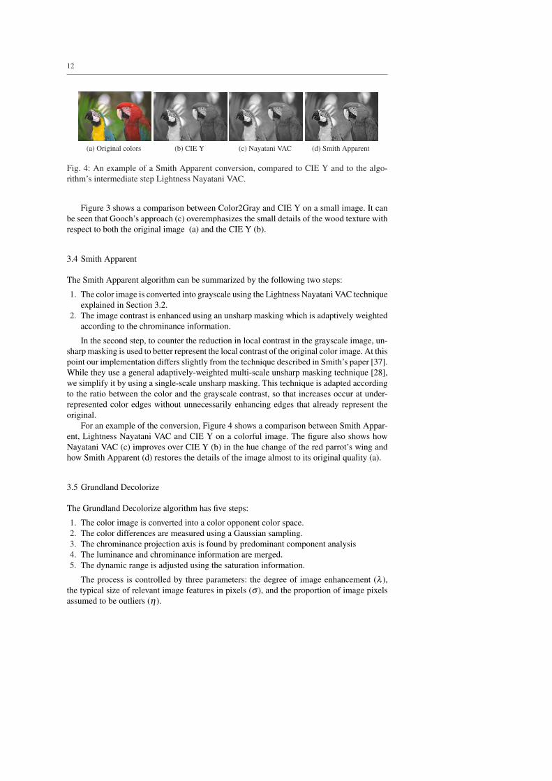
(a) Original colors (b) CIE Y (c) Nayatani VAC (d) Smith Apparent

Fig. 4: An example of a Smith Apparent conversion, compared to CIE Y and to the algo-rithm’s intermediate step Lightness Nayatani VAC.

Figure 3 shows a comparison between Color2Gray and CIE Y on a small image. It canbe seen that Gooch’s approach (c) overemphasizes the small details of the wood texture withrespect to both the original image (a) and the CIE Y (b).

3.4 Smith Apparent

The Smith Apparent algorithm can be summarized by the following two steps:

1. The color image is converted into grayscale using the Lightness Nayatani VAC techniqueexplained in Section 3.2.

2. The image contrast is enhanced using an unsharp masking which is adaptively weightedaccording to the chrominance information.

In the second step, to counter the reduction in local contrast in the grayscale image, un-sharp masking is used to better represent the local contrast of the original color image. At thispoint our implementation differs slightly from the technique described in Smith’s paper [37].While they use a general adaptively-weighted multi-scale unsharp masking technique [28],we simplify it by using a single-scale unsharp masking. This technique is adapted accordingto the ratio between the color and the grayscale contrast, so that increases occur at under-represented color edges without unnecessarily enhancing edges that already represent theoriginal.

For an example of the conversion, Figure 4 shows a comparison between Smith Appar-ent, Lightness Nayatani VAC and CIE Y on a colorful image. The figure also shows howNayatani VAC (c) improves over CIE Y (b) in the hue change of the red parrot’s wing andhow Smith Apparent (d) restores the details of the image almost to its original quality (a).

3.5 Grundland Decolorize

The Grundland Decolorize algorithm has five steps:

1. The color image is converted into a color opponent color space.2. The color differences are measured using a Gaussian sampling.3. The chrominance projection axis is found by predominant component analysis4. The luminance and chrominance information are merged.5. The dynamic range is adjusted using the saturation information.

The process is controlled by three parameters: the degree of image enhancement (λ ),the typical size of relevant image features in pixels (σ ), and the proportion of image pixelsassumed to be outliers (η).

13

(a) Original colors (b) CIE Y (c) Grundland Decolorize

Fig. 5: An example of a Grundland Decolorize conversion with a CIE Y reference.

The first step takes a linear RGB image (with values in the [0 ..1] range) and convertsit into their YPQ representation. The YPQ color space consists in a luminance channel Yand two color opponent channels: the yellow-blue P and the red-green Q channels. Theluminance channel Y is obtained with the NTSC Rec.601 formula, that is Yxy = 0.299Rxy +0.587Gxy +0.114Bxy, while P and Q with P = R+G

2 −B and Q = R−G. The perpendicular

chromatic axes support an easy calculation of hue H = 1π tan−1

(QP

)and saturation S =√

P2 +Q2.In the second step, to analyze the distribution of color contrasts between image features,

the color differences between pixels are considered. More specifically, the algorithm uses arandomized scheme: sampling by Gaussian pairing. Each image pixel is paired with a pixelchosen randomly according to a displacement vector from an isotropic bivariate Gaussiandistribution. The horizontal and vertical components of the displacement are each drawnfrom a univariate Gaussian distribution with 0 mean and 2

π σ variance.To find the color axis that represents the chromatic contrasts lost when the luminance

channel supplies the color to grayscale mapping, predominant component analysis is used.In the PQ chrominance plane, the predominant axis of chromatic contrast is determinedthrough a weighted sum of the oriented chromatic contrasts of the paired pixels. The weightsare determined by the contrast loss ratio2 and the ordering of the luminance. Unlike princi-pal component analysis which optimizes the variability of observations, predominant com-ponent analysis optimizes the differences between observations. The predominant chromaticaxis aims to capture the color contrast information that is lost in the luminance channel. Thedirection of the predominant chromatic axis maximizes the covariance between chromaticcontrasts and the weighted polarity of the luminance contrasts.

At this point (fourth step), the information on luminance and chrominance is combined.The predominant chromatic data values are obtained by projecting the chromatic data ontothe predominant chromatic axis. To appropriately scale the dynamic range of the predomi-nant chromatic channel the algorithm ignores the extreme values due to the level η of imagenoise. To detect outliers, a linear time selection algorithm is used to calculate the outlyingquantiles of the image data. The predominant chromatic channel is combined with the lumi-nance channel to produce the desired degree λ of contrast enhancement. At this intermediatestage of processing, the enhanced luminance is an image-dependent linear combination ofthe original color, which maps linear color gradients to linear luminance gradients.

2 The relative loss of contrast incurred when luminance differences are used to represent the RGB colordifferences.

14

The final step uses saturation to adjust the dynamic range of th enhanced luminancein order to exclude the effects of image noise and to expand its original dynamic rangeaccording to the desired degree λ of contrast enhancement. This is obtained by linearlyrescaling the enhanced luminance to fit the corrected dynamic range. Saturation is then usedto derive the bounds on the permitted distortion. To ensure that achromatic pixels retain theirluminance after conversion, the discrepancy between luminance and gray levels needs to besuitably bounded. The output gray levels are obtained by clipping the adjusted luminance toconform to the saturation dependent bounds.

The resulting transformation to gray levels is thus a continuous, piecewise linear map-ping of color and saturation values.

A comparison between Grundland Decolorize and CIE Y is shown in Figure 5. Thisimage is “difficult” to convert into grayscale because most of the salient features are quasi-isoluminant with respect to their surroundings. The figure shows how Grundland’s ap-proach (c) restores almost every feature of the color image (a) compared to a standardmethod such as CIE Y (b).

As already mentioned in Section 2.1.3, Grundland Decolorize is very sensitive to theissue of gamma compression. Figure 6 shows two examples of how an incorrect gammaassumption can decrease the quality of the results. A color image (a) has been linearizedand then converted correctly assuming linearity (b) and wrongly assuming sRGB gammacompression (c). To show the complementary case, an sRGB image (d) has been convertedwrongly assuming linearity (e) and correctly assuming its gamma compression (f). The lossof information is evident in the conversion which makes the wrong assumption: light ar-eas (c) or dark areas (e) lose most of the features because the saturation balancing interactsincorrectly with the outlier detection. Moreover, the predominant chromatic axis is perturbedand consequently the chromatic projection no longer retains its original meaning. Note forexample how the red hat and the pink skin (d), which should be mapped to similar grayintensities (f), are instead mapped to very different intensities (e).

4 Multi-Image Decolorize

In this section we propose a theoretically-motivated grayscale conversion that is ad-hoc forthe stereo and multi view stereo matching problem. Our conversion is a generalization ofthe Grundland Decolorize algorithm which simultaneously takes in input the whole set ofimages that need to be matched in order to be consistent with each other. In addition, twovariants of the conversion are also proposed:

1. The first variant performs the original version of the proposed algorithm and then appliesan unsharp masking filter in every image in order to enhance feature discriminability.

2. The second variant is similar to the first but uses a chromatic weighted unsharp maskingfilter instead of the classic one.

4.1 Requirements analysis

Our goal was to design a conversion that transforms the image set by preserving the consis-tency between the images that are to be matched, i.e., the same colors in different imagesneed to be mapped in the same gray values. In the meantime it optimizes the transformationby exploiting the color information. To make our analysis clearer we define the followingmatching requirements:

15

(a) Original image - lineargamma

(b) Correct assumption(gamma is linear)

(c) Wrong assumption (gammais sRGB)

(d) Original image - sRGBgamma

(e) Wrong assumption (gammais linear)

(f) Correct assumption(gamma is sRGB)

Fig. 6: Two examples of right and wrong gamma assumptions with Grundland Decolorize.

– Feature Discriminability: the method should preserve the image features discriminabil-ity to be matched as much as possible, even at the cost of decreased perceptual accuracyof the image3.

– Chrominance Awareness: the method should distinguish between isoluminant colors.– Global Mapping: while the algorithm can use spatial information to determine the map-

ping, the same color should be mapped to the same grayscale value for every pixel inthe image.

– Color Consistency: besides Global Mapping, the same color should also be mapped tothe same grayscale value in every image of the set to be matched.

– Grayscale Preservation: if a pixel in the color image is already achromatic it shouldmaintain the same gray level in the grayscale image.

– Low Complexity: if we consider the application of this algorithm in the context of multiview stereo matching, where a lot of images need to be processed, the computationalcomplexity gains importance.

In addition, the proposed algorithm should be unsupervised, i.e., it should not need usertuning to work properly.

4.2 Analysis of the state of the art

The Multi-Image Decolorize algorithm derives from a comprehensive analysis of the re-quirements described above. Our aim was to find the most suitable approach as a startingpoint for the development of our new technique.

3 We will talk about the interesting correlations between perceptual and matching results in Section 5.6.

16

Bala Spatial was considered inadequate because the spatial frequency based weightingof the importance of the H-K effect compared to the base lightness violates the Color Con-sistency and the Global Mapping requisites. As already mentioned, it was also susceptibleto problems in chroma and lightness misalignment.

Gooch Color2Gray violates, above all the low complexity requirement: its O(N4) com-putational complexity was really too much for our application, and even Mantiuk’s O(N2)improvement does not provide enough confidence in terms of to quality versus complex-ity. Moreover there are issues with the algorithm’s dependence on parameters that couldarbitrarily affect the grayscale mapping. This is good for artistic purposes but is not usefulwith for our objectives. Lastly, the gradient-based minimization process violates the ColorConsistency, Global Mapping and Grayscale Preservation requirements.

Queiroz Invertible was unsuitable for our needs since it is designed for “hiding” thecolor information in “invisible” parts of the grayscale image, which does not improve featurediscriminability in any way in terms of the standard conversions.

Rasche Monochromats has problems regarding the tradeoff between complexity andquality of the results because it quantizes colors. Moreover it applies an energy minimiza-tion process which violates Color Consistency, Global Mapping and Grayscale Preservationrequirements.

Neumann Adaptive is not appropriate for matching because image details and salientfeatures may be lost by unpredictable behavior in inconsistent regions of the gradient field.Another problem is that this approach is aimed too much towards human perceptual accu-racy.

Grundland Decolorize respects every requirement apart from Color Consistency, thuswe used this method as a starting point to develop our algorithm, extending it in order torespect such missing requirement.

The main problem with Alsam Sharpening and Smith Apparent is that, like Bala’s ap-proach, they violate our Color Consistency and Global Mapping requisites because of theirunsharp masking like filtering of the images. This is a problem with respect to our theoreticalrequirements. In fact, in this way colors are mapped inconsistently between different parts ofthe images depending on the surrounding neighborhoods. Despite this, in some preliminaryexperiments with our implementation of the Smith Apparent conversion with respect to theLightness Nayatani VAC we found that the advantages of unsharp masking did improve thematching results. This is not surprising, since it is well known that the unsharp masking filterenhances the fine details of the image. We thus also develop two variants of the Multi-ImageDecolorize by adding an unsharp masking filter to the converted image.

We would like to underline that the aforementioned requirements were sound in termsof improving of the matching task but, obviously, other ones can be defined to obtain per-formances improvement in the dense matching process.

4.3 The algorithm

Multi-Image Decolorize is an adaptation of the Grundland Decolorize algorithm which eval-uates the whole set of images in order to match them simultaneously. To achieve this, wemodified our implementation of Grundland’s algorithm in order to execute each of the fivesteps simultaneously for each image in the set. Initially, this seems equivalent to the follow-ing procedure:

1. Stitch together, side by side, all the images in the set in order to make one single bigimage.

17

2. Compute the Grundland Decolorize algorithm on the “stitched” image.3. Cut back the grayscale version of the original images.

Nevertheless, this simple implementation would not work correctly because, in the Gaussiansampling step, near the common borders of the images a pixel could be paired with a pixelnear the border of another image and the color differences estimation would be altered.

Instead in order to achieve the desired result, the implementation performs each step ofGrundland’s algorithm on each image in the set before performing the next step, using thesame accumulation variables for the predominant chromatic axis and for the quantiles ofnoise and saturation outliers. In this way, the matching requirements are fully applied to theset of images. In addition, the results benefit from the following transformation proprieties:

– Contrast Magnitude: the magnitude of grayscale contrasts visibly reflects the magnitudeof color contrasts.

– Contrast Polarity: the positive or negative polarity4 of gray level change in the grayscalecontrasts visibly corresponds to the polarity of luminance change in color contrasts.

– Dynamic Range: the dynamic range of gray levels in the grayscale image visibly matchesthe dynamic range of luminance values in the color image.

– Continuous mapping: the transformation from color to grayscale is a continuous func-tion. This reduces image artifacts, such as false contours in homogeneous image regions.

– Luminance ordering: when a sequence of pixels of increasing luminance in the colorimage share the same hue and saturation, they will have increasing gray levels in thegrayscale image. This reduces image artifacts, such as local reversals of edge gradients.

– Saturation ordering: when a sequence of pixels with the same luminance and hue in thecolor image has a monotonic sequence of saturation values, its sequence of gray levelsin the grayscale image will be a concatenation of at most two monotonic sequences.

– Hue ordering: when a sequence of pixels with the same luminance and saturation in thecolor image has a monotonic sequence of hue angles that lie on the same half of thecolor circle, its sequence of gray levels in the grayscale image will be a concatenationof at most two monotonic sequences.

In Fig. 7 we show how Multi-Image Decolorize is an improvement on Grundland Decol-orize when applied on a image pair. While Grundland’s approach gives better results whenconsidering the images separately, its results are inappropriate when the pair of images isconsidered together. For example see the “L–G–1” corner of the cube:

– In the “right” image (a), both Grundland (c) and the original version of Multi-ImageDecolorize (e) have to cope with the presence of the green “1” side, and they obtainsimilar results.

– In the “left” image (b), where the green “1” side does not appear, Grundland (d) distin-guishes the background of the “L” from the letter color better than the original versionof Multi-Image Decolorize (f).

– If the “left” and “right” images were matched, the vast majority of the algorithms wouldhave a greater probability of correctly matching the Multi-Image Decolorize pair (e)and (f) instead of the Grundland Decolorize pair (c) and (d).

This example is designed to emphasize the differences of the two approaches and toexplain the advantages of our adaptation, whereas in real life scenarios these situations occurin a softer way, at least in stereo matching. In multi view stereo matching, where more

4 That is the edge gradient.

18

(a) Original colors “right” (b) Original colors “left”

(c) Grundland Decolorize “right” (d) Grundland Decolorize “left”

(e) Multi-Image Decolorize “right” (f) Multi-Image Decolorize “left”

Fig. 7: Difference between Multi-Image Decolorize and Grundland Decolorize in a stereopair when chrominance changes significantly between the left and the right images.

19

Color Multi-Image Decolorize (MID) First variant (MID with USM) Second variant (MID with C-USM)

Fig. 8: Different conversions of a nearly isoluminant color test pattern.

images are involved, the benefits of a consistent mapping will be much more relevant evenin standard scenarios.

Like Grundland Decolorize, Multi-Image Decolorize is also sensitive to alterations inthe image gamma and, therefore, knowledge of the encoding of the starting image is essen-tial.

4.4 First variant: classic unsharp masking

The technique described in the previous section converts input images consistently and ap-propriately. However, because of dimensionality reduction, the contrast may be reduced. Tocounter the reduction, we increased the local contrast in the greyscale image using the ap-plication of an unsharp masking filter on the converted image. Unsharp masking (USM) isthe direct digital version of a well known darkroom analogic film processing technique [20]and is widely adopted in image processing [2] to improve the sharpness of a blurred image.

4.5 Second variant: chromatic weighted unsharp masking

The idea of using USM filtering to improve the results derives from the experimental per-formance of the Smith Apparent [37] technique, which is essentially a combination of theLightness Nayatani VAC conversion with an ad-hoc USM filter. They adopted a chromatic-based adaptively-weighted version of the USM filter, which we simply call chromatic un-sharp masking (C-USM), to counter the loss of chromatic contrast that derives from unac-counted hue differences. The technique is adapted according to the ratio between colourand greyscale contrast, so that increases occur at underrepresented color edges without un-necessarily enhancing edges that already represent the original. Thus this filter is able tobetter represent the local contrast of original colors. We used a single scale simplification ofC-USM, the same used in our implementation of the Smith Apparent method. The originalimplementation used in Smith’s paper is multi-scale [37].

The effect of the local chromatic contrast adjustment is illustrated in Figure 8 where anearly isoluminant color test pattern is converted into grayscale using the original version ofthe Multi-Image Decolorize, its first variant (MID with USM) and its second variant (MIDwith C-USM). The figure shows how the second variant gives different results comparedto classical unsharp masking because it provides more contrast only where it is low in theconversion with MID and high in the color image (such as, in the last squares of the bottom

20

line). Where the contrast is good enough C-USM has a limited effect, for example, betweenthe squares in the last two columns of the second and third rows.

5 Experimental Results

In this section we will describe and discuss the results of the experimental evaluation of thegrayscale conversions applied in the stereo matching context. We will show how the choiceof the color to gray conversion preprocessing influences the precision of the reconstructionof a Depth Map (DM in the following) from a single stereo pair.

After the introduction of the StereoMatcher framework used to produce the results (Sec-tion 5.1), we will describe the various experimental components (Section 5.2). Since thenumber of results generated is too large to be discussed in full detail, we will first show asmall subset in detail (Section 5.3). A comparison of Classic USM versus C-USM filtering(Section 5.4) is then presented and the general results are discussed (Section 5.5). Lastly wealso compare the observed results with a recent study [8] of the perceptual performances ofthe various grayscale conversions (Section 5.6).

5.1 The StereoMatcher framework

Stereo matching is one of the most active research areas in computer vision. While a largenumber of algorithms for stereo correspondence estimation have been developed, relativelylittle work focused on characterizing their performance until 2002, when Scharstein andSzeliski presented a taxonomy, a software platform called StereoMatcher and an evalua-tion [34] of dense two frame stereo methods. The proposed taxonomy was designed to as-sess the different components and design decisions made in individual stereo algorithms.The computation steps of the algorithms can be roughly aggregated as:

1. Matching cost computation2. Cost (support) aggregation3. Disparity computation / optimization4. Disparity refinement

We used StereoMatcher to assess the impact of color to gray conversions. StereoMatcheris closely tied to the taxonomy just presented and includes window-based algorithms, dif-fusion algorithms, as well as global optimization methods using dynamic programming,simulated annealing, and graph cuts. While many published methods include special fea-tures and post processing steps to improve the results, StereoMatcher implements the basicversions of these algorithms (which are the most common) in order to specifically assesstheir respective merits.

5.1.1 Color processing in the StereoMatcher framework

The color is treated in the first step, which involves the computation of the matching cost. InStereoMatcher, the matching cost computation is the squared or absolute difference in color/ intensity between corresponding pixels. To approximate the effect of a robust matchingscore [6,33], the matching score is truncated to a maximal value. When color images arecompared, the sum of the squared or the absolute intensity difference in each channel beforeapplying the clipping can be used. If a fractional disparity evaluation is being performed,

21

each scanline is first interpolated using either a linear or cubic interpolation filter [22]. It isalso possible to apply Birchfield and Tomasi’s sampling insensitive interval-based match-ing criterion [5], i.e., they take the minimum of the pixel matching score and the score at± 1

2 -step displacements, or 0 if there is a sign change in either interval. This criterion isapplied separately to each color channel to simplify the implementation. In the words ofthe authors, this is not physically plausible (the sub-pixel shift must be consistent acrosschannels). While this treatment has the advantage of using the color information, we beliveit is inappropriate for our purposes, because when a color image is given it blindly sumsthe absolute or the squared differences. Moreover, when the sampling insensitive matchingcriterion is used, it may introduces significant inconsistencies.

Instead, we separated the color treatment from the matching cost computation by build-ing a preprocessing tool to convert the original datasets and we used these resulting grayscaledatasets as inputs for the StereoMatcher. As can be seen in the results, our approach some-times provided an improvement compared to the results of the described color processing.

5.2 Description of the experiments

To thoroughly evaluate how the choice of different grayscale conversions affects the resultscomputed by the StereoMatcher algorithms we performed a large battery of tests. Thou-sands of error measures were computed, crossing different grayscale conversions with dif-ferent StereoMatcher algorithms and with different datasets. Here, we only report the mostrepresentative and significant results. To describe the experiments we will catalog their com-ponents as follows:

1. Datasets: we used different datasets with groundtruth, which are some of the standarddatasets used in the Computer Vision community.

2. StereoMatcher algorithmic combinations: we used six different standard algorithms toobtain the depth maps.

3. Classes of error measures: we used two different kinds of measures of the computeddepth maps errors.

4. Areas of interest of the error measure: we measured the errors in four different charac-terized parts of the depth maps.

5. Grayscale conversions: we used both the original color datasets and 11 different gray-scale conversions.

This classification, detailed in the next sections, facilitates a comparison of the advantagesand disadvantages of the grayscale conversions in terms of both the StereoMatcher algo-rithms and the peculiarities of the datasets.

5.2.1 The datasets

As just stated, the datasets employed in our experiments comes mainly from many subse-quent works of StereoMatcher authors [18,32], except one dataset, proposed by Nakamurain 1996 [23] and redistributed by them. These datasets are:

– The 1996 “tsukuba” dataset.– Three 2001 datasets: “sawtooth”, “venus” and “map”– Three 2005 datasets: “dolls”, “laundry” and “reindeer”.– Three 2006 datasets: “aloe” and “cloth” “plastic”.

22

The datasets selected from these are: the “aloe”, “cloth”, “laundry”, “dolls” and “map”. The“map” dataset was originally in grayscale and was used only to validate the requirement thatour conversion preserves the image quality when the colors were already achromatic.

We have no information on the gamma encoding of these datasets, however, using em-pirical measures of the image histogram distributions, we assume that only the datasets from2006 are gamma compressed. Comparisons between the results of the linear-assuming andthe sRGB-assuming versions of the Multi-Image Decolorize conversion seem to confirmthis hypothesis.

5.2.2 The StereoMatcher algorithmic combinations

The dense stereo matching process takes two rectified images of a three dimensional sceneand computes a disparity map, an image that represents the relative shift in scene featuresbetween the images. The magnitude of this shift is inversely proportional to the distancebetween the observer and the matched features. In the experiments, to obtain the computeddepth maps we used the following StereoMatcher algorithmic combinations:

– WTA: a Winner Take All disparity computation,– SA: a Simulated Annealing disparity computation,– GC: a Graph Cuts disparity computation.

The Winner Take All disparity computation algorithm simply picks the lowest matchingcost as the selected disparity at each pixel. The Simulated Annealing and the Graph Cutsdisparity computations are two iterative energy minimization algorithms that try to enhancethe smoothness term of the computed disparity maps. We refer to [19] for the Graph Cuts al-gorithm and [34] for all the used algorithm and other StereoMatcher implementations. Eachdisparity computation was paired with either Squared Differences (SD) matching cost com-putation and Absolute Differences (AD) matching cost computation. As already explainedin Section 5.1.1, the AD matching cost simply sums the absolute RGB differences betweentwo pixels, while SD sums the squared RGB differences. Both cost computations truncatethe sum to a maximal value in order to approximate the effect of a robust matching score. Forevery algorithm we use a fixed aggregation window (the spatial neighborhood considered inthe matching of a pixel) and no sub-pixel refinements of the disparities.

5.2.3 The classes of error measures

To evaluate the performance of the various grayscale conversions, we needed a quantitativeway to estimate the quality of the computed correspondences. A general approach to thisis to compute error statistics with respect to the groundtruth data. The current version ofStereoMatcher computes the following two quality measures based on known groundtruthdata:

– rms-error: the root-mean-squared error, measured in disparity units.– bad-pixels: the percentage of bad matching pixels.

5.2.4 The areas of interest of error measures

In addition to computing the statistics over the whole image, StereoMatcher also focuess onthree different kinds of regions. These regions are computed by preprocessing the referenceimage and the groundtruth disparity map to yield the following three binary segmentations:

23

– textureless regions: regions where the squared horizontal intensity gradient averagedover a square window of a given size is below a given threshold;

– occluded regions: regions that are occluded in the matching image, i.e., where the for-ward-mapped disparity lands at a location with a larger (nearer) disparity;

– depth discontinuity regions: pixels whose neighboring disparities differ by more than apredetermined gap, dilated by a window of predetermined width.

These regions were selected to support the analysis of matching results in typical problem-atic areas. We considered only the non-occluded (nonocc) regions since this kind of measureis the most significant one for our purposes. In fact, the other problematic areas, such as thetextureless and occluded parts, could produce results that are not reliable in evaluating howthe conversions could help the matching process.

5.2.5 The grayscale conversion

We executed the StereoMatcher algorithms and measured the various error measures for thefollowing versions of the datasets:

1. Original color version, because we obviously needed a starting point to understand ifthe tested conversions would give worse, equal or even better results than the standardcolor approach.

2. CIE Y was chosen as the representative of “standard” grayscale conversions.3. Sharp CIE Y, that is CIE Y followed by classic USM.4. Chromatic Sharp CIE Y, that is CIE Y followed by C-USM.5. Gooch Color2Gray, as the representative of the iterative energy minimization conver-

sions.6. Lightness Nayatani VAC as it is the starting point of Smith Apparent.7. Sharp Lightness Nayatani VAC, that is Lightness Nayatani VAC followed by classic

USM.8. Smith Apparent, that is Lightness Nayatani VAC followed by C-USM, as the represen-

tative of the optimizing conversions that use spatial information.9. Grundland Decolorize, as it is the starting point of our Multi-Image Decolorize tech-

nique.10. The original version of Multi-Image Decolorize.11. The first variant of Multi-Image Decolorize, that is Multi-Image Decolorize followed by

USM.12. The second variant of Multi-Image Decolorize, that is Multi-Image Decolorize followed

by C-USM.

We computed these conversions for the five datasets just mentioned which gave a final num-ber of 12×5 = 60 datasets. We thus ran StereoMatcher on 60 datasets using three algorithms(WTA, SA, GC) with two error measures (AD and SD) for a total of 360 tests. Due to thehigh number of tests done ,in the next section we detail a subset of the obtained resultsthat are representative of the entire data collected. General consideration are presented inSection 5.5.

5.3 StereoMatcher results

First, the full details of three StereoMatcher algorithmic combinations with seven versionsof the “laundry” dataset are shown. This dataset, whose original stereo pair can be seen in

24

Fig. 9: DM groundtruth for the “laundry” dataset

Table 1: Legend of histograms

Color Version

Original color versionCIE YSharp CIE YChromatic Sharp CIE YGooch Color2GrayLightness Nayatani VACSharp Lightness Nayatani VACSmith ApparentGrundland DecolorizeOriginal Multi-Image DecolorizeFirst variant of Multi-Image DecolorizeSecond variant of Multi-Image Decolorize

Figures 10(a) and 10(b) and whose true disparity map can be seen in Fig. 9, presents thetypical situation in which our approach gives results that are similar or better than the usualcolor processing. The versions of the dataset that we show are:

– The original color version, in Fig. 10– CIE Y, in Fig. 11,– Gooch Color2Gray, in Fig. 12,– Lightness Nayatani VAC, in Fig. 13,– Smith Apparent, in Fig. 14,– Grundland Decolorize, in Fig. 15,– the original version of Multi-Image Decolorize, in Fig. 16.

The error measures of the various versions of the datasets follow the color codes presentedin the legend in Table 1. USM and C-USM variants are also included in the legend but arenot shown here. However we will use them in Section 5.4 for comparison purposes.

Since the results of the Absolute Differences and the Squared Differences variants of thealgorithms used are really similar we only show the Squared Differences. More specifically,for every dataset version we show:

– the Reference Frame in subfigure (a),– the Match Frame in subfigure (b),

25

(a) Reference Frame (b) Match Frame (c) DM from WTA (d) DM from SA (e) DM from GC

Fig. 10: The “laundry” original dataset and three reconstructed DMs. DM groundtruth is inFigure 9.


Fig. 11: The “laundry” dataset with CIE Y preprocessing and three reconstructed DMs.


Fig. 12: The “laundry” dataset with Gooch Color2Gray preprocessing and three recon-structed DMs.

– the disparity map for WTA in subfigure (c),– the disparity map for SA in subfigure (d),– the disparity map for GC in subfigure (e).

In Fig. 17 the histograms of the error measures are reported:

– Fig. 17(a) compares the errors when WTA is used,– Fig. 17(b) compares the errors when SA is used,– Fig. 17(c) compares the errors when GC is used.

The same scale is used for each histogram.This dataset contains elements, such as the background, which are really difficult for the

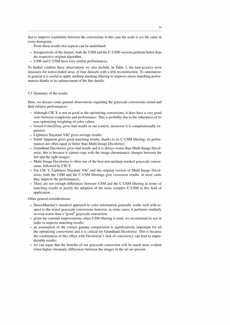
algorithms used. Our grayscale conversion is clearly the best one for this complex dataset,followed by Smith Apparent. When GC is used, Multi-Image Decolorize produces betterresults than color processing.

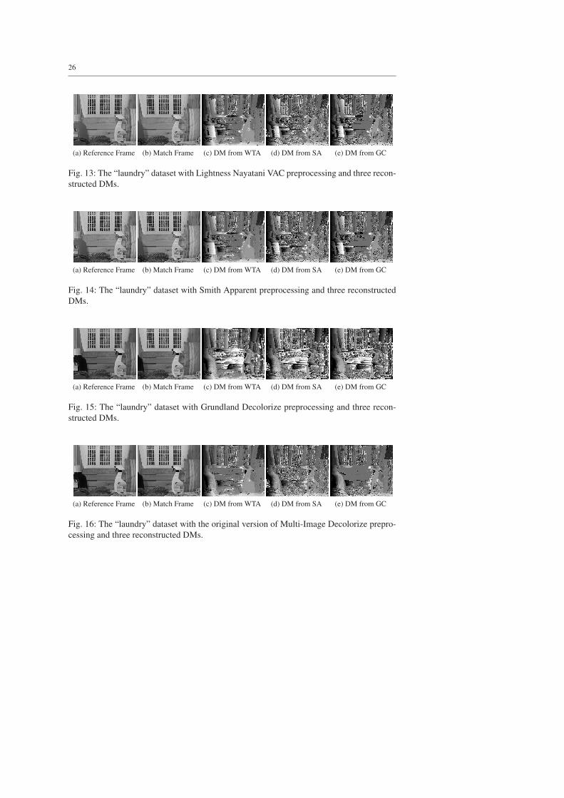
Another evident fact is the poor performance of Grundland Decolorize. This is becausein the Match Frame a big portion of the red bottle that was visible on the left of the Ref-erence Frame is no longer visible, heavily changing the global chrominance of the image.

26


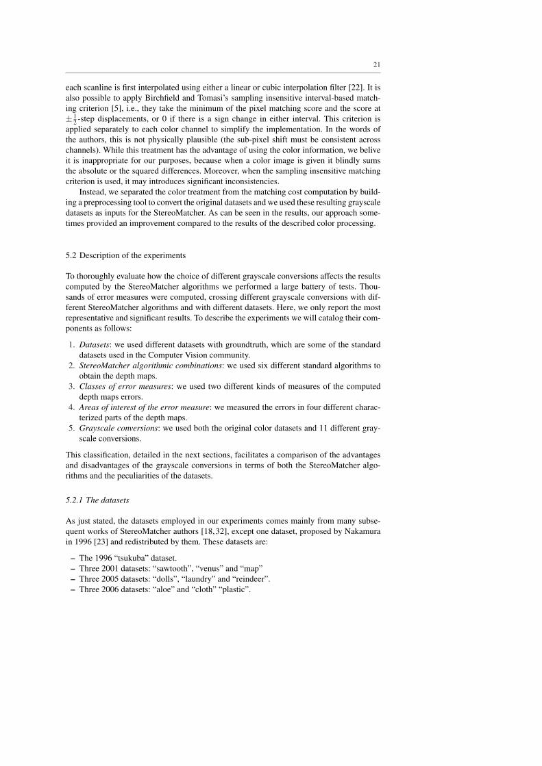
Fig. 13: The “laundry” dataset with Lightness Nayatani VAC preprocessing and three recon-structed DMs.


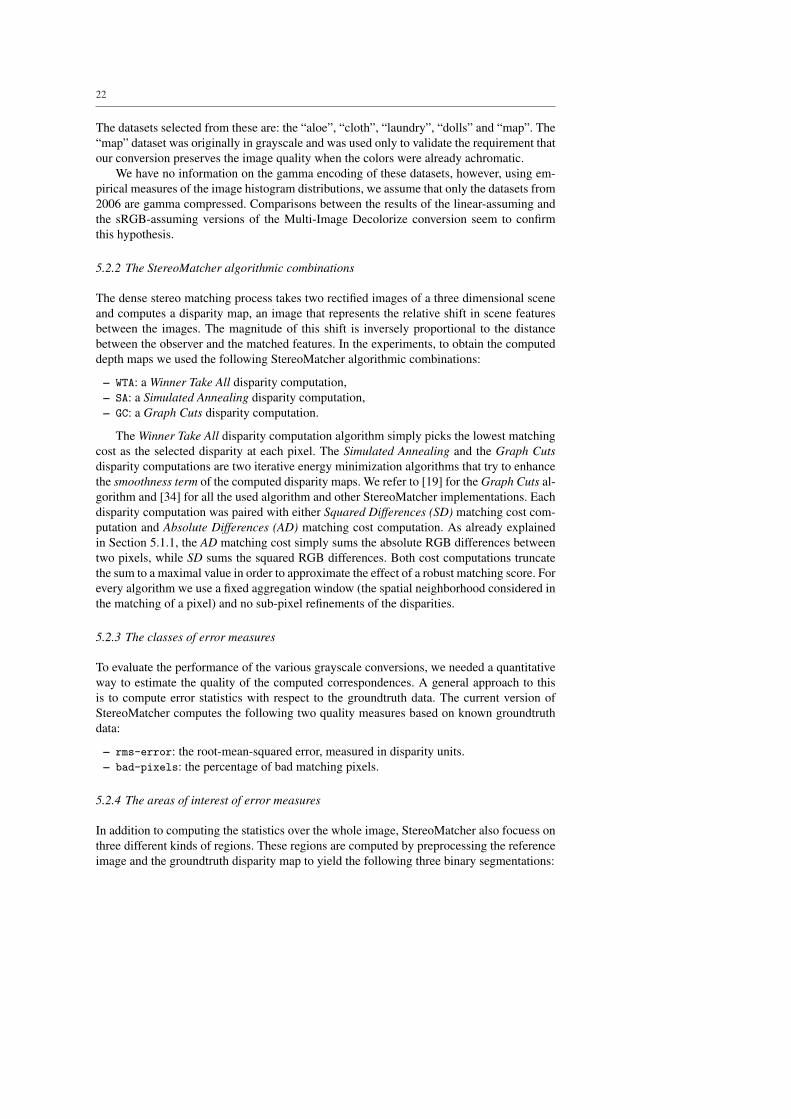
Fig. 14: The “laundry” dataset with Smith Apparent preprocessing and three reconstructedDMs.


Fig. 15: The “laundry” dataset with Grundland Decolorize preprocessing and three recon-structed DMs.


Fig. 16: The “laundry” dataset with the original version of Multi-Image Decolorize prepro-cessing and three reconstructed DMs.

27

(a) WTA (b) SA (c) GC

Fig. 17: rms-error of three StereoMatcher algorithms, in nonocc regions of the “laundry”dataset. The legend is in Table 1.

Table 2: bad-pixels of three StereoMatcher algorithms, in nonocc regions of four datasets,that compare the same versions of Fig. 17.

Original Lightness Originalcolor Gooch Nayatani Smith Grundland Multi-Image

version CIE Y Color2Gray VAC Apparent Decolorize Decolorizedataset algorithm

aloe GC 31.65% 21.99% 22.24% 22.51% 28.54% 26.84% 27.60%aloe SA 31.62% 27.17% 27.62% 28.16% 32.60% 31.37% 32.19%aloe WTA 10.06% 12.04% 12.21% 12.07% 9.90% 12.05% 11.64%

cloth GC 36.32% 27.03% 32.62% 28.35% 29.80% 33.95% 32.46%cloth SA 36.11% 35.85% 38.77% 37.01% 36.05% 39.04% 37.80%cloth WTA 10.82% 16.02% 16.95% 16.68% 12.09% 16.60% 15.31%

dolls GC 35.71% 33.14% 35.29% 34.04% 36.72% 38.72% 38.60%dolls SA 37.16% 40.45% 42.42% 41.13% 41.80% 45.68% 45.68%dolls WTA 20.02% 23.09% 23.96% 23.66% 20.80% 25.38% 25.17%

laundry GC 61.65% 56.64% 59.98% 58.50% 60.03% 87.74% 48.13%laundry SA 67.53% 71.39% 70.54% 72.07% 72.64% 88.87% 66.48%laundry WTA 43.22% 50.67% 54.19% 51.15% 47.06% 80.86% 45.65%

(a) The “aloe” dataset (b) The “cloth” dataset (c) The “laundry” dataset

Fig. 18: rms-error of WTA, in nonocc regions of three datasets, which compares the non-unsharped versions of CIE Y, Lightness Nayatani VAC and Multi-Image Decolorize withthe USM and C-USM versions. The legend is in Table 1.

28

Table 3: bad-pixels of WTA, in nonocc regions of four datasets, which compares the sameversions in Fig. 18

Sharp First SecondChromatic Lightness Lightness Original variant of variant of

Sharp Sharp Nayatani Nayatani Smith Multi-Image Multi-Image Multi-ImageCIE Y CIE Y CIE Y VAC VAC Apparent Decolorize Decolorize Decolorize

dataset

aloe 12.04% 9.86% 10.64% 12.07% 9.87% 9.90% 11.64% 9.66% 9.75%cloth 16.02% 11.66% 12.08% 16.68% 12.21% 12.09% 15.31% 11.47% 11.61%dolls 22.88% 20.30% 20.38% 23.03% 20.43% 20.51% 23.14% 20.42% 20.61%

laundry 50.67% 46.54% 46.72% 51.15% 47.37% 47.06% 45.65% 42.62% 42.86%

By analyzing the images separately, Grundland Decolorize finds a different chromatic pre-dominant axis of projection between the frames and thus assigns different grayscale valuesto the wood in the background. This causes the matching process in that region to fail, ashighlighted in Figures 15(c), 15(d) and 15(e).

Table 2 also includes the bad-pixels error measures for nonoccluded areas of the otherfour datasets with the WTA, SA and GC reconstruction. The table clearly shows that in generalthe best grayscale conversions are CIE Y, Smith Apparent and Multi-Image Decolorize, andoften the Original color version has a bigger error than one or more grayscale versions. CIEY often gives the best results when aggregative algorithms such as GC and SA are used.These measures confirm the poor performance of Grundland Decolorize.

5.4 Classic USM versus C-USM

Here we show how the choice of using either a classic USM or a C-USM after a grayscaleconversion affects the matching results. To do this we compare the results obtained for thefollowing grayscale conversions:

– CIE Y:– in its original version,– with classic USM postprocessing,– with C-USM postprocessing;

– Lightness Nayatani VAC:– in its original version,– with classic USM postprocessing,– with C-USM postprocessing (that corresponds to the Smith Apparent method);

– Multi-Image Decolorize:– in its original version,– with classic USM postprocessing,– with C-USM postprocessing;

on three different datasets, “aloe”, “cloth” and “laundry”. The USM and the C-USM imple-mentations are the same for each grayscale conversion. The reconstruction is performed byWTA and again we show the rms-error of non-occluded areas. In Figure 18 the histogramsof the error measures are reported; Figure 18(a) compares the errors for the “aloe” dataset,Figure 18(b) for the“cloth” dataset, and Figure 18(c) for the “laundry” dataset. Please note

29

that to improve readability between the conversions in this case the scale is not the same inevery histogram.

From these results two aspects can be underlined:

– Irrespectively of the dataset, both the USM and the C-USM versions perform better thanthe respective original algorithm.

– USM and C-USM have very similar performances.

To further confirm these observations we also include, in Table 3, the bad-pixels errormeasures for nonoccluded areas of four datasets with a WTA reconstruction. To summarize,in general it is useful to apply unsharp masking filtering to improve stereo matching perfor-mances thanks to its enhancement of the fine details.

5.5 Summary of the results

Here, we discuss some general observations regarding the grayscale conversions tested andtheir relative performances.

– Although CIE Y is not as good as the optimizing conversions, it does have a very goodratio between complexity and performance. This is probably due to the robustness of itsnon-optimizing weighting of color values.

– Gooch Color2Gray gives bad results in our context, moreover it is computationally ex-pensive;

– Lightness Nayatani VAC gives average results;– Smith Apparent gives good matching results, thanks to its C-USM filtering; its perfor-

mances are often equal or better than Multi-Image Decolorize;– Grundland Decolorize gives bad results and it is always worse than Multi-Image Decol-

orize, this is because it cannot cope with the image chrominance changes between theleft and the right images;

– Multi-Image Decolorize is often one of the best non unsharp-masked grayscale conver-sions, followed by CIE Y.

– For CIE Y, Lightness Nayatani VAC and the original version of Multi-Image Decol-orize, both the USM and the C-USM filterings give consistent results, in most casesthey improve the performances;

– There are not enough differences between USM and the C-USM filtering in terms ofmatching results to justify the adoption of the more complex C-USM in this field ofapplication.

Other general considerations:

– StereoMatcher’s standard approach to color information generally works well with re-spect to the tested grayscale conversions however, in some cases, it performs similarlyor even worse than a “good” grayscale conversion;

– given the constant improvements when USM filtering is used, we recommend its use inorder to improve matching results;

– an assumption of the correct gamma compression is significatively important for allthe optimizing conversions and it is critical for Grundland Decolorize. This is becausethe combination of this effect with Decolorize’s lack of consistency can lead to unpre-dictable results;

– we can argue that the benefits of our grayscale conversion will be much more evidentwhen higher chromatic differences between the images in the set are present.

30

5.6 Matching and perception

There are some interesting similarities between our results and an external study of theperceptual performances of many grayscale conversions that we used in this work.

From our knowledge, the study presented in Cadık et al. [8] is the first perceptual eval-uation of modern color to grayscale conversions. In this paper they presented the results oftwo subjective experiments in which a total of 24 color images were converted to grayscaleusing seven grayscale conversion algorithms and evaluated by 119 human subjects using apaired comparison paradigm. The grayscale conversions perceptually compared were: CIEY, Bala Spatial, Gooch Color2Gray, Rasche Monochromats, Grundland Decolorize, Neu-mann Adaptive and Smith Apparent. About 20000 human responses were used to evaluatethe accuracy and preference of the color to gray conversions. The final conclusions of thiswork have some similarites with our study. In both studies:

– Grundland Decolorize and consequently our Multi-Image Decolorize adaptation is oneof the best conversions.

– Smith Apparent is one of the best conversions.– CIE Y performs well notwithstanding its simplicity.

Obviously, the role of perception in machine vision algorithms is out of the scope of thiswork but it is an interesting point that stereo matching results are somewhat correlated tohuman perceptual preferences.

6 Conclusions

In this paper we examined the state of the art in color to gray conversions and discussedand evaluated how different grayscale conversions can affect the results of stereo matchingalgorithms. Starting with a qualitative analysis of the requirements needed to obtain a goodperformance in this field of application, we also adapted an existing conversion into theMulti-Image Decolorize, a method that seems to be more closely fitted to the matching task.Although the proposed algorithm did not always outperform some of the tested conversions,it also demonstrated good results in terms of the color processing of the StereoMatcher. Thisalgorithm can thus be seen as a first attempt to design an ad hoc grayscale conversion forfeature matching purposes.

From the analysis of the results we can also draw the following interesting considera-tions:

– The role of unsharp masking filtering is quite important and we found that by applyingan USM filter to grayscale images, the matching performances increase.

– A comparison between the classic USM and the C-USM demonstrates that standardUSM is powerful enough for matching purposes.

– In many cases, CIE-Y with classic USM can be a best compromise between efficiency,ease of implementation and quality of results.

6.1 Future Work

One of the most interesting future research possibilities to come out of this study concernsthe development of a grayscale conversion for image matching that does not rely on the

31

characteristics of the existing methods but computes the optimal conversion for matching,even at the cost of heavily-reduced quality from a perceptual viewpoint.

From an implementation/performance point of view such a conversion can be developedin a suitable way for GPU implementation in order to exploit the massive parallelization ofthe modern graphic hardware. An out-of-core mechanism could also be provided, in par-ticular for application in a multi-view matching context where many images need to beprocessed simultaneously.

Finally, a video conversion filter that works in real time and converts a video streammantaining the temporal consistence between the converted video frames would be interest-ing in certain video processing applications.

Acknowledgements This work was funded by the EU IST 3DCOFORM (7FP) project. We would like toacknowledge Martin Cadık, Daniel Scharstein, Richard Szeliski and Eastman Kodak Company for the imagesused in the paper and in the tests.

References

1. Alsam, A., Kolas, Ø.: Grey colour sharpening. In: Fourteenth Color Imaging Conference, pp. 263–267.Scottsdale, Arizona (2006)

2. Badamchizadeh, M.A., Aghagolzadeh, A.: Comparative study of unsharp masking methods for imageenhancement. International Conference on Image and Graphics 0, 27–30 (2004)

3. Bala, R., Eschbach, R.: Spatial color-to-grayscale transform preserving chrominance edge information.In: Color Imaging Conference, pp. 82–86 (2004)

4. Berns, R.S.: Billmeyer and Saltzman’s Principles of Color Technology, third edn. Wiley - Interscience(2000)

5. Birchfield, S., Tomasi, C.: Depth discontinuities by pixel-to-pixel stereo. International Journal of Com-puter Vision 35(3), 269–293 (1999)

6. Black, M., Rangarajan, A.: On the unification of line processes, outlier rejection, and robust statisticswith applications in early vision. International Journal of Computer Vision 19(1), 57–91 (1996)

7. Bleyer, M., Chambon, S., Poppe, U., Gelautz, M.: Evaluation of different methods for using colourinformation in global stereo matching approaches. In: The International Archives of the Photogrammetry,Remote Sensing and Spatial Information Sciences, vol. XXXVII, part B3a, pp. 415–422 (2008)

8. Cadık, M.: Perceptual evaluation of color-to-grayscale image conversions. Comput. Graph. Forum 27(7),1745–1754 (2008)

9. Chambon, S., Crouzil, A.: Color stereo matching using correlation measures. In: Complex SystemsIntelligence and Modern Technological Applications - CSIMTA 2004, Cherbourg, France, pp. 520–525.LUSAC (2004)

10. Fairchild, M., Pirrotta, E.: Predicting the lightness of chromatic object colors using CIELAB. ColorResearch & Application 16(6), 385–393 (1991)

11. Fairchild, M.D.: Color Appearance Models, second edn. Addison-Wesley (2005)12. Gonzalez, R.C., Woods, R.E.: Digital Image Processing, third edn. Prentice-Hall, Inc., Upper Saddle

River, NJ, USA (2006)13. Gooch, A.A., Olsen, S.C., Tumblin, J., Gooch, B.: Color2gray: salience-preserving color removal. ACM

Trans. Graph. 24(3), 634–639 (2005)14. Grundland, M., Dodgson, N.A.: The decolorize algorithm for contrast enhancing, color to grayscale

conversion. Tech. Rep. UCAM-CL-TR-649, University of Cambridge, Computer Laboratory (2005)15. Grundland, M., Dodgson, N.A.: Decolorize: Fast, contrast enhancing, color to grayscale conversion.

Pattern Recogn. 40(11), 2891–2896 (2007)16. Guild, J.: The colorimetric properties of the spectrum. Philosophical Transactions of the Royal Society

of London A230, 149–187 (1931)17. Hartley, R.I., Zisserman, A.: Multiple View Geometry in Computer Vision, second edn. Cambridge

University Press (2004)18. Hirschmuller, H., Scharstein, D.: Evaluation of cost functions for stereo matching. Computer Vision and

Pattern Recognition, IEEE Computer Society Conference on 0, 1–8 (2007)19. Kolmogorov, V., Zabih, R.: Computing visual correspondence with occlusions via graph cuts. Tech. rep.,

Ithaca, NY, USA (2001)

32

20. Langford, M.J.: Advanced photography: a grammar of techniques. Focal Press, Ltd. (1974)21. Mantiuk, R., Myszkowski, K., Seidel, H.P.: A perceptual framework for contrast processing of high

dynamic range images. ACM Transactions on Applied Perception 3(3), 286–308 (2006)22. Matthies, L., Kanade, T., Szeliski, R.: Kalman filter-based algorithms for estimating depth from image

sequences. International Journal of Computer Vision 3(3), 209–238 (1989)23. Nakamura, Y., Matsuura, T., Satoh, K., Ohta, Y.: Occlusion detectable stereo – occlusion patterns in

camera matrix. In: CVPR ’96: Proceedings of the 1996 Conference on Computer Vision and PatternRecognition (CVPR ’96), pp. 371–378. IEEE Computer Society, Washington, DC, USA (1996)

24. Nayatani, Y.: Simple estimation methods for the Helmholtz-Kohlrausch effect. Color Research & Appli-cation 22(6) (1997)

25. Nayatani, Y.: Relations between the two kinds of representation methods in the Helmholtz-Kohlrauscheffect. Color Research & Application 23(5) (1998)

26. Nayatani, Y., Sakai, H.: Confusion between observation and experiment in the Helmholtz-Kohlrauscheffect. Color Research & Application 33(3), 250–253 (2008)

27. Neumann, L., Cadık, M., Nemcsics, A.: An efficient perception-based adaptive color to gray transforma-tion. In: Proceedings of Computational Aesthetics 2007, pp. 73–80. Eurographics Association, Banff,Canada (2007)

28. Nowak, R., Baraniuk, R.: Adaptive weighted highpass filters using multiscale analysis. IEEE Transac-tions on Image Processing 7(7), 1068–1074 (1998)

29. de Queiroz, R.L., Braun, K.M.: Color to gray and back: color embedding into textured gray images.IEEE Transactions on Image Processing 15(6), 1464–1470 (2006)

30. Rasche, K., Geist, R., Westall, J.: Detail preserving reproduction of color images for monochromats anddichromats. IEEE Comput. Graph. Appl. 25(3), 22–30 (2005)

31. Reinhard, E., Khan, E.A., Akyz, A.O., Johnson, G.M.: Color Imaging: Fundamentals and Applications.A. K. Peters, Ltd., Natick, MA, USA (2008)

32. Scharstein, D., Pal, C.: Learning conditional random fields for stereo. Computer Vision and PatternRecognition, IEEE Computer Society Conference on 0, 1–8 (2007)

33. Scharstein, D., Szeliski, R.: Stereo matching with nonlinear diffusion. International Journal of ComputerVision 28(2), 155–174 (1998)

34. Scharstein, D., Szeliski, R.: A taxonomy and evaluation of dense two-frame stereo correspondence algo-rithms. Int. J. Comput. Vision 47(1-3), 7–42 (2002)

35. Sharma, G.: Digital Color Imaging Handbook. CRC Press, Inc., Boca Raton, FL, USA (2002)36. Shewchuk, J.R.: An introduction to the conjugate gradient method without the agonizing pain. Computer

Science Tech. Report pp. 94–125 (1994)37. Smith, K., Landes, P.E., Thollot, J., Myszkowski, K.: Apparent greyscale: A simple and fast conversion

to perceptually accurate images and video. Computer Graphics Forum (Proceedings of Eurographics2008) 27(2) (2008)

38. Tuytelaars, T., Mikolajczyk, K.: Local invariant feature detectors: a survey. Found. Trends Comput.Graph. Vis. 3(3), 177–280 (2008)

39. Vergauwen, M., Gool, L.V.: Web-based 3d reconstruction service. Mach. Vision Appl. 17(6), 411–426(2006)

40. Wright, W.D.: A re-determination of the trichromatic coefficients of the spectral colors. Transactions ofthe Optical Society 30, 141–164 (1928)

41. Wyszecki, G.: Correlate for lightness in terms of CIE chromaticity coordinates and luminous reflectance.Journal of the Optical Society of America 57(2), 254–254 (1967)

Color to gray conversions in the context of stereo matching

Documents

Transcript of Color to gray conversions in the context of stereo matching