Colloid Transport Project Project Advisors: Timothy R. Ginn, Professor, Department of Civil and...
22
Colloid Transport Project Project Advisors: Timothy R. Ginn, Professor, Department of Civil and Environmental Engineering, University of California Davis, Daniel M. Tartakovsky, Professor, Department of Mechanical and Aerospace Engineering University of Patricia J. Culligan, Professor, Department of Civil Engineering and Engineering Mechanics, Columbia
-
Upload
ferdinand-campbell -
Category
Documents
-
view
215 -
download
0
Transcript of Colloid Transport Project Project Advisors: Timothy R. Ginn, Professor, Department of Civil and...

Colloid Transport Project
Project Advisors:Timothy R. Ginn, Professor, Department of Civil and Environmental Engineering, University of California Davis,
Daniel M. Tartakovsky, Professor, Department of Mechanical and Aerospace Engineering University of
Patricia J. Culligan, Professor, Department of Civil Engineering and Engineering Mechanics, Columbia
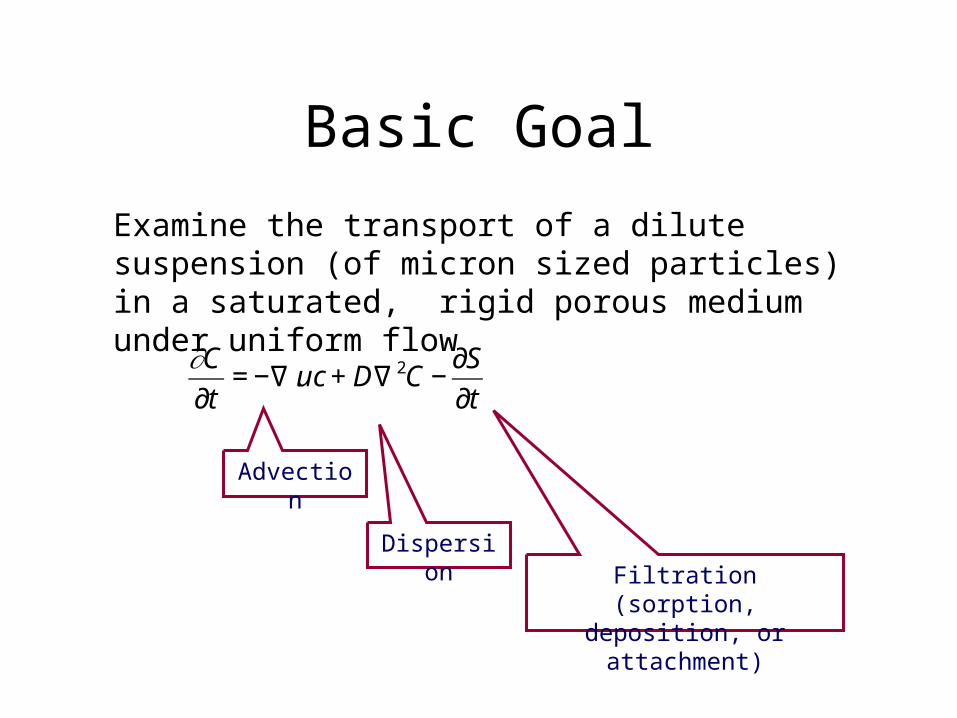
Basic Goal
Examine the transport of a dilute suspension (of micron sized particles) in a saturated, rigid porous medium under uniform flow
Advection
DispersionFiltration (sorption,
deposition, or attachment)
€
∂C
∂t= −∇.uc + D∇ 2C −
∂S
∂t

Challenge ∂S/∂t….
Classic mathematical models used to describe ∂S/∂t are inadequate in many cases - even in very simple systems

Problems Involving Particle Transport through Porous Media
• Water treatment system– Deep Bed Filtration (DBF)– Membrane-based filtration
• Transport of contaminants in aquifers– Colloidal particle transport
• Transport of microorganisms– Pathogen transport in groundwater– Bioremediation of aquifers
• Clinical settings– Blood cell filtration– Bacteria and viruses filtration

Particle Sizes10-2 10-310-410-510-610-710-810-910-10
(diameter, m)
1 Å 1 nm 1 m 1 mm 1 cm
Soils
Atoms,molecules
Microorganisms
Blood cells
Electronmicroscope
Light microscope Human eye
Depth-filtration range
Red blood cell
White blood cell
BacteriaViruses Protozoa
GravelSandSiltClay
Atoms MoleculesMacromolecules
Colloids Suspended particles

Particle Filtration through a Porous Medium
PorousMedium
Particle suspension injection at C0
Particle breakthrough
L
Time
Breakthrough concentration
C/Co < 1 C/Co Fraction of
particle mass is permanently removed by filtration

Idealized Description of Particle Filtration
• Clean-bed “Filtration Theory”GID ηηηη ++=0
€
αη
Single collector efficiency• Single “collector” represents a solid phase grain. A fraction η of the particles are brought to surface of the collector by the mechanisms of Brownian diffusion, Interception and/or Gravitational sedimentation. •A fraction α of the particles that reach the collector surface attach to the surface
• The single collector efficiency is then scaled up to a macroscopic filtration coefficient, which can be related to first-order attachment rate of the particles to the solid phase of the medium.
€
katt = λu
Filtration coefficient
First-order deposition rate
€
λ =3(1− n)
2dc
αη

Particle Filtration through a Porous Medium
PorousMedium
Particle suspension injection at C0
Particle breakthrough
L
€
C
Co
= exp(−λL)
Time
Breakthrough concentration
C/Co < 1 C/Co
€
∂S
∂t= kattC
€
katt = λu
katt (and αη) is assumed to be spatially constant and dependent upon particle-solid interaction energies (DLVO theory) and system physics

Motivation for Work
• Growing body of literature that indicates that katt decreases with transport distance - points to inadequacies in the filtration-theory
• Various solutions to fixing these inadequacies– More complex macroscopic models?– Modeling at the micro-scale?
• Examine solutions in context of a unique data set that has resolved particle concentrations in the interior of a porous medium in real time

Generation of Data Set• Translucent porous medium – glass beads saturated with water
• Laser induced fluorescent particles
– Micro-size Fluorescent Particles: Excitation wavelength 511-532nm, Emission wavelength 570-595nm.
– Laser : 6W Argon-ion Laser
• Digital image processing
– Captured images in real-time with CCD camera
– Image processing software

Particles
Acrylic particles with organic fluorescent dyes (fluorecein, rhodamine) embedded.
Specific gravity = 1.1
Particle size Range: 1-25 m,
d50=7m
Surface potential zeta-potential = -
109.97mV. Unlikely to attach to the glass bead surface due to the repulsive electrostatic force

Experimental Set Up
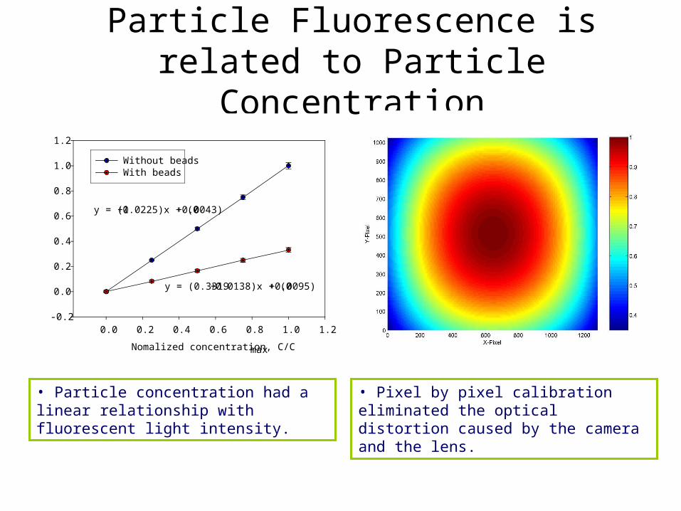
Particle Fluorescence is related to Particle Concentration
Nomalized concentration, C/Cmax
0.0 0.2 0.4 0.6 0.8 1.0 1.2
Normalized light intensity, I/I
max
-0.2
0.0
0.2
0.4
0.6
0.8
1.0
1.2
Without beadsWith beads
y = (1+0.0225)x + (0+0.0043)
y = (0.3319+0.0138)x + (0+0.0095)
Pixel (0 - 1024)
0 200 400 600 800 1000
Normalized intensity
0.2
0.4
0.6
0.8
1.0
1.2
• Particle concentration had a linear relationship with fluorescent light intensity.
• Pixel by pixel calibration eliminated the optical distortion caused by the camera and the lens.

Basic Experiment
Inject 10 Pore Volumes (PVs) of particle suspension at C = 50 mg/l
Follow with injection of 10 Pore Volumes (PVs) of non-particle suspension at C = 0 mg/l
Series of data for tests in similar porous media at difference values of uf

Data Available: Particle Breakthrough Curve at Column Base
Pore volumes
0 5 10 15 20
Normalized concentration, C/C
0
0.0
0.2
0.4
0.6
0.8
1.0
FastMediumSlow
€
∂C
∂t+
∂S
∂t= D
∂ 2C
∂z2− u
∂C
∂z
€
∂S
∂t=
∂Sirr
∂t+
∂Sr
∂t= kirr,attC + kr,attC + kr,detSr
Particle density versus time in fluid phase at base - C versus t at a fixed z
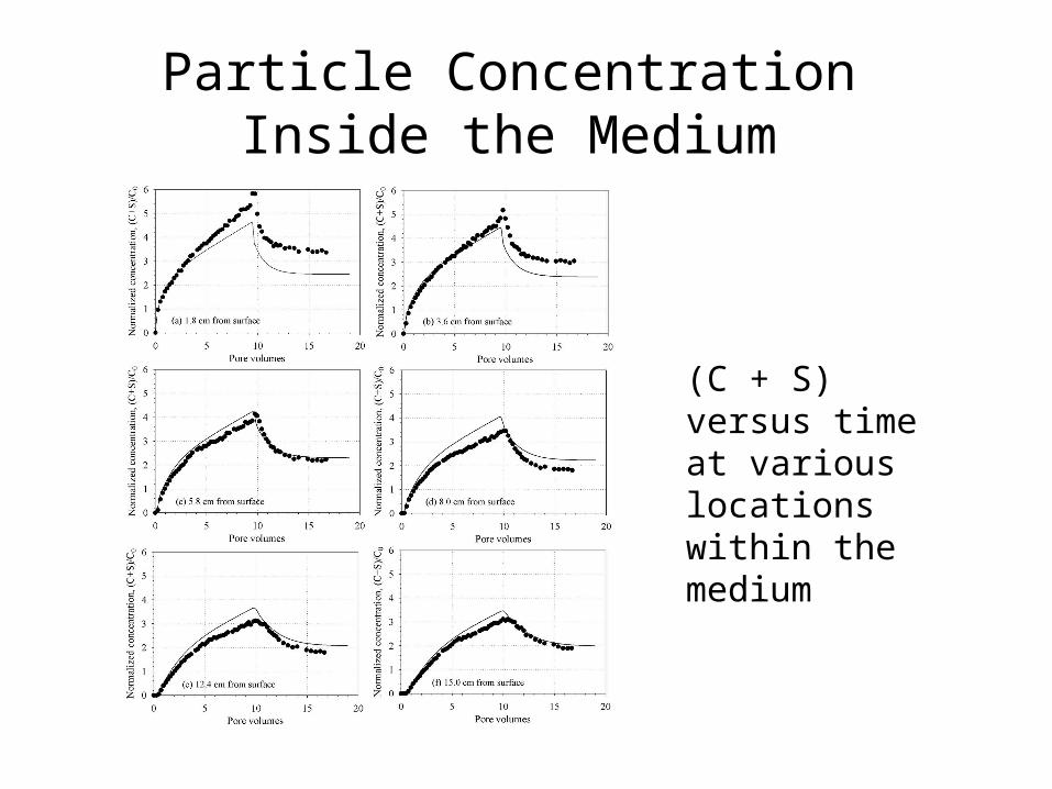
Particle Concentration Inside the Medium
(C + S) versus time at various locations within the medium

Microscopic Observations: Physical Insight
Flow direction
Particles are irreversibly attached at the solid-solid contact points (contact filtration) and at the top surface of the beads (surface filtration).
The particles are also reversibly attached at the surface of the beads and possibly at the contact points.
(a) to (c) Particle injection(d) to (e) Particle flushing

Contact Filtration• Particles moving near bead-
bead contact points were physically strained.
Bead-bead contacts
Bead-glass plate contacts
Flow direction

Surface Filtration
• Some of the particles that approached the surface of the beads became “irreversibly” attached.
Considering the highly negative zeta-potentials of the particles and beads, surface filtration must be “physical” - hypothesized that surface roughness held the particles against the drag force.
Flow direction

Project Tasks
Understand the data set
Model data using traditional filtration-theory Understand the inadequacies of this theory
Model data set using “more-complex” macroscopic balance equation
Can any of the coefficients in this balance equation be given a physical meaning?
Can micro-scale modeling techniques be applied and used to capture some of the observed behavior

What you will be given
Data sets for three experiments - each at different average fluid velocity
Experimental information - set-up plus parameters etc.
A library of background literature
Guidance, encouragement, hints (?)

What you will Deliver?
Project report = technical article that discusses the shortcomings of existing modeling approaches and explores avenues for improvements based on (a) macroscopic modeling approaches and (b) microscopic approaches