1

Collocations

(M&S Ch 5)

2

Introduction

• Collocations are characterized by limited

compositionality.

• Large overlap between the concepts of

collocations and terms, technical term and

terminological phrase.

• Collocations sometimes reflect interesting

attitudes (in English) towards different

types of substances: strong cigarettes, tea,

coffee versus powerful drug (e.g., heroin)

3

Definition (w.r.t Computational and

Statistical Literature)

• [A collocation is defined as] a sequence of

two or more consecutive words, that has

characteristics of a syntactic and semantic

unit, and whose exact and unambiguous

meaning or connotation cannot be derived

directly from the meaning or connotation of

its components. [Chouekra, 1988]

4

Other Definitions/Notions (w.r.t.

Linguistic Literature)

• Collocations are not necessarily adjacent

• Typical criteria for collocations: non-

compositionality, non-substitutability, non-

modifiability.

• Collocations cannot be translated into other

languages.

• Generalization to weaker cases (strong

association of words, but not necessarily

fixed occurrence.

5

Linguistic Subclasses of Collocations

• Light verbs: verbs with little semantic

content

• Verb particle constructions or Phrasal Verbs

• Proper Nouns/Names

• Terminological Expressions

6

Overview of the Collocation Detecting

Techniques Surveyed

• Selection of Collocations by Frequency

• Selection of Collocation based on Mean

and Variance of the distance between focal

word and collocating word.

• Hypothesis Testing

• Mutual Information

7

Frequency (Justeson & Katz, 1995)

1. Selecting the most frequently occurring

bigrams

2. Passing the results through a part-of-

speech filter

Simple method that works very well.

8

Mean and Variance (I)

(Smadja et al., 1993)

• Frequency-based search works well for fixed

phrases. However, many collocations consist

of two words in more flexible relationships.

• The method computes the mean and variance

of the offset (signed distance) between the

two words in the corpus.

• If the offsets are randomly distributed (i.e.,

no collocation), then the variance/sample

deviation will be high.

9

Mean and Variance (II)

• n = number of times two words collocate

• μ = sample mean

• di = the value of each sample

• Sample deviation:

n

i

i

n

μ)(ds

1

22

1

10

Example of flexible collocation

knocked on the door (3)

knocked at the door (3)

knocked on John’s door (5)

knocked on the metal front door (5)

μ = (3+3+5+5)/4 = 4

s = sqrt((3-4)2 + (3-4)2 + (5-4)2 + (5-4)2) / 3) = 1.15

If s is big => no collocation

If μ is not zero => flexible collocation

11

Hypothesis Testing: Overview

• High frequency and low variance can be accidental. We want to determine whether the co-occurrence is random or whether it occurs more often than chance.

• This is a classical problem in Statistics called Hypothesis Testing.

• We formulate a null hypothesis H0 (no association - only chance) and calculate the probability p that a collocation would occur if H0 were true, and then reject H0 if p is too low. Otherwise, retain H0 as possible.

12

Hypothesis Testing: The t-test

• The t-test looks at the mean and variance of a sample of measurements, where the null hypothesis is that the sample is drawn from a distribution with mean .

• The test looks at the difference between the observed and expected means, scaled by the variance of the data, and tells us how likely one is to get a sample of that mean and variance assuming that the sample is drawn from a normal distribution with mean .

• To apply the t-test to collocations, we think of the text corpus as a long sequence of N bigrams.

13

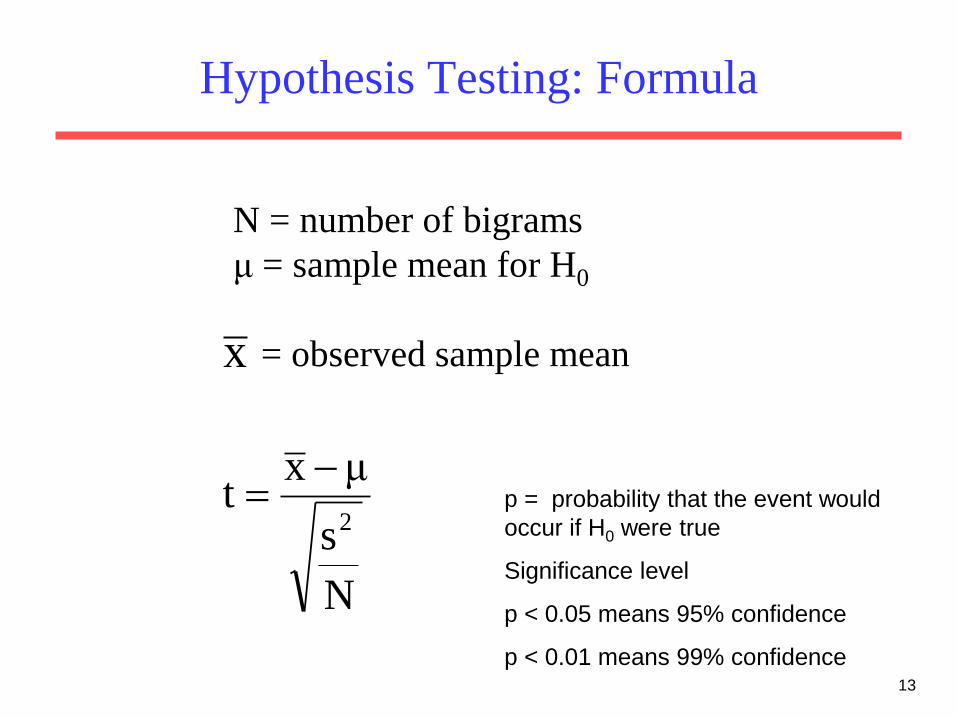
Hypothesis Testing: Formula

x

N = number of bigrams

μ = sample mean for H0

= observed sample mean

N

s

μxt

2

p = probability that the event would

occur if H0 were true

Significance level

p < 0.05 means 95% confidence

p < 0.01 means 99% confidence

14

Example

new companies – collocation or not?

w1 = new w1 ≠ new

w2 = companies O11 = 8 O12 = 4667

w2 ≠ companies O21 = 15820 O22 = 14287173

x

P(new) = (15820 + 8) / 14307668

P(companies) = (4667 + 8) / 14307668

H0: P(new companies) = P(new) * P(companies) = 0.0000003615 = μ

= 8 / 14307668 = 0.0000005591

s2 = p(1-p) ≈ p

576.2999932.0

14307668

910.00000055

0000003615.00000005591.0t

=> We cannot reject null hypothesis

15

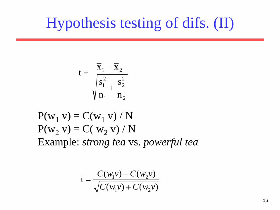
Hypothesis testing of differences (Church & Hanks, 1989)

• We may also want to find words whose co-

occurrence patterns best distinguish

between two words. This application can be

useful for lexicography.

• The t-test is extended to the comparison of

the means of two normal populations.

• Here, the null hypothesis is that the average

difference is 0.

16

Hypothesis testing of difs. (II)

2

2

2

1

2

1

21

n

s

n

x xt

s

P(w1 v) = C(w1 v) / N

P(w2 v) = C( w2 v) / N

Example: strong tea vs. powerful tea

)()(

)()(t

21

21

vwCvwC

vwCvwC

17

t-test for statistical significance of the

difference between two systems

System 1 System 2

scores 71,61,55,60,68,49,

42,72,76,55,64

42,55,75,45,54,51,

55,36,58,55,67

total 673 593

n 11 11

Mean 61.2 53.9

1081.6 1186.9

df 10 10

ix

^2^2 )x - (x sum s iij i

18

t-test for differences (continued)

• Pooled s2 = (1081.6 + 1186.9) / (10 + 10) = 113.4

• For rejecting the hypothesis that System 1 is better then

System 2 with a probability level of α = 0.05, the critical

value is t=1.725 (from statistics table)

• We cannot conclude the superiority of System 1 because

of the large variance in scores

60.1

11

113.4 2

53.961.2

n

2s 2

xxt

21

19

Chi-Square test (I): Method

• Use of the t-test has been criticized because it

assumes that probabilities are approximately

normally distributed (not true, generally).

• The Chi-Square test does not make this

assumption.

• The essence of the test is to compare observed

frequencies with frequencies expected for

independence. If the difference between observed

and expected frequencies is large, then we can

reject the null hypothesis of independence.

20

Chi-Square test (II): Formula

))()()((

)(

..............;.......;

)(

2221221221111211

2

211222112

222112

2111121111

2,1,

2

2

OOOOOOOO

OOOONX

EEE

NN

OO

N

OOE

E

EOX

ji ij

ijij

21

Chi-Square test (III): Applications

• One of the early uses of the Chi square test in

Statistical NLP was the identification of

translation pairs in aligned corpora (Church &

Gale, 1991).

• A more recent application is to use Chi square as

a metric for corpus similarity (Kilgariff and Rose,

1998)

• Nevertheless, the Chi-Square test should not be

used in small corpora.

22

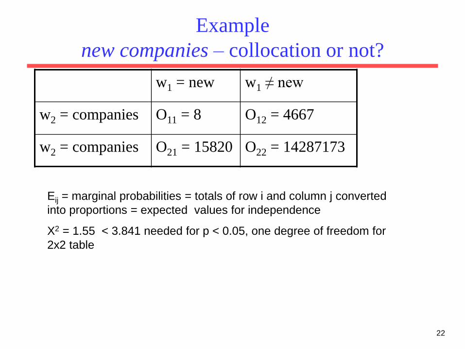
Example

new companies – collocation or not?

w1 = new w1 ≠ new

w2 = companies O11 = 8 O12 = 4667

w2 = companies O21 = 15820 O22 = 14287173

Eij = marginal probabilities = totals of row i and column j converted

into proportions = expected values for independence

X2 = 1.55 < 3.841 needed for p < 0.05, one degree of freedom for

2x2 table

23

Likelihood Ratios I: Within a single

corpus (Dunning, 1993)

• Likelihood ratios are more appropriate for sparse data than the Chi-Square test. In addition, they are easier to interpret than the Chi-Square statistic.

• In applying the likelihood ratio test to collocation discovery, we examine the following two alternative explanations for the occurrence frequency of a bigram w1 w2:

– The occurrence of w2 is independent of the previous occurrence of w1

– The occurrence of w2 is dependent of the previous occurrence of w1

24

Log likelihood

distrib. binomial - b and )1(),,( where

),,(log),,(log

),,(log),,(log

),;(),;(

),;(),;(

)(

)(loglog

);();();(;;;

)|()|(:

)|()|(:

211221112

1122112

211221112

1122112

2

1

21122211

1

1222

1

121

2

1221122

12121

knk xxxnkL

pcNccLpccL

pcNccLpccL

pcNccbpccb

pcNccbpccb

HL

HL

wwCcwCcwCccN

ccp

c

cp

N

cp

wwPppwwPH

pwwPwwPH

25

Likelihood Ratios II: Between two or more

corpora (Damerau, 1993)

• Ratios of relative frequencies between two

or more different corpora can be used to

discover collocations that are characteristic

of a corpus when compared to other

corpora.

• This approach is most useful for the

discovery of subject-specific collocations.

26

Mutual Information (I)

• An information-theoretic measure for

discovering collocations is pointwise

mutual information (Church et al., 89, 91)

• Pointwise Mutual Information is roughly a

measure of how much one word tells us

about the other.

• Pointwise mutual information does not

work well with sparse data.

27

Mutual Information (II)

)()(

),(log),(

)()(

),(log),(

)()(

),(log),(),(

yCxC

NyxCyxPMI

yPxP

yxPyxPMI

yPxP

yxPYXPyxMI

PMI = E (MI)

28

Example

PMI(new, companies) =

= log ((8 * 14307668) / (4675 * 15828)) = 1.546

PMI(house, commons) = 4.2

PMI(videocasette, recorder) = 15.94