COLLECTIVE MOVEMENT IN ROBOTIC SWARMS - …inaki/publications/THESIS2010_Navarro.pdf · COLLECTIVE...
179
Departamento de Autom´ atica, Ingenier´ ıaElectr´onica e Inform´ atica Industrial Escuela T´ ecnica Superior de Ingenieros Industriales COLLECTIVE MOVEMENT IN ROBOTIC SWARMS Autor I˜ naki Navarro Oiza Ingeniero de Telecomunicaci´ on Directores Fernando Mat´ ıa Espada Agust´ ın Jim´ enez Avello Doctor Ingeniero Industrial Doctor Ingeniero Industrial 2010
-
Upload
vuongnguyet -
Category
Documents
-
view
214 -
download
0
Transcript of COLLECTIVE MOVEMENT IN ROBOTIC SWARMS - …inaki/publications/THESIS2010_Navarro.pdf · COLLECTIVE...
Departamento de Automatica, Ingenierıa Electronicae Informatica Industrial
Escuela Tecnica Superior de Ingenieros Industriales
COLLECTIVE MOVEMENT
IN ROBOTIC SWARMS
Autor
Inaki Navarro OizaIngeniero de Telecomunicacion
Directores
Fernando Matıa Espada Agustın Jimenez AvelloDoctor Ingeniero Industrial Doctor Ingeniero Industrial
2010


Tribunal nombrado por el Mgfco. y Excmo. Sr. Rector de la Universidad Politecnicade Madrid, el dıa 28 de mayo de 2010.
Presidente: Dr. D. Ramon Galan Lopez
Vocal: Dr. D. Elio Tuci
Vocal: Dr. D. Miguel A. Salichs
Vocal: Dr. D. Jesus Manuel de la Cruz Garcıa
Secretario: Dr. D. Alvaro Gutierrez Martın
Suplente: Dr. D. Juan Gonzalez Gomez
Suplente: Dr. D. Jose Antonio Lopez Orozco
Realizando el acto de defensa y lectura de la Tesis el dıa de de 2010.
En la E.T.S. de Ingenieros Industriales.
CALIFICACION:
EL PRESIDENTE LOS VOCALES
EL SECRETARIO

Abstract
A novel framework for the control of collective movement of mobile robots ispresented and analysed. It allows a group of robots to move as a unique entityperforming the following functions: obstacle avoidance at group level, speed control,change of the inter-robot distance, splitting in sub-groups and rejoining groups into alarger one. Its basic controller is distributed among the robots, allowing them to movein the desired common direction and maintain a desired inter-robot distance.
The framework is composed of different modules that modify the behavior of thegroup allowing different functions. Most are based on consensus algorithms that allowthe robots to agree on different parameters, that consider which robot has more relevantinformation. New modules can be easily designed and incorporated to the frameworkin order to augment its capabilities. It can be easily implemented on any mobile robotcapable of measuring the relative positions of neighboring robots and communicatingwith them. It has been successfully tested using 8 real robots and in simulation with upto 40 robots, demonstrating experimentally the scalability with an increasing numberof robots.
The framework needs that robots have a common orientation reference, whichis calculated using a new developed distributed consensus method. This consensusalgorithm only needs that robots detect the relative positions of neighbors andcommunicate with them. Systematic experiments were carried out in simulation andwith real robots in order to test the method. Convergence has not been provedmathematically, but experimental results allows to trust on the use of the algorithm.Scalability with an increasing number of robots was tested successfully in simulationwith up to 49 robots. Experiments with real robots succeeded proving that the proposedmethod works in reality.
In order to analyze the performance of the framework, a set of metrics for collectivemovement is defined and and briefly discussed. Some of the metrics are useful just tocharacterize the algorithms while others can be used to compare their performance.

Resumen
En esta tesis se presenta y analiza un nuevo marco para el control del movimientocolectivo de robots moviles. Este marco permite que un grupo de robots se muevacomo una unica entidad, con las siguientes capacidades: evitacion de obstaculos a nivelde grupo, control de velocidad, posibilidad de cambio de la distancia entre robots,division en subgrupos de robots y unificacion de grupos en uno de mayor tamano. Elcontrolador principal se encuentra distribuido entre los robots, permitiendoles moverseen una direccion determinada comun y mantener una cierta distancia entre robots.
El marco esta compuesto por diferentes modulos que modifican el comportamientodel grupo mediante distintas funciones. La mayorıa de ellas se basan en algoritmosde consenso que permiten que los robots acuerden los valores de distintos parametros,teniendo en cuenta que robots aportan la informacion mas relevante. Las capacidadesdel marco pueden ampliarse facilmente mediante el diseno y la incorporacion de nuevosmodulos. El marco puede implementarse y utilizarse de forma sencilla en cualquiertipo de robot movil capaz de medir las posiciones relativas de sus robots vecinos y decomunicarse con ellos. Ha sido probado con exito con 8 robots reales y en simulacioncon hasta 40 robots, demostrando experimentalmente unas buenas propiedades deescalabilidad.
El marco requiere que los robots tengan una referencia comun de orientacion, la cualse calcula mediante un nuevo metodo de consenso distribuido que se ha desarrollado.Este algoritmo de consenso unicamente necesita que los robots detecten las posicionesrelativas de los robots proximos y que los robots puedan comunicarse entre sı. Se hanrealizado experimentos sistematicos tanto en simulacion como con robots reales paravalidar el metodo. La convergencia no ha sido probada matematicamente, pero losresultados experimentales invitan a confiar en el uso del algoritmo. Se han obtenidobuenos resultados de escalabilidad en simulacion con hasta 49 robots. Los experimentoscon robots reales muestran que el metodo propuesto funciona bien en la realidad.
Con el objetivo de analizar y evaluar el funcionamiento y comportamiento del marco,se definen y comentan brevemente una serie de metricas para el movimiento colectivo derobots. Algunas de ellas son utiles solamente para caracterizar los algoritmos mientrasque otras pueden utilizarse para comparar diferentes algoritmos.


A Cris y Luis


Agradecimientos
Hace ya mas de cinco anos, que sin saber muy que me esperaba, comence midoctorado. Desde entonces y hasta esta noche en que estoy escribiendo estas ultimaslineas, he pasado por etapas y momentos muy variados. A veces duros porque meencontraba perdido en el enfoque y avance de la tesis. Y otros buenos en los quenuevas ideas hacıan que los robots se comportaran incluso mejor de lo esperado. De loque estoy seguro es que he aprendido mucho. Y, por lo tanto, que ha merecido la pena.En estos anos de tesis, muchas personas que me han ayudado y aconsejado, tanto fueracomo dentro de la Universidad.
En primer lugar, agradecer a mis directores de tesis, Fernando Matıa y AgustınJimenez, por el apoyo y la ayuda recibida durante estos anos. Y por darme la libertadtanto para elegir el tema de tesis como para organizar mis tiempos y el desarrollode esta. Tambien mi agradecimiento a Ramon Galan, que aunque no haya sido midirector de tesis, ha estado siempre dispuesto a ayudarme y aconsejarme en todo lo quehe necesitado.
De gran ayuda tambien han sido Tere, Rosa y Carlos, tanto en los temasadministrativos y de papeleos, como en los animos para terminar la tesis. No meolvido tampoco de Angel, siempre dispuesto a ayudarme en todo lo tecnico que henecesitado, ya fuese en poner un cable para cargar los robots, como en ayudarme amanejar una camara. Gracias a los cuatro.
Muchas gracias a mis companeros y tambien amigos de departamento, con los quetantas conversaciones de cafeterıa, comidas y charlas hemos compartido. Gracias atodos: Jaime, Lupe, Paloma, Carlos, Ricardo, Alberto Brunete, Luis, Jose, Adolfo,Antonio, Alberto Valero y Xabi, por haber conseguido que ir cada dıa a la Universidadfuese divertido e interesante. Hemos aprendido y disfrutado juntos, y aun nos quedamucho.
De mi estancia en Lausanne tengo que dar las gracias a Alcherio por acogerme en sugrupo y ensenarme su metodologıa. Tambien a Jim por sus consejos sobre como avanzarde forma optima en una tesis doctoral y por desarrollar el sistema de posicionamientorelativo que me han permitido probar mis algoritmos en robots reales. A Thomas ledebo tambien el haber podido terminar la tesis utilizando los robots de una formasencilla gracias a sus proyectos Khepera III Toolbox y SwisTrack. Gracias tambien aXavier y a Nikolaus por su ayuda y consejos allı.
Mi agradecimiento a Lorena y Guillermo, que durante sus proyectos fin de carrerarealizaron experimentos, pruebas y codigo que han permitido probar los diferentesalgoritmos de la tesis.
Quiero agradecer a mi amigo Alvaro sus los consejos sobre el mundo investigador ydocente y tantos buenos y malos ratos compartidos aprendiendo con los robots. Muchasgracias tambien al resto de errebeceteros: Dani, Juanma y Jesus por su ayuda poniendoa punto las placas de posicionamiento relativo.
Ahora toca agradecer a mis amigos de fuera del ambito del doctorado. Tambienme habeis ayudado en la tesis, sobre todo con vuestros animos y apoyo. Me habrıagustado dedicaros a cada uno de vosotros unas palabritas, pero me vais a conceder que
xii
me lo salte, y cuando querais os lo cuento, aunque se que no hace falta. Corro el riesgode olvidarme de alguien. Gracias a mis companeros y amigos de teleco y alrededores:Rodrigo, Barri, Oscar, Rubio, Cristina, Ruben y Mata. Gracias a Rocıo. Gracias a miexcompanero de piso: Jesus. Gracias a mis excompaneras de piso: Valeria, Alessandra,Marıa, Paula, Fabienne y Renate. Gracias a mis lundianos originales: Valme, Zapata,Sonia, Javi, Marıa y Neli. Gracias a mis lundianos de la prorroga y sus alrededores:Alicia, Alex, Mario, Carmen, Francesca, Andrea, Fede, Jan, Vero y Anita. Gracias aTeresa. Gracias a mis amigos de toda la vida: Paloma, Jorge, Jaime, Pipe, Leyre yLucia. Y tambien, aunque sin saber como agrupar, gracias a Steffi, a Marta, a Alı, aTamara, a Marıa M.M y a Domingo.
Gracias tambien a Jose Gonzalez y a Nono, por interesarse siempre por mi tesis ypreguntar a menudo como iba.
Y ya casi por ultimo, quiero darles las gracias a mis dos abuelas por estar siempreatentas al desarrollo de mi tesis y por los animos que me han dado. Tambien, muchasgracias a mis primas, primos, tıas y tıos, por lo mismo, por preguntar, dar animos yaconsejar.
Por ultimo, muchas gracias a Cris y Luis, mis padres. Cris, estoy seguro de queLuis estarıa ahora leeyendo la tesis y pidiendome que le ensenase vıdeos de los robots.
Madrid, 5 de julio de 2010.

Contents
Abstract v
Resumen vii
Agradecimientos xi
Contents xiii
List of Figures xviii
List of Tables xxii
1 Introduction 11.1 Problem Statement . . . . . . . . . . . . . . . . . . . . . . . . . . . . . . 11.2 Main Objectives . . . . . . . . . . . . . . . . . . . . . . . . . . . . . . . 21.3 Document Layout . . . . . . . . . . . . . . . . . . . . . . . . . . . . . . . 3
I Background 5
2 Swarm Robotics 72.1 Introduction . . . . . . . . . . . . . . . . . . . . . . . . . . . . . . . . . . 72.2 Social Insect Motivation and Inspiration . . . . . . . . . . . . . . . . . . 82.3 Main Characteristics . . . . . . . . . . . . . . . . . . . . . . . . . . . . . 92.4 Swarm Robotics and Multi-robotic Systems . . . . . . . . . . . . . . . . 102.5 Experimental Platforms in Swarm Robotics . . . . . . . . . . . . . . . . 12
2.5.1 Robotic Platforms . . . . . . . . . . . . . . . . . . . . . . . . . . 122.5.2 Simulators . . . . . . . . . . . . . . . . . . . . . . . . . . . . . . . 13
2.6 Experimental Basic Behaviors and Tasks in Swarm Robotics . . . . . . . 162.6.1 Aggregation . . . . . . . . . . . . . . . . . . . . . . . . . . . . . . 162.6.2 Dispersion . . . . . . . . . . . . . . . . . . . . . . . . . . . . . . . 172.6.3 Pattern Formation . . . . . . . . . . . . . . . . . . . . . . . . . . 172.6.4 Collective Movement . . . . . . . . . . . . . . . . . . . . . . . . . 182.6.5 Task Allocation . . . . . . . . . . . . . . . . . . . . . . . . . . . . 182.6.6 Source Search . . . . . . . . . . . . . . . . . . . . . . . . . . . . . 192.6.7 Collective Transport of Objects . . . . . . . . . . . . . . . . . . . 19
xiv CONTENTS
2.6.8 Collective Mapping . . . . . . . . . . . . . . . . . . . . . . . . . . 192.7 Towards Real World Applications . . . . . . . . . . . . . . . . . . . . . . 202.8 Summary . . . . . . . . . . . . . . . . . . . . . . . . . . . . . . . . . . . 21
3 Collective Movement 233.1 Introduction . . . . . . . . . . . . . . . . . . . . . . . . . . . . . . . . . . 233.2 Collective Movement in Robotics . . . . . . . . . . . . . . . . . . . . . . 24
3.2.1 Classifications . . . . . . . . . . . . . . . . . . . . . . . . . . . . . 253.2.2 Functions of a Group of Robots Moving Collectively . . . . . . . 27
3.2.2.1 Aggregation . . . . . . . . . . . . . . . . . . . . . . . . 273.2.2.2 Moving to a Desired Place . . . . . . . . . . . . . . . . 273.2.2.3 Obstacle Avoidance . . . . . . . . . . . . . . . . . . . . 273.2.2.4 Splitting in Smaller Groups . . . . . . . . . . . . . . . . 283.2.2.5 Rejoining Groups . . . . . . . . . . . . . . . . . . . . . 283.2.2.6 Modifying the Inter-robot Distance . . . . . . . . . . . 293.2.2.7 External Shape Modification . . . . . . . . . . . . . . . 29
3.2.3 Review of Architectures . . . . . . . . . . . . . . . . . . . . . . . 303.2.3.1 First Work . . . . . . . . . . . . . . . . . . . . . . . . . 303.2.3.2 Initial Work in Formations . . . . . . . . . . . . . . . . 303.2.3.3 More Advanced Formations . . . . . . . . . . . . . . . . 313.2.3.4 Formations Based on Path Planning . . . . . . . . . . . 313.2.3.5 Other Formation Algorithms . . . . . . . . . . . . . . . 313.2.3.6 Reconfigurable Formations . . . . . . . . . . . . . . . . 323.2.3.7 Initialising Formations . . . . . . . . . . . . . . . . . . . 323.2.3.8 Formations Based on Common Coordinate System . . . 323.2.3.9 Scalable Lattice Formations . . . . . . . . . . . . . . . . 323.2.3.10 Graph Formalization of Formations . . . . . . . . . . . 333.2.3.11 Collective Movement Based on Consensus . . . . . . . . 333.2.3.12 Other Flocking Algorithms . . . . . . . . . . . . . . . . 343.2.3.13 Shape Control . . . . . . . . . . . . . . . . . . . . . . . 343.2.3.14 Splitting and Rejoining . . . . . . . . . . . . . . . . . . 343.2.3.15 Collective Movement Using Intelligent Control . . . . . 353.2.3.16 Collective Movement in 3 Dimensions . . . . . . . . . . 35
3.2.4 Applications . . . . . . . . . . . . . . . . . . . . . . . . . . . . . 353.3 Collective Movement in Animals . . . . . . . . . . . . . . . . . . . . . . 363.4 Other Collective Movements: Bicycle Critical Mass . . . . . . . . . . . . 373.5 Summary . . . . . . . . . . . . . . . . . . . . . . . . . . . . . . . . . . . 38
II Main 39
4 Metrics for Collective Movement of Robots 414.1 Introduction . . . . . . . . . . . . . . . . . . . . . . . . . . . . . . . . . . 414.2 Basic Definitions . . . . . . . . . . . . . . . . . . . . . . . . . . . . . . . 42

CONTENTS xv
4.3 Metrics . . . . . . . . . . . . . . . . . . . . . . . . . . . . . . . . . . . . 424.3.1 Shape . . . . . . . . . . . . . . . . . . . . . . . . . . . . . . . . . 43
4.3.1.1 Area . . . . . . . . . . . . . . . . . . . . . . . . . . . . . 444.3.1.2 Robot Density . . . . . . . . . . . . . . . . . . . . . . . 444.3.1.3 Isoperimetric Quotient . . . . . . . . . . . . . . . . . . 444.3.1.4 Mean Distance from the Boundary to the Center of the
Group . . . . . . . . . . . . . . . . . . . . . . . . . . . . 444.3.2 Movement . . . . . . . . . . . . . . . . . . . . . . . . . . . . . . . 45
4.3.2.1 Group Velocity . . . . . . . . . . . . . . . . . . . . . . . 454.3.2.2 Average Group Speed . . . . . . . . . . . . . . . . . . . 454.3.2.3 Length of the Trajectory . . . . . . . . . . . . . . . . . 45
4.3.3 Quality . . . . . . . . . . . . . . . . . . . . . . . . . . . . . . . . 454.3.3.1 Mean Position Error . . . . . . . . . . . . . . . . . . . . 464.3.3.2 Mean Distance Error . . . . . . . . . . . . . . . . . . . 464.3.3.3 Robot Density Error . . . . . . . . . . . . . . . . . . . . 474.3.3.4 Average Density Error . . . . . . . . . . . . . . . . . . . 474.3.3.5 Mean Orientation Error . . . . . . . . . . . . . . . . . . 474.3.3.6 Polarization . . . . . . . . . . . . . . . . . . . . . . . . 474.3.3.7 Percentage of Time in Formation . . . . . . . . . . . . . 484.3.3.8 Time to Be In Formation . . . . . . . . . . . . . . . . . 48
4.3.4 Efficiency and Cost . . . . . . . . . . . . . . . . . . . . . . . . . . 484.3.4.1 Path Length Ratio . . . . . . . . . . . . . . . . . . . . . 484.3.4.2 Single Robot Path Length Ratio . . . . . . . . . . . . . 494.3.4.3 Ratio Energy Consumption Distance Travelled . . . . . 49
4.3.5 Grouping . . . . . . . . . . . . . . . . . . . . . . . . . . . . . . . 494.3.5.1 Number of Subgroups . . . . . . . . . . . . . . . . . . . 504.3.5.2 Size of a Subgroup . . . . . . . . . . . . . . . . . . . . . 50
4.3.6 Success . . . . . . . . . . . . . . . . . . . . . . . . . . . . . . . . 504.3.6.1 Ratio of Lost Robots . . . . . . . . . . . . . . . . . . . 504.3.6.2 Ratio of Not Working Robots . . . . . . . . . . . . . . . 51
4.3.7 Security . . . . . . . . . . . . . . . . . . . . . . . . . . . . . . . . 514.3.7.1 Percentage of Time Group of Robots is Too Close to
Obstacles . . . . . . . . . . . . . . . . . . . . . . . . . . 514.3.8 Other . . . . . . . . . . . . . . . . . . . . . . . . . . . . . . . . . 51
4.3.8.1 Mean Number of Neighboring Robots . . . . . . . . . . 514.3.9 Higher Order Comparisons . . . . . . . . . . . . . . . . . . . . . 51
4.4 Conclusions . . . . . . . . . . . . . . . . . . . . . . . . . . . . . . . . . . 52
5 Distributed Orientation Agreement in a Group of Robots 535.1 Introduction . . . . . . . . . . . . . . . . . . . . . . . . . . . . . . . . . . 535.2 Consensus Problems . . . . . . . . . . . . . . . . . . . . . . . . . . . . . 545.3 Method . . . . . . . . . . . . . . . . . . . . . . . . . . . . . . . . . . . . 55
5.3.1 Consensus Algorithm A . . . . . . . . . . . . . . . . . . . . . . . 58
xvi CONTENTS
5.3.2 Consensus Algorithm B . . . . . . . . . . . . . . . . . . . . . . . 595.4 Experiments in Simulation . . . . . . . . . . . . . . . . . . . . . . . . . . 60
5.4.1 Set 1: CAA, Square Lattice Topology, α = 0.1, Random Turn . . 625.4.2 Set 2: CAA, Ring Topology, α = 0.1, Random Turn . . . . . . . 635.4.3 Set 3: CAA, Square Lattice Topology, α = 0.1, Alignment . . . . 635.4.4 Set 4: CAB, Square Lattice Topology, α = 0.1, Random Turn . . 645.4.5 Set 5: CAB, Square Lattice Topology, α = 0.01, Random Turn . 645.4.6 Set 6: CAB, Ring Topology, α = 0.1, Random Turn . . . . . . . 655.4.7 Set 7: CAB, Ring Topology, α = 0.3, Random Turn . . . . . . . 675.4.8 Set 8: CAB, Square Lattice Topology, α = 0.1, Alignment . . . . 675.4.9 Set 9: CAB, Square Lattice Topology, α = 0.1, Random Turn,
Clock Asynchronicity . . . . . . . . . . . . . . . . . . . . . . . . 685.5 Experiments with Real Robots . . . . . . . . . . . . . . . . . . . . . . . 68
5.5.1 Set 1: CAA, Square Lattice Topology, α = 0.1, Alignment . . . . 715.5.2 Set 2: CAB, Square Lattice Topology, α = 0.1, Alignment . . . . 72
5.6 Conclusions . . . . . . . . . . . . . . . . . . . . . . . . . . . . . . . . . . 745.7 Future Work . . . . . . . . . . . . . . . . . . . . . . . . . . . . . . . . . 75
6 Framework for Collective Movement of Mobile Robots 776.1 Introduction and Problem Statement . . . . . . . . . . . . . . . . . . . . 776.2 Robot Requirements for the Framework . . . . . . . . . . . . . . . . . . 78
6.2.1 Robots’ Mobility . . . . . . . . . . . . . . . . . . . . . . . . . . . 786.2.2 Robots’ Sensing . . . . . . . . . . . . . . . . . . . . . . . . . . . . 786.2.3 Inter-Robot Communications . . . . . . . . . . . . . . . . . . . . 78
6.3 The Framework . . . . . . . . . . . . . . . . . . . . . . . . . . . . . . . . 796.3.1 Common Orientation Agreement . . . . . . . . . . . . . . . . . . 806.3.2 Controllers . . . . . . . . . . . . . . . . . . . . . . . . . . . . . . 80
6.3.2.1 Basic Controller . . . . . . . . . . . . . . . . . . . . . . 806.3.2.2 Low Level Forward Movement Controller . . . . . . . . 846.3.2.3 Low Level Controller Forward-Backward Movement . . 84
6.3.3 Communication Systems . . . . . . . . . . . . . . . . . . . . . . . 856.3.4 Variable Consensus . . . . . . . . . . . . . . . . . . . . . . . . . . 856.3.5 Modules Overview . . . . . . . . . . . . . . . . . . . . . . . . . . 876.3.6 Individual Obstacle Avoidance Module . . . . . . . . . . . . . . . 886.3.7 Obstacle Avoidance Module . . . . . . . . . . . . . . . . . . . . . 886.3.8 Speed Control Module . . . . . . . . . . . . . . . . . . . . . . . . 916.3.9 Inter-Robot Distance Control Module . . . . . . . . . . . . . . . 926.3.10 Stop Control Module . . . . . . . . . . . . . . . . . . . . . . . . . 936.3.11 Splitting Control Module . . . . . . . . . . . . . . . . . . . . . . 946.3.12 Workings of the Framework . . . . . . . . . . . . . . . . . . . . . 95
6.4 Experiments in Simulation . . . . . . . . . . . . . . . . . . . . . . . . . . 966.4.1 Basic Collective Movement . . . . . . . . . . . . . . . . . . . . . 976.4.2 Collective Movement with Obstacles . . . . . . . . . . . . . . . . 99

CONTENTS xvii
6.4.3 Splitting in Sub-Groups and Rejoining . . . . . . . . . . . . . . . 1046.4.4 Inter-Robot Distance Control . . . . . . . . . . . . . . . . . . . . 110
6.5 Experiments with Real Robots . . . . . . . . . . . . . . . . . . . . . . . 1106.5.1 Basic Collective Movement . . . . . . . . . . . . . . . . . . . . . 1136.5.2 Collective Movement with Obstacles . . . . . . . . . . . . . . . . 1136.5.3 Splitting in Sub-Groups and Rejoining . . . . . . . . . . . . . . . 1206.5.4 Inter-Robot Distance Control . . . . . . . . . . . . . . . . . . . . 122
6.6 Related Work . . . . . . . . . . . . . . . . . . . . . . . . . . . . . . . . . 1226.7 Conclusions . . . . . . . . . . . . . . . . . . . . . . . . . . . . . . . . . . 1286.8 Future Work . . . . . . . . . . . . . . . . . . . . . . . . . . . . . . . . . 129
III Conclusions 131
7 Conclusions and Future Work 1337.1 Introduction . . . . . . . . . . . . . . . . . . . . . . . . . . . . . . . . . . 1337.2 Conclusions . . . . . . . . . . . . . . . . . . . . . . . . . . . . . . . . . . 1337.3 Future Work . . . . . . . . . . . . . . . . . . . . . . . . . . . . . . . . . 135
IV Appendix 137
A Experimental Platform 139A.1 The Khepera III Robot Platform . . . . . . . . . . . . . . . . . . . . . . 139
A.1.1 Khepera III Relative Positioning System . . . . . . . . . . . . . . 140A.2 Webots Robotic Simulator . . . . . . . . . . . . . . . . . . . . . . . . . . 140A.3 SwisTrack : Overhead Camera Tracking System . . . . . . . . . . . . . . 141
Bibliography 143

xviii CONTENTS
List of Figures
2.1 Taxonomy from Iocchi et al. (2001). For each level the correspondingtype of system is marked in dark grey for a swarm-robotic system. . . . 11
2.2 Images of the main robotic platforms used in swarm experiments. . . . . 15
3.1 Schematics showing different types of collective movements: (a) wingformation, (b) lattice (flocking or formation) and (c) flocking. . . . . . . 26
3.2 Schematic showing the aggregation mechanism of a group of robot anda later alignment of the individuals. . . . . . . . . . . . . . . . . . . . . 27
3.3 Schematic of a group of robots following a path together. . . . . . . . . 283.4 Schematic showing how a group of robots performs the obstacle avoid-
ance function. . . . . . . . . . . . . . . . . . . . . . . . . . . . . . . . . . 283.5 Schematic where a group of robots splits into two sub-group to overpass
an obstacle. . . . . . . . . . . . . . . . . . . . . . . . . . . . . . . . . . . 293.6 Schematic showing how two groups rejoin to become a unique group. . . 293.7 Schematic where a group of robots modifies its inter-robot distance in
order to pass through a corridor. . . . . . . . . . . . . . . . . . . . . . . 303.8 Schematic showing two external shape modifications: into a circle and
into a rectangle. . . . . . . . . . . . . . . . . . . . . . . . . . . . . . . . . 303.9 Flock of birds. . . . . . . . . . . . . . . . . . . . . . . . . . . . . . . . . 363.10 School of fishes. . . . . . . . . . . . . . . . . . . . . . . . . . . . . . . . . 373.11 Critical Mass event. . . . . . . . . . . . . . . . . . . . . . . . . . . . . . 38
4.1 The boundary of a group of robots is identified. . . . . . . . . . . . . . . 43
5.1 Angles involved in the calculation of θreference,i,j . . . . . . . . . . . . . 575.2 An initial condition in which CAA does not converge. . . . . . . . . . . 595.3 Communication topologies used in the experiments . . . . . . . . . . . . 615.4 Set 1: CAA, Square Lattice Topology, α = 0.1, Random Turn. . . . . . . 625.5 Set 2: CAA, Ring Topology, α = 0.1, Random Turn. . . . . . . . . . . . 635.6 Set 3: CAA, Square Lattice Topology, α = 0.1, Alignment. . . . . . . . . 645.7 Set 4: CAB, Square Lattice Topology, α = 0.1, Random Turn. . . . . . . 655.8 Set 5: CAB, Square Lattice Topology, α = 0.01, Random Turn. . . . . . 665.9 Set 6: CAB, Ring Topology, α = 0.1, Random Turn. . . . . . . . . . . . 665.10 Set 7: CAB, Ring Topology, α = 0.3, Random Turn. . . . . . . . . . . . 675.11 Set 8: CAB, Square Lattice Topology, α = 0.1, Alignment. . . . . . . . . 68

xx LIST OF FIGURES
5.12 Set 9: CAB, Square Lattice Topology, α = 0.1, Random Turn. . . . . . . 695.13 Communication topology of type square lattice used in the experiments
with real robots. . . . . . . . . . . . . . . . . . . . . . . . . . . . . . . . 695.14 Experimental setup of 8 robots placed in square lattice topology. . . . . 705.15 Set 1: CAA, Square Lattice topology, α = 0.1, Alignment, real robots. . 725.16 Set 2: CAB, Square Lattice topology, α = 0.1, Alignment, real robots. . 73
6.1 Schematic showing the ~vi,aggregation and ~vi,j for a set of six robots . . . . 826.2 Schematic depicts the basics of the determination of types of neighboring
robots . . . . . . . . . . . . . . . . . . . . . . . . . . . . . . . . . . . . . 836.3 Communication network from the point of view of robot r0. . . . . . . . 866.4 Schematics showing the propagation of θg with time, allowing obstacle
avoidance. . . . . . . . . . . . . . . . . . . . . . . . . . . . . . . . . . . . 906.5 Splitting into two sub-groups overview. . . . . . . . . . . . . . . . . . . . 956.6 Schematic showing the relations between the controllers, the different
modules and the common orientation agreement algorithm. Arrowsindicate the flow of information . . . . . . . . . . . . . . . . . . . . . . . 96
6.7 Relevant metrics and robots’ trajectories shown for a single experimentof Set1-40-sim tested in simulation. . . . . . . . . . . . . . . . . . . . . . 98
6.8 Trajectories of the robots during an experiment of Set3-40-sim whereobstacle avoidance and speed control are tested in simulation. The initialpositions of the robots are marked with a small circle, while the finalpositions are marked with a square. Visible obstacles are marked withred circles. . . . . . . . . . . . . . . . . . . . . . . . . . . . . . . . . . . . 102
6.9 Relevant metrics shown for an experiment of Set3-40-sim where obstacleavoidance and speed control are tested in simulation. . . . . . . . . . . . 103
6.10 Trajectories of the robots during an experiment of Set4-40-sim, wherethe rejoining function is tested in simulation. The initial positions of therobots, divided into groups (top left and top right), are marked with asmall circle. The final positions are marked with a square (bottom). . . 106
6.11 Relevant metrics shown for an experiment of Set4-40-sim, where therejoining function is tested in simulation. . . . . . . . . . . . . . . . . . 107
6.12 Trajectories of the robots during an experiment of Set5-40-sim, wherethe splitting function is tested in simulation. The initial positions ofthe robots are marked with a small circle (bottom). The final positions,where robots are split into two groups (top left and top right) are markedwith a square. . . . . . . . . . . . . . . . . . . . . . . . . . . . . . . . . . 108
6.13 Relevant metrics shown for an experiment of Set5-40-sim, where thesplitting function is tested in simulation. . . . . . . . . . . . . . . . . . . 109
6.14 Relevant metrics and robots’ trajectories shown for an experiment ofSet6-40-sim. The inter-robot distance control is tested in simulation. . . 112
6.15 Relevant metrics and robots’ trajectories shown for a single experimentof Set1-8-real tested with real robots. . . . . . . . . . . . . . . . . . . . . 115
LIST OF FIGURES xxi
6.16 Relevant metrics and robots’ trajectories shown for a single experimentof Set1b-8-real tested with real robots. . . . . . . . . . . . . . . . . . . . 116
6.17 Trajectories of the robots during an experiment of Set2-8-real whereobstacle avoidance and speed control are tested with real robots. Theinitial positions of the robots are marked with a small circle, while thefinal positions are marked with a square. . . . . . . . . . . . . . . . . . . 118
6.18 Relevant metrics shown for an experiment of Set2-8-real where obstacleavoidance and speed control are tested with real robots. . . . . . . . . . 119
6.19 Relevant metrics and robots’ trajectories shown for an experiment ofSet4-8-real, where the rejoining function is tested with real robots. . . . 121
6.20 Relevant metrics and robots’ trajectories shown for an experiment ofSet5-40-real, where the splitting function is tested with real robots. . . . 123
6.21 Relevant metrics and robots’ trajectories shown for an experiment ofSet6-8-real, where the inter-robot distance control is tested with realrobots. . . . . . . . . . . . . . . . . . . . . . . . . . . . . . . . . . . . . . 125
A.1 A Khepera III robot. . . . . . . . . . . . . . . . . . . . . . . . . . . . . . 140A.2 Khepera III Relative Positioning Board. . . . . . . . . . . . . . . . . . . 141A.3 A Webots window showing a Khepera III robot. . . . . . . . . . . . . . 142

xxii LIST OF FIGURES

List of Tables
2.1 Taxonomy axes and explanation from Dudek et al. (1996). . . . . . . . 10
2.2 Summary of the main robotic platforms used in swarm experiments. . . 14
6.1 Characteristics of experiments performed in Set1-8-sim and Set1-40-sim,in which basic collective movement is tested in simulation. . . . . . . . . 100
6.2 Relevant statistics of experiments performed in Set1-8-sim and Set1-40-sim, in which basic collective movement is tested in simulation. . . . . . 100
6.3 Characteristics of experiments performed in Set2-7-sim, Set2-40-sim,Set3-8-sim and Set3-40-sim, where obstacle avoidance and speed controlare tested in simulation. . . . . . . . . . . . . . . . . . . . . . . . . . . . 101
6.4 Relevant statistics of experiments performed in Set2-7-sim, Set2-40-sim,Set3-8-sim and Set3-40-sim, where obstacle avoidance and speed controlare tested in simulation. . . . . . . . . . . . . . . . . . . . . . . . . . . . 104
6.5 Characteristics of experiments performed in Set4-8-sim, Set4-40-sim,Set5-8-sim and Set5-40-sim, where the rejoining and splitting capabilitiesof the framework are tested in simulation. . . . . . . . . . . . . . . . . . 105
6.6 Relevant statistics of experiments performed in Set4-8-sim, Set4-40-sim,Set5-8-sim and Set5-40-sim, where the rejoining and splitting capabilitiesof the framework are tested in simulation. . . . . . . . . . . . . . . . . . 111
6.7 Characteristics of experiments carried out in Set6-8-sim and Set6-40-simwhere the inter-robot distance control is tested in simulation. . . . . . . 111
6.8 Relevant statistics for the experiments performed in Set6-8-sim and Set6-40-sim where the inter-robot distance control is tested in simulation. . . 114
6.9 Characteristics of experiments performed in Set1-8-real and Set1b-8-real,in which basic collective movement is tested with real robots. . . . . . . 114
6.10 Relevant statistics of experiments performed in Set1-8-real and Set1b-8-real, in which basic collective movement is tested with real robots. . . . 117
6.11 Characteristics of experiments performed in Set2-7-real and Set3-8-real,where the obstacle avoidance and speed control capabilities are testedwith real robots. (*) The arena used in Set3-8-real is bounded but onlyone of the limiting walls is inside the camera view, so just the visiblepart of the arena is used when analysing the experiments. Experimentswere stopped when one of the robots exited the visible area. . . . . . . . 117

xxiv LIST OF TABLES
6.12 Relevant statistics of experiments performed in Set2-7-real and Set3-8-real, where obstacle avoidance and speed control are tested with realrobots. . . . . . . . . . . . . . . . . . . . . . . . . . . . . . . . . . . . . . 119
6.13 Characteristics of experiments performed in Set4-8-real, and Set5-8-real,where the rejoining and splitting capabilities of the framework are testedwith real robots. . . . . . . . . . . . . . . . . . . . . . . . . . . . . . . . 120
6.14 Relevant statistics of experiments performed in Set4-8-real and Set5-8-real, where rejoining and splitting capabilities of the framework aretested with real robots. . . . . . . . . . . . . . . . . . . . . . . . . . . . 122
6.15 Characteristics of experiments carried out in Set6-8-real where the inter-robot distance control is tested with real robots. . . . . . . . . . . . . . 124
6.16 Relevant statistics for the experiments carried out in Set6-8-real wherethe inter-robot distance control is tested with real robots. . . . . . . . . 124

Chapter 1
Introduction
All men seek one goal: success or happiness. First have a definite clear,practical ideal - a goal, an objective. Second have the necessary means toachieve your ends - wisdom, money, materials, and methods. Third, adjustall your means to that end.
Aristotle
1.1 Problem Statement
Collective movement of mobile robots has been recognized as one of the basic andfundamental problems in multi-robot systems. There are many applications in which amulti-robot approach can be an advantage compared to the one based on single robots.Collective movement then represents a starting point for more complex tasks such ascollective mapping, search tasks, teleoperation by a single operator of a group of robots,etc.
Collective movement of robots is the problem of how to make mobile robots movetogether as a group, behaving as a single entity. It can be classified into flocking andformations of robots. In flocking, robots move as a group but the shape and relativepositions between the robots are not fixed, allowing robots to move within the group.On the other hand, a robot formation can be defined as a group of robots that is able tomaintain pre-determined positions and orientations between its members at the sametime that it moves as a whole.
Many different solutions have been implemented to the collective movementproblem. Some of them imply the existence of a leader that moves while is followed byone or more robots that may also act as leaders for other robots. The main disadvantageof this type of architecture is that it does not scale well with an increasing number ofrobots since the position error propagates cumulatively from leader to follower. In theother type of solutions no leaders are designated and robots react to the positions oftheir neighboring robots, and moving in an emergent direction. These last solutionsusually need global information according to the desired direction movement, whichmakes them not scalable. Some of the solutions allow obstacle avoidance at grouplevel, and some even allow to split the group into sub-groups to overcome obstacles
2 Chapter 1. Introduction
and then rejoin. There are formation solutions that allow the group of robots tochange its global shape. It is difficult to find a solution that is general enough tocontemplate the desirable properties and functions of: scalability with the number ofrobots, obstacle avoidance at group level, possibility of splitting the group in severalsub-groups, agreement among the robots on the direction of movement, etc. Thesolution we propose in this Thesis exploits a distributed and scalable approach thataims to be general enough to allow the implementation of these desirable properties.
1.2 Main Objectives
The main objective of this Thesis is the study of collective movement, together withthe development of a general framework for collective movement of mobile autonomousrobots. The proposed collective movement framework must be scalable with increasingnumber of robots, so local sensing and communications and a decentralized controllerare necessary. It must work without the use of any global information, so in principlerobots might know only the relative positions of nearby robots.
The framework should ideally be able to perform the following functions:
• Agreement on the direction of movement. Individuals should agree on thedirection the group takes. This direction can be given by an external entity, suchas a human teleoperator of the whole group, or can be the result of consensuswithin the group of robots.
• Obstacle avoidance at group level. The group of robots must be able toavoid obstacles and overcome them when necessary.
• Splitting. The group of robots might decide to split into sub-groups of robots.The reason could be to overcome an obstacle but also to explore an area in smallergroups.
• Rejoining. Different sub-groups can decide eventually to rejoin into a commonsingle group.
• Shape modification. Ideally the group of robots should be able to modify itsexternal shape to any desired one. Another possibility is that the group of robotsjust accommodate its shape to the environment without an intrinsic knowledgeof it.
It might also be as general and expandable as possible, allowing to include newfeatures and functions and to be modified in order to be used for different purposesand applications. The framework should be tested both in simulation and using a realrobotic platform.
In addition, it is necessary to have a set of metrics to evaluate the performanceof collective movement of mobile robots. The set of measurements used in roboticexperiments in order to define its performance must be identified and motivated whenreporting results. But the multi-robot research community working on collective

1.3. Document Layout 3
movement do not share a common set of metrics, and usually similar but not comparablemetrics are used. So it is necessary to define a set of metrics as complete as possible.
1.3 Document Layout
This Thesis is organized in three main parts. In Part I, the basic concepts thathelp to put the developed work into context are introduced. Chapter 2 introducesSwarm Robotics, relating it with other multi-robotic systems and stating its promisingapplications. A review of collective movement strategies and architectures in mobilerobotics, but as well in other systems composed of animals or people is developed inChapter 3.
In Part II a framework for collective movement of robots is developed and described,together with a set of metrics to measure it and applications that show its usefulness.The set of metrics is presented in Chapter 4 in order to measure and compare thedifferent collective movement algorithms. In Chapter 5 an algorithm for consensus ona reference heading among the robots is described and analysed. Chapter 6 describes,develops and analyses a framework for collective movement of mobile robots by meansof distributed controllers and consensus algorithms. It makes use of the algorithmpresented in Chapter 5.
Part III is dedicated to conclusions and future work. Chapter 7 discusses the mainaspects and contributions of this Thesis and suggests future lines of research.+
Lastly, Appendix A describes the experimental platform used in the experimentsthat were carried out in order to test and develop the proposed algorithms.

4 Chapter 1. Introduction

Part I
Background


Chapter 2
Swarm Robotics
E pluribus unum. (Out of many one).
Motto of the United States of America - It originally comes fromMoretum, a poem attributed to Virgil but of unknown author.
2.1 Introduction
Swarm Robotics is the study of how to coordinate large groups of relatively simplerobots through the use of local rules. It takes its inspiration from societies of insects,that can perform tasks that are beyond the capabilities of the individuals. Beni (2005)describes these kind of robots’ coordination as follows:
The group of robots is not just a group. It has some special characteristics,which are found in swarms of insects, i.e., decentralized control, lack ofsynchronization, simple and (quasi) identical members.
Swarm-robotic architectures intend to posses certain advantageous properties suchas robustness, flexibility and scalability, which are desirable in the developed algorithmsdescribed in this Thesis. This chapter summarizes the research performed during thelast years in this field of multi-robotic systems. The aim is to give a glimpse of SwarmRobotics and its applications. In Section 2.2 the motivation and inspiration of SwarmRobotics taken from social insects is explained. Section 2.3 continues addressing themain characteristics and possible disadvantages of Swarm Robotics. The relationshipof Swarm Robotics with multi-robotic systems in general is stated in Section 2.4.Different robotic platforms and simulators suitable for swarm-robotic experimentationare described in Section 2.5. Section 2.6 surveys the different results in solving tasksand performing basic behaviors using a swarm-robotic approach. Present and futurereal applications are depicted in Section 2.7. Lastly, in Section 2.8 the main ideas ofthis chapter are summarized.

8 Chapter 2. Swarm Robotics
2.2 Social Insect Motivation and Inspiration
The collective behaviors of social insects, such as the honey-bee’s dance, the wasp’snest-building, the construction of the termite mound or the trail following of ants,were considered for a long time strange and mysterious aspects of biology. Howcould these simple creatures solve such extraordinary and complex tasks? Duringthe 1960’s some researches pointed out that the complex behaviors of social insectswere based in the cognitive and representation capabilities of the individuals (Thorpe,1963). Nevertheless, researchers have demonstrated in recent decades that individualsdo not need any representation or sophisticated knowledge to produce such complexbehaviors (Theraulaz et al., 1998; Garnier et al., 2007).
In social insects the individuals are not informed about the global status of thecolony. There exists no leader that guides all the other individuals in order toaccomplish their goals. The knowledge of the swarm is distributed throughout allthe agents, where an individual is not able to accomplish its task without the rest ofthe swarm.
Social insects are able to exchange information, and for instance, communicate thelocation of a food source, a favorable foraging zone or the presence of danger to theirmates. This interaction between the individuals is based on the concept of locality,where there is no knowledge about the overall situation. The implicit communicationthrough changes made in the environment is called stigmergy (Holland and Melhuish,1999; Franklin). Insects modify their behaviors because of the previous changes madeby their mates in the environment. This can be seen in the nest construction of termites,where the changes in the behaviors of the workers are determined by the structure ofthe nest (Bonabeau et al., 1999).
Organization emerges from the interactions between the individuals and betweenindividuals and the environment. These interactions are propagated through outthe colony and therefore the colony can solve tasks that could not be solved by asole individual. These collective behaviors are defined as self-organizing behaviors.According to Bonabeau et al. (1999), self-organization theories, borrowed from physicsand chemistry domains, can be used to explain how social insects exhibit complexcollective behavior that emerges from interactions of individuals behaving simply.Bonabeau et al. (1999) state that self-organization relies on the combination of thefollowing four basic rules: positive feedback, negative feedback, randomness and multipleinteractions.
In Sahin (2005), some properties seen in social insects are listed as desirable inmulti-robotic systems:
Robustness. The robot swarm must be able to work even if some of the individualsfail, or there are disturbances in the environment.
Flexibility. The robot swarm must be able to create different solutions for differenttasks, and be able to change each robot role depending on the needs of themoment.

2.3. Main Characteristics 9
Scalability. The robot swarm should be able to work in different group sizes, fromfew individuals to thousands of them. The coordination mechanisms must allowit.
2.3 Main Characteristics
In order to understand what Swarm Robotics is, a definition taken from Sahin (2005)is given:
Swarm robotics is the study of how large number of relatively simplephysically embodied agents can be designed such that a desired collectivebehavior emerges from the local interactions among agents and between theagents and the environment.
A set of criteria is necessary in order to have a better understanding on the topic,and, to be able to differentiate it from other multi-robot types of systems (Sahin, 2005):
Autonomous Robots. The individuals of the swarm must be autonomous robotsable to sense and actuate in a real environment. Thus, sensor networks that haveno actuator capacities are not considered robotic swarms. Modular robots thatcan connect and disconnect can be considered swarm robots if the control lawsare decentralized.
Large Number of Robots. The control rules for the coordination of robots mustbe applicable not only to small groups of robots but to those with hundredsof individuals. Swarm Robotics pretends to exploit the benefits of using largegroups, but a minimum number of robots can not be defined. Traditionally inlaboratory experiments small groups of robots have been used because of costproblems. The aim is that algorithms are scalable.
Few Homogeneous Groups of Robots. There can exist different types of robots inthe swarm, but these groups must not be too many and they must be composedof a large number of individuals. Heterogeneous groups as the ones for roboticsoccer are considered less swarm.
Relatively Incapable. The robots must be incapable or inefficient respect to themain task they have to solve, this is, they need to collaborate in order to succeedor to improve the performance. It does not imply restrictions in the software orhardware capabilities.
Local Communication and Sensing Capabilities. Robots have only local com-munication and sensing capabilities. It ensures the coordination is distributed,so scalability becomes one of the properties of the system.
This set of criteria gives a better understanding of the field, but it is not intended tobe a checklist that every swarm robotic system must fulfill.
In Bonabeau et al. (1999), some of the drawbacks of these systems are listed:
10 Chapter 2. Swarm Robotics
• The group of robots can get into a deadlock situation due to the lack of globalknowledge.
• Interactions among the robots must be designed in order to have an appropriategroup behavior.
• Assignment of tasks to robots in the presence of heterogeneity in the swarm mightbe difficult.
2.4 Swarm Robotics and Multi-robotic Systems
In order to better understand Swarm Robotics, in this section we classify andcharacterize it using the most known taxonomies and classifications in the multi-roboticsystems’ literature.
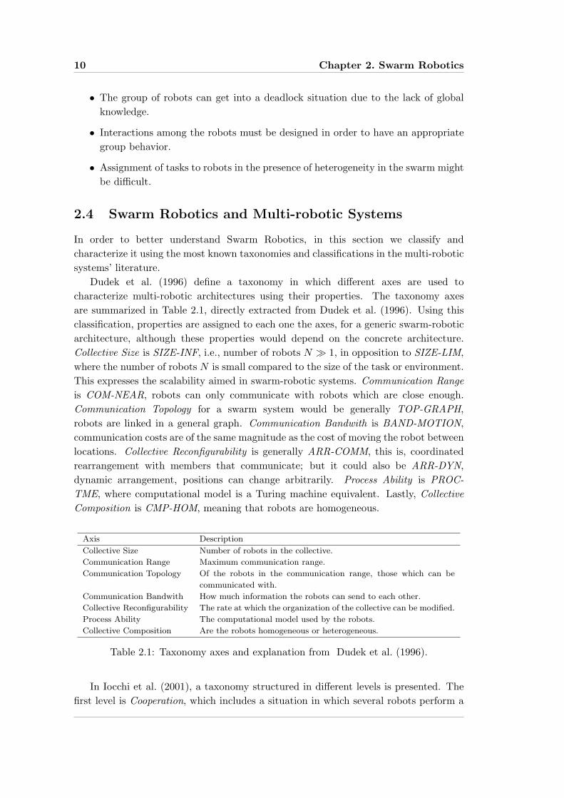
Dudek et al. (1996) define a taxonomy in which different axes are used tocharacterize multi-robotic architectures using their properties. The taxonomy axesare summarized in Table 2.1, directly extracted from Dudek et al. (1996). Using thisclassification, properties are assigned to each one the axes, for a generic swarm-roboticarchitecture, although these properties would depend on the concrete architecture.Collective Size is SIZE-INF, i.e., number of robots N À 1, in opposition to SIZE-LIM,where the number of robots N is small compared to the size of the task or environment.This expresses the scalability aimed in swarm-robotic systems. Communication Rangeis COM-NEAR, robots can only communicate with robots which are close enough.Communication Topology for a swarm system would be generally TOP-GRAPH,robots are linked in a general graph. Communication Bandwith is BAND-MOTION,communication costs are of the same magnitude as the cost of moving the robot betweenlocations. Collective Reconfigurability is generally ARR-COMM, this is, coordinatedrearrangement with members that communicate; but it could also be ARR-DYN,dynamic arrangement, positions can change arbitrarily. Process Ability is PROC-TME, where computational model is a Turing machine equivalent. Lastly, CollectiveComposition is CMP-HOM, meaning that robots are homogeneous.
Axis Description
Collective Size Number of robots in the collective.
Communication Range Maximum communication range.
Communication Topology Of the robots in the communication range, those which can be
communicated with.
Communication Bandwith How much information the robots can send to each other.
Collective Reconfigurability The rate at which the organization of the collective can be modified.
Process Ability The computational model used by the robots.
Collective Composition Are the robots homogeneous or heterogeneous.
Table 2.1: Taxonomy axes and explanation from Dudek et al. (1996).
In Iocchi et al. (2001), a taxonomy structured in different levels is presented. Thefirst level is Cooperation, which includes a situation in which several robots perform a

2.4. Swarm Robotics and Multi-robotic Systems 11
common task. Second level is Knowledge, which distinguishes whether robots know ofthe existence of other robots (Aware) or not (Unaware). Third level is Coordination,to differentiate the degree in which robots take into account the actions executedby other robots. According to the authors of the taxonomy this can be: StronglyCoordinated, Weakly Coordinated or Not Coordinated. The last level is Organization,which distinguishes between Centralized systems, where there exists a robot that isin charge of organizing other robots’ work, and Distributed systems, where robots areautonomous in their decisions, i.e., there are no leaders. According to this taxonomy,swarm-robotic systems are: Cooperative, Aware, Strongly Coordinated (they could alsobe Weakly Coordinated), and Distributed. A schematic of the taxonomy is shown inFigure 2.1, where for each level the corresponding type of system is marked in darkgrey for a swarm-robotic system.
Figure 2.1: Taxonomy from Iocchi et al. (2001). For each level the corresponding typeof system is marked in dark grey for a swarm-robotic system.
In Cao et al. (1997), a not so complete taxonomy is defined. It differentiatesamong centralized and decentralized architectures. Decentralized can be distributed,if all robots are equal with respect to control; or hierarchical if there exists a localcentralization. It also identifies between homogeneous and heterogeneous individuals.Using this taxonomy swarm systems are: decentralized, distributed, and homogeneous.It is not the intention of this chapter to survey the multi-robotic systems in general, butswarm-robotic systems. For a broader view of multi-robotic systems interesting surveyscan be found in: Martinoli (1999), Iocchi et al. (2001), Arai et al. (2002) and Parker(2008).
Anyway, it is worth to list here the advantages and drawbacks of multi-roboticsystems, since they can be extrapolated to swarm-robotic systems. We borrow herefrom Arkin (1998) a list of advantages and disadvantages of multi-robotic systemscompared to single-robot systems. Advantages of multi-robotic approaches are:
• Improved performance: when tasks can be decomposable, and a divide andconquer approach is appropriate. Using parallelism, groups can make tasks to be
12 Chapter 2. Swarm Robotics
done more efficiently.
• Task enablement: groups of robots can do certain tasks that are impossible for asingle robot.
• Distributed sensing: the range of sensing of a group of robots is wider than therange of a single robot.
• Distributed action: a group a robots can actuate in different places at the sametime.
• Fault tolerance: under certain conditions, the failure of a single robot within agroup does not imply that the given task can not be accomplished, thanks to theredundancy of the system.
Drawbacks are:
• Interference: robots in a group can interfere between them, due to collisionsocclusions, etc.
• Uncertainty concerning other robots’ intentions: coordination requires to knowwhat other robots are doing. If this is not clear robots can compete instead ofcooperate.
• Overall system cost: the fact of using more than one robot can make theeconomical cost bigger. This is ideally not the case of swarm-robotic systems,which intend to use many cheap and simple robots which total cost is under thecost of a more complex single robot carrying out the same task.
2.5 Experimental Platforms in Swarm Robotics
In this section, the different robotic platforms used in the most relevant swarm-roboticexperiments are described. In Section 2.5.1 different robots and their characteristicsare summarized, while the most used simulators are described in Section 2.5.2.
2.5.1 Robotic Platforms
Several robotic platforms used in swarm-robotic experiments in different laboratoriesare summarized in Table 2.2. These platforms are:
• Khepera robot (Mondada et al., 1999), for research and educational purposes,developed by Ecole Polytechnique Federale de Lausanne (EPFL, Switzerland),widely used in the past, nowadays has fallen in disuse;
• Khepera III robot1 (Pugh et al., 2009), designed by K-Team together with EPFL;
• e-puck robot2 (Mondada et al., 2009), designed at EPFL for educational purposes;1http://www.k-team.com2http://www.e-puck.org
2.5. Experimental Platforms in Swarm Robotics 13
• The miniature Alice robot (Caprari and Siegwart, 2005) also developed at EPFL;
• Jasmine robot3 (Kornienko et al., 2005), developed under the I-swarm project;
• I-Swarm robot4 (Valdastri et al., 2006), very small, also developed by the I-swarmproject;
• S-Bot5 (Mondada et al., 2005), very versatile, with many actuators, developed inthe Swarm-bots project;
• Kobot6 (Turgut et al., 2007), designed by Middle East Technical University(Turkey);
• SwarmBot7 (McLurkin, 2004), designed by i-Robot company for research.
In Table 2.2, the column Relative Positioning System indicates if the robots possessthe ability to determine the relative positions of their nearby robots. This sensor isquite useful and necessary in many swarm-robotic tasks. Some of them are based onthe emission of an infrared signal by a robot and the estimate of the distance by itsneighbors depending on the strength of the received signal (Pugh et al., 2009; Gutierrezet al., 2008). Others work by emitting an ultrasound pulse at the same time than aradio signal, and estimating the distance taking into account the time difference in thereception of both signals (Spears et al., 2007; Navarro-Serment et al., 1999). There arealso robots that use a camera to detect and estimate the position of nearby robots thatare equipped with markers (Nouyan et al., 2008; Parker et al., 2003; Das et al., 2002).
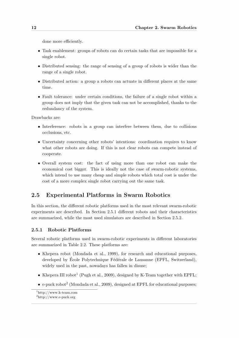
Pictures of of all the robots are shown in Figure 2.2. The Khepera III is the onlyrobot not shown; its description together with the corresponding figure are presentedin Appendix A.
2.5.2 Simulators
There exist many mobile robotic simulators available which can be used for multi-robotic experiments, and more concretely for swarm-robotic experiments. They differnot only in their technical aspects but also in the license and cost. We summarizethem, along with comments on their use on swarm-robotic applications in the followingparagraphs:
Player/Stage/Gazebo 8 (Gerkey et al., 2003) is an open source simulator withmulti-robotic capabilities and a wide set of available robots and sensors readyto use. The use for swarm-robotic experiments is analysed for 2D simulationsby Vaughan (2008), with very good results. Runtime scales approximately linearly
3http://www.swarmrobot.org4http://www.i-swarm.org5http://www.swarm-bots.org6http://www.kovan.ceng.metu.edu.tr7http://www.irobot.com8http://playerstage.sourceforge.net

14 Chapter 2. Swarm Robotics
Nam
eSize
(mm
)A
ctuato
rsC
om
putin
gSen
sors
Com
munica
tions
Rela
tive
Dev
elopm
ent
(dia
m.)
or
Capabilities
Positio
nin
g
(l.x
w.)
System
Khepera
55
Wheeled
Moto
rola
8IR
RS232
-R
esearch
(diff
erentia
ldriv
e)M
C68331
Wired
link
Com
mercia
l
Khepera
III120
Wheeled
PX
A-2
55
(400
MH
z)11
IRW
IFI
Expansio
nR
esearch
(diff
erentia
ldriv
e)Lin
ux
&dsP
ICs
5U
ltraSound
&B
lueto
oth
(IRbased
)C
om
mercia
l
e-p
uck
75
Wheeled
dsP
IC11
Infra
Red
(IR)
Blu
etooth
Expansio
nO
pen
Source
(diff
erentia
ldriv
e)C
onta
ctrin
g(IR
based
)C
om
mercia
l
Colo
rca
mera
Resea
rch&
Edu.
Alic
e20x20
Wheeled
Micro
chip
PIC
IRP
roxim
ity&
Lig
ht
Radio
-R
esearch
(diff
erentia
ldriv
e)Lin
ear
Cam
era(1
15
Kbit/
s)N
on
com
mercia
l
Jasm
ine
23X
23
Wheeled
2A
TM
ega
8IR
IRIn
tegra
tedO
pen
Source
(diff
erentia
ldriv
e)m
icroco
ntro
llers(IR
based
)R
esearch
I-Sw
arm
3x3
Micro
legged
aa
a-
Resea
rch
robot
Non
com
mercia
l
S-B
ot
120
Wheeled
XScla
e(4
00M
hz)
15
Prox
imity
WIF
IC
am
eraB
ased
Resea
rch
(diff
erentia
ldriv
e)Lin
ux
PIC
sO
mniC
am
eraN
on
com
mercia
l
2G
rippers
Micro
phone,
Tem
p.
Kobot
120
Wheeled
PX
A-2
55
(200M
Hz)
8IR
Zig
bee
Integ
rated
Resea
rch
(diff
erentia
ldriv
e)&
PIC
sC
olo
rC
am
era(IR
based
)N
on
com
mercia
l
Sw
arm
Bot
127x127
Wheeled
AR
M(4
0M
hz)
IR,Lig
ht
senso
rsIR
based
Integ
rated
Resea
rch
(diff
erentia
ldriv
e)&
FP
GA
200
kgate
Conta
ct,C
am
era(L
oca
l)(IR
based
)N
on
Com
mercia
l
Table
2.2:Sum
mary
ofthe
main
roboticplatform
sused
insw
armexperim
ents.aIn
form
atio
nnot
availa
ble.

2.5. Experimental Platforms in Swarm Robotics 15
(a) Kobot robot. (b) S-bot robot.
(c) SwarmBot robot. (d) E-puck robot. (e) Khepera robot.
(f) Jasmine robot. (g) Alice robot. (h) I-swarm robot.
Figure 2.2: Images of the main robotic platforms used in swarm experiments.
with population sizes up to at least 100,000 simple robots. It works on real timefor 1000 robots running a simple program. It is a good solution for swarm roboticexperiments.
Webots 9 (Michel, 2004) is a realistic, commercial mobile simulator that allows multi-robot simulation, with already built models of real robots. It is 3D, simulating
9http://www.cyberbotics.com
16 Chapter 2. Swarm Robotics
physics and collisions. It has been used in the experiments performed in thisThesis. According to our experience, its performance when working with morethan 100 robots decreases very fast, making the simulations with a large numberof robots difficult.
Microsoft Robotics Studio (Jackson, 2007) is a simulator developed by MicrosoftCorporation. It allows multi-robotic simulation. We do not know about theexistence of simulations with large amounts of robots. It requires a Windowsplatform to be run.
SwarmBot3D (Mondada et al., 2005) is a simulator for multi-robotics but designedspecifically for the S-Bot robot of the SwarmBot project.
2.6 Experimental Basic Behaviors and Tasks in Swarm
Robotics
A collection of the most representative experimental works in Swarm Robotics isdepicted in this section. Some of the works are also explained in Bayindir and Sahin(2007), which constitutes a good review on the field. Here, the different experimentalresults are organized in another way, grouping them depending on the tasks or behaviorscarried out by the swarms. Some of the behaviors, such as aggregation and collectivemovement, are quite basic and constitute a previous level for more complex tasks. Thedifferent behaviors and tasks are presented in increasing order of complexity.
2.6.1 Aggregation
In order to perform other tasks, such as collective movement, self-assembly and patternformation, or to exchange information, robots must initially gather. This aggregationproblem has been studied from a swarm-robotic approach by several researchers.
Trianni et al. (2003) perform experiments using an evolutionary algorithm onsimulated S-Bot robots. The sensory inputs are the proximity sensors and themicrophones. The actuators are the motors and the speakers. One of the evolvedsolutions is scalable. Bahgeci and Sahin (2005) also use evolutionary algorithms andsimulated S-bot robots, leading to scalable results, although their work is rather focusedon evolutionary algorithms than on aggregation.
Soysal and Sahin (2007) use an algorithm based on a probabilistic finite statemachine for aggregation. They develop a macroscopic model of it and compares itwith simulation results. Dimarogonas and Kyriakopoulos (2008) propose a distributedaggregation algorithm based on potential functions consisting on: a repulsive force forobstacle avoidance and a attractive force for aggregation. They analyse mathematicallyits convergence and carry out simulated experiments with nine robots. Lastly, Garnieret al. (2005) implement a biological model based on cockroach aggregation on Alicerobots.

2.6. Experimental Basic Behaviors and Tasks in Swarm Robotics 17
2.6.2 Dispersion
The aim of dispersion is to distribute the robots in space to cover it as much area aspossible, usually without losing the connectivity between them. The swarm can work,when dispersed, as a distributed sensor, but also as a means for exploration.
Dispersion has been studied by different researchers both using real robots and insimulation. Howard et al. (2002) present a potential field algorithm for the deploymentof robots, in which robots are repelled by obstacles and other robots. The approach isdistributed, and does not require centralized localization, leading to a scalable solution.The work is conducted only in simulation.
In Ugur et al. (2007), the authors propose and test in simulation a distributedalgorithm for dispersion based on the read wireless intensity signals and a potentialfield approach. According to them, and although robots do not have informationabout the bearing to neighboring robots, the algorithm successfully disperses the robots.Ludwig and Gini (2007) and Damer et al. (2006) also only use the wireless intensity fordispersion of a swarm of robots. They use a more elaborated algorithm that takes intoaccount a graph of the neighboring robots and the received signal intensities. Theyreach successful results in more complicated environments than the proposed in Uguret al. (2007). The fact that just wireless signal intensities are needed in these algorithmsmakes them quite attractive since they can be used with very simple robots not providedwith relative positioning systems.
McLurkin and Smith (2007) show the performance of a set of distributed algorithmsfor the dispersion of a large group of robots, where only inter-robot communicationsand sensing of other robots’ positions is used. The network connection of the swarm ismaintained, creating a route to the initial positions where chargers were placed. Thedispersion allows robots to explore large indoor environments. Experiments were runwith up to 108 real SwamBots, showing the algorithm’s scalability.
In Schwager et al. (2008) a distributed algorithm for dispersing a set of robots in theenvironment at the same time that robots aggregate in areas of interest, is presentedand tested. Experiments done with 16 real SwarmBot robots show the success of thealgorithm.
The coverage problem is related to dispersion. Robots need to disperse and detectthe borders of the environment. Correll et al. (2006) present a set of distributed andscalable algorithms for covering the boundaries of elements placed in a regular pattern.They show based on experimental results and using up to 30 Alice robots that coverageperformance is improved with increasing number of robots.
2.6.3 Pattern Formation
Pattern formation is the problem of creating a global shape by changing the positionsof the individual robots. Since we are here interested in a swarm-robotic approach, theexplained examples will have just local information.
In Fujibayashi et al. (2002), a swarm of particles form a lattice with both an internaland external defined shape. All the rules that make the particles/robots to aggregate in
18 Chapter 2. Swarm Robotics
the desired formation are local, but a global external shape emerges, without having anyglobal information. The algorithm uses virtual springs between neighboring particles,taking into account how many neighbors they have.
Martinson and Payton (2005) describe an algorithm that using a common referenceorientation for the robots and local control laws acting in orthogonal axes creates squarelattices.
Chaimowicz et al. (2005) show an algorithm for placing robots in different shapesand patterns defined by implicit functions. Robots use a distributed approach basedon local information to place themselves in the desired contour. Algorithms are testedboth in simulation and with real robots.
In Christensen et al. (2007, 2008), a framework to assemble a swarm of robots givena morphology is shown. Using the robots’ capability of attaching they demonstrate howS-bot robots self-assemble forming global morphologies. The algorithm is completelydistributed, and just local information is used.
2.6.4 Collective Movement
This is precisely the aim of study of this Thesis, namely the collective movement ofrobots from a swarm-robotic perspective, which focuses on the scalability in the numberof robots. It can also serve as a basic behavior for more complicate tasks. A review ofthis field is explained in more detail in Chapter 3.
2.6.5 Task Allocation
The problem of labor division is not a task as the previous one, but a problem that canarise in multi-robotic systems and particularly in Swarm Robotics.
Jones and Mataric (2003) present a distributed and scalable algorithm for labordivision in swarms of robots. Each robot maintains a history of the activities performedby other robots based on observation, and independently performs a division of laborusing this history. It then can modify its own behavior to accommodate to this division.
In Ducatelle et al. (2009), authors propose two different methods for task allocationin a robotic swarm. Tasks are previously announced by certain robots and a numberof them must attend to them simultaneously. The first algorithm is based on a gossipcommunication scheme, and it has better performance than the other, but due tolimited robustness to packet loss it might be less scalable. The second is simple andreactive, based on interaction through light signals.
McLurkin and Yamins (2005) describe four different algorithms for task allocationand test them using 25 SwarmBot real robots. The four of them result successful andscalable, although needing of different communication requirements.
In Groß et al. (2008), a group of robots must solve a complex foraging task thatis divided in a collection of sub-task. The authors propose and test with real robotsa distributed algorithm based on a state machine that solves the main problem byself-assigning each robot a desired task.
2.6. Experimental Basic Behaviors and Tasks in Swarm Robotics 19
2.6.6 Source Search
Swarm Robotics can be very useful in search tasks, especially those in which the spatialpattern of the source can be complex as in the case of sound or odor. The odorlocalization problem is studied in Hayes et al. (2003), where robots look for the odorsource using a distributed algorithm. They conducted experiments both in simulationand with real robots.
In Hurtado et al. (2004), authors describe and test a distributed algorithm forlocalizing stationary, time-invariant sources. They use feedback controls motivatedby function minimization theory. They explore two situations: one with globalcommunications, in which robots are able to find the global maximum source; anda second one restricted to local communication, where local maxima are found.Experiments are run in simulation.
2.6.7 Collective Transport of Objects
Swarm Robotics is very promising in solving the problem object transportation. Theuse of many robots can represent an advantage because of cooperation handling oneobject. In addition, the possible parallelism dealing with different objects by severalrobots at the same time might improve the performance.
Kube and Bonabeau (2000) take as inspiration the ant collective transport of preys,where individuals wait for other mates if the transported object is too heavy. In theirexperiments, performed with real robots, a group of 6 robots is able to collectively pushan object towards a destination, in a purely distributed way.
Groß and Dorigo (2009) solve the problem of transporting different objects by groupsof S-Bot robots that self assemble to cooperate. The algorithms were synthesisedusing an evolutionary algorithm. The experimental results in simulation show that thealgorithm scales with heavier objects by using larger groups of robots (up to 16). Butthe performance does not scale with the group size, since the mass transported perrobot decreases with the number of robots.
In Decugniere et al. (2008), authors discuss and propose the collective transportof objects by collecting them and storing them for later transport. The robots of theswarm would have two different tasks: collecting the objects and placing them in a cart;and collectively move the cart carrying objects. Authors suggest that the performanceis super linear with the number of robots.
2.6.8 Collective Mapping
The problem of collective mapping has not yet been widely studied by the swarm-robotic community. In Howard et al. (2004), a set of algorithms for the explorationand mapping of big indoor areas using large amounts of robots is described. In theirexperiments, they use up to 80 robots spread in a 600m2 area. Nevertheless, themapping is carried out by two groups of two robots that eventually exchange andmerge their maps, so it can not be considered swarm mapping.
20 Chapter 2. Swarm Robotics
Rothermich et al. (2005) propose and test (in simulation and with real robots) amethod for distributed mapping using a swarm of robots. Each robot can assumetwo roles: moving or landmark that are exchanged for the movement of the swarm.In addition, robots have a certain confidence in their localization estimated position.Using this information, localization estimates of other robots and sensor measurementsthey build a collective map.
2.7 Towards Real World Applications
In the first sections of this chapter many interesting and promising properties of SwarmRobotics have been enlightened. Nevertheless, currently there exist no real commercialapplications. The reasons for it are varied. Sahin and Winfield (2008) enumerate threeof them:
Algorithm Design. Swarm Robotics must design both the physical robots and thebehaviors of the individual robots, so the global collective behavior emerges fromtheir interactions. At the moment, no general method exists to go from theindividuals to the group behavior.
Implementation and Test. The use of many real robots needs of good laboratoryinfrastructure to be able to perform experiments.
Analysis and Modelling . Swarm-robotic systems are usually stochastic, non-linear,so building mathematical models for validation and optimization is hard. Thesemodels might be necessary for creating safety real world applications.
Winfield et al. (2005) discus the concept of swarm engineering, studying thedependability of swarm-robotic systems through a case of study. According to them,some of the future work needed from a dependability point of view is:
• Mathematical modelling of swarm-robotic systems.
• Work on safety analysis at robot and swarm level.
• Develop an approach to the design of emergence.
• Develop methodologies and practices for the testing of swarm systems.
Higgins et al. (2009) address the main security challenges that swarm-roboticsystems should face in a future. They state that due to the simplicity of swarm-roboticarchitectures they have to deal with the following problems:
• Physical capture of the robots;
• Identity and authentication, robot must know if it is interacting with a robotfrom its swarm or from an intruder robot;
• Communication attacks, communications can be intercepted or disturbed by anattacker.

2.8. Summary 21
The possible real applications of Swarm Robotics will take special importance whenrobots get to be mass produced and the costs of building swarms of robots decrease.This is the objective of I-swarm project (Seyfried et al., 2005) which aimed at buildinga swarm of micro robots. The development of technologies such as MEMS (Micro-Electro-Mechanical Systems) will allow to create small and cheap robots.
Swarm robots can perform tasks in which the main goal is to cover a wide region.The robots can disperse and perform monitoring tasks, for example in forests, lakes,etc. It can be really useful for detecting hazardous events, like a leakage of a chemicalsubstance. The main advantage over a sensor network is that the swarm can move andfocus on the problem and even act to prevent the consequences of that problem.
In this way swarms of robots can be really useful for dangerous tasks. For examplefor mining detection and cleaning. It can be more useful than a unique specializedrobot, mainly because of the robustness of the swarm: if one robot fails and the mineexplodes, the rest of the swarm continues working. In the case of a single robot this isnot possible.
The number of possible applications is really promising, but still the technologymust firstly be developed both in the algorithmic and modelling part, and also in theminiaturization technologies.
2.8 Summary
In this chapter, an overview of Swarm Robotics has been given, since it serves as a frameand inspiration for the collective movement algorithms developed in this Thesis. Thefirst sections have made an introduction to the topic, showing its main properties andcharacteristics and placing the field in relation to more general multi-robotic systems.The main tasks and experimental results in Swarm Robotics and the platforms usedhave been summarized. Lastly, the future promising applications together with theproblems to overcome in order to reach them have been explained.
22 Chapter 2. Swarm Robotics
Chapter 3
Collective Movement
This afternoon, on Cavenham Heath, a large band of rooks (severalhundreds) kept alternately hovering over, coming down amidst and flyingup from an expanse of withered bracken. They all rise instantaneouslyand simultaneously in a dense, black cloud, generally at fairly regularintervals of two or three minutes or so, but sometimes more quickly oralmost immediately on going down. I can see or hear nothing to suggest asignal given in any manner either by a leader or sentinels (nor are these tobe seen), and that the whole of them do not rise, each time, because a fewor some do, seems proved by the fact that such few or some are, betweenflight and flight, in a constant motion, rising, hovering and flying a littlefurther over the heads of the majority, amongst whom the re-alight and whoare not thereby affected. Moreover, as I say, the major risings are almostalways together.
Thought-Transference (or What?) in Birds (1931) - Edmund Selous
3.1 Introduction
In this chapter we intend to do a review on different types of collective movement,giving special attention to collective movement in mobile robots, since it is the the aimof the Thesis. Collective movement can be understood as the phenomenon seen whena set of individuals move together as a group in a cohesive way. It can be observed innature: in fish schools, flocks of birds, herds of wildebeests, etc. People, under certaincircumstances, also behave in similar manners, like in demonstrations, or crows walkingtowards mass gatherings like in concerts or sport events.
Collective movement in artificial systems has been designed for several purposes bydifferent communities. Video game and film industries simulate crowds of people andgroups of animals moving together in order to show realistic animations. Collectivemovement of mobile robots has been studied in the past two decades by many roboticsresearchers, adopting different approaches. This behavior can be considered a task initself in order to move a group of robots from one place to another, but also can be used
24 Chapter 3. Collective Movement
in more complicated and useful applications such as collective source search, collectivemapping, collective transportation.
The rest of the chapter is organized as follows. Section 3.2 performs a review ondifferent collective movement architectures, classifying and characterizing them. It alsodescribes the different basic functions that a group of mobile robots moving togethermight perform. In addition potential applications of collective movement of mobilerobots are described. Some examples of collective movement in nature are explained inSection 3.3, while another example of collective movement where cyclists ride togetheris described in Section 3.4. Lastly, a summary of the chapter is given in Section 3.5.
3.2 Collective Movement in Robotics
Collective movement of mobile robots is the problem of how to control a group ofrobots making them move as a group, in a cohesive way and towards a commondirection. Historically collective movement of robots has been classified into two types:formations and flocking. In the former, robots must maintain pre-determined positionsand orientations among them. On the other hand, in flocking, robots’ relative positionsare not strictly enforced. The differences and characteristics of both types are betterexplained in Section 3.2.1.
The first work in artificial flocking was a computer graphic animation of a group ofbirds by Reynolds (1987). With just three simple local rules, the artificial birds wereable to move as a cohesive group:
1. Collision Avoidance, avoiding collisions with other flock-mates;
2. Velocity Matching, matching velocity with nearby flock-mates;
3. Flock Centering, trying to stay close to neighboring flock-mates.
Collective movement architectures of mobile robots should ideally possess thefollowing desirable characteristics:
• Scalability with an increasing number of robots;
• Robustness to changes in the size of the group and single robot failures;
• Ability to create different external shapes and modify them dynamically;
• Obstacle avoidance at group level;
• Ability to split in smaller groups, and rejoin small group to form larger ones.
• Use local rules based on local information and communication, in order tofacilitate scalability.
• In the case of formations, robots should not need any predefined positions.

3.2. Collective Movement in Robotics 25
3.2.1 Classifications
As has been said in the previous section, collective movement problems are classifiedinto two categories: formation control and flocking. The formation control or robotformations problem consists in how to coordinate a group of robots making themmaintain a determined position while moving in the environment. Sometimes justthe relative positions between robots are determined, in other occasions also a desiredoutline must be fulfilled.
Flocking is the problem of creating and moving a group of robots when the shapeand relative positions between the robots are not important. In a flocking problem theexternal shape could also be controlled but it is not often done.
Flocking of robots is interesting because it allows big groups of robots to move usingdecentralized control and local sensing. But, in some applications, formations can be anadvantage compared to flocking, when fixed positions are necessary. Robots might havedifferent roles depending on their positions in the formation, e.g., those in the boundaryarea of the formation may be in charge of mapping and deciding the movement directionwhile the rest could be in charge of sensing other environment variables such as sound,temperature or odor. Since robots may have different capabilities, they should remainat different positions within the formation. In addition, keeping fixed positions makesit easier to maintain a map of the positions of the robots relative to themselves, and touse this structure for cooperative sensing.
Some formation architectures or algorithms create lattices given by the positions oftheir robots. The robots form a regular pattern made of squares, rectangles or triangles.Lattices formed by triangles are also called hexagonal, because six triangles form anhexagon. Usually these formations are created using potential fields between nearbyrobots. Some lattice algorithms are not so strict with the positions of the robots, andjust try to maintain a desired inter-robot distance which forms a triangular lattice, butgive a priority to the movement. The group moves while trying to maintain an inter-robot distance, so they can be considered as flocking and not strictly as a formation.For instance, in the case of the architecture proposed in this Thesis and described inChapter 6, robots start moving as a group even if the positions of the robots are notsatisfactory. During the initial moments of this movement robots reallocate to thedesired positions, so it can be considered a kind of lattice-flocking, even if most ofthe time the desired positions are respected. On the other hand, in lattice formationsas in the case described in Navarro et al. (2009), robots first place in the appropriatepositions and then start moving. The disadvantage is that the movement is not smoothsince from time to time some robots stop their movement to place themselves in theright positions.
In Figure 3.1, a schematic of each of the three types of collective movement types,flocking, formations and lattices (formation or flocking), are depicted.
Robot formations are classified by Balch and Arkin (1998) into the following threegroups, which we comment and analyze here:
• Unit-center-referenced. A center is computed independently by each robot by

26 Chapter 3. Collective Movement
(a) Formation. (b) Triangular
lattice.
(c) Flock.
Figure 3.1: Schematics showing different types of collective movements: (a) wingformation, (b) lattice (flocking or formation) and (c) flocking.
averaging the positions of all robots, and then each robot determines its ownposition relative to this center. This kind of formation is not scalable sinceit implies that each robot must know the position of every other robot in theformation, which it is not practical at all.
• Leader-referenced. Each robot maintains a position with respect to a leader robot.The leader does not follow any robot, and is in charge of path planning. As theprevious case, scalability is a problem since all the robots must know the positionof the leader.
• Neighbor-referenced. Each robot maintains a position referred to other robot. Inthis way, chains or tree structures are formed where one robot follows anotherone. Depending on the distance and angles to neighbors different structuresarise: diamond, wedge, column, etc. If one robot is followed by more thanone robot, branches can be created and more complex structures arise. Theinternal structure and the external shape cannot be differentiated in these cases.Scalability in this case might be also difficult, since the position error canpropagate cumulatively from one robot to others.
According to Balch and Arkin (1998) in the Neighbor-referenced model each robotdetermines its position referred to other robot, but there are many architectures andalgorithms in which robots calculate their positions depending on the positions ofseveral neighbors. We can include these algorithms also in the Neighbor-referencedtype. This algorithms create formations of lattice type like the ones explained before,but also could create more complex structures. Different architectures differ on theattracting functions and the way to chose neighbors. If these algorithms are basedon local control and sensing they can scale with increasing number of robots, sincerobots determine their positions based on more than one robot so the error does notpropagate so fast. In principle the global shape of the formation is not pre-specifiedand is determined solely by local interactions, unless another controller is introducedto modify it.
According to the type of controllers to allow collective movement they can bedistributed or centralized. Centralized controllers do not ensure scalability. The samecan be said about communications and sensing.

3.2. Collective Movement in Robotics 27
Most of the examples in the literature imply movement in two dimensions, but thereare also algorithms and frameworks for three dimensional collective movement, whichallow the control of unmanned aerial vehicles or autonomous underwater vehicles.
Formations explained and described in this chapter are not related to the formationproblems where the group of robots remains static, which are more closely related topattern formation, explained in Section 2.6.3.
3.2.2 Functions of a Group of Robots Moving Collectively
In order to better understand the potential possibilities of collective movement of mobilerobots, and to be able to compare and understand the different architectures reviewedin Section 3.2.3, some basic functions, which can be performed by a group of robotsmoving together, are explained in the next sections helped by the use of sketches thatshow the positions of robots with time.
3.2.2.1 Aggregation
Aggregation is the process in which robots spread in the environment group together.It is not a function of collective movement, but a previous step necessary for collectivemovement. In Figure 3.2, an aggregation process over time is depicted. The last steprepresents alignment of the robots for later movement.
Figure 3.2: Schematic showing the aggregation mechanism of a group of robot and alater alignment of the individuals.
3.2.2.2 Moving to a Desired Place
Moving from one place to another is a basic function that a group of robots mightperform, the path followed can be decided or planned by the group of robots or byone of them, or can be previously provided by a user. In Figure 3.3, the collectivemovement from one point to another following a pre-defined path is shown.
3.2.2.3 Obstacle Avoidance
Robots must avoid collisions individually for safety reasons, but it is also convenientfor a group of robots to be able to avoid obstacles at group level. This allows them

28 Chapter 3. Collective Movement
to maintain the group cohesive, avoiding undesired splits. In Figure 3.4, the obstacleavoidance at group level function is depicted in different time steps.
Figure 3.3: Schematic of a group of robots following a path together.
Figure 3.4: Schematic showing how a group of robots performs the obstacle avoidancefunction.
3.2.2.4 Splitting in Smaller Groups
For a group of robots moving together it can be useful or necessary to divide or splitinto two or more groups. This can allow them to overpass a large obstacle so that onegroup leaves the obstacle on its left and the other group leaves it on its right, as isshown in the schematic presented in Figure 3.5. The decision on when and how to splitmight depend on the number of robots, the desired task that the group must performor on the environment. For instance,a group of robots can split in subgroups for a moreefficient performance in searching tasks.
3.2.2.5 Rejoining Groups
Two or more groups of robots moving separately can rejoin eventually and becomea larger group that can behave as a single one. This can be useful if the task that
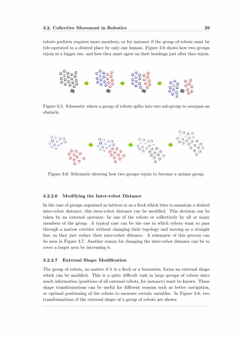
3.2. Collective Movement in Robotics 29
robots perform requires more members, or for instance if the group of robots must betele-operated to a desired place by only one human. Figure 3.6 shows how two groupsrejoin in a bigger one, and how they must agree on their headings just after they rejoin.
Figure 3.5: Schematic where a group of robots splits into two sub-group to overpass anobstacle.
Figure 3.6: Schematic showing how two groups rejoin to become a unique group.
3.2.2.6 Modifying the Inter-robot Distance
In the case of groups organized as lattices or as a flock which tries to maintain a desiredinter-robot distance, this inter-robot distance can be modified. This decision can betaken by an external operator, by one of the robots or collectively by all or manymembers of the group. A typical case can be the one in which robots want to passthrough a narrow corridor without changing their topology and moving as a straightline, so they just reduce their inter-robot distance. A schematic of this process canbe seen in Figure 3.7. Another reason for changing the inter-robot distance can be tocover a larger area by increasing it.
3.2.2.7 External Shape Modification
The group of robots, no matter if it is a flock or a formation, forms an external shapewhich can be modified. This is a quite difficult task in large groups of robots sincemuch information (positions of all external robots, for instance) must be known. Theseshape transformations can be useful for different reasons such as better navigation,or optimal positioning of the robots to measure certain variables. In Figure 3.8, twotransformations of the external shape of a group of robots are shown.
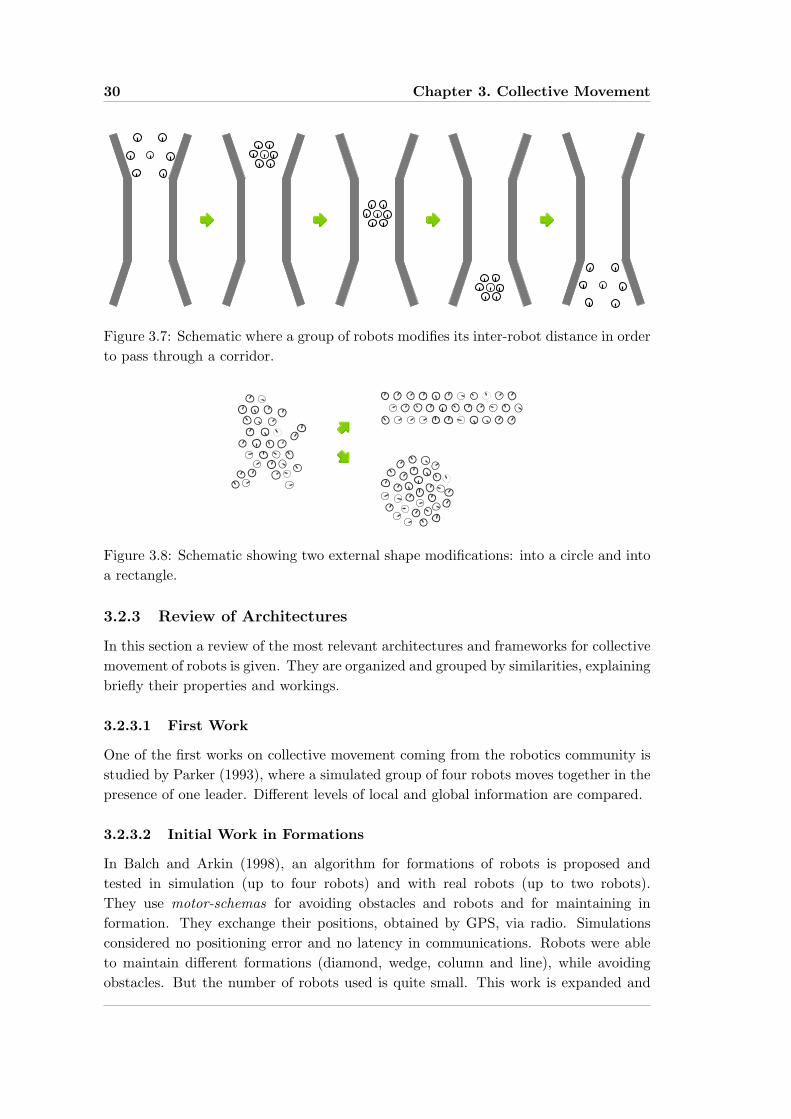
30 Chapter 3. Collective Movement
Figure 3.7: Schematic where a group of robots modifies its inter-robot distance in orderto pass through a corridor.
Figure 3.8: Schematic showing two external shape modifications: into a circle and intoa rectangle.
3.2.3 Review of Architectures
In this section a review of the most relevant architectures and frameworks for collectivemovement of robots is given. They are organized and grouped by similarities, explainingbriefly their properties and workings.
3.2.3.1 First Work
One of the first works on collective movement coming from the robotics community isstudied by Parker (1993), where a simulated group of four robots moves together in thepresence of one leader. Different levels of local and global information are compared.
3.2.3.2 Initial Work in Formations
In Balch and Arkin (1998), an algorithm for formations of robots is proposed andtested in simulation (up to four robots) and with real robots (up to two robots).They use motor-schemas for avoiding obstacles and robots and for maintaining information. They exchange their positions, obtained by GPS, via radio. Simulationsconsidered no positioning error and no latency in communications. Robots were ableto maintain different formations (diamond, wedge, column and line), while avoidingobstacles. But the number of robots used is quite small. This work is expanded and

3.2. Collective Movement in Robotics 31
improved in Balch and Hybinette (2000), where also motor schemas are used (herenamed social potentials), positioning robots with respect to more than one neighboringrobot through artificial attachment points. This allows them to create also latticeformations. Results are obtained only with simulation, with up to 32 robots. Not a lotof details are given in the results.
Fredslund and Mataric (2001) and Fredslund and Mataric (2002) propose and testan algorithm similar to the work of Balch and Arkin (1998) but making it scalable sincerobots just need to know the relative position of one nearby robot and communicatewith it. Also diamond, wedge, column and line formations are created. Identificationnumbers are used, but robots are not enforced to occupy fixed positions (Fredslund andMataric, 2002).
3.2.3.3 More Advanced Formations
In Kostelnik et al. (2002), a similar algorithm also using local rules, this time basedon a layered architecture, is proposed and tested in simulation. The formation has thecapability of creating the previous explained formations. Experiments are performedin simulation with up to seven robots. Naffin and Sukhatme (2004) present also aleader-follower approach for creating formations (diamond, wedge, column and line).The novelty is that robots are able to optimize the formation by changing their roles. Inaddition, experiments are carried out also with four real robots. In Naffin and Sukhatme(2004), the stability of a simplified and modified similar controller is analyzed. Hsuand Liu (2005) propose a similar leader-follower architecture and analyze its resultsperformance and capabilities in more detail. Experiments are performed only insimulation.
3.2.3.4 Formations Based on Path Planning
Barfoot et al. (2002) propose and test a formation controller for collective movementbased on path planning of the trajectories of the individuals. Paths are calculatedoff-board and control signals are sent directly to the robots. Thus, the controlleris centralized knowing at every moment the position of every robot. Experiments areperformed using six real robots. Bhatt et al. (2004) also present a method for formationcontrol based on path planning. They take explicitly into account the nonholonomicconstraints of the differentially-driven robots used. Only simple case studies are tested.
3.2.3.5 Other Formation Algorithms
Chang and Fu (2008) present a control framework for collective movement in formationbased on a Lyapunov approach. The framework is tested in simulation using only threerobots. In Lawton et al. (2003), three different control strategies for the movementin formation of a set of robots are presented and tested. They also use a Lyapunovapproach. Experiments are carried out using three real robots.
In Pereira and Hsu (2008), a controller for the formation of robots modeled asEuler-Lagrange systems is presented and tested only in simulation. They use binary

32 Chapter 3. Collective Movement
adaptive control and artificial potential functions. Robots need to know the velocitiesof nearby robots, which makes the controller difficult to implement on real robots.
3.2.3.6 Reconfigurable Formations
Desai et al. (2001) propose and test a formation control strategy which allows changesin the shape of the formation. There is a leader robot and the control of the rest ofthe robots is based on a leader follower approach, where the leader is followed by oneor more robots, and these robots are followed by others. Depending on the leader-follower graph used different shapes arise. Changes of shape are performed by addingand deleting edges of the graph. The algorithm is tested in simulation using up to sixrobots. In Das et al. (2002), the change in the shape of the formation is performedby changing the control graph. The controller is distributed among the robots andaccording to the authors it is scalable with the number of robots. Tests are performedusing three real robots provided by omnidirectional cameras as sensors, but helped byoff-board computation on an external computer.
3.2.3.7 Initialising Formations
Lemay et al. (2004) propose a method to determine in a distributed manner the optimalpositions that robots must occupy in a formation depending on their initial positions.The method is tested in simulation and with real robots.
3.2.3.8 Formations Based on Common Coordinate System
Lee and Chong (2009) describe and test a new decentralized formation algorithm basedon a common coordinate system given by the position of a leader robot. It allows tocreate a wide variety of formations: circles, lattices, wings, columns, regular polygons,diamonds. The algorithm is tested both in simulation (12 robots) and in reality (fourrobots).
3.2.3.9 Scalable Lattice Formations
In Spears et al. (2004b,a, 2005), the Physicomimetics Framework (PF), which allows tocreate a self-organized formation by using control laws inspired by physics, is presentedand analyzed. The controller is fully decentralized; each robot perceives the relativepositions of its neighbors and reacts to attractive or repulsive forces, forming triangularlattices. The algorithm is scalable, working for dozens of robots. The bulk of the work inPF has been done in simulation, and robots are considered to be holonomic. In Spearset al. (2005), it is explained that PF is used with nonholonomic robots, but moving bymaking a rotational movement followed by a translation within a large time window.Such an approach would not be practical for most real-world formations, where thereaction time is a critical system attribute.
Lee and Chong (2008a) propose a distributed algorithm for collective movementbased on lattices. Its convergence is proved using Lyapunov’s theorem. It is tested in

3.2. Collective Movement in Robotics 33
simulations with up to 100 robots. In Lee and Chong (2008b), a similar algorithm isproposed allowing the split of groups to overpass obstacles. Its performance is testedonly in simulation.
In Lindhe and Johansson (2005) and Lindhe and Ogren (2005) a decentralizedalgorithm for the collective movement based on lattice formations is proposed. Thestability of the algorithm in a particular case of study is proven. Obstacle avoidance isimplemented by partitioning the plane into Voronoi regions. Tests are carried out onlyin simulation with up to 29 robots.
In Antonelli et al. (2010), a new approach for the coordination of multiplerobots, named Null-Space-based Behavioral control, is described. This description isaccompanied with two examples of collective movement: formation control (Antonelliet al., 2007) and flocking in lattices (Antonelli et al., 2008).
3.2.3.10 Graph Formalization of Formations
In Olfati-Saber and Murray (2002b), a graph based theoretical framework that formallydefines the formations of robots is presented. It allows to formulate stability problemsof formations, and to represent formally the split and rejoin functions of a group ofrobots. Part of this graph formalization is used in Olfati-Saber and Murray (2002a)in order to control a formation of robots using a distributed approach and potentialfunctions. Results are presented from only two simulated examples.
3.2.3.11 Collective Movement Based on Consensus
Consensus problems are those in which a set of inter-communicated agents must agreeon the value of a variable. This kind of problems are explained in more detail inSection 5.2. Several collective movement algorithms make use of consensus on thevelocities or headings of the robots in order to create the cohesive movement of thegroup.
In Tanner et al. (2003a), a flocking movement of a group of robots is created byusing a distributed controller based on attractive-repulsive forces and agreement onthe velocities among nearby robots. Consensus is obtained using an average function.The stability of the controllers under a fixed topology, i.e. neighboring robots do notchange, is proven and also qualitative results from a single simulation are presented.In Tanner et al. (2003b) the stability analysis is generalized to dynamic topologywhere connectivity among robots changes with time. More qualitative and quantitativeresults for experiments in simulation using similar controllers are shown in Tanner et al.(2003c).
Jadbabaie et al. (2003) study the collective movement of a group of robots whena consensus protocol is applied only to the headings. Different variations are studiedincluding one where one of the robots does not change its heading an tries to impose itto the rest of the group. All the analysis is performed theoretically and no simulationsor any type of experiments are carried out.
Olfati-Saber (2006) presents a set of distributed control algorithms for the collective
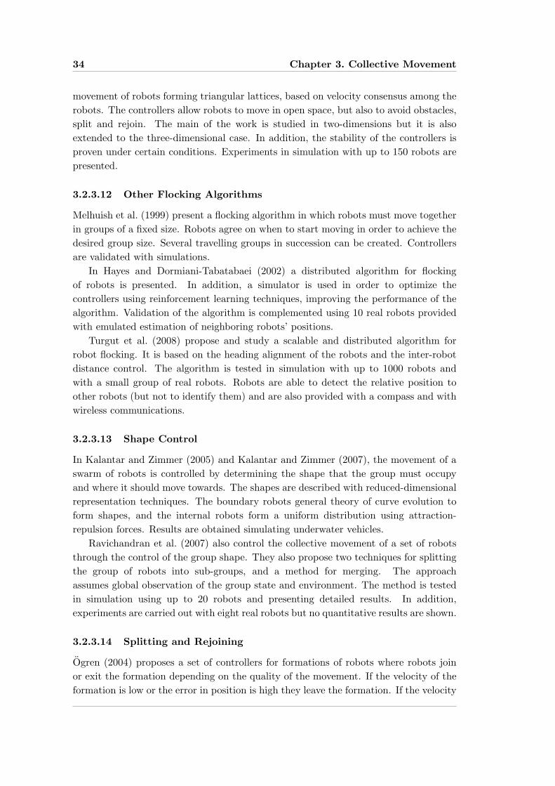
34 Chapter 3. Collective Movement
movement of robots forming triangular lattices, based on velocity consensus among therobots. The controllers allow robots to move in open space, but also to avoid obstacles,split and rejoin. The main of the work is studied in two-dimensions but it is alsoextended to the three-dimensional case. In addition, the stability of the controllers isproven under certain conditions. Experiments in simulation with up to 150 robots arepresented.
3.2.3.12 Other Flocking Algorithms
Melhuish et al. (1999) present a flocking algorithm in which robots must move togetherin groups of a fixed size. Robots agree on when to start moving in order to achieve thedesired group size. Several travelling groups in succession can be created. Controllersare validated with simulations.
In Hayes and Dormiani-Tabatabaei (2002) a distributed algorithm for flockingof robots is presented. In addition, a simulator is used in order to optimize thecontrollers using reinforcement learning techniques, improving the performance of thealgorithm. Validation of the algorithm is complemented using 10 real robots providedwith emulated estimation of neighboring robots’ positions.
Turgut et al. (2008) propose and study a scalable and distributed algorithm forrobot flocking. It is based on the heading alignment of the robots and the inter-robotdistance control. The algorithm is tested in simulation with up to 1000 robots andwith a small group of real robots. Robots are able to detect the relative position toother robots (but not to identify them) and are also provided with a compass and withwireless communications.
3.2.3.13 Shape Control
In Kalantar and Zimmer (2005) and Kalantar and Zimmer (2007), the movement of aswarm of robots is controlled by determining the shape that the group must occupyand where it should move towards. The shapes are described with reduced-dimensionalrepresentation techniques. The boundary robots general theory of curve evolution toform shapes, and the internal robots form a uniform distribution using attraction-repulsion forces. Results are obtained simulating underwater vehicles.
Ravichandran et al. (2007) also control the collective movement of a set of robotsthrough the control of the group shape. They also propose two techniques for splittingthe group of robots into sub-groups, and a method for merging. The approachassumes global observation of the group state and environment. The method is testedin simulation using up to 20 robots and presenting detailed results. In addition,experiments are carried out with eight real robots but no quantitative results are shown.
3.2.3.14 Splitting and Rejoining
Ogren (2004) proposes a set of controllers for formations of robots where robots joinor exit the formation depending on the quality of the movement. If the velocity of theformation is low or the error in position is high they leave the formation. If the velocity
3.2. Collective Movement in Robotics 35
is high and robots are in a good position in the formation they join it. The method istested only in simulation, with only one example.
In Chaimowicz and Kumar (2004), a method for splitting a group of robots andrejoining two groups of robots is explained. Each group of robots is leaded by an aerialblimp that tracks the robots. If two groups of robots have the same destination andone of the blimps is able to track both groups it will get in charge of both and rejointhe groups. If one group has to split into two sub-groups, the aerial blimp will leadone of them and ask a second blimp to track the other sub-group. As can be seen thehigh-level coordination is centralized in the aerial blimp and not distributed among therobots.
3.2.3.15 Collective Movement Using Intelligent Control
Pinciroli et al. (2008) present another distributed control algorithm for the formationof lattices. A genetic algorithm is used in order to optimize the parameters of thecontrollers.
Some researchers use fuzzy controllers for solving the collective movement problem,adopting different solutions. In Sisto and Gu (2006) and Bazoula et al. (2008), twodifferent fuzzy controllers for a leader-follower algorithm are presented. Bajec et al.(2005) present a fuzzy controller for flocking. All of them are only tested in simulation.
In Kwok et al. (2007), particle swarm optimization is used to optimize a formationcontrol algorithm. Experiments are tested only in simulation with few robots.
3.2.3.16 Collective Movement in 3 Dimensions
Moshtagh et al. (2006) study the flocking of a group of agents based on the observationof neighboring robots in the absence of communications, allowing planar and three-dimensional movement. Controllers are tested in simulation with up to four robots inthe three-dimensional case.
3.2.4 Applications
Most of the multi-robot applications can improve their performance by making use ofcollective movement. Some of this applications are enumerated here:
• Search and rescue operations, whose performance can be improved if robotsorganize in formations;
• Search of odor Hayes et al. (2002) or sound Pugh and Martinoli (2007).
• Control of arrays of satellites and unmanned aerial vehicles;
• Distributed sensor arrays, in which it is very important to set the appropriatedistances among them in order to have a better received signal;
• Future applications of autonomous highway vehicles, allowing cars to move in acoordinated way;

36 Chapter 3. Collective Movement
• Collective movement of objects;
• Environmental monitoring;
• Collective mapping Howard (2004).
3.3 Collective Movement in Animals
Collective movement can be observed in numerous species of animals. Certain interestcan be put into schools of fishes and flocks of birds since they have initially inspiredartificial collective movement and because some of the models used by the researchersstudying them are similar to the controllers used in robotics (Inada, 2001; Couzinet al., 2002; Viscido et al., 2005; Ballerini et al., 2008). Most of the proposed modelsare distributed, based only on neighboring information and leaderless. Not only fishesand birds move in groups but also herds of mammals (Gueron et al., 1996).
Heppner (1997) describes the collective movement of some type of birds, analysingits structure and dynamics. Geese usually fly in wedge formation, in a very perfectmanner. There are different theories for explaining this phenomenon, one of them isthe energy saving thanks to better aerodynamic properties.
According to Heppner (1997) researchers have different theories and models for theworkings of large flocks of starlings. Some researchers think that there are leaders in theflock, while other thinks that there are not. Some think that birds turn in synchronicitywhile other believe that these turns are produced in a wave manner that propagatesfrom some parts of the flock to others. A photograph of a large flock of this type isshown in Figure 3.9.
Figure 3.9: Flock of birds.
Fish schools can have different shapes and sizes, and have different functions likeavoiding predators or creating parabolic formations (in tuna schools) for cooperative

3.4. Other Collective Movements: Bicycle Critical Mass 37
hunting (Parrish et al., 2002; Sumpter, 2006). Partridge (1982) describes some of theevasive techniques fish schools exhibit when escaping from a predator, like the flashexpansion and the fountain effect. In Figure 3.10 a school of fishes is shown.
Figure 3.10: School of fishes.
3.4 Other Collective Movements: Bicycle Critical Mass
Critical Mass is a bicycling event in which cyclists gather to ride the streets of their cityin the absence of any leaders, and following a route that is generally not pre-specifiedbut chosen by those riders in the front part of the bunch. It took place for the first timein 1992 in San Francisco and it is currently celebrated as a monthly event in more than300 cities around the world (Madden, 2003; Mapes, 2009). The leaderless structure ofCritical Mass makes it difficult to assign it a goal, but one of the aims of these ridesis to promote the use of bicycles and to show that cycling is a valid transportationmethod in cities. The number of riders varies from dozens up to few thousands ofthem, depending on the city. In Figure 3.11 a picture of a Critical Mass event is shown.
Bicycles in the Critical Mass move following the traffic rules but acting as a group.This is different than normal traffic where cars (or bicycles) follow the traffic rules butthey move to different places, not acting as a group. Traffic rules in Spain considerthat a group of bicycles must follow traffic rules as if it is a unique vehicle.
In the Critical Mass events celebrated in Madrid in 2009, the group of bicycles oftensplit unintentionally into two or more sub-groups. The later rejoin into a single groupdid not always occur since cyclers in the front part of the group did not realize the splitand did not stop to wait for the groups in the back. On the other hand, some cyclers inthe Critical Mass events celebrated in Rome are equipped with handheld transceivers,allowing to communicate information between distant cyclers. If the group splits intotwo groups those cyclers in the back part of the second one can communicate the

38 Chapter 3. Collective Movement
Figure 3.11: Critical Mass event.
problem to those in the front part of the first group and make it stop to wait forthem. This need of communication in large groups might be taken into account whendesigning controllers for collective movement of robotic swarms.
3.5 Summary
In this chapter, a study of collective movement in robotic systems has been done. First,an introduction to the problem has been explained, followed by a set of classificationsof the different types of movements. The basic functions that a group of mobile robotsmoving together might perform is also given, followed by a review of the most relevantarchitectures. In addition, potential applications of collective movement of mobilerobots are described. The chapter ends with a brief description of collective movementfound in other areas out of the robotics research such as the one performed by animalgroups and groups of cyclists.

Part II
Main

Chapter 4
Metrics for Collective Movement
of Robots
I often say that when you can measure what you are speaking about, andexpress it in numbers, you know something about it; but when you cannotexpress it in numbers, your knowledge is of a meagre and unsatisfactorykind; it may be the beginning of knowledge, but you have scarcely, in yourthoughts, advanced to the stage of science, whatever the matter may be.
Electrical Units of Measurement - William Thomson, 1st Baron Kelvin
4.1 Introduction
In this chapter we intend to define and discuss a set of metrics to evaluate theperformance of collective movement of mobile robots. As stated in Bonsignorio et al.,the set of measurements used in robotic experiments to define its performance must beidentified and clearly motivated when reporting results. In order to compare differentalgorithms, it is necessary to use common metrics for the different algorithms. Thisset of metrics should go with a set of scenarios and tests, similar to those describedin Marjovi and Marques (2008), where the experiments should be carried out, in orderto have a benchmark.
The multi-robot research community working on formations and flocking of robotsdo not share a common set of metrics, and usually similar but not comparablemetrics are used. There are few works on defining metrics for collective movement,like Schneider et al. (2005) and Viscido et al. (2005), but the first does not cover someof the metrics that can measure collective movement, while the second is focused oncollective movement of fish schools. This is a reason to propose a more complete setof metrics oriented to analyse and discuss experiments on formations and flocking ofrobots. In principle the metrics are focused on 2 dimensions, but could be extrapolatedto 3-dimensional problems with formations of aquatic robots or autonomous flyingvehicles.
The basic mathematical notation used in this chapter and following chapters of the
42 Chapter 4. Metrics for Collective Movement of Robots
Thesis is defined in Section 4.2. The set of proposed metrics is defined and discussedin Section 4.3. Finally an overview of the chapter and conclusions can be found inSection 4.4.
4.2 Basic Definitions
We can define the complete group of robots under study as R = {..., ri, ...}, 1 ≤ i ≤ N ,where N is the number of robots. The position at time t of a single robot ri canbe defined with respect to an arbitrary reference frame by the pose vector ~ξi(t) =(xi(t), yi(t), θi(t))T , where xi(t) and yi(t) are the coordinates of a reference point ~pi ofthe robot ri, and θi describes the orientation of a frame attached to the robot withrespect to the reference frame, this is, its heading. The positions and heading of thegroup of robots R is then given by ~ξ(t) = (..., ~ξT
i (t), ...)T , 1 ≤ i ≤ N .The δ-neighborhood of a robot is defined as a set of robots that fulfill certain
conditions based on inter-robot distance, that depends on the parameter δ. The δ-neighborhood Ni,δ(t) of a robot ri is Ni,δ(t) = {rj |j 6= i, ‖~pi(t) − ~pj(t)‖ ≤ δ}, whereδ > 0 and it is set arbitrarily depending on the experiment under analysis.
The robots moving in formation or flocking communicate and detect the relativepositions of their neighbors under a certain range, building a graph that determines theconnectivity of the group. In Michael et al. (2008) the notion of dynamic undirectedgraph is described and some of its properties are explained, which will be heresummarized. A dynamic graph is defined as G(t) = (R, E(t)) where R = {..., ri, ...}, 1 ≤i ≤ N is the set of vertices or robots and E(t) = {(ri, rj)|ri, rj ∈ R} denotes the timevarying set of links such that: (ri, rj) ∈ E(t) if ‖~pi(t)−~pj(t)‖ ≤ range and (ri, rj) /∈ E(t)if ‖~pi(t) − ~pj(t)‖ > range, where range is the range of the communication andneighboring detection system. Since the communication is assumed to be bidirectionaland ‖~pi(t)− ~pj(t)‖ = ‖~pj(t)− ~pi(t)‖, then (ri, rj) ∈ E(t) if and only if (rj , ri) ∈ E(t), sothe graphs under study are undirected. According to the previous definition of Ni,δ itcan be pointed out that (ri, rj) ∈ E(t) if and only if j ∈ Ni,δ for a δ = range. If in G(t)there is a path (i.e., a sequence of distinct vertices such that consecutive vertices areadjacent) between any two of its vertices, then it can be said that G(t) is connected.
In order to compute the different proposed metrics, a sampled version of the vectorsand equations will be used, since both data acquisition and computation are discrete.The sample period used is T , while n indicates the sample number that correspondsto t = nT and M is the number of samples of a complete experiment. For instancethe pose vector ~ξi(t) of robot ri is expressed in its sampled form as: ~ξi[n] = ~ξi(nT ) =(xi(nT ), yi(nT ), θi(nT ))T = (xi[n], yi[n], θi[n])T .
4.3 Metrics
The proposed set of metrics seeks to be as complete as possible but also useful todetermine the performance of the different algorithms for the coordination of collectivemovement. Some of the metrics can be applied only to formations of robots or to

4.3. Metrics 43
flocking of robots, but not to both problems due to the different nature of them. Notall the metrics proposed have the objective of being used as a benchmark. There aresome that are useful to characterize the type of flock, but that can not be used to createa ranking.
The set of metrics has been divided in different subsets, grouping them accordingto their resemblances. They are defined and discussed in the following subsections.
4.3.1 Shape
In order to compute the metrics related to the shape of the group, the robots thatbelong to the boundary of the flock or formation must be identified. This can be doneusing convex hull (Graham, 1972) or α-shape (Edelsbrunner et al., 1983) algorithms,leading to different results in the metrics.
The convex hull of a set of points S, is the smallest convex polygon containing allthe points in S, and it is defined by the sub-set of points in S that are vertices of theconvex polygon. The algorithm described in Graham (1972) computes the convex hullgiven a set of N points in the plane with time complexity O(N log N).
The α-shape algorithm represents a generalization of the convex-hull. It allowsto calculate the α-hull to determine a more generalised boundary of a set of points,that depends on the arbitrary α parameter. As stated in Edelsbrunner et al. (1983), ageneralized disk of radius 1/α is defined as an ordinary closed disk of radius 1/α if α > 0;a half-plane if α = 0; and the complement of a closed disk of radius −1/α if α < 0.Given a set of points S the α-hull of S is the intersection of all closed generalized disksof radius 1/α that contain all the points in S. Setting an appropriate negative value ofα, non-convex polygons that better reflect the structure of the flock/formation can beobtained. The main disadvantage of the α-shape algorithm is that it is dependant onthe α parameter which must be set in relation to the desired inter-robot distance. InFig. 4.1 two examples of boundaries calculated with the convex hull and α-shapes areshown.
(a) Using convex hull. (b) Using α-shapes.
Figure 4.1: The boundary of a group of robots is identified.
Once the set of robots that belong to the boundary Rboundary[n] is identified, boththe area AR[n] and the perimeter PR[n] can be computed for every n sample, and
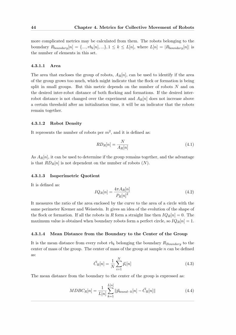
44 Chapter 4. Metrics for Collective Movement of Robots
more complicated metrics may be calculated from them. The robots belonging to theboundary Rboundary[n] = {..., rbk[n], ...}, 1 ≤ k ≤ L[n], where L[n] = |Rboundary[n]| isthe number of elements in this set.
4.3.1.1 Area
The area that encloses the group of robots, AR[n], can be used to identify if the areaof the group grows too much, which might indicate that the flock or formation is beingsplit in small groups. But this metric depends on the number of robots N and onthe desired inter-robot distance of both flocking and formations. If the desired inter-robot distance is not changed over the experiment and AR[n] does not increase abovea certain threshold after an initialization time, it will be an indicator that the robotsremain together.
4.3.1.2 Robot Density
It represents the number of robots per m2, and it is defined as:
RDR[n] =N
AR[n](4.1)
As AR[n], it can be used to determine if the group remains together, and the advantageis that RDR[n] is not dependent on the number of robots (N).
4.3.1.3 Isoperimetric Quotient
It is defined as:
IQR[n] =4πAR[n]PR[n]2
(4.2)
It measures the ratio of the area enclosed by the curve to the area of a circle with thesame perimeter Kremer and Weisstein. It gives an idea of the evolution of the shape ofthe flock or formation. If all the robots in R form a straight line then IQR[n] = 0. Themaximum value is obtained when boundary robots form a perfect circle, so IQR[n] = 1.
4.3.1.4 Mean Distance from the Boundary to the Center of the Group
It is the mean distance from every robot rbk belonging the boundary RBoundary to thecenter of mass of the group. The center of mass of the group at sample n can be definedas:
~CR[n] =1N
N∑
i=1
~pi[n] (4.3)
The mean distance from the boundary to the center of the group is expressed as:
MDBCR[n] =1
L[n]
L[n]∑
k=1
‖~pbound−k[n]− ~CR[n]‖ (4.4)

4.3. Metrics 45
where pbound−k is the position of robot rbk belonging to RBoundary. This metricrepresents a measure of the spatial size of the group of robots.
The metrics in this section are in general useful to identify some properties andbehaviors of the tested algorithms, but they cannot be used to compare quantitativelydifferent experiments.
4.3.2 Movement
This subset pretends to characterize the movement and trajectory of the group ofrobots.
4.3.2.1 Group Velocity
It is the velocity of the center of mass of the group.
~GV R[n] =~CR[n]− ~CR[n− 1]
T(4.5)
4.3.2.2 Average Group Speed
It is the average speed over the whole experiment of the center of mass of the group.
AGSR =1M
M∑
n=1
‖ ~V GR[n]‖ (4.6)
4.3.2.3 Length of the Trajectory
It is the length of the trajectory followed by the center of mass of the group.
LTR =M∑
n=2
(‖~CR[n]− ~CR[n− 1]‖) (4.7)
~GV R[n] and more specifically its magnitude (GSR[n]) can be plotted over the timeto get an idea of the evolution of the experiment. AGSR can be used to compare thequality of different algorithms, the higher average speed the better. LTR it is used tocalculate other metrics.
4.3.3 Quality
This subset of metrics measures the quality of the algorithms of flocking and formationof robots in terms of error in the positioning and the heading. Some of them can beonly used in formations while others are recommended for certain flocking or latticealgorithms. They can be used to compare the different algorithms in terms of errorpositioning and error orientation of their members.

46 Chapter 4. Metrics for Collective Movement of Robots
4.3.3.1 Mean Position Error
This metric is specific to formations of robots, where robots have pre-defined positionsto occupy. These positions can be defined with respect to the local frame of a leaderrobot. We impose that robot r1 is the leader robot. The desired positions of theneighboring robots referred to the leader frame are {..., ~pdes−i, ...}, 1 ≤ i ≤ N , where~pdes−l = (xdes−l, ydes−l). These positions are translated to the global reference frame,~pdes−glob−i = (xdes−glob−i, ydes−glob−i) where:
xdes−glob−i = x1 + xdes−i cos(θ1)− ydes−i sin(θ1) (4.8)
ydes−glob−i = y1 + xdes−i sin(θ1) + ydes−i cos(θ1) (4.9)
Taking into account this definitions the mean position error (averaged over the differentrobots) can be defined as:
MPER[n] =1N
N∑
i=1
‖~pdes−glob−i[n]− ~pi[n]‖ (4.10)
The desired pre-defined positions of the robots could also be defined with respect toa frame placed in the center of mass of the formation and with heading equal to themean global heading of all the robots.
MPER[n] can be averaged over the time duration of an experiment or severalexperiments to get a unique value and be able to compare how good different algorithmsare with respect to the positioning of the robots in the formation. The average ofMPER[n] over time is:
AMPER =1M
M∑
n=1
MPER[n] (4.11)
4.3.3.2 Mean Distance Error
There exist certain types of formations in which robots form triangular lattice patterns,maintaining a certain inter-robot distance to their closest neighboring robots. Someflocking algorithms also create these triangular lattice. In these kind of formations andflocks the inter-robot distance error averaged over the different robots and neighborscan be calculated in order to get a value of how well positioned the robots are, insteadof calculating MPER[n].
In order to calculate the mean distance error MDER, neighbors at a distance <
factor ∗ desiredInterRobotDistance(dd) will be considered to compute the distanceerror. For a robot ri its neighbors will be those belonging to Ni,δ for a δ = factor ∗ dd.factor can be set to 1.5.
MDER[n] =1N
N∑
i=1
1|Ni,δ[n]|
∑
rj∈Ni,δ[n]
|(‖~pj [n]− ~pi[n]‖)− dd| (4.12)

4.3. Metrics 47
4.3.3.3 Robot Density Error
It computes the difference between the RDR and an expected robot density RDDesired.In essence it can be used in flocking, when the algorithm tries to maintain robots at adesired inter-robot distance, and the flock is not too loose in its positioning. It can bealso used in robot formations. The RDDesired must be calculated for each experimentor algorithm depending on the desired inter-robot distance.
RDER[n] = RDR[n]−RDDesired (4.13)
This metric is used, as MDER[n], to show if robots maintain the desired inter-robotdistance or expected robot density.
4.3.3.4 Average Density Error
It is the average over time of the experiment of the RDER[n].
ARDER =1M
M∑
n=1
|RDER[n]| (4.14)
This value is useful to compare different algorithms. If algorithms with differentRDDesired must be compared a normalized NARDER value of ARDER might be used:
NARDER =ARDER
RDDesired(4.15)
4.3.3.5 Mean Orientation Error
This metric aims to measure how well oriented the robots are among the group.The error with respect a reference orientation is averaged over the different robots.This reference orientation θref can be the heading mean of all the robots or thedesired direction movement of the flock or formation in case it is known by thesystem that calculates the metrics. The heading mean can be calculated as follows:HMR = arg(
∑Ni=1 ~uθi), where ~uθi is a vector of magnitude 1 and direction θi. The
mean orientation error is:
MOER[n] =1N
N∑
i=1
|θi[n]− θref [n]| (4.16)
If robot orientations are equally spaced then∑N
i=1 ~uθi = ~0, so HMR will beundetermined, but in this case MOER[n] = π
2 , independently of θref .
4.3.3.6 Polarization
This metric is similar to MOER and also aims to measure how well oriented the robotsare. Polarization (Gutierrez et al., 2009) PoR of a group of robots R is defined using theangular nearest neighbor. For a robot ri, the corresponding angular nearest neighbourrann is defined so that θrirann , the relative orientation of rann with respect to ri is
48 Chapter 4. Metrics for Collective Movement of Robots
as small as possible: θrirann = min(θrirj ), ∀rj 6= ri ∈ R. We denote θann(ri, ξ[n])the relative orientation of the angular nearest neighbour of the robot ri. The formaldefinition of polarization is defined as follows:
PoR[n] =N∑
i=1
θann(ri, ξ[n]) (4.17)
If all robots are aligned, then PoR = 0. Conversely, if headings are evenly distributed,PoR = 2π. Lastly, if headings are random, i.e. drawn from a uniform distribution,then PoR = π in average. Meaningful comparisons among different group sizes arepossible since the average value of PoR is not affected by the number of robots in R.
4.3.3.7 Percentage of Time in Formation
This metric also represents a measure on how well positioned robots are in the formationduring an experiment. We can define the function Is in Formation to determine if thegroup is in formation taking into account the MPER:
IIF (R)[n] =
{1 if MPER[n] < e
0 if MPER[n] ≥ e(4.18)
where e is a certain arbitrary threshold. Then percentage of time in formation can becalculated as:
PTFR =∑M
n=1 IIF (R)[n]M
∗ 100 (4.19)
4.3.3.8 Time to Be In Formation
This metric calculates the time it takes the group of robots to reach MPER(t) < e,where is a certain arbitrary error threshold, as in the case of PTFR. It can be usedto measure how long it takes an algorithm to create a formation, but also to calculateother metrics like AGSR, average over time of PoR, and AMPER, not from t = 0 butfrom time to be in formation t = tIF .
4.3.4 Efficiency and Cost
The metrics of this subset try to measure the efficiency in terms of path followed by therobots and energy consumption. They are useful both to characterize the algorithmsand to compare them.
4.3.4.1 Path Length Ratio
It is the ratio between path length followed by the center of mass of the group andstraight line distance from the initial to the ending point.
PLRR =LTR
‖~CR[0]− ~CR[M ]‖(4.20)

4.3. Metrics 49
In case of absence of obstacles the interpretation is straight forward and the minimumvalue PLRR = 1 means an optimal movement of the flock or formation. When obstaclesare present it is necessary to compare between different algorithms or reformulate themetric to compute the ratio between the followed path length and the minimum possiblepath from starting point to ending point.
4.3.4.2 Single Robot Path Length Ratio
It is a similar metric to PLRR, but instead of using the path length of the center ofmass to calculate the ratio, the average of the path lengths of every robot is used.
SRPLRR =1N
∑Ni=1
(∑Mn=2(‖pi[n]− pi[n− 1]‖)
)
‖~CR[0]− ~CR[M ]‖(4.21)
4.3.4.3 Ratio Energy Consumption Distance Travelled
It is the ratio between the average of the energy consumption ECi in the experimentover the different robots and the straight line distance from the initial to the endingpoint.
RECDTR =1N
∑Ni=1 ECi
‖~CR[0]− ~CR[M ]‖(4.22)
In order to compute this metric it is also necessary to measure and report the energythat every robot uses during the experiment, which makes this metric more difficult touse.
4.3.5 Grouping
In collective movement of robots the group of robots R can split in several subgroups Rk,due to fails in the algorithm or on purpose in order to overcome an obstacle or just todivide and explore more efficiently the environment. The splitting in several subgroupsmust be detected in order to compute other metrics. For instance the trajectoriesfollowed by two split subgroups R1 and R2 must be calculated in a separated way usingthe centers of mass of of the different groups ~CR1 and ~CR2 and not the center of massof the complete group ~CR.
The different subgroups {..., Rk[n], ...}, 1 ≤ k ≤ K[n] can be calculated using theconnectivity properties of of G[n], where K[n] is the number of subgroups at sample n.If G[n] is is connected then R1[n] = R and there exists just one subgroup (K[n] = 1).Otherwise in order to determine the different subgroups Rk and their members ri theconnected sub-graphs of G[n] must be identified. A possible algorithm to do it is thefollowing:
S = R
i = 0
WHILE S is not empty
i = i+1
50 Chapter 4. Metrics for Collective Movement of Robots
rs = a robot in S
Ri = Ri + {rs}
S = S - {rs}
FOR each robot raux in S
IF there is path from rs to raux
S = S - {raux}
Ri = Ri + {raux}
ENDIF
ENDFOR
ENDWHILE
where R is the group of robots R, the operation Ri = Ri + {rs} adds the robot rs tothe subgroup Ri and S = S - {rs} removes the robot rs from the set S.
4.3.5.1 Number of Subgroups
It is the number of subgroups in which the whole group R is split.
NSR[n] = K[n] (4.23)
4.3.5.2 Size of a Subgroup
It is the number of robots that belong to a certain subgroup Rk.
SRk[n] = |Rk| (4.24)
If SRk[n] = N then Rk[n] = R. If SRk
[n] = 1, then the only robot belonging to thesubgroup Rk is isolated.
4.3.6 Success
These metrics measure the success of the algorithm in terms of robot failures andnumber of robots arriving together to the end. It can be used to compare the robustnessof different algorithms.
4.3.6.1 Ratio of Lost Robots
This metric is used to measure the number of robots that have lost the main subgroup.If we define the main subgroup Rm as the subgroup with maximum number of robotsthen:
RLRR[n] =N − |Rm[n]|
N(4.25)
An interesting value is the value at the end of the experiment RLRR[M ].
4.3. Metrics 51
4.3.6.2 Ratio of Not Working Robots
There are many ways to determine if a robot is not working any more. One of themcould be to determine if the robot is not moving for a while, but also robots couldidentify themselves as not working to report afterwards their state to the system incharge of calculating this metric. If NWR[n] is the number of not working robots atsample n, then:
RNWRR[n] =NWR[n]
N(4.26)
4.3.7 Security
The metric defined in this subset measures the security of the flock, in terms of distanceto obstacles.
4.3.7.1 Percentage of Time Group of Robots is Too Close to Obstacles
Distance to obstacles can be recorded using the in-built sensors of robots and couplingit with the information from the overhead camera. It might also be retrieved directlyfrom the tracking system by placing landmarks on top of the obstacles, in the case ofvery structured laboratory environments. We define the function TCR[n] whose resultis 1 if the group is too close to any obstacle and 0 otherwise:
TCR[n] =
{0 if ∀ri ∈ R,∀ol, ‖pi − pol
‖ > sd
1 otherwise(4.27)
where polis the position of all the points in the environment that describe the
boundaries of obstacles, and ol the obstacles in the environment. sd is the securitydistance that the group of robots must maintain with obstacles. Then,
PTTCOR[n] =∑M
n=1 TCR[n]N
∗ 100 (4.28)
4.3.8 Other
4.3.8.1 Mean Number of Neighboring Robots
This metric calculates the mean number of neighboring robots over the robots in R,showing how connected G[n] is.
MNNRR[n] =1N
N∑
i=1
|Ni,δ[n]| (4.29)
4.3.9 Higher Order Comparisons
Different types of comparisons can be done using two or more of the above describedmetrics. For instance in order to measure the scalability of the algorithms withincreasing number of robots, the variation of metrics like AGSR, AMPER, and ARDER
can be measured and plotted for different values of N . If AGSR does not decrease and
52 Chapter 4. Metrics for Collective Movement of Robots
the errors AMPER and ARDER do not increase with N increasing it will indicate thatthe algorithm is scalable.
In order to see how the error in positioning may affect the group speed and seeif there exist a correlation between both metrics, values of GSR[n] and RDER[n] fordifferent time steps n can be plotted in a graph using GSR and RDER as variables ofthe coordinate axes.
4.4 Conclusions
Several metrics for collective movement of robots have been defined and brieflydiscussed. Some of them are useful just to characterize the algorithms while otherscan be used to compare their performance. Some of the metrics depend on arbitraryparameters which could make the comparison between different algorithms difficult.
As it has been previously stated, in order to be able to compare different algorithms,it is necessary not only to have a set of metrics but to share a common set ofenvironments with obstacles and places that groups of robots must reach. This must bedone both in simulation and in the real world, defining simple laboratory environmentsthat can be easily reproduced.

Chapter 5
Distributed Orientation
Agreement in a Group of Robots
If we are facing in the right direction, all we have to do is keep on walking.
Buddhist Proverb
5.1 Introduction
A new method for a set of robots to agree in a distributed way on a common referenceorientation is presented, explained and analyzed in this chapter. Robots share andmaintain a common heading that is not related to any global reference and it is just aresult of their initial reference values. They do not make use of any global informationor compasses, the reference orientation is just computed by using a relative positioningsystem and wireless communications among neighboring robots. Sharing a commonreference orientation involves agreement on the directions and orientations of bothaxes of a coordinate system, but it does not imply agreement on the origin.
Sharing a common reference orientation can be quite useful in many collectivemovement algorithms. The first work on flocking (Reynolds, 1987), described in moredetail in Chapter 3, makes use of local rules between neighboring robots, forcing themto match their velocities. This implies that each agent must know the relative headingof its nearby mates, so having a common reference orientation can be useful. If robotsshare a common reference they can exchange their relative headings. This can be alsohelpful in many other flocking and formation algorithms (Carling et al., 2003; Chuanget al., 2007; Navarro et al., 2008, 2009), which require that the relative heading toneighboring robots is known. In addition, some formation architectures need of acommon reference orientation (Martinson and Payton, 2005; Lee and Chong, 2006).The proposed method of this chapter is used in the framework for collective movementdescribed in Chapter 6.
One of the most straight forward solutions in robotics, in order to share a referenceorientation, is to use magnetic compasses. As stated in Borenstein et al. (1996), themagnetic field of the earth can not be well measured near power lines or steel structures
54 Chapter 5. Distributed Orientation Agreement in a Group of Robots
due to their influence. In Ojeda and Borenstein (2000), a study of the sources of errorin a specific compass is made, concluding that some of them like vibration can onlybe partially filtered, while others like external interferences from the robot and otherelectromagnetic sources are more difficult to cope with. These drawbacks, togetherwith the need of providing every robot with a compass, is a reason for designing andimplementing the algorithm proposed in this chapter. On the other hand, in Turgutet al. (2008) and in Celikkanat et al. (2009), a group of robots is equipped withon-board magnetic compasses used to make robots flock. They assume that in thepresence of external interferences the sensed north remains approximately the samewithin neighboring robots. According to them, the measures are quite robust, even inindoor environments with metal objects.
In Navarro et al. (2008), robots move in a vertical plane, which allows robots to usegravity as a global orientation reference. They use their built-in 3-axes accelerometersto compute their heading with respect to gravity.
A method for agreement on a common orientation without the use of any globallandmark or compasses is described in Lee and Chong (2006). It starts identifying twopoints in the plane that indicate the reference heading. The first point is the centerof mass of the positions of all the robots in the group, while the second point is theposition of the most far away robot. This implies that in principle every robot should beaware of the relative positions of every robot in the group, which makes the algorithmnot scalable with increasing number of robots. In addition, it assumes perfect readingsin the location of nearby robots, and this is never the case in real robotic systems. Tworobots could identify different robots as the reference robot, resulting in no orientationagreement. So this method is not useful in real environments, and specially in swarmrobotic systems. Another method for agreement on the coordinate axes direction isexplained in Flocchini et al. (2008). It builds the reference axis while moving therobots to create a desired pattern, which is the principal aim of the algorithm.
The rest of this chapter is organized as follows. Section 5.2 explains the consensusproblem and its relationship with the proposed algorithm. The proposed algorithmis described, analyzed and commented in Section 5.3, while its test experiments andresults in simulation are presented in Section 5.4, and for real robots in Section 5.5.Conclusions are discussed in Section 5.6, while future lines of work are stated inSection 5.7.
5.2 Consensus Problems
Consensus problems are commonly referred to in the literature as those in which a setof inter-communicated agents must agree on the value of a variable. In our case wewant robots to agree on a reference direction. The resulting value in these problemsis sometimes the average of all the initial values in each agent, but depending on theapplication it can be the result of some other function.
The averaging problem serves as inspiration for our agreement on the angle ofreference, with the major difference that in our case we need to average angles, and

5.3. Method 55
angle values are cyclic since 2π is equivalent to 0. The averaging problem is explainedin Denantes (2007) as follows. Each agent i (or robot in our case) must update itsestimate vi[n] at each time step. The update operation is a linear combination of thecurrent estimation and the estimation of its neighbors:
vi[n + 1] = wii[n]vi[n] +∑
j∈Niwij [n]vj [n] i = 1...N (5.1)
where wij are the weighting factors that are defined depending on the algorithm, andNi represents the set of neighbors of agent i. The aim of these algorithms is to computethe average:
v =1N
N∑
i=1
vi[0] (5.2)
The convergence of these averaging algorithms and its conditions are explained andproved both in Denantes (2007) and Xiao and Boyd (2003).
The problem of the averaging agreement in asynchronous systems and a solutionbased on an exchange message protocol is explained in Mehyar et al. (2005). It is aquite conservative solution but serves to maintain
∑Ni=1 vi[n] the same for every time
step.Olfati-Saber and Murray (2003) present the problem of introducing time-delays
when using consensus protocols. Several methods are used to analyze its convergence.Simulations results are presented for few cases.
Some of the applications of the consensus problem include: sensor and informationfusion (Talebi et al., 2006; Xiao et al., 2005); coordination of groups of robots (Olfati-Saber, 2006; Tanner et al., 2003a,b; Jadbabaie et al., 2003), in the same way as theaim of this Thesis; and coordinated decision making (Bauso et al., 2003; Alanyali et al.,2004). A review of consensus problem on cooperation of robots is presented in Renet al. (2007).
5.3 Method
The aim of the proposed method is to make a group of robots agree on a referenceorientation without the use of any external reference, compass or global positioningsystem. The sensoring and communication systems used by the robots in this methodare:
• Encoders or any other odometry system to keep track of the robot’s headingchanges;
• A wireless communication system to send and receive messages with neighboringrobots;
• A relative positioning system, similar to Pugh et al. (2009), explained inSection A.1.1, which allows each robot to determine the relative position (distanceand bearing) of neighboring robots within a certain range, and their identificationnumbers.

56 Chapter 5. Distributed Orientation Agreement in a Group of Robots
The method works as follows. Every robot has an initial estimate of the referenceorientation which represents the direction the group of robots must agree on. Robotsexchange this estimate among them and apply a consensus algorithm in order to agree.This direction is expressed on each robot relative to its own coordinate system, soeach pair of neighboring robots that exchanges their estimates must know their relativeheadings. This is performed by using a relative positioning system and exchangingwireless messages. In addition, the rotation of the robot must be taken into accountby reading the robot encoders and modifying its reference orientation estimate. Thebasic steps of the algorithm, executed cyclically, are the following:
1. Reading the bearings to see neighboring robots from the relative positioningsystem, and saving the values together with a timestamp.
2. Reading the received wireless messages from every neighboring robots, whichcontain information about the reference orientation estimate of each neighboringrobot and the own bearing seen by the neighboring robot.
3. Transforming the neighboring reference orientation estimates to the own coordi-nate system using the previously received information.
4. Applying the consensus algorithm to update the reference orientation estimateusing the neighbor’s estimates.
5. Correcting the estimate, to take into account the changes in robot’s heading,using the odometry readings.
6. Creating and sending wireless messages to neighboring robots. These messagesinclude the reference orientation estimate and the bearing to the neighbor robotalong with the timestamp specifying the moment when the robot was observed.
In order to make each robot know the relative heading of their neighboring robotsand compute the new reference orientation estimate, they share and store the followinginformation. Robot ri reads the relative position and identification number of eachof its neighboring robots rj , storing the relative bearing to the neighbor (θi,j), theneighbor’s identification number (IDj), and the time (ti), according to the timing ofrobot ri when the relative position was estimated. Afterwards each robot ri sends toeach one of its neighboring robots rj the following information: its own identificationnumber (IDi); the bearing (θi,j(ti)) of robot rj at time ti; the time stamp when rj wasseen (ti); and lastly its current estimate of the orientation reference θreference,i.
If we consider that robots are not moving, the orientation reference (θreference,i) ofrobot ri expressed in the coordinate system of robot rj (θreference,i,j), can be calculatedby robot rj without considering the timing, as follows:
θreference,i,j = θj,i − θi,j + π + θreference,i (5.3)
In Figure 5.1 a schematic with the angles involved in this operation is outlined.

5.3. Method 57
Figure 5.1: Angles involved in the calculation of θreference,i,j
In principle robots move and messages suffer from delays so for robot rj to calculateθreference,i,j applying Equation 5.3 needs to use θj,i and θi,j , which correspond to exactlythe same moment. In principle it is considered that robots’ clocks are synchronized.
Each cycle, robot rj reads its relative position to neighboring robot ri and storesthis information together with the time stamp. Robot ri does the same, to later sendthis information via wireless to robot rj . When robot rj receives θi,j(ti) from robot ri ithas suffered a delay, so it has to retrieve the value of θj,i(tj) corresponding to the sameinstant ti = tj . If Equation 5.3 is applied with these values the resulting θreference,i,j
will be for the time tj , which, in principle, due to the delays, is not the current time.So it is important to correct it using the change of heading ∆odometry(t′j , tj) of robotrj , from tj to the moment t′j , when the θreference,j was estimated last. Then thesevalues will be the inputs to the consensus algorithm. The following equation takesthese details into account:
θreference,i,j(t′j) = θj,i(tj)− θi,j(ti) + π + θreference,i −∆odometry(t′j , tj) (5.4)
Robot rj needs to get θj,i(tj) from its stored values. Since probably the value will notbe stored for that exact moment, the robot will interpolate from the two samples withtiming values around tj . The same applies for the odometry ∆odometry(t′j , tj).
Robot rj (and each one of the robots in the group) will calculate θreference,i,j(t′j)for every neighbor ri ∈ Nj , from which receives a wireless message containing θi,j(ti)and ti. The topology of the associated communication graph changes in principle withthe movement of the robots and the failures of the communication systems, so theneighbors of each robot and the number of them will change over time.
Once the reference orientation of neighboring robots is translated to the coordinatesystem of the robot, a consensus algorithm using these values and its own estimate canbe applied to compute the new estimate. Two different algorithms for this purposeare described in Section 5.3.1 and Section 5.3.2. This can be summarized in the nextequation:
θreference,j(t′j) = f(θreference,j(t′j), ..., θreference,i,j(t′j), ...) ∀i ∈ Nj (5.5)

58 Chapter 5. Distributed Orientation Agreement in a Group of Robots
One of the last steps in the cycle of the algorithm is to update θreference,j with theodometry for the current time t′′j :
θreference,j(t′′j ) = θreference,j(t′j)−∆odometry(t′′j , t′j) (5.6)
Lastly, wireless messages are sent to the neighboring robots including the updatedvalue θreference,j(t′′j ).
5.3.1 Consensus Algorithm A
In this section the Consensus Algorithm A (CAA) is described. This algorithm isexecuted by every robot ri in order to agree on the common reference orientationusing as inputs the reference orientations (θreference,j,i) of neighboring robots rj ∈Ni transposed to the coordinates of ri, and its own reference orientation estimate(θreference,i).
It is implemented in a similar way as the consensus averaging solution explained inSection 5.2 and described by Equation 5.2. The main difference is that here an averageover angles must be done, and due to the circular property of angles (2π equivalentto 0) they can not be directly weighted and added. Instead, angles are convertedto unit vectors with the direction of the angles. If we denote ~vreference,i as the unitvector of angle θreference,i, and ~vreference,j,i as the unit vector of angle θreference,j,i, thenEquation 5.2can be rewritten as follows:
~vreference,i[n + 1] = wii[n]~vreference,i[n] +∑
j∈Ni
wij [n]~vreference,j,i[n] (5.7)
The new reference estimate is calculated by obtaining the angle of ~vreference,i[n + 1]:
θreference,i[n + 1] = arg(~vreference,i[n + 1]) (5.8)
The weighting parameters wij will all be set to a configuring parameter α, whilewii = 1−∑
j∈Niwij = 1−∑
Niα, where Ni is the number of neighbors of ri. If wii < α,
then wii = wij = 1Ni+1 . This will depend on the number of neighbors that a robot ri
will have at a certain moment. The range of α must be 0 < α ≤ 0.5. The value ofα is going to determine the velocity of convergence and its accuracy as explained inSection 5.4.
If we were working with real numbers and wanted to agree on using the average,the convergence of these algorithms can be demonstrated under certain conditions asoutlined in Section 5.2. But in this case we want to agree on an angle, and angles havethe property of being cyclical in their values, since 2π is equivalent to 0. In Jadbabaieet al. (2003), the convergence is demonstrated working without taking into account thecyclical property. The resulting average of θ1 = 0 and θ2 = 2π would be π and not0. In their case it can be done because the agents in this algorithm share a commonglobal coordinate system, but this is not the case of the present method.

5.3. Method 59
Here we present an example in which our algorithm does not converge. As will beseen in Section 5.4, this is a very similar situation to what has been seen in some ofthe obtained results. In Figure 5.2, four robots are shown, each of them having twoneighboring robots, and with evenly distributed reference orientations indicated by thevectors. If we consider no communication loses, perfect synchronization in the robots’clocks, and that robots update their estimates synchronously, then given the initialreference orientations, CAA will not converge. For robot r1 we have:
~vreference,1[n + 1] =
(1− 2α) ∗ ~vreference,1[n] + α ∗ ~vreference,4,1[n] + α ∗ ~vreference,2,1[n] = (5.9)
(1− 2α) ∗ ~vreference,1[n]
since vreference,2,1 and vreference,4,1 are cancelled with each other. Then, the resultingθreference,1 will be the same as the initial one. The same happens for the four robots,so they will never agree on a common reference orientation.
Figure 5.2: An initial condition in which CAA does not converge.
Next section describes a modification of CAA, that intuitively overcomes theproblem described in this previous example.
5.3.2 Consensus Algorithm B
Consensus Algorithm B (CAB) is a modification of CAA, to overcome the convergenceproblem experienced under certain topology configurations. The basic idea behindCAB is that initially there exists a robot which imposes its orientation reference toits neighbors, in the next step its neighbors do the same, an so on, resulting in apropagation by flooding of the initial reference orientation of one of the robots.
In CAB robots maintain and exchange via wireless messages a variable about howconfident they are on their reference orientation estimate. Initially every robot has thisvariable set to zero, except one of the robots that will have it set to one. We will name
60 Chapter 5. Distributed Orientation Agreement in a Group of Robots
this robot seed robot. Confidence is used to estimate the new orientation reference,creating the propagation of the initial reference orientation of the seed robot. When arobot updates its orientation estimate it also updates its confidence setting it to themaximum of its own confidence and neighbors’ confidences. It can be summarized inthe following equations:
~vreference,i[n + 1] = ci[n]wii[n]~vreference,i[n] +∑
j∈Ni
cj [n]wij [n]~vreference,j,i[n] (5.10)
ci[n + 1] = max(ci[n], ..., cj [n], ...) ∀j ∈ Ni (5.11)
where ci is the confidence variable of robot ri and cj the confidence of neighbor rj .After the propagation of the reference orientation of the seed robot, every robot will
have a similar reference orientation, that will be slightly different due to the errorsintroduced by noise and lack of synchronicity. After that CAB will act basicallyas a distributed filter on the common reference orientation. We will not prove theconvergence of CAB here, but it wil be tested empirically. After the propagation everyrobot will practically agree on the reference orientation.
The example explained in CAA (Figure 5.2) will in this case converge to thereference orientation of the robot which will be labeled as seed robot.
5.4 Experiments in Simulation
In order to test the method described in this chapter, systematic experiments wereperformed both with real robots and in simulation. Simulated experiments and theirresults are the scope of this section, while real robot experiments are described inSection 5.5. Simulated experiments were run using Webots simulator, with a realisticmodel of the Khepera III robot. These systems are described in more detail inAppendix A.
We ran nine different sets of simulated experiments, each one composed of 30different experiments, with the same parameters but different random initial headingsof the robots. The sets are differentiated by:
• the α parameter of the consensus algorithm,
• the topology of the robots’ communication graph,
• the behavior of the robots,
• the presence or not of error in the synchronicity of the robots’ clocks,
• and the consensus algorithm chosen (CAA or CAB).
All the experiments were run using 49 robots, placed in one of the two communicationtopologies chosen: square lattice and ring. In the square lattice topology the 49 robotsare placed in seven rows and seven columns, inner robots having four neighbors andbordering robots two or three neighbors. A schematic of this topology with less robots
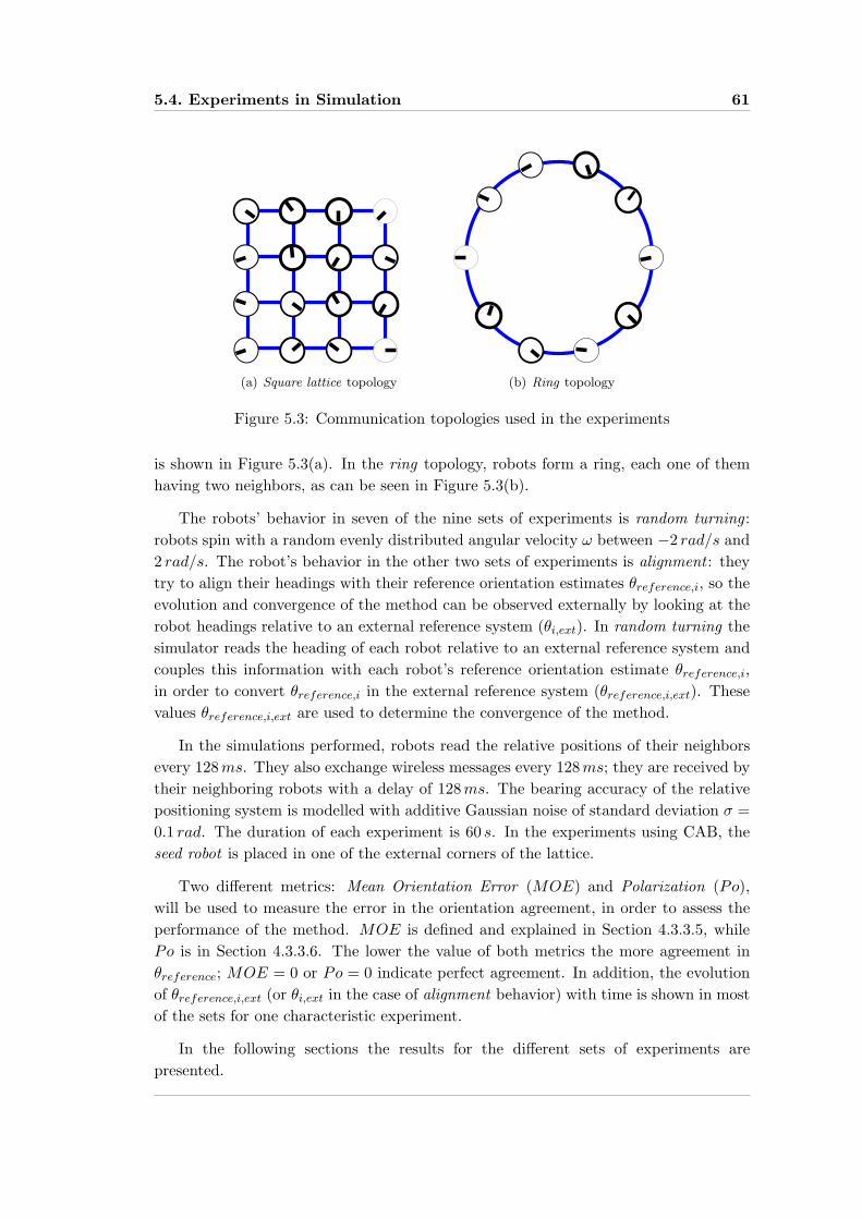
5.4. Experiments in Simulation 61
(a) Square lattice topology (b) Ring topology
Figure 5.3: Communication topologies used in the experiments
is shown in Figure 5.3(a). In the ring topology, robots form a ring, each one of themhaving two neighbors, as can be seen in Figure 5.3(b).
The robots’ behavior in seven of the nine sets of experiments is random turning :robots spin with a random evenly distributed angular velocity ω between −2 rad/s and2 rad/s. The robot’s behavior in the other two sets of experiments is alignment : theytry to align their headings with their reference orientation estimates θreference,i, so theevolution and convergence of the method can be observed externally by looking at therobot headings relative to an external reference system (θi,ext). In random turning thesimulator reads the heading of each robot relative to an external reference system andcouples this information with each robot’s reference orientation estimate θreference,i,in order to convert θreference,i in the external reference system (θreference,i,ext). Thesevalues θreference,i,ext are used to determine the convergence of the method.
In the simulations performed, robots read the relative positions of their neighborsevery 128ms. They also exchange wireless messages every 128ms; they are received bytheir neighboring robots with a delay of 128ms. The bearing accuracy of the relativepositioning system is modelled with additive Gaussian noise of standard deviation σ =0.1 rad. The duration of each experiment is 60 s. In the experiments using CAB, theseed robot is placed in one of the external corners of the lattice.
Two different metrics: Mean Orientation Error (MOE) and Polarization (Po),will be used to measure the error in the orientation agreement, in order to assess theperformance of the method. MOE is defined and explained in Section 4.3.3.5, whilePo is in Section 4.3.3.6. The lower the value of both metrics the more agreement inθreference; MOE = 0 or Po = 0 indicate perfect agreement. In addition, the evolutionof θreference,i,ext (or θi,ext in the case of alignment behavior) with time is shown in mostof the sets for one characteristic experiment.
In the following sections the results for the different sets of experiments arepresented.
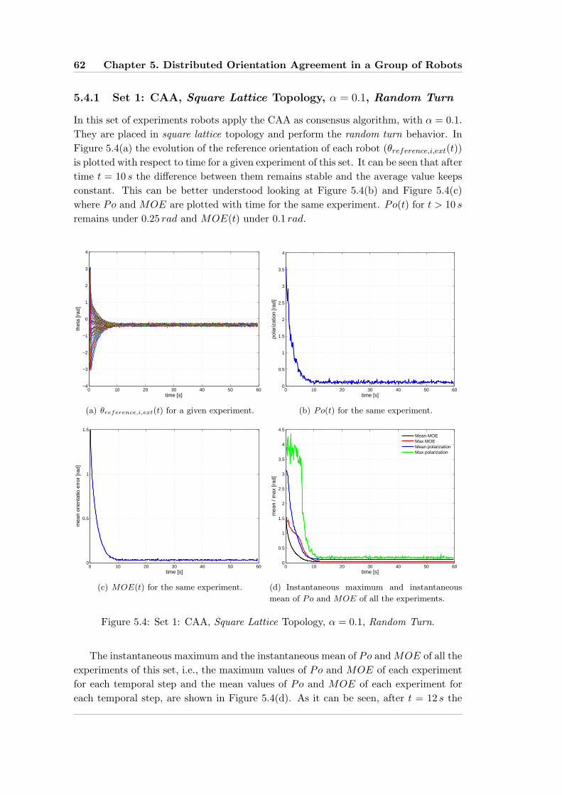
62 Chapter 5. Distributed Orientation Agreement in a Group of Robots
5.4.1 Set 1: CAA, Square Lattice Topology, α = 0.1, Random Turn
In this set of experiments robots apply the CAA as consensus algorithm, with α = 0.1.They are placed in square lattice topology and perform the random turn behavior. InFigure 5.4(a) the evolution of the reference orientation of each robot (θreference,i,ext(t))is plotted with respect to time for a given experiment of this set. It can be seen that aftertime t = 10 s the difference between them remains stable and the average value keepsconstant. This can be better understood looking at Figure 5.4(b) and Figure 5.4(c)where Po and MOE are plotted with time for the same experiment. Po(t) for t > 10 s
remains under 0.25 rad and MOE(t) under 0.1 rad.
0 10 20 30 40 50 60−4
−3
−2
−1
0
1
2
3
4
time [s]
thet
a [r
ad]
(a) θreference,i,ext(t) for a given experiment.
0 10 20 30 40 50 600
0.5
1
1.5
2
2.5
3
3.5
4
time [s]
pola
rizat
ion
[rad
]
(b) Po(t) for the same experiment.
0 10 20 30 40 50 600
0.5
1
1.5
time [s]
mea
n or
ient
atio
err
or [r
ad]
(c) MOE(t) for the same experiment.
0 10 20 30 40 50 600
0.5
1
1.5
2
2.5
3
3.5
4
4.5
time [s]
mea
n / m
ax [r
ad]
Mean MOEMax MOEMean polarizationMax polarization
(d) Instantaneous maximum and instantaneous
mean of Po and MOE of all the experiments.
Figure 5.4: Set 1: CAA, Square Lattice Topology, α = 0.1, Random Turn.
The instantaneous maximum and the instantaneous mean of Po and MOE of all theexperiments of this set, i.e., the maximum values of Po and MOE of each experimentfor each temporal step and the mean values of Po and MOE of each experiment foreach temporal step, are shown in Figure 5.4(d). As it can be seen, after t = 12 s the
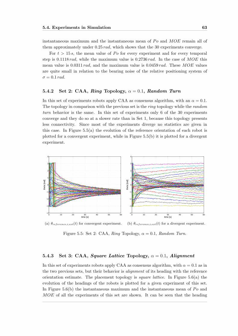
5.4. Experiments in Simulation 63
instantaneous maximum and the instantaneous mean of Po and MOE remain all ofthem approximately under 0.25 rad, which shows that the 30 experiments converge.
For t > 15 s, the mean value of Po for every experiment and for every temporalstep is 0.1118 rad, while the maximum value is 0.2736 rad. In the case of MOE thismean value is 0.0311 rad, and the maximum value is 0.0459 rad. These MOE valuesare quite small in relation to the bearing noise of the relative positioning system ofσ = 0.1 rad.
5.4.2 Set 2: CAA, Ring Topology, α = 0.1, Random Turn
In this set of experiments robots apply CAA as consensus algorithm, with an α = 0.1.The topology in comparison with the previous set is the ring topology while the randomturn behavior is the same. In this set of experiments only 6 of the 30 experimentsconverge and they do so at a slower rate than in Set 1, because this topology presentsless connectivity. Since most of the experiments diverge no statistics are given inthis case. In Figure 5.5(a) the evolution of the reference orientation of each robot isplotted for a convergent experiment, while in Figure 5.5(b) it is plotted for a divergentexperiment.
0 10 20 30 40 50 60−4
−3
−2
−1
0
1
2
3
4
time [s]
thet
a [r
ad]
(a) θreference,i,ext(t) for convergent experiment.
0 10 20 30 40 50 60−4
−3
−2
−1
0
1
2
3
4
time [s]
thet
a [r
ad]
(b) θreference,i,ext(t) for a divergent experiment.
Figure 5.5: Set 2: CAA, Ring Topology, α = 0.1, Random Turn.
5.4.3 Set 3: CAA, Square Lattice Topology, α = 0.1, Alignment
In this set of experiments robots apply CAA as consensus algorithm, with α = 0.1 as inthe two previous sets, but their behavior is alignment of its heading with the referenceorientation estimate. The placement topology is square lattice. In Figure 5.6(a) theevolution of the headings of the robots is plotted for a given experiment of this set.In Figure 5.6(b) the instantaneous maximum and the instantaneous mean of Po andMOE of all the experiments of this set are shown. It can be seen that the heading

64 Chapter 5. Distributed Orientation Agreement in a Group of Robots
agreement is better than in Set 1, this is because the alignment controller filters theorientation estimates θreference,i.
0 10 20 30 40 50 60−4
−3
−2
−1
0
1
2
3
4
time [s]
thet
a [r
ad]
(a) θi,ext(t) for a given experiment.
0 10 20 30 40 50 600
0.5
1
1.5
2
2.5
3
3.5
4
4.5
time [s]
mea
n / m
ax [r
ad]
Mean MOEMax MOEMean polarizationMax polarization
(b) Instantaneous maximum and instantaneous
mean of Po and MOE of all the experiments.
Figure 5.6: Set 3: CAA, Square Lattice Topology, α = 0.1, Alignment.
After t = 15 s the difference in the headings is very small. All the experimentsconverge. The mean of Po for every experiment and for every temporal step after t =15 s is 0.0420 rad, while the maximum of Po is 0.0997 rad. For MOE the correspondingvalues are 0.0115 rad for the mean and 0.0313 rad for the maximum. These values aresmaller than in Set 1.
5.4.4 Set 4: CAB, Square Lattice Topology, α = 0.1, Random Turn
This set of experiments uses the CAB for consensus, with α = 0.1. The communicationtopology is Square Lattice and the behavior Random Turn. The conditions are thenthe same as in Set 1, but applying CAB instead of CAA. Figure 5.7 shows theevolution of θreference,i,ext(t), Po(t), MOE(t), and the instantaneous maximum andthe instantaneous mean of Po and MOE. It can be seen that CAB converges fasterthan CAA with the same parameters. In the worst case for t > 2 s MOE and Po areunder 0.3 rad. This is due to the propagation of the θreference,i of the seed robot.
Mean of Po for every experiment and for every temporal step after t = 15 s is0.1119 rad, and the maximum is 0.2368 rad. For MOE the corresponding values are0.0310 rad for the mean and 0.0461 rad for the maximum.
5.4.5 Set 5: CAB, Square Lattice Topology, α = 0.01, Random Turn
This set is the same as Set 4 but with α = 0.01, so it uses CAB, the topology is SquareLattice and the behavior Random Turn. As it can be seen in Figure 5.8(a), where theorientation reference estimates of every robot in a given experiment are plotted, theconvergence is slower than in Set 4 (α = 0.1), but it reaches smaller differences between
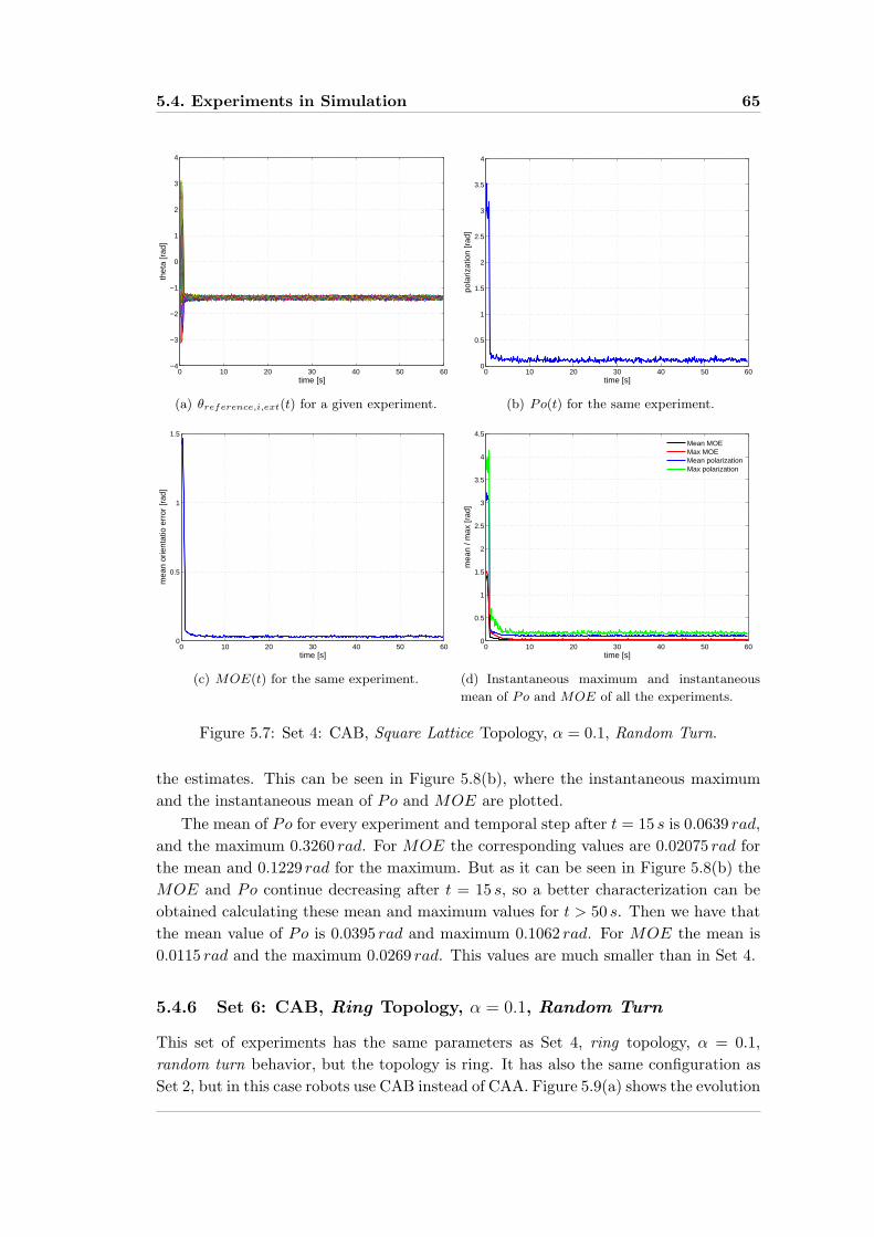
5.4. Experiments in Simulation 65
0 10 20 30 40 50 60−4
−3
−2
−1
0
1
2
3
4
time [s]
thet
a [r
ad]
(a) θreference,i,ext(t) for a given experiment.
0 10 20 30 40 50 600
0.5
1
1.5
2
2.5
3
3.5
4
time [s]
pola
rizat
ion
[rad
]
(b) Po(t) for the same experiment.
0 10 20 30 40 50 600
0.5
1
1.5
time [s]
mea
n or
ient
atio
err
or [r
ad]
(c) MOE(t) for the same experiment.
0 10 20 30 40 50 600
0.5
1
1.5
2
2.5
3
3.5
4
4.5
time [s]
mea
n / m
ax [r
ad]
Mean MOEMax MOEMean polarizationMax polarization
(d) Instantaneous maximum and instantaneous
mean of Po and MOE of all the experiments.
Figure 5.7: Set 4: CAB, Square Lattice Topology, α = 0.1, Random Turn.
the estimates. This can be seen in Figure 5.8(b), where the instantaneous maximumand the instantaneous mean of Po and MOE are plotted.
The mean of Po for every experiment and temporal step after t = 15 s is 0.0639 rad,and the maximum 0.3260 rad. For MOE the corresponding values are 0.02075 rad forthe mean and 0.1229 rad for the maximum. But as it can be seen in Figure 5.8(b) theMOE and Po continue decreasing after t = 15 s, so a better characterization can beobtained calculating these mean and maximum values for t > 50 s. Then we have thatthe mean value of Po is 0.0395 rad and maximum 0.1062 rad. For MOE the mean is0.0115 rad and the maximum 0.0269 rad. This values are much smaller than in Set 4.
5.4.6 Set 6: CAB, Ring Topology, α = 0.1, Random Turn
This set of experiments has the same parameters as Set 4, ring topology, α = 0.1,random turn behavior, but the topology is ring. It has also the same configuration asSet 2, but in this case robots use CAB instead of CAA. Figure 5.9(a) shows the evolution

66 Chapter 5. Distributed Orientation Agreement in a Group of Robots
0 10 20 30 40 50 60−4
−3
−2
−1
0
1
2
3
4
time [s]
thet
a [r
ad]
(a) θreference,i,ext(t) for a given experiment.
0 10 20 30 40 50 600
0.5
1
1.5
2
2.5
3
3.5
4
4.5
time [s]
mea
n / m
ax [r
ad]
Mean MOEMax MOEMean polarizationMax polarization
(b) Instantaneous maximum and instantaneous
mean of Po and MOE of all the experiments.
Figure 5.8: Set 5: CAB, Square Lattice Topology, α = 0.01, Random Turn.
of θreference,i,ext for a particular experiment. As it can be seen it converges, but moreslowly than in Set 4 (square lattice topology). In Figure 5.9(b) the instantaneousmaximum and the instantaneous mean of Po and MOE of all the experiments in theset are plotted. Comparing this figure to Figure 5.7 of Set 4, we can see that the suddensteep change in the mean Po and the mean MOE occurs later in Set 6. This is due tothe topology of Set 6, since the reference orientation propagates from the seed robot,jumping from two robots to other two different each step, so it takes longer to reachthe last robot than with the square lattice topology where robots are more connected.In addition, after this abrupt drop in MOE and Po they continue decreasing and int = 60 s these values are on average higher than in Set 4. It is again due to the lessconnected topology of Set 6.
0 10 20 30 40 50 60−4
−3
−2
−1
0
1
2
3
4
time [s]
thet
a [r
ad]
(a) θreference,i,ext(t) for a given experiment.
0 10 20 30 40 50 600
0.5
1
1.5
2
2.5
3
3.5
4
4.5
time [s]
mea
n / m
ax [r
ad]
Mean MOEMax MOEMean polarizationMax polarization
(b) Instantaneous maximum and instantaneous
mean of Po and MOE of all the experiments.
Figure 5.9: Set 6: CAB, Ring Topology, α = 0.1, Random Turn.
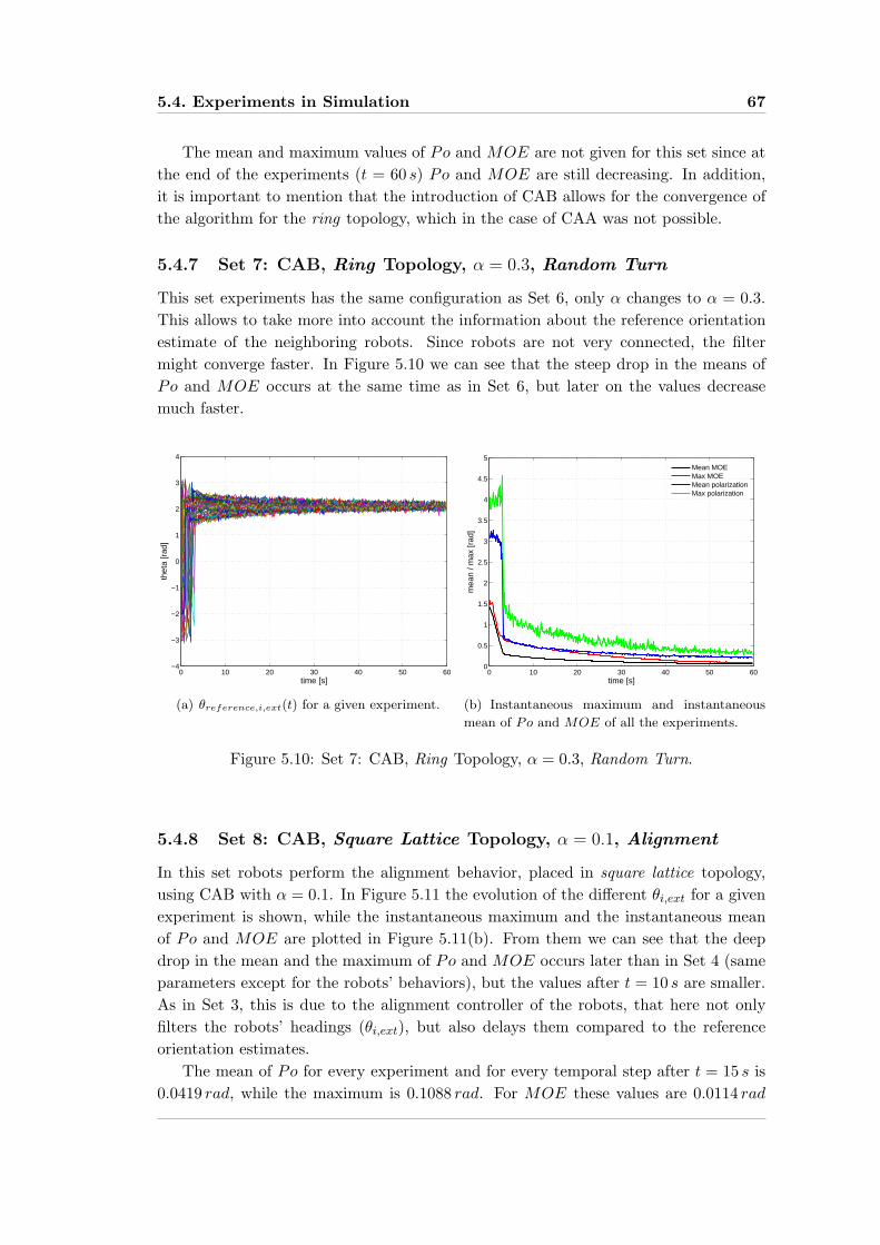
5.4. Experiments in Simulation 67
The mean and maximum values of Po and MOE are not given for this set since atthe end of the experiments (t = 60 s) Po and MOE are still decreasing. In addition,it is important to mention that the introduction of CAB allows for the convergence ofthe algorithm for the ring topology, which in the case of CAA was not possible.
5.4.7 Set 7: CAB, Ring Topology, α = 0.3, Random Turn
This set experiments has the same configuration as Set 6, only α changes to α = 0.3.This allows to take more into account the information about the reference orientationestimate of the neighboring robots. Since robots are not very connected, the filtermight converge faster. In Figure 5.10 we can see that the steep drop in the means ofPo and MOE occurs at the same time as in Set 6, but later on the values decreasemuch faster.
0 10 20 30 40 50 60−4
−3
−2
−1
0
1
2
3
4
time [s]
thet
a [r
ad]
(a) θreference,i,ext(t) for a given experiment.
0 10 20 30 40 50 600
0.5
1
1.5
2
2.5
3
3.5
4
4.5
5
time [s]
mea
n / m
ax [r
ad]
Mean MOEMax MOEMean polarizationMax polarization
(b) Instantaneous maximum and instantaneous
mean of Po and MOE of all the experiments.
Figure 5.10: Set 7: CAB, Ring Topology, α = 0.3, Random Turn.
5.4.8 Set 8: CAB, Square Lattice Topology, α = 0.1, Alignment
In this set robots perform the alignment behavior, placed in square lattice topology,using CAB with α = 0.1. In Figure 5.11 the evolution of the different θi,ext for a givenexperiment is shown, while the instantaneous maximum and the instantaneous meanof Po and MOE are plotted in Figure 5.11(b). From them we can see that the deepdrop in the mean and the maximum of Po and MOE occurs later than in Set 4 (sameparameters except for the robots’ behaviors), but the values after t = 10 s are smaller.As in Set 3, this is due to the alignment controller of the robots, that here not onlyfilters the robots’ headings (θi,ext), but also delays them compared to the referenceorientation estimates.
The mean of Po for every experiment and for every temporal step after t = 15 s is0.0419 rad, while the maximum is 0.1088 rad. For MOE these values are 0.0114 rad
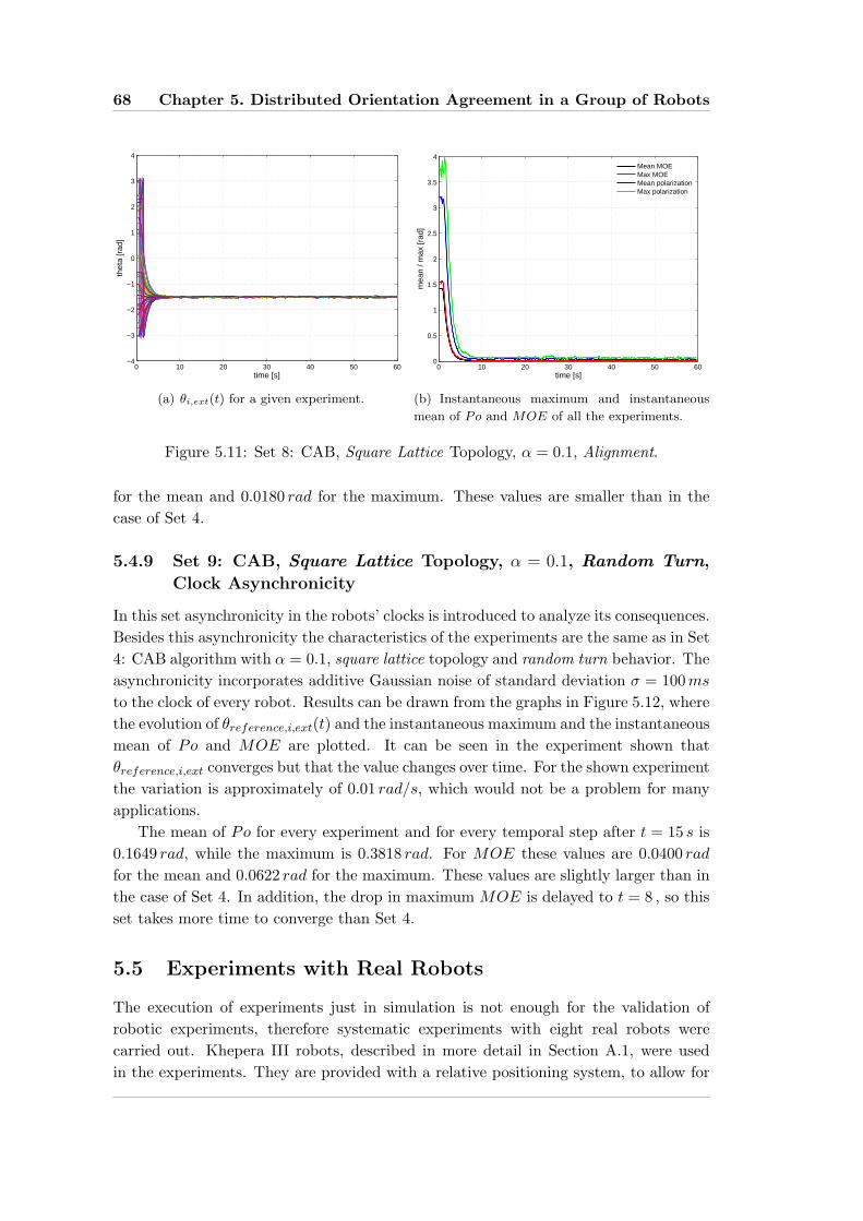
68 Chapter 5. Distributed Orientation Agreement in a Group of Robots
0 10 20 30 40 50 60−4
−3
−2
−1
0
1
2
3
4
time [s]
thet
a [r
ad]
(a) θi,ext(t) for a given experiment.
0 10 20 30 40 50 600
0.5
1
1.5
2
2.5
3
3.5
4
time [s]
mea
n / m
ax [r
ad]
Mean MOEMax MOEMean polarizationMax polarization
(b) Instantaneous maximum and instantaneous
mean of Po and MOE of all the experiments.
Figure 5.11: Set 8: CAB, Square Lattice Topology, α = 0.1, Alignment.
for the mean and 0.0180 rad for the maximum. These values are smaller than in thecase of Set 4.
5.4.9 Set 9: CAB, Square Lattice Topology, α = 0.1, Random Turn,
Clock Asynchronicity
In this set asynchronicity in the robots’ clocks is introduced to analyze its consequences.Besides this asynchronicity the characteristics of the experiments are the same as in Set4: CAB algorithm with α = 0.1, square lattice topology and random turn behavior. Theasynchronicity incorporates additive Gaussian noise of standard deviation σ = 100ms
to the clock of every robot. Results can be drawn from the graphs in Figure 5.12, wherethe evolution of θreference,i,ext(t) and the instantaneous maximum and the instantaneousmean of Po and MOE are plotted. It can be seen in the experiment shown thatθreference,i,ext converges but that the value changes over time. For the shown experimentthe variation is approximately of 0.01 rad/s, which would not be a problem for manyapplications.
The mean of Po for every experiment and for every temporal step after t = 15 s is0.1649 rad, while the maximum is 0.3818 rad. For MOE these values are 0.0400 rad
for the mean and 0.0622 rad for the maximum. These values are slightly larger than inthe case of Set 4. In addition, the drop in maximum MOE is delayed to t = 8 , so thisset takes more time to converge than Set 4.
5.5 Experiments with Real Robots
The execution of experiments just in simulation is not enough for the validation ofrobotic experiments, therefore systematic experiments with eight real robots werecarried out. Khepera III robots, described in more detail in Section A.1, were usedin the experiments. They are provided with a relative positioning system, to allow for

5.5. Experiments with Real Robots 69
0 10 20 30 40 50 60−4
−3
−2
−1
0
1
2
3
4
time [s]
thet
a [r
ad]
(a) θreference,i,ext(t) for a given experiment.
0 10 20 30 40 50 600
0.5
1
1.5
2
2.5
3
3.5
4
4.5
time [s]
mea
n / m
ax [r
ad]
Mean MOEMax MOEMean polarizationMax polarization
(b) Instantaneous maximum and instantaneous
mean of Po and MOE of all the experiments.
Figure 5.12: Set 9: CAB, Square Lattice Topology, α = 0.1, Random Turn.
the estimation of the relative position of nearby robots. This system is explained inmore detail in Section A.1.1.
Two different sets of experiments with real robots were run, each one composed of 20different experiments, with the same parameters but different random initial headingsof the robots. Both sets are only differentiated by the type of consensus algorithm used:CAA in one case and CAB in the other. The behavior of the robots is alignment, andso the evolution and convergence of the experiments can be determined externally bylooking at the robot headings. Other behaviors were not tested in the case of real robotssince there is no possibility of inner inspection of the robots’ states in a synchronizedmanner. Robots are placed to form a square lattice topology, consisting of two rowsof three robots and a third one of two robots, depicted in Figure 5.13 indicating thecommunication graph by the blue connection lines.
Figure 5.13: Communication topology of type square lattice used in the experimentswith real robots.
In simulation, robots perform a complete cycle of the algorithm in a fixed periodof time but in reality this period varies from cycle to cycle and robot to robot. Thisperiod was measured in several experiments and it was in most cases around 180ms.The duration of each experiment is 60 s, the same as in the simulation experiments. In
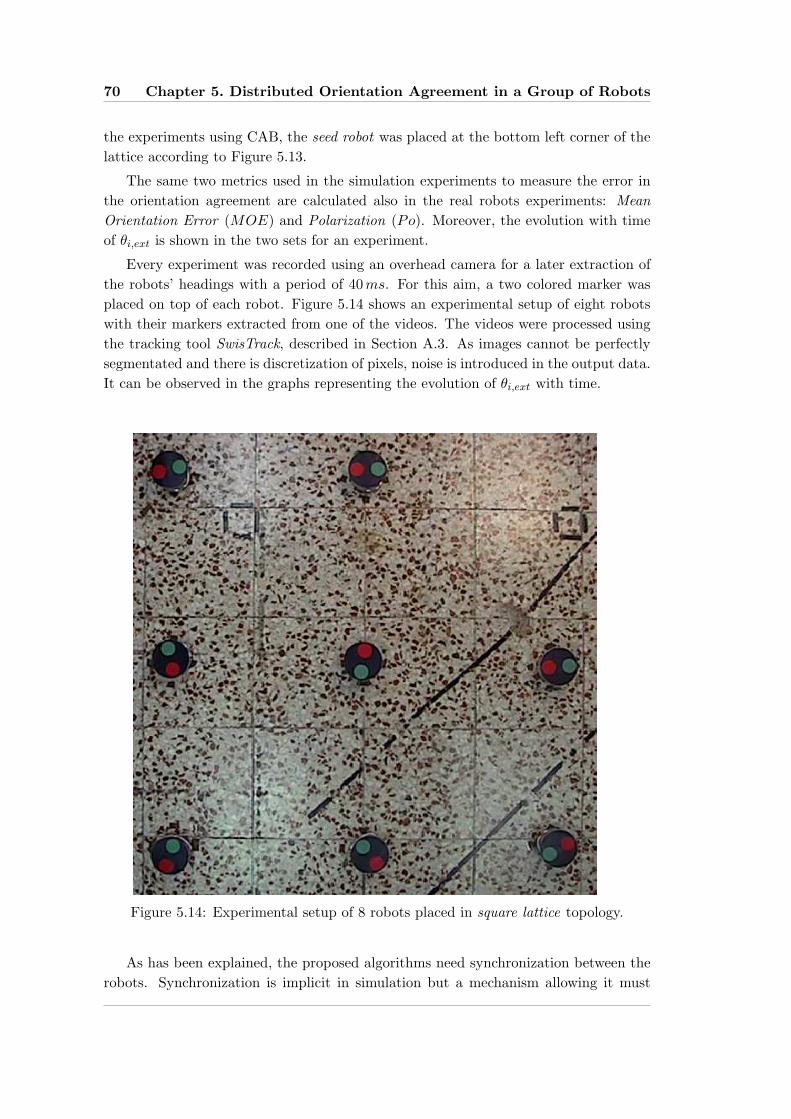
70 Chapter 5. Distributed Orientation Agreement in a Group of Robots
the experiments using CAB, the seed robot was placed at the bottom left corner of thelattice according to Figure 5.13.
The same two metrics used in the simulation experiments to measure the error inthe orientation agreement are calculated also in the real robots experiments: MeanOrientation Error (MOE) and Polarization (Po). Moreover, the evolution with timeof θi,ext is shown in the two sets for an experiment.
Every experiment was recorded using an overhead camera for a later extraction ofthe robots’ headings with a period of 40ms. For this aim, a two colored marker wasplaced on top of each robot. Figure 5.14 shows an experimental setup of eight robotswith their markers extracted from one of the videos. The videos were processed usingthe tracking tool SwisTrack, described in Section A.3. As images cannot be perfectlysegmentated and there is discretization of pixels, noise is introduced in the output data.It can be observed in the graphs representing the evolution of θi,ext with time.
Figure 5.14: Experimental setup of 8 robots placed in square lattice topology.
As has been explained, the proposed algorithms need synchronization between therobots. Synchronization is implicit in simulation but a mechanism allowing it must

5.5. Experiments with Real Robots 71
be performed in real robots. Several synchronization mechanisms exist, some reallydistributed and oriented towards wireless networks of the type that the set of robotsform. Finally, the Network Time Protocol (NTP) (Mills, 1992), the Internet standardfor time synchronization, was used because it is already implemented in the Linuxdistribution present in the robots. An external computer was used as NTP server, androbots synchronized with it at the beginning of the experiments. Its accuracy is in themillisecond scale, drifts are usually under 20ms.
In Section 5.5.1 and Section 5.5.2, the results for the two sets of experiments arepresented.
5.5.1 Set 1: CAA, Square Lattice Topology, α = 0.1, Alignment
In this set of experiments robots apply CAA as consensus algorithm, with α = 0.1. Thebehavior is alignment of its heading with the reference orientation estimate, this is thesame case as Set 3 of the simulation experiments but with eight robots. The placementtopology is square lattice. In Figure 5.15(a) the evolution of the headings of the robotsis plotted for a given experiment of this set. It can be seen that after time t = 5 s thedifference between them remains bounded. This can be better understood looking atFigure 5.15(b) and Figure 5.15(c) where Po and MOE are plotted with time for thesame experiment. Po(t) for t > 5 s remains under 0.3 rad and MOE(t) under 0.1 rad.
In Figure 5.15(d) the instantaneous maximum and the instantaneous mean of Po
and MOE of all the experiments of this set are shown. As it is shown in the figure, aftert = 5 s, the instantaneous maximum of Po remains under 0.5 rad, and the instantaneousmaximum of MOE remains under 0.15 rad, which shows that the 20 experimentsconverge. For t > 10 s, the mean value of Po for every experiment and for everytemporal step is 0.1448 rad. In the case of MOE this mean value is 0.0479 rad.
If this set is compared to its equivalent in simulation (Set 3, Figure 5.6), it canbe seen that the one with real robots converges much faster, since after 5 s Po andMOE are under 0.5 rad and 0.15 rad respectively, while in simulation it takes morethan 10 s to converge. This might be due to the difference in the number of robots,since here there are eight robots instead of 49. On the other hand, the maximum valuesof MOE and Po and the mean value of MOE and Po for every experiment and forevery temporal step is higher in the case of real robots. This can be due to a non perfectmodel of the relative positioning system in simulation, but also to noise introduced inthe tracking system. This idea is corroborated by the fact that robots in the video donot oscillate but in the plotting we see that robots do.
The variation of the heading with time due to the lack of perfect synchronicity, aswas shown in Set 9 of simulation experiments, is almost negligible in the case of theexperiment shown. The experiment of the set that has the largest variation of headingis approximately of 0.01 rad/s.

72 Chapter 5. Distributed Orientation Agreement in a Group of Robots
0 10 20 30 40 50 60−4
−3
−2
−1
0
1
2
3
4
time [s]
thet
a [r
ad]
(a) θi,ext(t) for a given experiment.
0 10 20 30 40 50 600
0.5
1
1.5
2
2.5
3
3.5
4
4.5
time [s]
pola
rizat
ion
[rad
]
(b) Po(t) for the same experiment.
0 10 20 30 40 50 600
0.2
0.4
0.6
0.8
1
1.2
1.4
1.6
time [s]
mea
n or
ient
atio
err
or [r
ad]
(c) MOE(t) for the same experiment.
0 10 20 30 40 50 600
1
2
3
4
5
6
time [s]
mea
n / m
ax [r
ad]
Mean MOEMax MOEMean polarizationMax polarization
(d) Instantaneous maximum and instantaneous
mean of Po and MOE of all the experiments.
Figure 5.15: Set 1: CAA, Square Lattice topology, α = 0.1, Alignment, real robots.
5.5.2 Set 2: CAB, Square Lattice Topology, α = 0.1, Alignment
In this set robots perform the alignment behavior, placed in square lattice topology,using the CAB algorithm with α = 0.1. The set is the same as Set 1 in simulation butusing CAB algorithm, and the same case as Set 8 in simulation but using eight realrobots instead of 49 simulated robots. In Figure 5.16(a) the evolution of θi,ext for eachrobot, for a given experiment is shown. Po and MOE are plotted with time for thesame experiment in Figure 5.16(b) and Figure 5.16(c).
The instantaneous maximum and the instantaneous mean of Po and MOE areplotted in Figure 5.16(d). From it we can see that after only 3 s these values are small,showing the fast convergence of all the 20 experiments of the set. The mean of Po
for every experiment and for every temporal step after t = 10 s is 0.1466 rad, whilethe maximum is 0.4580 rad. For MOE these values are 0.0490 rad for the mean and0.0972 rad for the maximum. These mean values are very similar to Set 1 with realrobots, which is normal since CAA and CAB behave very similar after they converge.
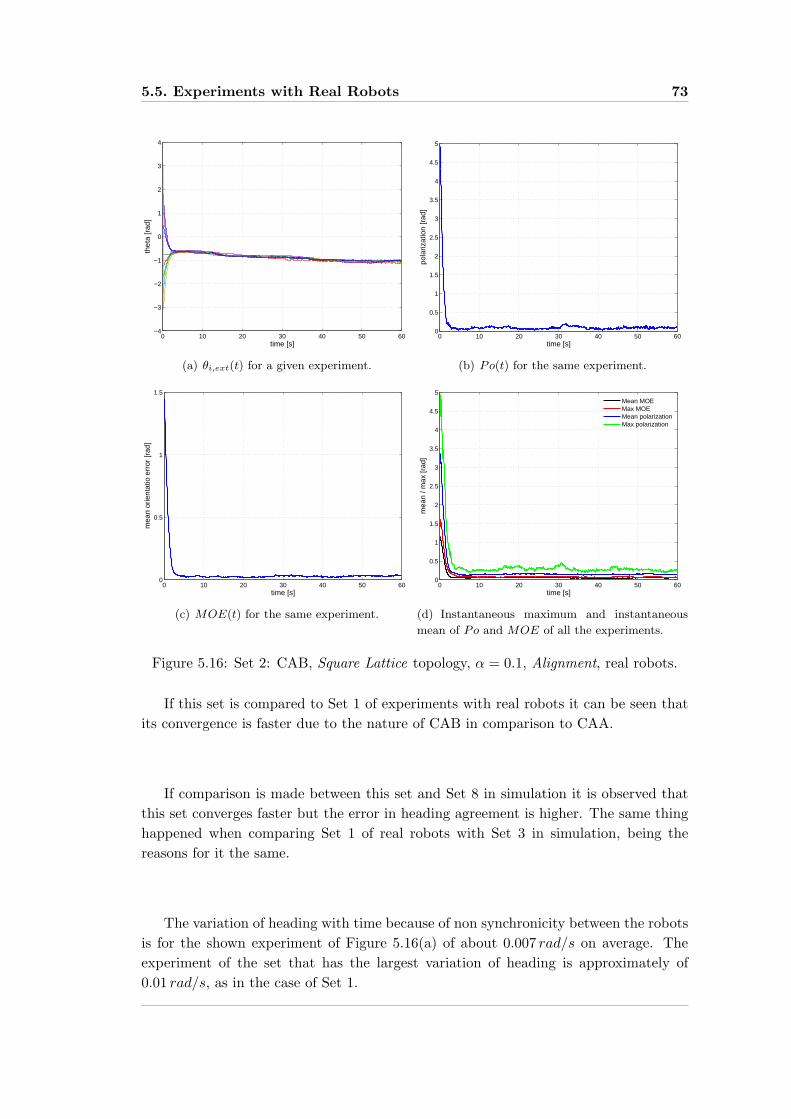
5.5. Experiments with Real Robots 73
0 10 20 30 40 50 60−4
−3
−2
−1
0
1
2
3
4
time [s]
thet
a [r
ad]
(a) θi,ext(t) for a given experiment.
0 10 20 30 40 50 600
0.5
1
1.5
2
2.5
3
3.5
4
4.5
5
time [s]
pola
rizat
ion
[rad
]
(b) Po(t) for the same experiment.
0 10 20 30 40 50 600
0.5
1
1.5
time [s]
mea
n or
ient
atio
err
or [r
ad]
(c) MOE(t) for the same experiment.
0 10 20 30 40 50 600
0.5
1
1.5
2
2.5
3
3.5
4
4.5
5
time [s]
mea
n / m
ax [r
ad]
Mean MOEMax MOEMean polarizationMax polarization
(d) Instantaneous maximum and instantaneous
mean of Po and MOE of all the experiments.
Figure 5.16: Set 2: CAB, Square Lattice topology, α = 0.1, Alignment, real robots.
If this set is compared to Set 1 of experiments with real robots it can be seen thatits convergence is faster due to the nature of CAB in comparison to CAA.
If comparison is made between this set and Set 8 in simulation it is observed thatthis set converges faster but the error in heading agreement is higher. The same thinghappened when comparing Set 1 of real robots with Set 3 in simulation, being thereasons for it the same.
The variation of heading with time because of non synchronicity between the robotsis for the shown experiment of Figure 5.16(a) of about 0.007 rad/s on average. Theexperiment of the set that has the largest variation of heading is approximately of0.01 rad/s, as in the case of Set 1.
74 Chapter 5. Distributed Orientation Agreement in a Group of Robots
5.6 Conclusions
In this chapter, a method for the agreement of a set of robots on a common referenceorientation based on a distributed algorithm has been described. Robots make only useof a relative positioning system, capable of detecting the positions of nearby robots,and local communications. Two different consensus algorithms based on the exchangeof information were proposed, tested and analyzed.
In order to test the method, systematic experiments were carried out in simulationand with real robots, varying the consensus algorithm, the α parameter of the consensusalgorithm, and the communication topology. The CAA consensus algorithm did notconverge in every experiment when robots were placed in ring topology. The successdepended on the initial conditions. On the other hand, CAB converged in everyexperiment for all the sets of experiments run. Its convergence has not been provedmathematically, but experimental results allow to trust the use of the algorithm. Atotal of 310 experiments of 60 s were performed: 270 of them in simulation and theremaining 40 using real robots.
Scalability with increasing number of robots, allowed by local communications andsensing, was tested successfully in simulation with up to 49 robots. All experimentswith real robots succeeded proving that the proposed method works with real robots.Experiments with a large group of real robots were not carried out, but the mentionedscalability in simulation and the nature (distributed, local communications and sensing)of the algorithms seems to indicate that it would work properly.
It has been seen that the use of large values of α makes convergence faster but theerror in the orientation agreement is bigger. This is not surprising since it implies afaster filter. Consequently, small values of α imply slow convergence but smaller error.
The method assumes synchronicity of the robots’ clocks. Experiments in simulationpurposely introduced delays among the robots’ clock, and experiments with real robotsinvolve imperfect synchronicity. This revealed that the algorithms worked properly,converging the reference orientation of all the robots, but that these values do notalways keep stable varying slowly with time. The maximum variation measured was0.01 rad/s.
One of the advantages of these methods is that if robots already posses a systemfor estimating the relative position of nearby robots, specific hardware is not required.In principle, the algorithm could work on any robot capable of detecting the positionof other robots and communicating with them.
The presence of a common orientation reference among all the robots of a groupcan be quite useful for some applications. It can be used, as will be seen in Chapter 6,as basis for flocking or other collective movement algorithms. The variation of thereference orientation with time because robots’ clocks might not be synchronized can becompatible with the use of the reference orientation in collective movement algorithms,if that variation is in the order of magnitude of the values measured in the experiments.
5.7. Future Work 75
5.7 Future Work
There are some works that in the future can complete and improve the developmentdescribed in this chapter. It is important to study rigorously the convergence of theCAB algorithm and, if necessary, modify it to ensure its convergence.
The algorithm could be modified to make it adaptive, being able to change the α
parameter, having a higher value in the beginning for a fast convergence, and a smallerone later on for more accuracy.
It would also be important to study what would happen if two different groups ofrobots would gather at a certain moment, since the confidences ci of all of them wouldbe already set to 1. One possible solution would be that one of the groups have a higherconfidence value than the other imposing its reference orientation to the other.
The method could also be complemented to add an origin point (0,0), which wouldimply having a complete coordinate system. Robots would need to keep track of allthe odometry values (not only θ), and also to exchange messages with this informationand the relative distances among them. Probably Kalman filters or a similar algorithmwould help in its implementation.

76 Chapter 5. Distributed Orientation Agreement in a Group of Robots
Chapter 6
Framework for Collective
Movement of Mobile Robots
Based on Distributed Decisions
If the people lead, the leaders will follow.
Unknown source
6.1 Introduction and Problem Statement
One of the main objectives of the Thesis is the design, development and implementationof a general framework for the collective movement of mobile robots. As stated inChapter 1, this framework must be scalable with the number of robots, which impliesthe use of local communications and sensing, as well as decentralized controllers (Sahin,2005). In addition, the functions that the framework should allow the group of robotsto carry out are: agreement in the group velocity; obstacle avoidance at group level;capacity of splitting in sub-groups and rejoining of sub-groups into a bigger group; andmodification and control of the external shape of the group. The framework shouldbe expandable, allowing to perform new functions, and it should be adaptive to newrequirements.
In this chapter, a framework for the collective movement of robots that fulfillsmost of the desired characteristics mentioned above, is explained, described, tested andanalyzed. The chapter is organized as follows. Firstly the restrictions and requirementsthat the robots must fulfill in order for the framework to work are defined in Section 6.2.The framework itself is described in Section 6.3, which after an introduction defines andexplains its basic controllers. Afterwards, it continues describing the several moduleswhich allow for the implementation of the different desired functions, and explains howthe framework works as a whole and how modules interact. Experiments in simulationshowing the different capabilities of the framework are presented in Section 6.4, whileexperiments performed with real robots are described in Section 6.5. The framework iscompared to previous related works from other researchers in Section 6.6. In Section 6.7,

78 Chapter 6. Framework for Collective Movement of Mobile Robots
the capabilities and properties of the framework are discussed. Lastly, the future linesof work, including possible applications of the framework are depicted in Section 6.8.
6.2 Robot Requirements for the Framework
In this section we state the capabilities that robots must fulfill so that the frameworkworks correctly. They are explained before the framework for an easier understanding.These basic requirements are grouped in the following sections according to their type:mobility, sensing and communications.
6.2.1 Robots’ Mobility
Robots must be able to perform translation movements in a two dimensional plane. Thelocomotion system of the robots used to test the framework is based on a differentialdrive system consisting of two motors and two wheels. Translation movements in atwo dimensional plane and rotations are allowed, with the kinematic restrictions of anunicycle vehicle. A wider description of the Khepera III robots used in the experimentscan be found in Section A.1. Two low level controllers specific for differential wheelvehicles are proposed in Section 6.3.2.2 and Section 6.3.2.3. Robots with a differentkinematic configuration can be used in the framework if new low level controllers aredesigned.
6.2.2 Robots’ Sensing
Regarding the sensing capabilities, robots must be able to detect the presence of nearbyobstacles by the use of distance sensors. The ultrasound and infra-red sensors of theKhepera III robots are used by different modules of the framework. If a different robotis used these modules must be reconfigured to cope with the differences of the sensorsof the new robot.
In addition, robots must be able to estimate the relative position of neighboringrobots. In the case of the experiments carried out to test the performance of theframework, this estimation is done by a relative positioning system, described in moredetail in Section A.1.1, based on the strength of the infrared signals interchanged byneighboring robots. The system is not only able to estimate the robots’ position butalso to communicate small messages between them. By the use of these messages,robots exchange a unique id, allowing not only to determine their relative positions butalso their ids, which is necessary for the proposed algorithms of the framework. Theestimation of the orientation of the nearby robots it is not needed by the framework.
6.2.3 Inter-Robot Communications
Robots need to communicate periodically with neighboring robots. In the case ofthe Khepera III robots used in the experiments, this is done using IEEE 802.11wireless standard and UDP messages. Any other systems which allow robot to robot
6.3. The Framework 79
communications, when robots are under a certain distance range, would be valid. Thisrange is determined by the desired inter-robot distance that the framework imposes.
6.3 The Framework
The designed and tested framework presented in this chapter allows the controlof the collective movement of a set of robots. As a result of robots running theframework controllers, the group of robots moves as a unique entity, being able toavoid obstacles, maintain a desired inter-robot distance, and decide collectively thedirection of movement and speed. The controller is distributed in each robot, and bothcommunications and sensing are local, which allows the scalability with an increasingnumber of robots. Robots are not placed in a perfect pre-defined formation whilemoving but try to maintain a desired inter-robot distance, forming a non perfecttriangular lattice.
The framework is based on four key parts:
• A common orientation reference system used by all the robots, which isimplemented using the distributed orientation agreement algorithms describedin Chapter 5. It could also be implemented using other mechanisms such asa compass or other localization mechanisms that allow the robots to share anreference orientation for all the robots.
• A basic distributed controller that makes the robots move as a group in adetermined direction while maintaining a desired inter-robot distance. Thiscontroller requires that robots share a common orientation reference.
• A distributed decision and general consensus protocol based on local commu-nications that allows to spread information and decisions from robots thathave preference, allowing to agree on different control parameters of the BasicController.
• A set of Modules which make use of the decision protocol, to decide and agreeon the values of certain parameters of the Basic Controller, allowing obstacleavoidance, speed control, or changing inter-robot distance.
The most important part of the framework is the coordination and communicationmechanism, implemented in the different modules, which allow future extensions withnew capabilities, and the implementation of more complicated tasks. The BasicController is not the most important part and could be replaced by a better one ifnecessary.
The resulting behavior of the group while moving collectively is similar to thebehavior of single robots moving according to the rules of simple reactive controllerssuch as those explained in Braitenberg (1984) and Arkin (1998), and in the bottomlayers of Brooks (1986). However, it can be used by higher level controllers to performmore complicated tasks, like odor source localization, mapping, exploration.

80 Chapter 6. Framework for Collective Movement of Mobile Robots
6.3.1 Common Orientation Agreement
As will be seen in Section 6.3.2, the Basic Controller needs that robots agree on thedesired direction of movement in order to work properly. One way to do that is toshare a reference orientation and agree on a direction angle referred to it. Robots sharea reference orientation when they use a global orientation system such as a magneticcompass, or use distributed methods for orientation agreement as those summarized inSection 5.1.
The method used and integrated in the framework is described and analyzed inChapter 5. In this method robots make use of a relative positioning system to detectnearby robots’ positions and local communications, which are also needed by the BasicController. This, together with the property of scalability with an increasing numberof robots, makes the method suitable for the framework.
6.3.2 Controllers
In this section the controllers in charge of collective movement are described andexplained. The Basic Controller, explained in Section 6.3.2.1, takes as input theposition of nearby robots and several variables shared among them, obtaining a desireddirection of movement expressed as a vector. This vector is taken as input by one ofthe two low level controllers described in Section 6.3.2.2 and Section 6.3.2.3. Theytransform the desired direction vector into wheels’ speed.
6.3.2.1 Basic Controller
This controller is in charge of the basic collective movement of the robots. Thecontroller’s output is a vector that indicates the desired direction of movement, whichdepends on several parameters, some shared variables and the positions of neighboringrobots. Some of these parameters are explained in the following lines for an easiercomprehension of the controller:
• Desired inter-robot distance (dd). As its name indicates, it is the desired distancethat robots must maintain between them.
• Desired group direction (θg) is the direction that the group of robots must take,referred to the common orientation reference.
• Kforward is a parameter that tunes the group speed. Larger values indicate fastergroup movement.
• Kaggregation is a parameter that weights the influence of robots trying to maintainthe desired inter-robot distance. The larger the value the faster they will react tothe error in the inter-robot distance.
The four of them are modified by different modules in order to control the inter-robotdistances and the group velocity.

6.3. The Framework 81
The controller output for a robot ri is a virtual velocity composed of two vectors:~vi,aggregation that is in charge of maintaining the desired inter-robot distance; and ~vi,group
that imposes the group direction movement.
~vi,total = ~vi,group + ~vi,aggregation (6.1)
~vi,group is the virtual velocity that moves robot ri in the desired group direction θg.It is a vector with the orientation θg, translated to the reference system of the robotand with a magnitude weighted by the Kforward parameter. Its magnitude and angleare defined by the following equations:
|~vi,group| = Kforward (6.2)
arg(vi,group) = θreference,i − θg (6.3)
where θreference,i is the estimate of the orientation reference.~vi,aggregation of robot ri is the weighted sum of the virtual velocities (~vi,j) for each
one of the robots rj being neighbors of type 1 or neighbors of type 2. Neighboring typeswill be explained afterwards.
~vi,aggregation =∑
∀j|rj∈type1
~vi,j +∑
∀j|rj∈type2
~vi,j (6.4)
The magnitude and angle of ~vi,j are defined as follows:
|~vi,j | = Kaggregation|di,j − dd| (6.5)
arg(vi,j) =
{θi,j , if di,j > dd
θi,j + π, if di,j ≤ dd
(6.6)
where di,j is the distance from robot ri to neighbor robot rj , and θi,j , as is defined inthe two previous chapters. So virtual velocity ~vi,j is an attractive vector towards robotrj if robots are further than the desired distance and repulsive if they are too close.
A visual explanation of ~vi,aggregation and vectors ~vi,j is depicted in Figure 6.1, where~vi,aggregation is calculated for ri = r0. Robots r1, r2 and r3 (in red) belong to type 1,robot r5 (in blue) to type 2, and robot r4 does not belong to any of the two types.
Robots rj belong to type 1 when their distance to robot ri is under a certain valueδ, they belong to the δ-neighborhood as defined in Section 4.2. The chosen value forδ is δ = 1.25dd, since in a perfect triangular lattice of inter-robot distance dd, nearestrobots that are not part of the same triangle are
√3dd away. Thus, by applying the sum
of ~vi,j , this is ~vi,aggregation, a triangular lattice formed by the robots’ positions mightarise. If robots being further than δ = 1.25dd were considered the group of robotswould tend to cluster, which is not the aim.
On the other hand, if robots further than δ = 1.25dd are not considered, andinitial positions among robots were further than δ, or a robot in the border of thegroup separates more than δ, the algorithm would not work. In order to overcome thisproblem, a solution that takes into account neighboring robots of type 2 was designed.

82 Chapter 6. Framework for Collective Movement of Mobile Robots
Figure 6.1: Schematic showing the ~vi,aggregation and ~vi,j for a set of six robots
The general idea behind the decision of neighboring robots of type 2 is similarto identifying locally robots that a priori do not belong to the same group from aconnection point of view, as the one described in Section 4.3.5.
The algorithm is simple. It takes initially as prospective robots of type 2 thoserobots rj that fulfill the following equation:
δ < di,j ≤ rrm ∗ dd (6.7)
where rrm is the relative maximum range which in the performed experiments is set torrm = 4. This means that prospective neighboring robots are situated inside a ring ofthe given inner and outer radius around ri.
The second condition for belonging to type 2 is that the angular distance of robotrj to every robot rk belonging to the δ-neighborhood of ri is larger than a thresholdangle thang. This condition is expressed as follows:
|θk,j | > thang, ∀k|rk ∈ Ni,δ (6.8)
where Ni,δ is the δ-neighborhood of ri.Figure 6.2 depicts the different parameters involved in determining of the type of
neighboring robots for a better comprehension. Neighboring robots of robot r0 of type1 are painted in red (r1, r2 and r3), and belong to zone 1, while those of type 2 arepainted in blue (r4, r5 and r6), and belong to zone 2.
Another point of view is that a robot ri would only have neighbors of type 2 ifit belongs to the border, and those neighboring robots are placed in the a directionseparated from the group to which ri belongs.
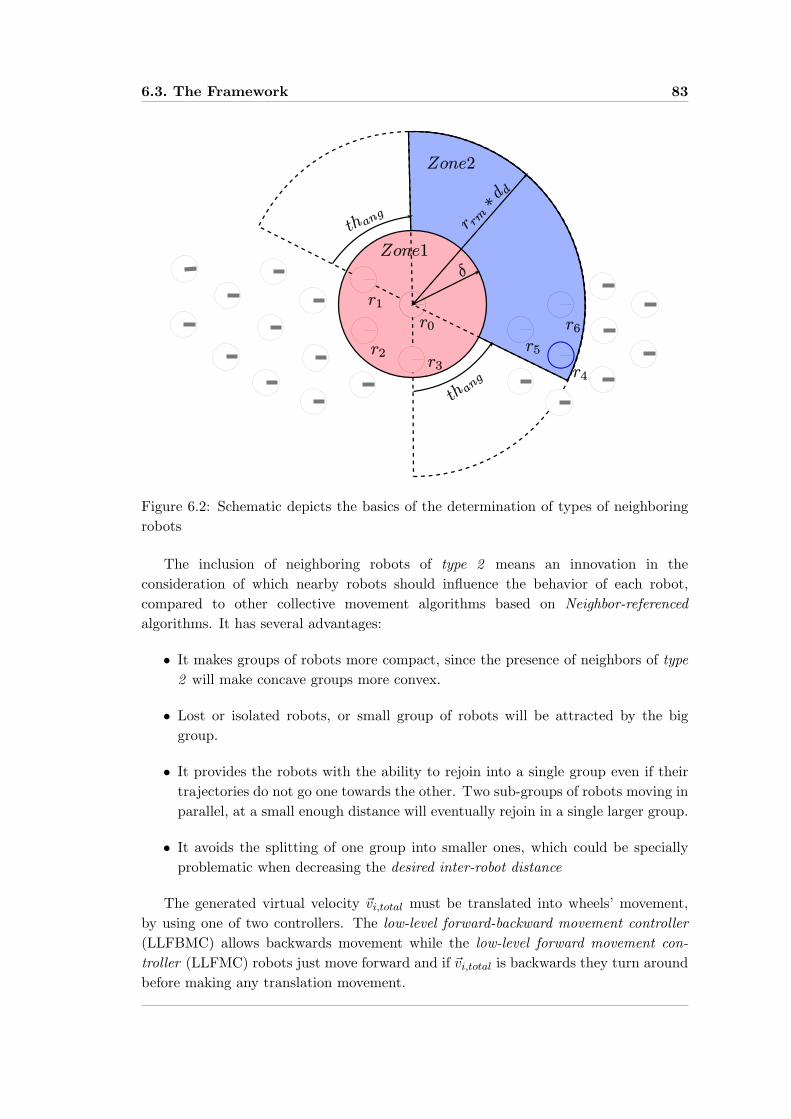
6.3. The Framework 83
Figure 6.2: Schematic depicts the basics of the determination of types of neighboringrobots
The inclusion of neighboring robots of type 2 means an innovation in theconsideration of which nearby robots should influence the behavior of each robot,compared to other collective movement algorithms based on Neighbor-referencedalgorithms. It has several advantages:
• It makes groups of robots more compact, since the presence of neighbors of type2 will make concave groups more convex.
• Lost or isolated robots, or small group of robots will be attracted by the biggroup.
• It provides the robots with the ability to rejoin into a single group even if theirtrajectories do not go one towards the other. Two sub-groups of robots moving inparallel, at a small enough distance will eventually rejoin in a single larger group.
• It avoids the splitting of one group into smaller ones, which could be speciallyproblematic when decreasing the desired inter-robot distance
The generated virtual velocity ~vi,total must be translated into wheels’ movement,by using one of two controllers. The low-level forward-backward movement controller(LLFBMC) allows backwards movement while the low-level forward movement con-troller (LLFMC) robots just move forward and if ~vi,total is backwards they turn aroundbefore making any translation movement.
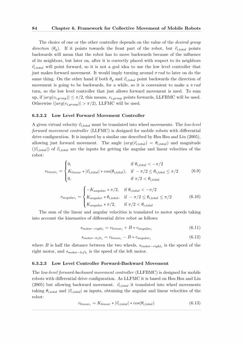
84 Chapter 6. Framework for Collective Movement of Mobile Robots
The choice of one or the other controller depends on the value of the desired groupdirection (θg). If it points towards the front part of the robot, but ~vi,total pointsbackwards will mean that the robot has to move backwards because of the influenceof its neighbors, but later on, after it is correctly placed with respect to its neighbors~vi,total will point forward, so it is not a god idea to use the low level controller thatjust makes forward movement. It would imply turning around π rad to later on do thesame thing. On the other hand if both θg and ~vi,total point backwards the direction ofmovement is going to be backwards, for a while, so it is convenient to make a π rad
turn, so the low level controller that just allows forward movement is used. To sumup, if |arg(vi,group)| ≤ π/2, this means, vi,group points forwards, LLFBMC will be used.Otherwise (|arg(vi,group)| > π/2), LLFMC will be used.
6.3.2.2 Low Level Forward Movement Controller
A given virtual velocity ~vi,total must be translated into wheel movements. The low-levelforward movement controller (LLFMC) is designed for mobile robots with differentialdrive configuration. It is inspired by a similar one described by Hsu Hsu and Liu (2005),allowing just forward movement. The angle (arg(~vi,total) = θi,total) and magnitude(|~vi,total|) of ~vi,total are the inputs for getting the angular and linear velocities of therobot:
vlineari =
0, if θi,total < −π/2
Klinear ∗ |~vi,total| ∗ cos(θi,total), if − π/2 ≤ θi,total ≤ π/2
0, if π/2 < θi,total
(6.9)
vangulari =
−Kangular ∗ π/2, if θi,total < −π/2
Kangular ∗ θi,total, if − π/2 ≤ θi,total ≤ π/2
Kangular ∗ π/2, if π/2 < θi,total
(6.10)
The sum of the linear and angular velocities is translated to motor speeds takinginto account the kinematics of differential drive robot as follows:
smotor−righti = vlineari+ B ∗ vangulari
(6.11)
smotor−lefti = vlineari −B ∗ vangulari (6.12)
where B is half the distance between the two wheels, smotor−righti is the speed of theright motor, and smotor−lefti is the speed of the left motor.
6.3.2.3 Low Level Controller Forward-Backward Movement
The low-level forward-backward movement controller (LLFBMC) is designed for mobilerobots with differential drive configuration. As LLFMC it is based on Hsu Hsu and Liu(2005) but allowing backward movement. ~vi,total it translated into wheel movementstaking θi,total and |~vi,total| as inputs, obtaining the angular and linear velocities of therobot:
vlineari = Klinear ∗ |~vi,total| ∗ cos(θi,total) (6.13)

6.3. The Framework 85
vangulari =
Kangular ∗ θi,total + π/2, if θi,total < −π/2
Kangular ∗ θi,total, if − π/2 ≤ θi,total ≤ π/2
Kangular ∗ θi,total − π/2, if π/2 < θi,total
(6.14)
The sum of the linear and angular velocities is translated to motor speeds using thesame equations as in LLFMC: Equation 6.11 and Equation 6.12.
6.3.3 Communication Systems
As previously said, two different communication systems coexist in the Khepera IIIrobots used to test the framework, the radio wireless system based on the IEEE 802.11standard, and the infra-red based system underlying the relative positioning system.The range of the wireless systems depends on the environment but it is around dozensof meters, while infra-red system’s range is 3.3m.
In order to allow scalability with an increasing number of robots, communicationsmust be kept local. We can imagine a situation in which 50 robots are placed forminga triangular lattice 2m side, given the range of the wireless system any robot wouldprobably be able to communicate with any other robot in the group, thus makingcommunications not very local. So in the implementation of the algorithm robots justtake into account wireless messages received from robots under a certain limited range.This range depends on dd, and is never larger than the limit of the relative positioningsystem, since distance information among robots is obtained from it.
Both communication systems form two parallel networks, whose links are limitedby the distance between robots. Messages are always sent from one robot to one of itscommunication neighbors. No routing protocol has been implemented. In Figure 6.3a schematic showing one of this networks is presented. The communication links ofrobot r0 are painted with a straight line, while communications links of other robot areindicated by dotted lines. The range area of the limited communications is painted ingreen.
Even if no routing protocols are used, information and consensus on several variablesspread over the network, by way of each robot receiving a message, processing it andsending messages in its turn to its neighbors. This is described in the following sections.
These two limited networks are used in the same way for the consensus on theorientation reference.
6.3.4 Variable Consensus
The Basic Controller takes four parameters (dd, θg, Kforward and Kaggregation) whichcontrol the inter-robot distance and the group velocity. For a correct performance ofthe algorithms robots must agree on the values of these parameters. If these valuesare set to a constant the controller will work but the direction of movement will beconstant, which makes the controller useless since it will not be able to avoid obstacles.The group of robots must be able to change these values according to the environmentor the objectives to carry out, at the same time as individuals agree on them.
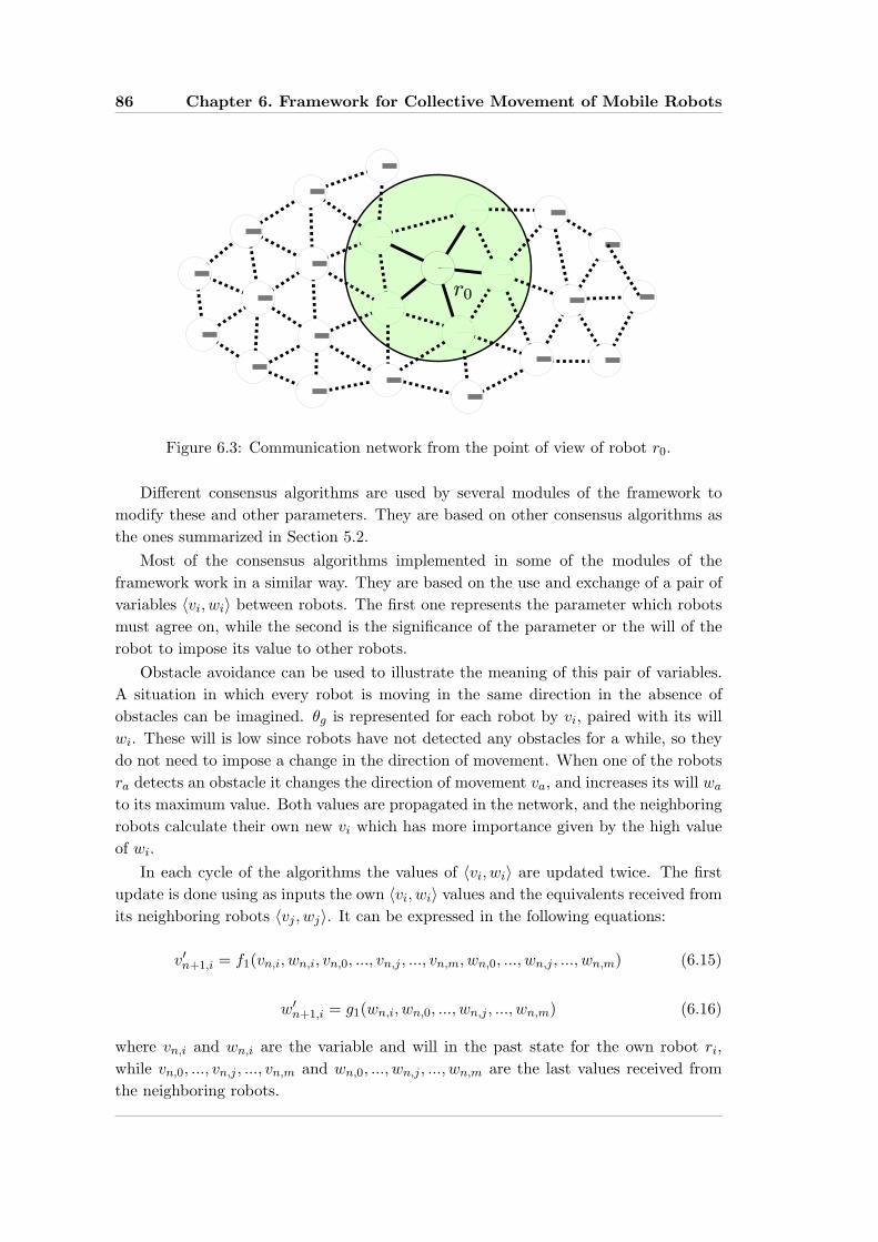
86 Chapter 6. Framework for Collective Movement of Mobile Robots
Figure 6.3: Communication network from the point of view of robot r0.
Different consensus algorithms are used by several modules of the framework tomodify these and other parameters. They are based on other consensus algorithms asthe ones summarized in Section 5.2.
Most of the consensus algorithms implemented in some of the modules of theframework work in a similar way. They are based on the use and exchange of a pair ofvariables 〈vi, wi〉 between robots. The first one represents the parameter which robotsmust agree on, while the second is the significance of the parameter or the will of therobot to impose its value to other robots.
Obstacle avoidance can be used to illustrate the meaning of this pair of variables.A situation in which every robot is moving in the same direction in the absence ofobstacles can be imagined. θg is represented for each robot by vi, paired with its willwi. These will is low since robots have not detected any obstacles for a while, so theydo not need to impose a change in the direction of movement. When one of the robotsra detects an obstacle it changes the direction of movement va, and increases its will wa
to its maximum value. Both values are propagated in the network, and the neighboringrobots calculate their own new vi which has more importance given by the high valueof wi.
In each cycle of the algorithms the values of 〈vi, wi〉 are updated twice. The firstupdate is done using as inputs the own 〈vi, wi〉 values and the equivalents received fromits neighboring robots 〈vj , wj〉. It can be expressed in the following equations:
v′n+1,i = f1(vn,i, wn,i, vn,0, ..., vn,j , ..., vn,m, wn,0, ..., wn,j , ..., wn,m) (6.15)
w′n+1,i = g1(wn,i, wn,0, ..., wn,j , ..., wn,m) (6.16)
where vn,i and wn,i are the variable and will in the past state for the own robot ri,while vn,0, ..., vn,j , ..., vn,m and wn,0, ..., wn,j , ..., wn,m are the last values received fromthe neighboring robots.

6.3. The Framework 87
In most of the consensus algorithms implemented, f1 is a weighted sum as thatexpressed in the next equation:
v′n+1,i = wn,i ∗ vn,i +∑
∀j|rj∈Ni,δ
wn,j ∗ vn,j (6.17)
In many modules, g1 is implemented as the maximum of the own will and the willsof the neighbors:
w′n+1,i = max(wn,i, wn,0, ..., wn,j , ..., wn,m) (6.18)
The second update has as inputs external events (e.g. the detection of an obstacle),and 〈v′n+1,i, w
′n+1,i〉 resulting from the first update. It also depends on the evolution
with time. It is expressed in the next equations:
vn+1,i = f2(v′n+1,i, t, events) (6.19)
wn+1,i = g2(w′n+1,i, t, events) (6.20)
After the two consequent updates of 〈vi, wi〉, vn+1,i and wn+1,i are sent to theneighboring robots.
The details on the implementation of f1, g1, f2 and g2 are given in each one of thefollowing modules that make use of consensus algorithms.
6.3.5 Modules Overview
The different modules explained in the following sections have the aim of improvingthe performance of the Basic Controller by adding new capabilities to the collectivemovement.
Most of the modules modify the different parameters of the Basic Controllercontroller or other variables that control the behavior of the group. Most of them makeuse of a distributed consensus algorithm similar to that explained in Section 6.3.4, butother make use of other mechanisms in order to modify the desired variables.
The Obstacle Avoidance Module (Section 6.3.7) controls the direction of movementof the group in order to avoid obstacle by using a consensus algorithm, while theSpeed Control Module (Section 6.3.8) controls the speed with a similar mechanism.The desired inter-robot distance is modified by the Inter-Robot Distance ControlModule (Section 6.3.9) also using a consensus algorithm. The Stop Control Module(Section 6.3.10) is in charge of deciding collectively if the group of robots must stopby using a consensus algorithm. The Splitting Control Module (Section 6.3.11) uses adifferent mechanism to split a group in two sub-groups.
The Individual Obstacle Avoidance Module (Section 6.3.6) is slightly different in itscoordination with the Basic Controller since it does not modify any of the parametersor variables, but takes control of the robot to avoid very close obstacles.
88 Chapter 6. Framework for Collective Movement of Mobile Robots
6.3.6 Individual Obstacle Avoidance Module
It is a very simple controller based on a Braitenberg (1984) architecture that takes asinputs just the values of the infra-red sensors of the robots, allowing the avoidance ofvery near obstacles.
The module is activated if the read value is over a threshold, i.e., when one ofthe infra-red sensors detects an object nearby. During its execution it supersedes theBasic Controller, which has no effect on the robot movement, but the communicationprotocols and updates of different variable by other modules continue working.
The equations that control the wheels’ speeds for a robot ri are the following:
smotor−righti = Kb1 +9∑
k=1
Kb2,k ∗ (sensorki + Kb3,k) (6.21)
smotor−lefti = Kb1 +9∑
k=1
Kb4,k ∗ (sensorki + Kb5,k) (6.22)
where k indicates the number of sensor, sensorki is the read value from sensor k of theown robot (ri). Kb1, Kb2,k, Kb3,k, Kb4,k and Kb5,k are constants set experimentally.
The algorithm was chosen since it had been already tested with real robots andin simulations and it performed very well, so there was no need for implementing andtesting a new one. Its integration in the framework improved the performance of thecollective movement, making robots behave as expected.
6.3.7 Obstacle Avoidance Module
The aim of this module is to control the group direction of movement (θg) in order toavoid the collisions with obstacles. It is implemented as a consensus algorithm basedon the generalities given in Section 6.3.4, using θg as the agreement variable (vi = θg).As in the general case, this consensus agreement makes use of the pair 〈vi, wi〉 updatedin two steps.
Since vi represents an angle, in the first update of vi according to f1, some specialconsideration must be taken into account because angles can not be added directly.Instead vi angles are converted to unit vectors with the direction of the angles. Wedenote ~vi as the unit vector of angle vi. Equation 6.15 can be implemented in a similarway to that shown in Equation 6.17:
~v′n+1,i = wn,i ∗ ~vn,i +∑
∀j|rj∈Ni,δ
wn,j ∗ ~vn,j (6.23)
The new intermediate estimation of v′n+1,i is calculated obtaining the angle of ~v′n+1,i:
v′n+1,i = arg(~v′n+1,i) (6.24)
The will is updated using Equation 6.18, calculating the maximum among the ownwill and the neighbors’ wills.
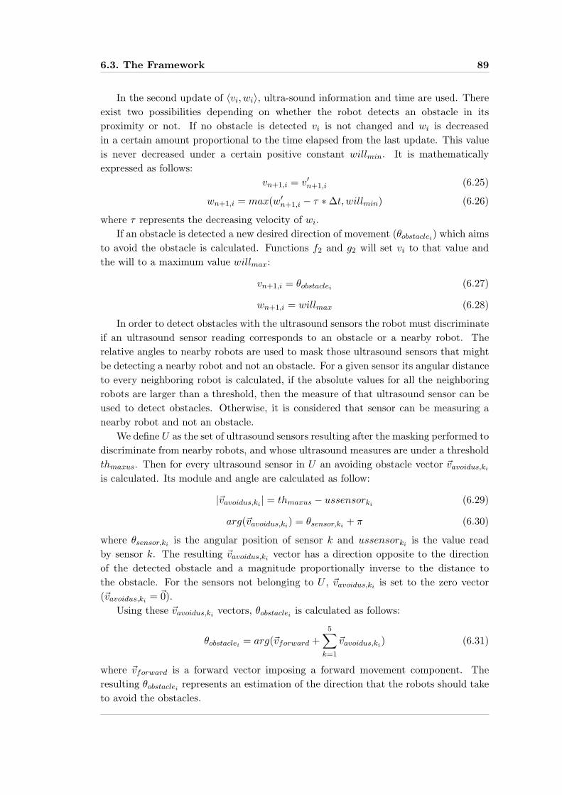
6.3. The Framework 89
In the second update of 〈vi, wi〉, ultra-sound information and time are used. Thereexist two possibilities depending on whether the robot detects an obstacle in itsproximity or not. If no obstacle is detected vi is not changed and wi is decreasedin a certain amount proportional to the time elapsed from the last update. This valueis never decreased under a certain positive constant willmin. It is mathematicallyexpressed as follows:
vn+1,i = v′n+1,i (6.25)
wn+1,i = max(w′n+1,i − τ ∗∆t, willmin) (6.26)
where τ represents the decreasing velocity of wi.If an obstacle is detected a new desired direction of movement (θobstaclei
) which aimsto avoid the obstacle is calculated. Functions f2 and g2 will set vi to that value andthe will to a maximum value willmax:
vn+1,i = θobstaclei (6.27)
wn+1,i = willmax (6.28)
In order to detect obstacles with the ultrasound sensors the robot must discriminateif an ultrasound sensor reading corresponds to an obstacle or a nearby robot. Therelative angles to nearby robots are used to mask those ultrasound sensors that mightbe detecting a nearby robot and not an obstacle. For a given sensor its angular distanceto every neighboring robot is calculated, if the absolute values for all the neighboringrobots are larger than a threshold, then the measure of that ultrasound sensor can beused to detect obstacles. Otherwise, it is considered that sensor can be measuring anearby robot and not an obstacle.
We define U as the set of ultrasound sensors resulting after the masking performed todiscriminate from nearby robots, and whose ultrasound measures are under a thresholdthmaxus. Then for every ultrasound sensor in U an avoiding obstacle vector ~vavoidus,ki
is calculated. Its module and angle are calculated as follow:
|~vavoidus,ki | = thmaxus − ussensorki (6.29)
arg(~vavoidus,ki) = θsensor,ki + π (6.30)
where θsensor,ki is the angular position of sensor k and ussensorki is the value readby sensor k. The resulting ~vavoidus,ki vector has a direction opposite to the directionof the detected obstacle and a magnitude proportionally inverse to the distance tothe obstacle. For the sensors not belonging to U , ~vavoidus,ki is set to the zero vector(~vavoidus,ki = ~0).
Using these ~vavoidus,ki vectors, θobstaclei is calculated as follows:
θobstaclei = arg(~vforward +5∑
k=1
~vavoidus,ki) (6.31)
where ~vforward is a forward vector imposing a forward movement component. Theresulting θobstaclei represents an estimation of the direction that the robots should taketo avoid the obstacles.
90 Chapter 6. Framework for Collective Movement of Mobile Robots
When a robot detects an obstacle it modifies its pair 〈vi, wi〉 setting vi to θobstaclei
and wi to a maximum value. It will propagate these values to its neighbors, whichwill copy wi since it is the maximum, and recalculate vi with a high influence of theneighbor that detected the obstacle for the same reason. In addition, these neighboringrobots will propagate their new influenced 〈vi, wi〉 that will have the same effect onother neighbors. This propagation of the θg can be better understood by looking atFigure 6.4. Every robot in the absence of obstacle detection will decrease its wi downto the minimum limit (willmin) in the lapse of seconds. In this manner they will beready to react to new obstacles. In absence of obstacle detection robots will continueexchanging the 〈vi, wi〉 for a better consensus on vi.
Figure 6.4: Schematics showing the propagation of θg with time, allowing obstacleavoidance.
The module was tested successfully as will be explained in sections 6.4 and 6.5.

6.3. The Framework 91
The group of robots change its direction of movement avoiding obstacles and wallswhen one or more robots detect them. The rest of the time they continue with straightmovement.
6.3.8 Speed Control Module
This module is in charge of controlling the group velocity by modifying in every robotthe value of Kforward parameter used by the Basic Controller. The objective is thatevery robot have the same value of Kforward, and that robots that posses relevantinformation about a change in the speed will influence the others. In order to dothat a consensus algorithm based on the generalities given in Section 6.3.4 has beenimplemented. The shared variable vi is set to Kforward.
The consensus algorithm is implemented in two steps as in the general case. Thefirst step uses the same Equation 6.17, and Equation 6.18 as in the general case. vi isupdated as a weighted sum of 〈vi, wi〉 and 〈vj , wj〉 of the neighbors. wi is set to themaximum of itself and the wj of the neighboring robots.
Robots start with a minimum value for will willmin and also a minimum valueregarding the speed vi = Kforwardmin . The aim is to accelerate if there are not obstaclesand to decrease immediately the speed to Kforward = Kforwardmin if an obstacle ispresent. The second update of 〈vi, wi〉 was implemented to ensure this behavior.
As in the Obstacle Avoidance Module there are two pair of equations to update〈vi, wi〉 depending if the robot ri has detected an obstacle or not. If no obstacle isdetected and wi = willmin, which means that for a while none of the robots has detectedan obstacle, then vi is increased a value proportional to the time elapsed from the lastupdate. If no obstacles have been detected but wi > willmin then vi is not changedin this step. wi in absence of obstacle detection is decreased an amount proportionalto the time elapsed down to wi = willmin. All of this is summarized in the followingequations:
vn+1,i =
{v′n+1,i, if wi > willmin
min(v′n+1,i + τ2 ∗∆t,Kforwardmax), if wi = willmin
(6.32)
wn+1,i = max(w′n+1,i − τ1 ∗∆t, willmin) (6.33)
where τ1 represents the increasing velocity of vi, this is, the group acceleration;Kforwardmax is the maximum Kforward allowed; and τ2 is the decreasing velocity ofwi. In the absence of obstacles the robot will accelerate but for security the will isminimum in order to react fast to the presence of an obstacle.
If an obstacle is detected then the robot must decrease immediately its velocity andinfluence its neighbors. Functions f2 and g2 will set vi to the minimum value and wi
to the maximum:
vn+1,i = Kforwardmin (6.34)
wn+1,i = willmax (6.35)
92 Chapter 6. Framework for Collective Movement of Mobile Robots
The detection of obstacles is carried out by the Obstacle Avoidance Module andit does not represent a problem since the Speed Control Module is always used inconjunction with it. If it is used separately then the obstacle detection should be doneautonomously.
Other events or conditions could have been considered for controlling the groupspeed. For instance the error in the inter-robot distance could have been used,increasing the speed if the error is low and decreasing otherwise.
The module was tested both in simulation and with real robots, as will be detailedin the related sections, observing the desired behavior of acceleration in the absence ofobstacle up to a maximum speed, and fast deceleration if obstacles are detected.
6.3.9 Inter-Robot Distance Control Module
The aim of this module is to modify the desired inter-robot distance (dd) in order totest that the Basic Controller is capable of successfully dealing with that.
As in the previous modules, a consensus algorithm was designed and implementedto modify the parameter under study, with vi = dd. The difference of this modulewith the others is that the conditions to change vi in the second update, do not onlydepend on external sensor readings but are function of the previous value and time,i.e., vn+1,i = f2(v′n+1,i, t). In addition this modifications is performed only by one ofthe robots, which acts as a leader imposing its desired inter-robot distance over therest of the group. The implication of this is twofold:
• The propagation vi originated only in one robot can be tested in large groups,which could allow the presence of leaders for some desired tasks. Somehow thischaracteristic is already tested when only one robot detects an obstacle in theObstacle Avoidance Module.
• It shows a mechanism that allows the teleoperation of the group of robots byjust sending commands to one of the robots. In the explained case there exist nocommands, and decisions are taken in one of the robots.
The first update of vi of the consensus algorithm is performed using the sameequations 6.17 and 6.18 as in the general case and other modules. vi is updated as aweighted sum and wi is set to the maximum of itself and wj of the neighboring robots.
Robots that are not the leader leave vi unchanged in the second update of thealgorithm and decrease wi an amount proportional to the elapsed time since the lastupdate. The leader robot updates 〈vi, wi〉 in the same manner in most of the cycles.This update is defined in equations 6.25 and 6.26, since they are the same as those usedin the Obstacle Avoidance Module in the absence of obstacles.
Periodically the leader robot modifies the desired inter-robot distance expressed invi according to an internal function h(t), and sets wi to its maximum value (willmax)in order to propagate vi through the group of robots.
vn+1,i = h(t) (6.36)

6.3. The Framework 93
wn+1,i = willmax (6.37)
This type of update takes place with a period T , and in the rest of the updates vi isnot modified and wi is decreased as explained before.
The leader robot does modify vi every step to allow to propagate the value byletting wi decrease. The consensus and modification of vi is implemented as fast wavesthat start in the leader and propagate through the group, copying the desired value ofvi given by the leader and agreeing on it.
The dd given by h(t) and imposed periodically by the leader robot is copied bythe group of robots that agree on the value. This is the reason why the describedmechanism can be used for teleoperation of the group of robots by modifying othervariables. The h(t) functions used were periodic functions of several types (sinusoidal,triangular, squared), with period 45 s and inter-robot distances between 0.5m and2.5m. Some of these results are described in the experimental sections.
The algorithm could be modified to change the desired inter-robot distanceaccording to external events or properties of the flock. For instance by checking theinter-robot distance error, or the presence of obstacles in the same place for a while, therobots could estimate if they are inside a corridor an decrease their inter-robot distancefor an easier pass through it.
6.3.10 Stop Control Module
This module is in charge of deciding collectively if the group of robots must stop. Thisdecision is made taking into account if there are many robots very close to obstacles, thisis, running the Individual Obstacle Avoidance Module. It uses a consensus algorithmvery similar to that explained before, in which vi indicates whether robots must moveby a positive value or must stop by a negative one. The range of vi is [−1, 1]. Whena robot thinks that the group must stop it sets vi = −1 and wi = willmax. If a robotwants the group to continue moving it sets vi = 1 and wi = willmax.
The first update of vi and wi of the consensus algorithm is carried out using thesame equations 6.17 and 6.18 as in the general case and other modules.
The second update takes as input a variable that indicates if the robot is usingthe Individual Obstacle Avoidance Module, this is if there are near obstacles aroundit. It uses the information about itself and about its neighboring robots. If more thanthN robots out of the neighboring robots and itself are using the Individual ObstacleAvoidance Module then the robot decides the group must stop by updating vi and wi
as follows:vn+1,i = −1 (6.38)
wn+1,i = willmax (6.39)
If a robot has been stopped for a certain time then the second update of theconsensus algorithm updates vi and wi to allow movement of itself and the rest:
vn+1,i = 1 (6.40)
wn+1,i = willmax (6.41)

94 Chapter 6. Framework for Collective Movement of Mobile Robots
If there is no need to change the state of the group, this is to stop the movement orrestart it, then the second update of the consensus algorithm is given by equations 6.25and 6.26, which decrease wi and leave vi unchanged.
Each cycle robots check vi, stopping if its value is negative and letting the BasicController move them if it is positive.
The module was tested only on simulation with successful results. Robots placedin a complicated and small area started to use the Individual Obstacle AvoidanceModule, coming the group to stop moving. After a certain time the group restarted itsmovement.
This consensus algorithm demonstrates that discrete decisions can be done in adistributed way. Similar mechanisms could be used to make distributed decisions.
6.3.11 Splitting Control Module
This module allows the splitting of a group of robots into two subgroups. The aim ofthe module is just to demonstrate that the framework and the controllers are able tomake the group of robots split, but the decision on when to split and in which manneris given arbitrarily by one of the robots. No work has been done on deciding accordingto the perceived environment when and how to split, this is left for future works. Thismodule is not based at all on any consensus algorithm.
The splitting mechanism is done by making a part of the group of robots belong toone group and the other part to a different one. This is shown in the group variable. Ifone robot detects a nearby robot of a group different from its own group then it doesnot consider it as a neighboring robot. The Basic Controller, the orientation referenceconsensus and any other consensus mechanism do not consider that nearby robot. Inaddition the Obstacle Avoidance Module will consider that robot as an obstacle andwill try to avoid it. So, if in a group of robots some of them change their group variablethe group will split and the new two subgroups will separate from each other.
In order to split the group, one of the robots establish a line that divides the group;robots at one side belong to one sub-group (group = 1), and robots at the other sideto the other (group = 2). This line is defined by its orientation (θline) relative to thecommon orientation reference, and the minimum distance (~dline,i), positive or negative,to the line from the robot, this is the perpendicular vector from a robot to the line. Aschematic showing it is depicted on Figure 6.5.
The robot that decides to split calculates the ~dline,j of its neighboring robots, usingthe relative bearing to them and ~dline,i and θline. Then it sends to them ~dline,j togetherwith the group numbers and θline. These neighboring robots do the same with itsneighbors and the information propagates and robots set their new group. After thatthe group split into two sub-groups that move away from each other thanks to thepresence of the Obstacle Avoidance Module.
This module was tested both in simulation and with real robots with successfulresults shown in the experimental sections.

6.3. The Framework 95
Figure 6.5: Splitting into two sub-groups overview.
6.3.12 Workings of the Framework
In Figure 6.6, a schematic that summarizes the relations between the controllers, thedifferent modules and the common orientation agreement algorithm is shown. Thearrows represent the flow of information from the modules to the controllers, indicatingthe variable or parameter that is modified in the controller.
Depending on the combination of modules which are activated, the group of robotswill behave in a different manner. If no module is running and the different parametersof the Basic Controller are the same in all the robots then the group of robots will movein a straight direction, speed and inter-robot distance both approximately constant.This is useful in order to test the capabilities of the controller. For safer operation itis useful to add the functionality of the Individual Obstacle Avoidance Module to avoidcollisions and damages in the robots.
In order to make the movement more intelligent, the Obstacle Avoidance Modulecan be added while maintaining the Individual Obstacle Avoidance Module. In this waythe group of robots will be able to avoid obstacles collectively by changing the groupdirection of movement. The group speed will be almost constant.
The last case can be improved by adding the Speed Control Module allowing thegroup of robots to accelerate in the absence of obstacles, and to slow down if obstaclesare detected to reduce the risk of collisions.
The inclusion of the the Stop Control Module module will complete the previousconfiguration allowing it to stop the robots when they are stuck in a local minimumhelping them to scape from that situation by restarting the movement.
The rest of the modules, the Inter-Robot Distance Control Module, and the SplittingControl Module are not developed enough for practical applications and should bepreviously enhanced with more autonomous capabilities. They demonstrate thecapability of the framework to implement those functions.

96 Chapter 6. Framework for Collective Movement of Mobile Robots
Figure 6.6: Schematic showing the relations between the controllers, the differentmodules and the common orientation agreement algorithm. Arrows indicate the flowof information
6.4 Experiments in Simulation
In order to test and show the capabilities of the proposed framework, several setsof experiments were carried out in simulation, using the Webots simulator (moreinformation in Section A.2) and a dynamic model of the Khepera III robot. Eachone of these sets is composed of a total of 30 experiments of 60 s, and makes use ofa different combination of framework’s modules in order to test how they work. Sixsets of experiments are performed using 40 robots, with the aim of demonstrating thescalability with an increasing number of robots. Another six use only eight robots inorder to compare them with experiments with real robots in which only eight robotsare present, using the same parameters as those with eight robots.
In all the experiments the consensus algorithm for agreement in the orientationreference used was CAB, with an α = 0.05. The parameters of the low level controllersare fixed in all the experiments. If a robot is perfectly placed with respect to itsneighboring robots, this is, Kaggregation = 0, then the Khepera III robot should moveforward with a speed of 0.178Kforward m/s. This value is going to be used as a referenceto compare the group speed. The rest of parameters of the Basic Controller and of themodules are different depending on the modules under test. The Individual ObstacleAvoidance Module is present in all the experiments since it is the basic mechanism of
6.4. Experiments in Simulation 97
security that avoids collisions.In the simulations performed robots read the relative positions of their neighbors,
they update their sensor readings and update their motor commands every 128ms.They also exchange wireless messages every 128ms, which are received by theirneighboring robots with a delay of 128ms. The bearing accuracy of the relativepositioning system is modelled with an additive Gaussian noise of standard deviationσ = 0.2 rad, while the distance has a standard deviation 15%.
Robots are initially placed forming a square lattice of 0.5m distance between robots,and with randomly uniformly distributed headings, in all the sets of experiments exceptone that tests how groups rejoin.
The performance of the experiments is measured using most of the metrics describedand proposed in Chapter 4. Some of them are presented as a function of time for asingle example, while others are given as an statistic. In addition, for some experimentsthe trajectories of the robots are shown.
6.4.1 Basic Collective Movement
The first step to check the capabilities of the framework is to test the Basic Controllerwithout the inclusion of any module besides the Individual Obstacle Avoidance Modulefor security reasons. Two different sets of experiments were done using exactly the sameparameters, but using 8 robots in one case and 40 in the other. Robots should movetogether in a constant direction trying to maintain the desired inter-robot distance(dd). Initially, the headings of the robots should be different for a later agreementon the desired direction. The relevant parameters of the Basic Controller used are:Kforward = 1, Kaggregation = 0.8 and dd = 0.7m. In Table 6.1, the main characteristicsof the sets under study are summarized.
In order to understand the dynamics of the algorithm different metrics are shownin Figure 6.7 with time for a single experiment with 40 robots. In Figure 6.7(b), thegroup speed (GS) is presented, showing that just after a few seconds it reaches analmost constant value 0.17 m/s. On the other hand the mean distance error (MDE)which indicates the error in the inter-robot desired distance with neighbors averagedfor every robot takes around 45 s to stabilize (Figure 6.7(d)), since robots are placed inan area smaller than it should be and it takes some time until they reach the desiredpositions. Using a larger Kaggregation would make MDE decrease faster, but probablyGS would not be maximum so fast. Differences in the headings are given by polarization(Po, Figure 6.7(c)) and mean orientation error (MOE, Figure 6.7(e)) decreasing quitefast. In order to give a glimpse on the movement of the robots, their trajectories areshown in Figure 6.7(a), showing quite straight paths.
The relevant statistics for this sets of experiments are presented in Table 6.2.They are calculated for each set of experiments for all the experiments for t > 5 s.Average means average for all the time steps after the desired initial time and for allthe experiments. The same applies referred to the standard deviation. Path lengthratio (PLR) is not related with time, so it is calculated using the starting positionof the robots for t = 0. Its average and standard deviation are calculated for the 30

98 Chapter 6. Framework for Collective Movement of Mobile Robots
−12 −10 −8 −6 −4 −2 0 2 40
0.5
1
1.5
2
2.5
3
3.5
4
x [m]
y [m
]
(a) Trajectories of the robots during the experiment. The initial positions of the robots are marked
with a small circle (right), while the final positions are marked with a square (left).
0 10 20 30 40 50 600
0.05
0.1
0.15
0.2
0.25
time [s]
spee
d [m
/s]
(b) GroupSpeed(t) for the same experiment.
0 10 20 30 40 50 600
0.5
1
1.5
2
2.5
3
3.5
4
time [s]
pola
rizat
ion
[rad
]
(c) Polarization(t) for the same experiment.
0 10 20 30 40 50 600.05
0.06
0.07
0.08
0.09
0.1
0.11
0.12
0.13
time [s]
mea
n di
stan
ce e
rror
[m]
(d) MeanDistanceError(t) for the same experi-
ment.
0 10 20 30 40 50 600
0.2
0.4
0.6
0.8
1
1.2
1.4
time [s]
mea
n or
ient
atio
n er
ror
[rad
]
(e) MeanOrientationError(t) for the same exper-
iment.
Figure 6.7: Relevant metrics and robots’ trajectories shown for a single experiment ofSet1-40-sim tested in simulation.
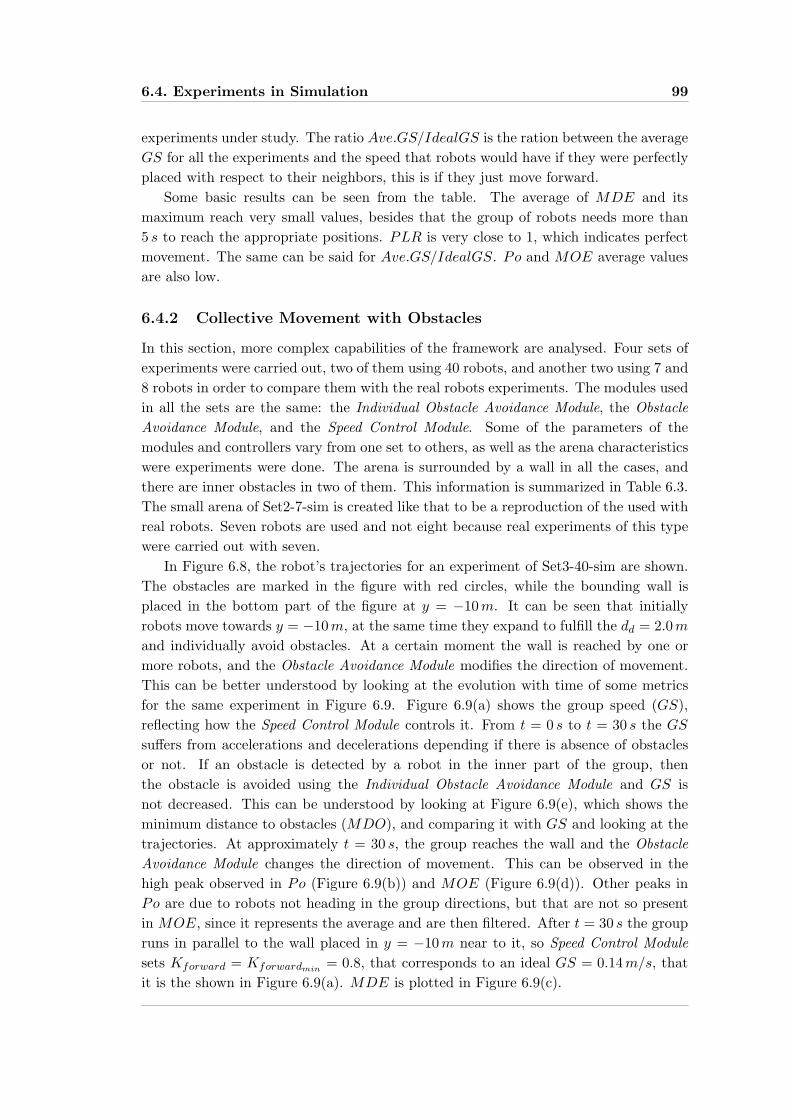
6.4. Experiments in Simulation 99
experiments under study. The ratio Ave.GS/IdealGS is the ration between the averageGS for all the experiments and the speed that robots would have if they were perfectlyplaced with respect to their neighbors, this is if they just move forward.
Some basic results can be seen from the table. The average of MDE and itsmaximum reach very small values, besides that the group of robots needs more than5 s to reach the appropriate positions. PLR is very close to 1, which indicates perfectmovement. The same can be said for Ave.GS/IdealGS. Po and MOE average valuesare also low.
6.4.2 Collective Movement with Obstacles
In this section, more complex capabilities of the framework are analysed. Four sets ofexperiments were carried out, two of them using 40 robots, and another two using 7 and8 robots in order to compare them with the real robots experiments. The modules usedin all the sets are the same: the Individual Obstacle Avoidance Module, the ObstacleAvoidance Module, and the Speed Control Module. Some of the parameters of themodules and controllers vary from one set to others, as well as the arena characteristicswere experiments were done. The arena is surrounded by a wall in all the cases, andthere are inner obstacles in two of them. This information is summarized in Table 6.3.The small arena of Set2-7-sim is created like that to be a reproduction of the used withreal robots. Seven robots are used and not eight because real experiments of this typewere carried out with seven.
In Figure 6.8, the robot’s trajectories for an experiment of Set3-40-sim are shown.The obstacles are marked in the figure with red circles, while the bounding wall isplaced in the bottom part of the figure at y = −10 m. It can be seen that initiallyrobots move towards y = −10 m, at the same time they expand to fulfill the dd = 2.0m
and individually avoid obstacles. At a certain moment the wall is reached by one ormore robots, and the Obstacle Avoidance Module modifies the direction of movement.This can be better understood by looking at the evolution with time of some metricsfor the same experiment in Figure 6.9. Figure 6.9(a) shows the group speed (GS),reflecting how the Speed Control Module controls it. From t = 0 s to t = 30 s the GS
suffers from accelerations and decelerations depending if there is absence of obstaclesor not. If an obstacle is detected by a robot in the inner part of the group, thenthe obstacle is avoided using the Individual Obstacle Avoidance Module and GS isnot decreased. This can be understood by looking at Figure 6.9(e), which shows theminimum distance to obstacles (MDO), and comparing it with GS and looking at thetrajectories. At approximately t = 30 s, the group reaches the wall and the ObstacleAvoidance Module changes the direction of movement. This can be observed in thehigh peak observed in Po (Figure 6.9(b)) and MOE (Figure 6.9(d)). Other peaks inPo are due to robots not heading in the group directions, but that are not so presentin MOE, since it represents the average and are then filtered. After t = 30 s the groupruns in parallel to the wall placed in y = −10m near to it, so Speed Control Modulesets Kforward = Kforwardmin = 0.8, that corresponds to an ideal GS = 0.14m/s, thatit is the shown in Figure 6.9(a). MDE is plotted in Figure 6.9(c).
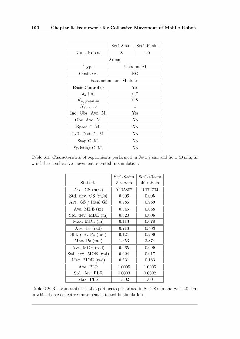
100 Chapter 6. Framework for Collective Movement of Mobile Robots
Set1-8-sim Set1-40-sim
Num. Robots 8 40
Arena
Type Unbounded
Obstacles NO
Parameters and Modules
Basic Controller Yesdd (m) 0.7
Kaggregation 0.8Kforward 1
Ind. Obs. Avo. M. Yes
Obs. Avo. M. No
Speed C. M. No
I.-R. Dist. C. M. No
Stop C. M. No
Splitting C. M. No
Table 6.1: Characteristics of experiments performed in Set1-8-sim and Set1-40-sim, inwhich basic collective movement is tested in simulation.
Set1-8-sim Set1-40-simStatistic 8 robots 40 robots
Ave. GS (m/s) 0.175807 0.172704Std. dev. GS (m/s) 0.006 0.005Ave. GS / Ideal GS 0.986 0.969
Ave. MDE (m) 0.045 0.058Std. dev. MDE (m) 0.020 0.006
Max. MDE (m) 0.113 0.078
Ave. Po (rad) 0.216 0.563Std. dev. Po (rad) 0.121 0.296
Max. Po (rad) 1.653 2.874
Ave. MOE (rad) 0.065 0.099Std. dev. MOE (rad) 0.024 0.017
Max. MOE (rad) 0.331 0.183
Ave. PLR 1.0005 1.0005Std. dev. PLR 0.0003 0.0002
Max. PLR 1.002 1.001
Table 6.2: Relevant statistics of experiments performed in Set1-8-sim and Set1-40-sim,in which basic collective movement is tested in simulation.
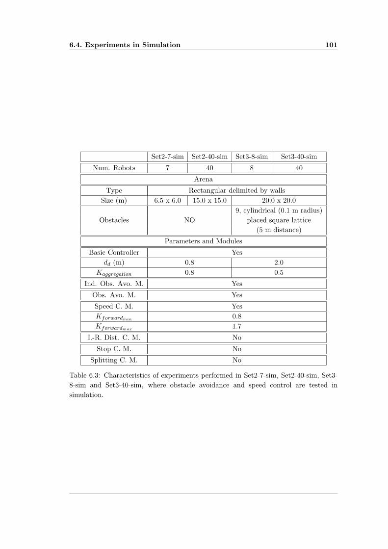
6.4. Experiments in Simulation 101
Set2-7-sim Set2-40-sim Set3-8-sim Set3-40-sim
Num. Robots 7 40 8 40
Arena
Type Rectangular delimited by wallsSize (m) 6.5 x 6.0 15.0 x 15.0 20.0 x 20.0
9, cylindrical (0.1 m radius)Obstacles NO placed square lattice
(5 m distance)
Parameters and Modules
Basic Controller Yesdd (m) 0.8 2.0
Kaggregation 0.8 0.5
Ind. Obs. Avo. M. Yes
Obs. Avo. M. Yes
Speed C. M. YesKforwardmin 0.8Kforwardmax 1.7
I.-R. Dist. C. M. No
Stop C. M. No
Splitting C. M. No
Table 6.3: Characteristics of experiments performed in Set2-7-sim, Set2-40-sim, Set3-8-sim and Set3-40-sim, where obstacle avoidance and speed control are tested insimulation.

102 Chapter 6. Framework for Collective Movement of Mobile Robots
−8 −6 −4 −2 0 2 4 6 8−10
−8
−6
−4
−2
0
2
4
x [m]
y [m
]
Figure 6.8: Trajectories of the robots during an experiment of Set3-40-sim whereobstacle avoidance and speed control are tested in simulation. The initial positionsof the robots are marked with a small circle, while the final positions are marked witha square. Visible obstacles are marked with red circles.

6.4. Experiments in Simulation 103
0 10 20 30 40 50 600
0.05
0.1
0.15
0.2
0.25
time [s]
spee
d [m
/s]
(a) GroupSpeed(t) for an experiment.
0 10 20 30 40 50 600
0.5
1
1.5
2
2.5
3
3.5
4
4.5
time [s]
pola
rizat
ion
[rad
]
(b) Polarization(t) for the same experiment.
0 10 20 30 40 50 600.25
0.3
0.35
0.4
0.45
0.5
0.55
0.6
0.65
time [s]
mea
n di
stan
ce e
rror
[m]
(c) MeanDistanceError(t) for the same experi-
ment.
0 10 20 30 40 50 600
0.5
1
1.5
time [s]
mea
n or
ient
atio
n er
ror
[rad
]
(d) MeanOrientationError(t) for the same exper-
iment.
0 10 20 30 40 50 60−0.1
0
0.1
0.2
0.3
0.4
0.5
0.6
time [s]
min
imum
dis
tanc
e to
obs
tacl
es [m
]
(e) MinimumDistancetoObstacles(t) for the same
experiment.
Figure 6.9: Relevant metrics shown for an experiment of Set3-40-sim where obstacleavoidance and speed control are tested in simulation.
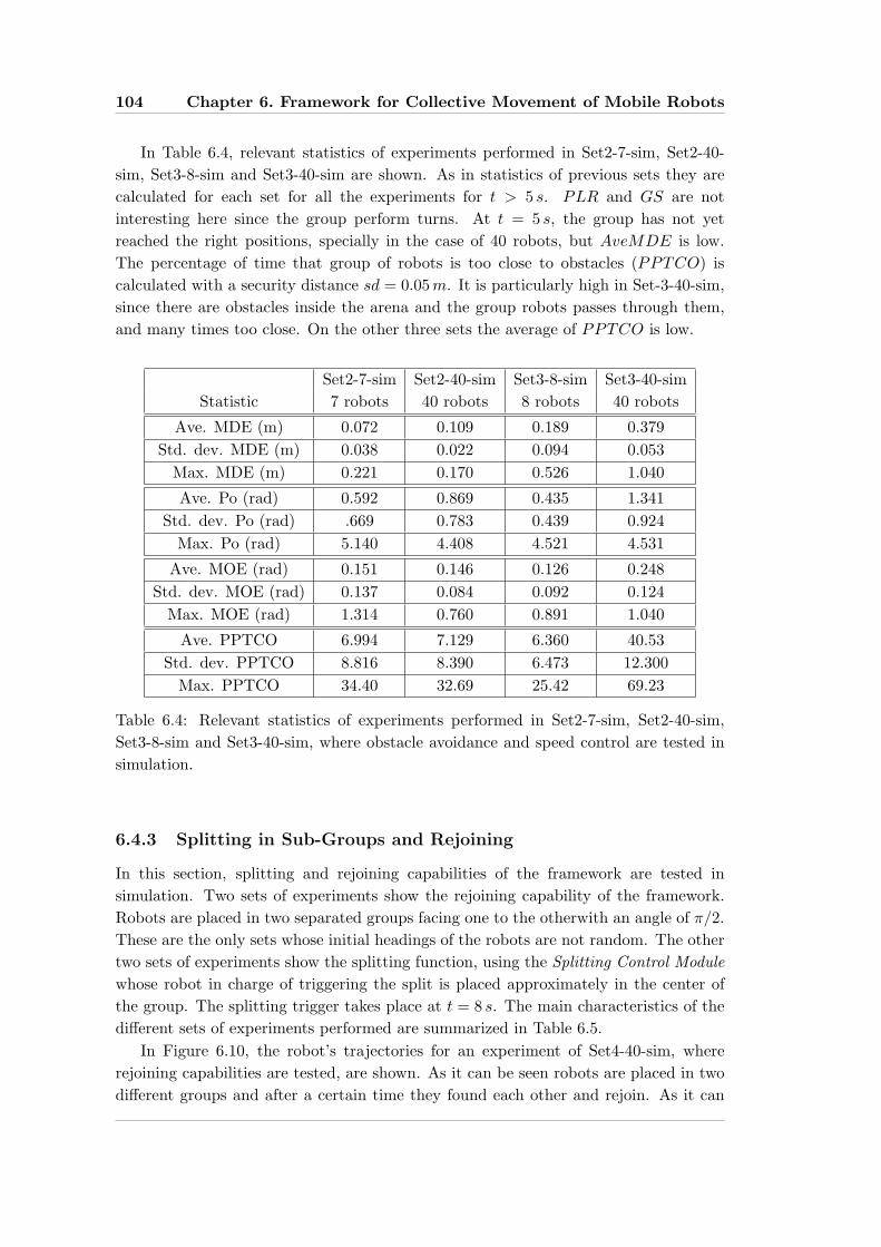
104 Chapter 6. Framework for Collective Movement of Mobile Robots
In Table 6.4, relevant statistics of experiments performed in Set2-7-sim, Set2-40-sim, Set3-8-sim and Set3-40-sim are shown. As in statistics of previous sets they arecalculated for each set for all the experiments for t > 5 s. PLR and GS are notinteresting here since the group perform turns. At t = 5 s, the group has not yetreached the right positions, specially in the case of 40 robots, but AveMDE is low.The percentage of time that group of robots is too close to obstacles (PPTCO) iscalculated with a security distance sd = 0.05m. It is particularly high in Set-3-40-sim,since there are obstacles inside the arena and the group robots passes through them,and many times too close. On the other three sets the average of PPTCO is low.
Set2-7-sim Set2-40-sim Set3-8-sim Set3-40-simStatistic 7 robots 40 robots 8 robots 40 robots
Ave. MDE (m) 0.072 0.109 0.189 0.379Std. dev. MDE (m) 0.038 0.022 0.094 0.053
Max. MDE (m) 0.221 0.170 0.526 1.040
Ave. Po (rad) 0.592 0.869 0.435 1.341Std. dev. Po (rad) .669 0.783 0.439 0.924
Max. Po (rad) 5.140 4.408 4.521 4.531
Ave. MOE (rad) 0.151 0.146 0.126 0.248Std. dev. MOE (rad) 0.137 0.084 0.092 0.124
Max. MOE (rad) 1.314 0.760 0.891 1.040
Ave. PPTCO 6.994 7.129 6.360 40.53Std. dev. PPTCO 8.816 8.390 6.473 12.300
Max. PPTCO 34.40 32.69 25.42 69.23
Table 6.4: Relevant statistics of experiments performed in Set2-7-sim, Set2-40-sim,Set3-8-sim and Set3-40-sim, where obstacle avoidance and speed control are tested insimulation.
6.4.3 Splitting in Sub-Groups and Rejoining
In this section, splitting and rejoining capabilities of the framework are tested insimulation. Two sets of experiments show the rejoining capability of the framework.Robots are placed in two separated groups facing one to the otherwith an angle of π/2.These are the only sets whose initial headings of the robots are not random. The othertwo sets of experiments show the splitting function, using the Splitting Control Modulewhose robot in charge of triggering the split is placed approximately in the center ofthe group. The splitting trigger takes place at t = 8 s. The main characteristics of thedifferent sets of experiments performed are summarized in Table 6.5.
In Figure 6.10, the robot’s trajectories for an experiment of Set4-40-sim, whererejoining capabilities are tested, are shown. As it can be seen robots are placed in twodifferent groups and after a certain time they found each other and rejoin. As it can
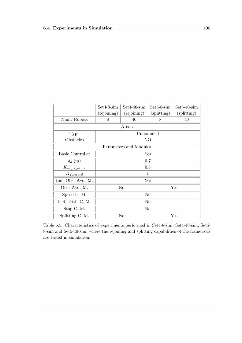
6.4. Experiments in Simulation 105
Set4-8-sim Set4-40-sim Set5-8-sim Set5-40-sim(rejoining) (rejoining) (splitting) (splitting)
Num. Robots 8 40 8 40
Arena
Type UnboundedObstacles NO
Parameters and Modules
Basic Controller Yes
dd (m) 0.7Kaggregation 0.8Kforward 1
Ind. Obs. Avo. M. Yes
Obs. Avo. M. No Yes
Speed C. M. No
I.-R. Dist. C. M. No
Stop C. M. No
Splitting C. M. No Yes
Table 6.5: Characteristics of experiments performed in Set4-8-sim, Set4-40-sim, Set5-8-sim and Set5-40-sim, where the rejoining and splitting capabilities of the frameworkare tested in simulation.
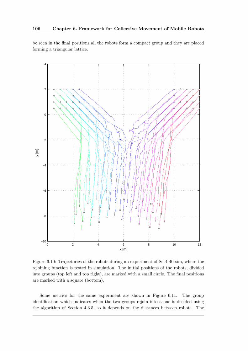
106 Chapter 6. Framework for Collective Movement of Mobile Robots
be seen in the final positions all the robots form a compact group and they are placedforming a triangular lattice.
0 2 4 6 8 10 12−10
−8
−6
−4
−2
0
2
4
x [m]
y [m
]
Figure 6.10: Trajectories of the robots during an experiment of Set4-40-sim, where therejoining function is tested in simulation. The initial positions of the robots, dividedinto groups (top left and top right), are marked with a small circle. The final positionsare marked with a square (bottom).
Some metrics for the same experiment are shown in Figure 6.11. The groupidentification which indicates when the two groups rejoin into a one is decided usingthe algorithm of Section 4.3.5, so it depends on the distances between robots. The
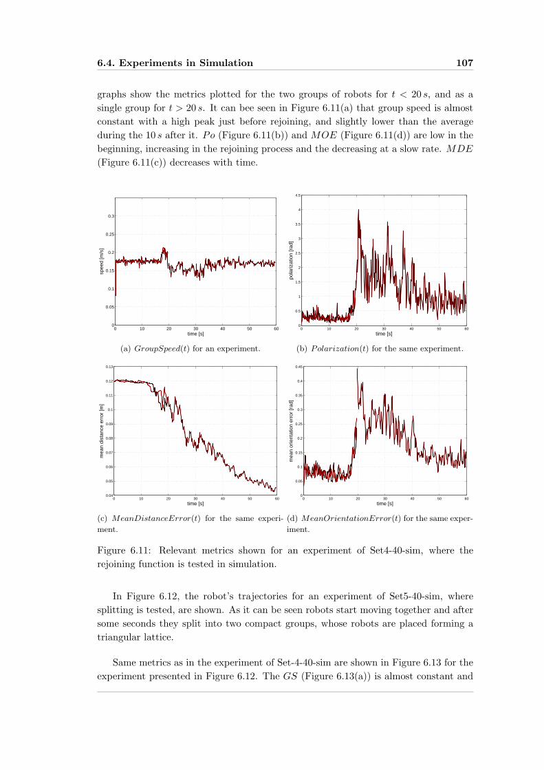
6.4. Experiments in Simulation 107
graphs show the metrics plotted for the two groups of robots for t < 20 s, and as asingle group for t > 20 s. It can bee seen in Figure 6.11(a) that group speed is almostconstant with a high peak just before rejoining, and slightly lower than the averageduring the 10 s after it. Po (Figure 6.11(b)) and MOE (Figure 6.11(d)) are low in thebeginning, increasing in the rejoining process and the decreasing at a slow rate. MDE
(Figure 6.11(c)) decreases with time.
0 10 20 30 40 50 600
0.05
0.1
0.15
0.2
0.25
0.3
time [s]
spee
d [m
/s]
(a) GroupSpeed(t) for an experiment.
0 10 20 30 40 50 600
0.5
1
1.5
2
2.5
3
3.5
4
4.5
time [s]
pola
rizat
ion
[rad
]
(b) Polarization(t) for the same experiment.
0 10 20 30 40 50 600.04
0.05
0.06
0.07
0.08
0.09
0.1
0.11
0.12
0.13
time [s]
mea
n di
stan
ce e
rror
[m]
(c) MeanDistanceError(t) for the same experi-
ment.
0 10 20 30 40 50 600
0.05
0.1
0.15
0.2
0.25
0.3
0.35
0.4
0.45
time [s]
mea
n or
ient
atio
n er
ror
[rad
]
(d) MeanOrientationError(t) for the same exper-
iment.
Figure 6.11: Relevant metrics shown for an experiment of Set4-40-sim, where therejoining function is tested in simulation.
In Figure 6.12, the robot’s trajectories for an experiment of Set5-40-sim, wheresplitting is tested, are shown. As it can be seen robots start moving together and aftersome seconds they split into two compact groups, whose robots are placed forming atriangular lattice.
Same metrics as in the experiment of Set-4-40-sim are shown in Figure 6.13 for theexperiment presented in Figure 6.12. The GS (Figure 6.13(a)) is almost constant and

108 Chapter 6. Framework for Collective Movement of Mobile Robots
−5 0 5 100
2
4
6
8
10
12
x [m]
y [m
]
Figure 6.12: Trajectories of the robots during an experiment of Set5-40-sim, where thesplitting function is tested in simulation. The initial positions of the robots are markedwith a small circle (bottom). The final positions, where robots are split into two groups(top left and top right) are marked with a square.
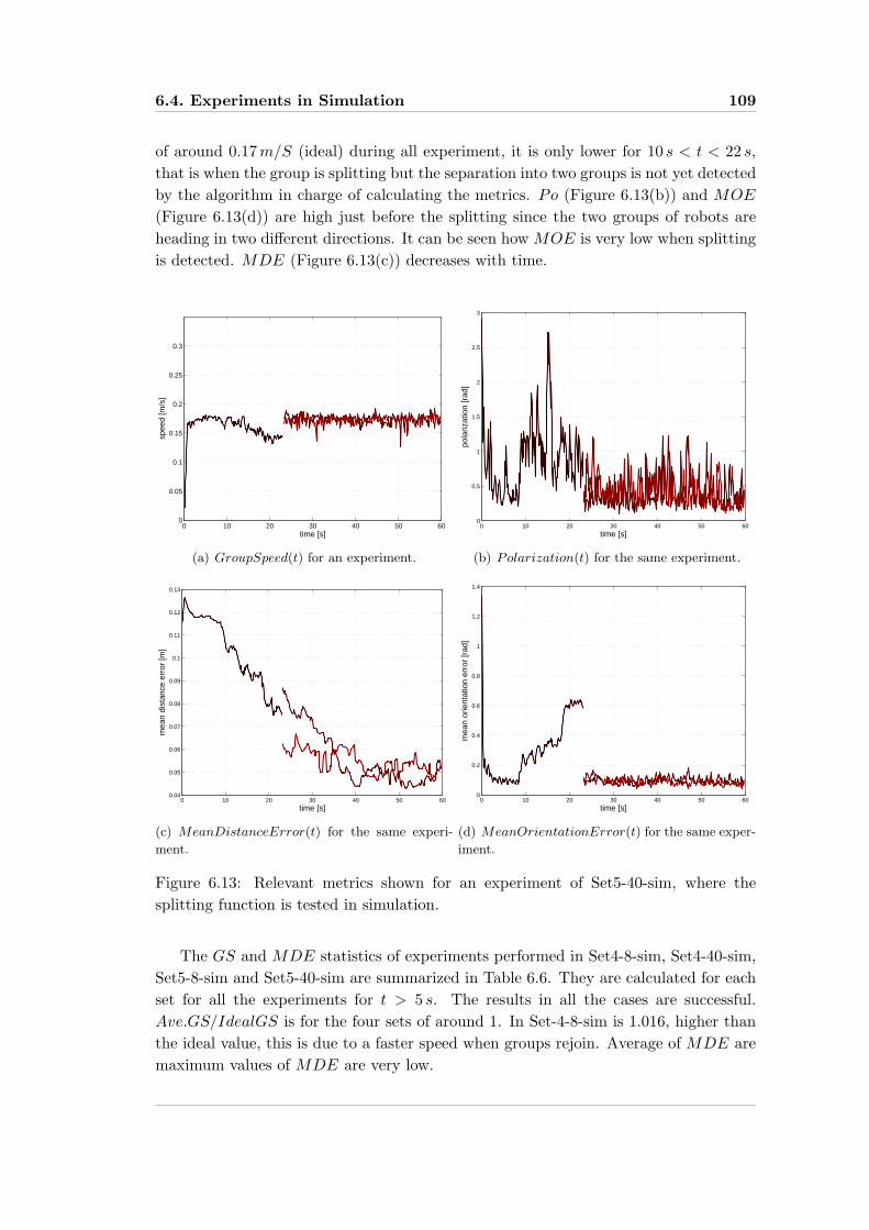
6.4. Experiments in Simulation 109
of around 0.17m/S (ideal) during all experiment, it is only lower for 10 s < t < 22 s,that is when the group is splitting but the separation into two groups is not yet detectedby the algorithm in charge of calculating the metrics. Po (Figure 6.13(b)) and MOE
(Figure 6.13(d)) are high just before the splitting since the two groups of robots areheading in two different directions. It can be seen how MOE is very low when splittingis detected. MDE (Figure 6.13(c)) decreases with time.
0 10 20 30 40 50 600
0.05
0.1
0.15
0.2
0.25
0.3
time [s]
spee
d [m
/s]
(a) GroupSpeed(t) for an experiment.
0 10 20 30 40 50 600
0.5
1
1.5
2
2.5
3
time [s]
pola
rizat
ion
[rad
]
(b) Polarization(t) for the same experiment.
0 10 20 30 40 50 600.04
0.05
0.06
0.07
0.08
0.09
0.1
0.11
0.12
0.13
time [s]
mea
n di
stan
ce e
rror
[m]
(c) MeanDistanceError(t) for the same experi-
ment.
0 10 20 30 40 50 600
0.2
0.4
0.6
0.8
1
1.2
1.4
time [s]
mea
n or
ient
atio
n er
ror
[rad
]
(d) MeanOrientationError(t) for the same exper-
iment.
Figure 6.13: Relevant metrics shown for an experiment of Set5-40-sim, where thesplitting function is tested in simulation.
The GS and MDE statistics of experiments performed in Set4-8-sim, Set4-40-sim,Set5-8-sim and Set5-40-sim are summarized in Table 6.6. They are calculated for eachset for all the experiments for t > 5 s. The results in all the cases are successful.Ave.GS/IdealGS is for the four sets of around 1. In Set-4-8-sim is 1.016, higher thanthe ideal value, this is due to a faster speed when groups rejoin. Average of MDE aremaximum values of MDE are very low.
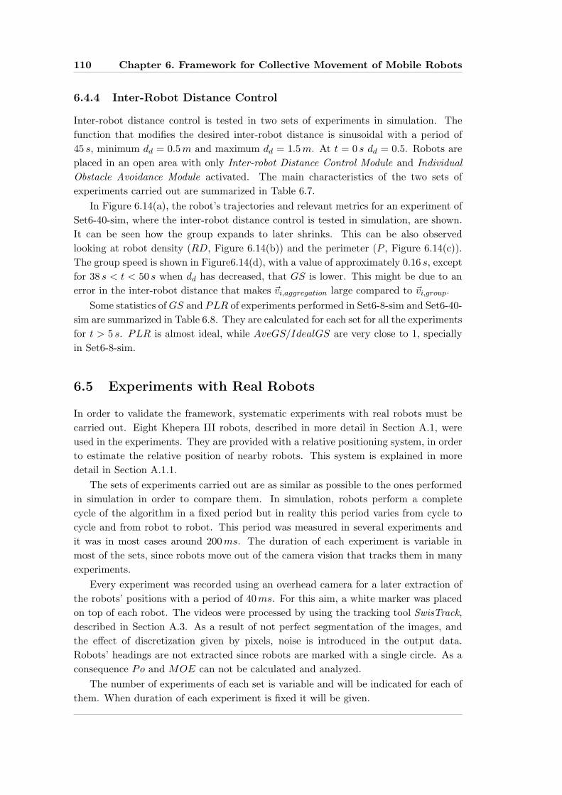
110 Chapter 6. Framework for Collective Movement of Mobile Robots
6.4.4 Inter-Robot Distance Control
Inter-robot distance control is tested in two sets of experiments in simulation. Thefunction that modifies the desired inter-robot distance is sinusoidal with a period of45 s, minimum dd = 0.5m and maximum dd = 1.5m. At t = 0 s dd = 0.5. Robots areplaced in an open area with only Inter-robot Distance Control Module and IndividualObstacle Avoidance Module activated. The main characteristics of the two sets ofexperiments carried out are summarized in Table 6.7.
In Figure 6.14(a), the robot’s trajectories and relevant metrics for an experiment ofSet6-40-sim, where the inter-robot distance control is tested in simulation, are shown.It can be seen how the group expands to later shrinks. This can be also observedlooking at robot density (RD, Figure 6.14(b)) and the perimeter (P , Figure 6.14(c)).The group speed is shown in Figure6.14(d), with a value of approximately 0.16 s, exceptfor 38 s < t < 50 s when dd has decreased, that GS is lower. This might be due to anerror in the inter-robot distance that makes ~vi,aggregation large compared to ~vi,group.
Some statistics of GS and PLR of experiments performed in Set6-8-sim and Set6-40-sim are summarized in Table 6.8. They are calculated for each set for all the experimentsfor t > 5 s. PLR is almost ideal, while AveGS/IdealGS are very close to 1, speciallyin Set6-8-sim.
6.5 Experiments with Real Robots
In order to validate the framework, systematic experiments with real robots must becarried out. Eight Khepera III robots, described in more detail in Section A.1, wereused in the experiments. They are provided with a relative positioning system, in orderto estimate the relative position of nearby robots. This system is explained in moredetail in Section A.1.1.
The sets of experiments carried out are as similar as possible to the ones performedin simulation in order to compare them. In simulation, robots perform a completecycle of the algorithm in a fixed period but in reality this period varies from cycle tocycle and from robot to robot. This period was measured in several experiments andit was in most cases around 200ms. The duration of each experiment is variable inmost of the sets, since robots move out of the camera vision that tracks them in manyexperiments.
Every experiment was recorded using an overhead camera for a later extraction ofthe robots’ positions with a period of 40ms. For this aim, a white marker was placedon top of each robot. The videos were processed by using the tracking tool SwisTrack,described in Section A.3. As a result of not perfect segmentation of the images, andthe effect of discretization given by pixels, noise is introduced in the output data.Robots’ headings are not extracted since robots are marked with a single circle. As aconsequence Po and MOE can not be calculated and analyzed.
The number of experiments of each set is variable and will be indicated for each ofthem. When duration of each experiment is fixed it will be given.
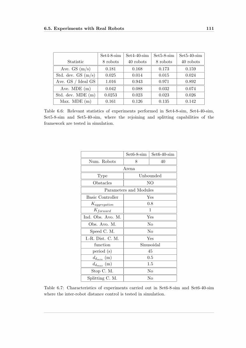
6.5. Experiments with Real Robots 111
Set4-8-sim Set4-40-sim Set5-8-sim Set5-40-simStatistic 8 robots 40 robots 8 robots 40 robots
Ave. GS (m/s) 0.181 0.168 0.173 0.159Std. dev. GS (m/s) 0.025 0.014 0.015 0.024Ave. GS / Ideal GS 1.016 0.943 0.971 0.892
Ave. MDE (m) 0.042 0.088 0.032 0.074Std. dev. MDE (m) 0.0253 0.023 0.023 0.026
Max. MDE (m) 0.161 0.126 0.135 0.142
Table 6.6: Relevant statistics of experiments performed in Set4-8-sim, Set4-40-sim,Set5-8-sim and Set5-40-sim, where the rejoining and splitting capabilities of theframework are tested in simulation.
Set6-8-sim Set6-40-sim
Num. Robots 8 40
Arena
Type Unbounded
Obstacles NO
Parameters and Modules
Basic Controller YesKaggregation 0.8Kforward 1
Ind. Obs. Avo. M. Yes
Obs. Avo. M. No
Speed C. M. No
I.-R. Dist. C. M. Yesfunction Sinusoidal
period (s) 45ddmin (m) 0.5ddmax (m) 1.5
Stop C. M. No
Splitting C. M. No
Table 6.7: Characteristics of experiments carried out in Set6-8-sim and Set6-40-simwhere the inter-robot distance control is tested in simulation.

112 Chapter 6. Framework for Collective Movement of Mobile Robots
−10 −8 −6 −4 −2 0 2 4−2
−1
0
1
2
3
4
5
x [m]
y [m
]
(a) Trajectories of the robots during the experiment.
0 10 20 30 40 50 601
1.5
2
2.5
3
3.5
4
4.5
5
5.5
6
time [s]
robo
t den
sity
[num
ber
of r
obot
s/m
2]
(b) RobotDensity(t) for the same experiment.
0 10 20 30 40 50 6010
12
14
16
18
20
22
time [s]
perim
eter
[m]
(c) Perimeter(t) for the same experiment.
0 10 20 30 40 50 600
0.05
0.1
0.15
0.2
0.25
time [s]
spee
d [m
/s]
(d) GroupSpeed(t) for the same experiment.
Figure 6.14: Relevant metrics and robots’ trajectories shown for an experiment ofSet6-40-sim. The inter-robot distance control is tested in simulation.

6.5. Experiments with Real Robots 113
6.5.1 Basic Collective Movement
As in the simulation case, the first thing to do is testing the Basic Controller togetherwith the Individual Obstacle Avoidance Module. Two sets of experiments, both usingeight robots and composed of 10 experiments each, were carried out. Set1-8-real hasthe same parameters as Set1-8-sim of simulation in order to be able to compare them.Set1b-8-real differs on dd and Kaggregation. The duration of each experiments is notfixed. Both sets are summarized in Table 6.9.
In Figure 6.15(a), the robot’s trajectories for an experiment of Set1-8-real are shown.It can be seen in last step positions how robots form a triangular lattice. GS is shownin Figure 6.15(b), being quite stable for t > 2 s. Part of the fluctuation observed canbe due to the pixelation introduced by the tracking system. Figure 6.15(c) plots theMDE that remains quite small for t > 10 s.
Similar information is shown in Figure 6.16 for an experiment of Set1b-8-real.Trajectories are found in Figure 6.16(a). GS is plotted in Figure 6.15(b), beingalso quite constant. MDE is presented in Figure 6.15(c), decreasing with time andremaining almost constant for t > 12 s.
In Table 6.10, statistics of GS, MDE and PLR are presented for Set1-8-real andSet1b-8-real. They are calculated for each set of experiments for all the experimentsfor t > 5 s. The results are optimal with AveGS/IdealGS very proximal to 1, PLR
slightly larger than 1, and low MDE. Results of Set1-8-real can be directly comparedto Set1-8-sim, being very similar for the three metrics. AveGS/IdealGS for Set1-8-realis larger than 1, which in theory is not possible, but might be due to a non perfectcalibration of the tracking system. AveMDE is larger for Set1-8-real than for Set1-8-sim, but still low.
6.5.2 Collective Movement with Obstacles
Set2-7-real and Set3-8-real were carried out with real robots to test the obstacleavoidance and the speed control functions of the framework. The control parametersand arenas used are the same as in the case of simulation (Set2-7-sim and Set3-8-sim)in order to compare them. Each set is composed of 10 experiments. The durationof experiments in Set2-7-real is 55 s, while in Set3-8-real is variable since the trackingsystem does not cover the whole arena and experiments must be stopped. In Set2-7-realseven robots instead of eight were used since one of them was malfunctioning at themoment the experiments were carried out. The main characteristics of both sets aresummarized in Table 6.11.
In Figure 6.17, the robot’s trajectories for an experiment of Set2-7-real are shown.Walls involved in the shown experiment are present at x = 9.05 m, y = 8m andy = 1.46 m. Robots start moving towards x = 9, 05m, and when wall is detected theychange direction. Few seconds later robots again detect another wall (y = 8 m) andmodify their direction of movement. Later, just before the end of the experiment wallat y = 1.46 m is detected and e new turn is performed. This can be better understoodby looking at GS graph in Figure 6.18(a). Just after t = 0 s robots accelerate, then
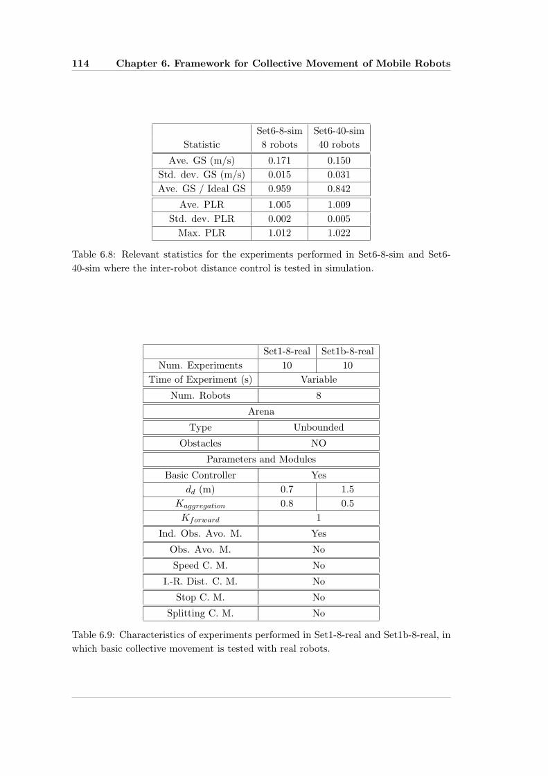
114 Chapter 6. Framework for Collective Movement of Mobile Robots
Set6-8-sim Set6-40-simStatistic 8 robots 40 robots
Ave. GS (m/s) 0.171 0.150Std. dev. GS (m/s) 0.015 0.031Ave. GS / Ideal GS 0.959 0.842
Ave. PLR 1.005 1.009Std. dev. PLR 0.002 0.005
Max. PLR 1.012 1.022
Table 6.8: Relevant statistics for the experiments performed in Set6-8-sim and Set6-40-sim where the inter-robot distance control is tested in simulation.
Set1-8-real Set1b-8-realNum. Experiments 10 10
Time of Experiment (s) Variable
Num. Robots 8
Arena
Type Unbounded
Obstacles NO
Parameters and Modules
Basic Controller Yesdd (m) 0.7 1.5
Kaggregation 0.8 0.5Kforward 1
Ind. Obs. Avo. M. Yes
Obs. Avo. M. No
Speed C. M. No
I.-R. Dist. C. M. No
Stop C. M. No
Splitting C. M. No
Table 6.9: Characteristics of experiments performed in Set1-8-real and Set1b-8-real, inwhich basic collective movement is tested with real robots.

6.5. Experiments with Real Robots 115
0 1 2 3 4 5 6 7 83
3.5
4
4.5
5
5.5
6
6.5
7
7.5
x [m]
y [m
]
(a) Trajectories of the robots during the experiment. The initial positions of the robots are marked
with a small circle, while the final positions are marked with a square
0 5 10 15 20 25 300
0.05
0.1
0.15
0.2
0.25
0.3
time [s]
spee
d [m
/s]
(b) GroupSpeed(t) for an experiment.
0 5 10 15 20 25 300.06
0.08
0.1
0.12
0.14
0.16
0.18
0.2
0.22
time [s]
mea
n di
stan
ce e
rror
[m]
(c) MeanDistanceError(t) for the same experi-
ment.
Figure 6.15: Relevant metrics and robots’ trajectories shown for a single experiment ofSet1-8-real tested with real robots.
116 Chapter 6. Framework for Collective Movement of Mobile Robots
5.56
6.57
7.58
8.59
2 3 4 5 6 7 8 9 10
x [m]
y [m]
(a) Trajectories of the robots during the experiment. The initial positions of the robots are marked
with a small circle, while the final positions are marked with a square
0 5 10 15 20 25 300
0.05
0.1
0.15
0.2
0.25
0.3
time [s]
spee
d [m
/s]
(b) GroupSpeed(t) for an experiment.
0 5 10 15 20 25 300.2
0.3
0.4
0.5
0.6
0.7
0.8
0.9
1
time [s]
mea
n di
stan
ce e
rror
[m]
(c) MeanDistanceError(t) for the same experi-
ment.
Figure 6.16: Relevant metrics and robots’ trajectories shown for a single experiment ofSet1b-8-real tested with real robots.
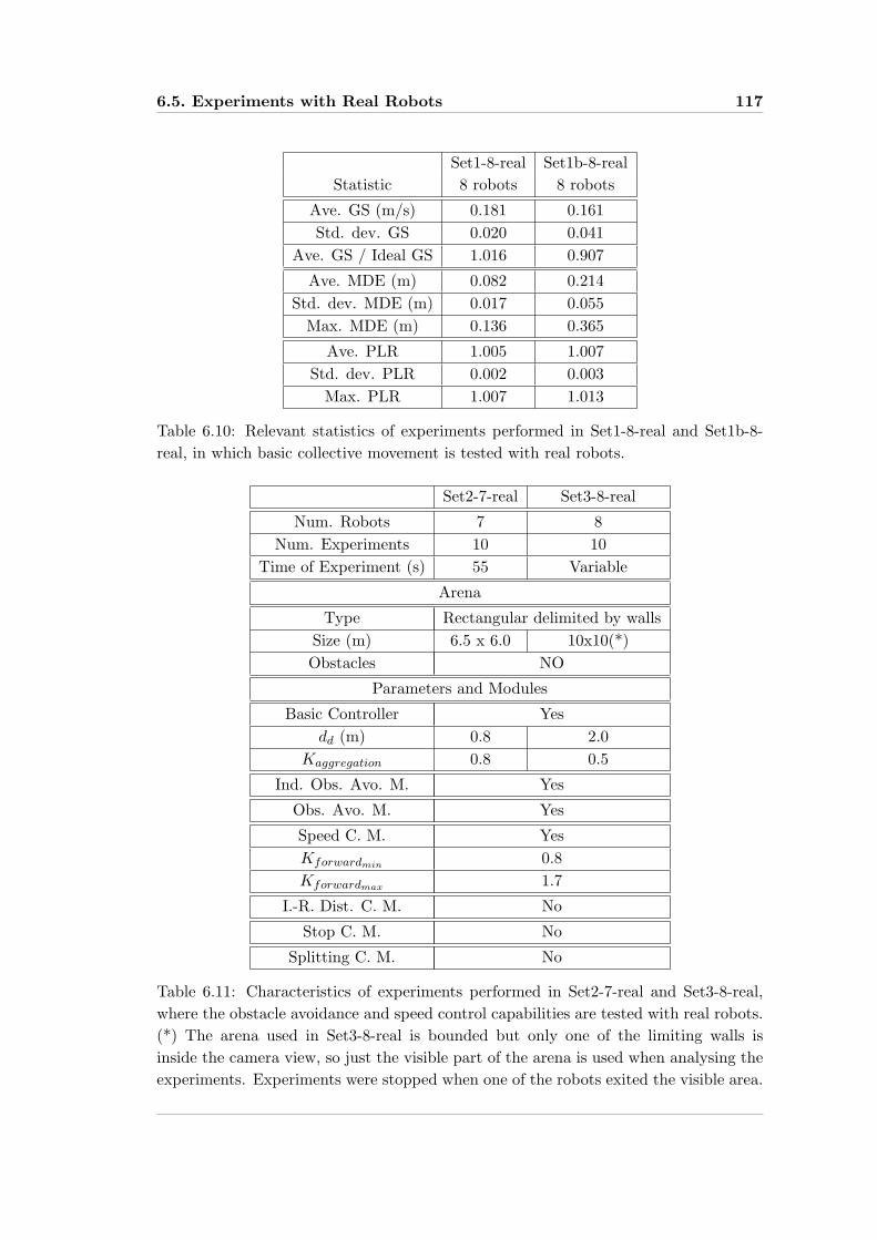
6.5. Experiments with Real Robots 117
Set1-8-real Set1b-8-realStatistic 8 robots 8 robots
Ave. GS (m/s) 0.181 0.161Std. dev. GS 0.020 0.041
Ave. GS / Ideal GS 1.016 0.907
Ave. MDE (m) 0.082 0.214Std. dev. MDE (m) 0.017 0.055
Max. MDE (m) 0.136 0.365
Ave. PLR 1.005 1.007Std. dev. PLR 0.002 0.003
Max. PLR 1.007 1.013
Table 6.10: Relevant statistics of experiments performed in Set1-8-real and Set1b-8-real, in which basic collective movement is tested with real robots.
Set2-7-real Set3-8-real
Num. Robots 7 8Num. Experiments 10 10
Time of Experiment (s) 55 Variable
Arena
Type Rectangular delimited by wallsSize (m) 6.5 x 6.0 10x10(*)Obstacles NO
Parameters and Modules
Basic Controller Yesdd (m) 0.8 2.0
Kaggregation 0.8 0.5
Ind. Obs. Avo. M. Yes
Obs. Avo. M. Yes
Speed C. M. YesKforwardmin 0.8Kforwardmax 1.7
I.-R. Dist. C. M. No
Stop C. M. No
Splitting C. M. No
Table 6.11: Characteristics of experiments performed in Set2-7-real and Set3-8-real,where the obstacle avoidance and speed control capabilities are tested with real robots.(*) The arena used in Set3-8-real is bounded but only one of the limiting walls isinside the camera view, so just the visible part of the arena is used when analysing theexperiments. Experiments were stopped when one of the robots exited the visible area.

118 Chapter 6. Framework for Collective Movement of Mobile Robots
they reduce velocity because an obstacle is detected (probably wall at x = 9, 05m).After avoiding the two firs wall, at t = 40 s there is another acceleration, followed bya decrease of speed since wall at y = 1.46 m is perceived. The high peaks in velocitycorrespond with large MDO as can be seen in Figure 6.18(c). MDE is plotted withtime in Figure 6.18(b).
44.5
55.5
66.5
77.5
88.5
92 3 4 5 6 7 8
x [m]
y [m]
Figure 6.17: Trajectories of the robots during an experiment of Set2-8-real whereobstacle avoidance and speed control are tested with real robots. The initial positionsof the robots are marked with a small circle, while the final positions are marked witha square.
In Table 6.12, relevant statistics of experiments performed in Set2-7-real and Set3-8-real are shown. They are calculated for each set of experiments for all the experimentsfor t > 5 s. The results are very similar to the comparable cases in simulation (Set2-7-sim and Set3-8-sim). The main difference is PPTCO for Set3-8-real, that is 0 in everycase. The security distance used is sc = 0.05 m, similar to the error introduced by thetracking system, so it might be the reason for PPTCO = 0. In addition, robots do notreach a wall in every experiment, being stopped when exit the tracking area.
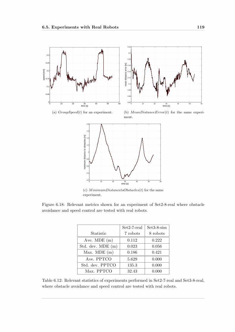
6.5. Experiments with Real Robots 119
0 10 20 30 40 50 600
0.05
0.1
0.15
0.2
0.25
0.3
time [s]
spee
d [m
/s]
(a) GroupSpeed(t) for an experiment.
0 10 20 30 40 50 600.04
0.06
0.08
0.1
0.12
0.14
0.16
0.18
0.2
0.22
time [s]
mea
n di
stan
ce e
rror
[m]
(b) MeanDistanceError(t) for the same experi-
ment.
0 10 20 30 40 50 600.2
0.4
0.6
0.8
1
1.2
1.4
1.6
1.8
time [s]
min
imum
dis
tanc
e to
obs
tacl
es [m
]
(c) MinimumDistancetoObstacles(t) for the same
experiment.
Figure 6.18: Relevant metrics shown for an experiment of Set2-8-real where obstacleavoidance and speed control are tested with real robots.
Set2-7-real Set3-8-simStatistic 7 robots 8 robots
Ave. MDE (m) 0.112 0.222Std. dev. MDE (m) 0.023 0.056
Max. MDE (m) 0.186 0.421
Ave. PPTCO 5.629 0.000Std. dev. PPTCO 135.3 0.000
Max. PPTCO 32.43 0.000
Table 6.12: Relevant statistics of experiments performed in Set2-7-real and Set3-8-real,where obstacle avoidance and speed control are tested with real robots.
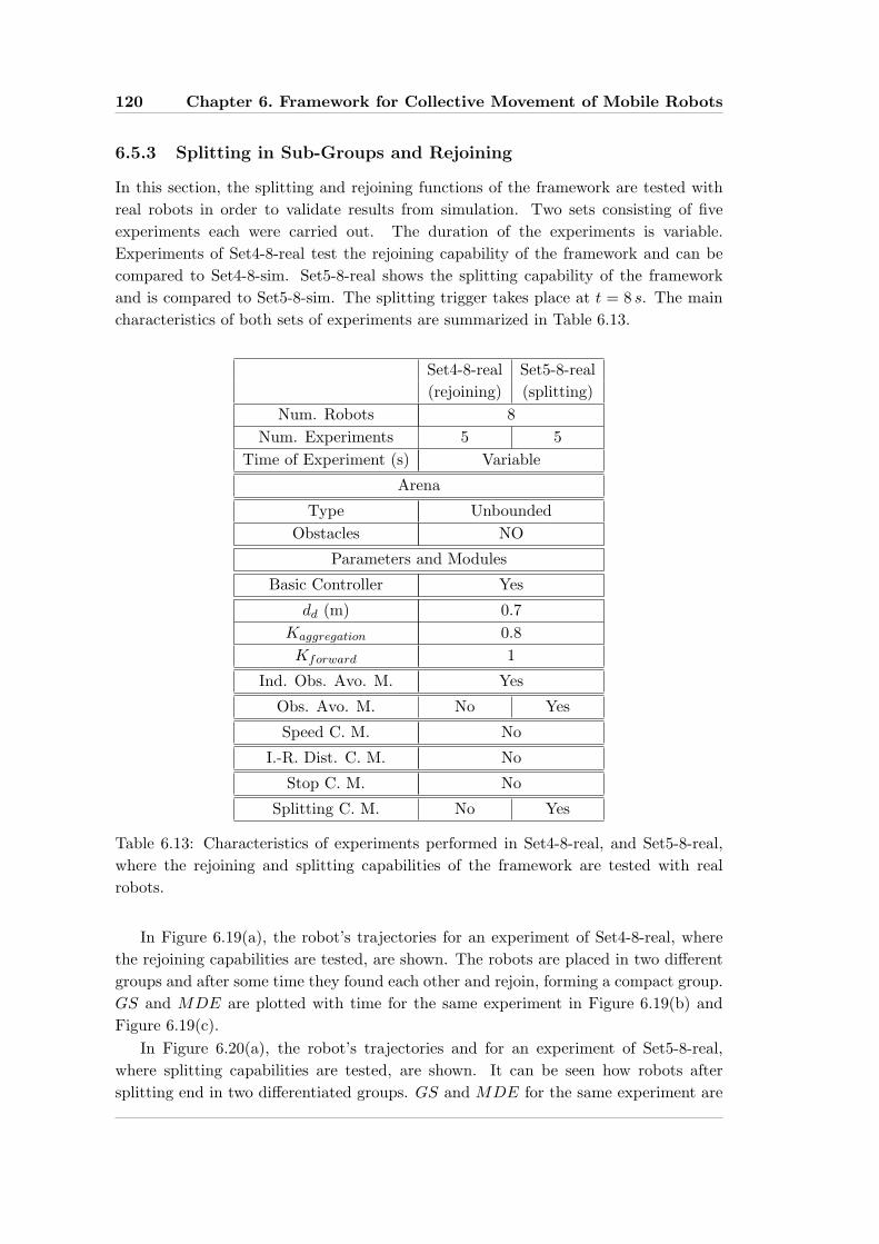
120 Chapter 6. Framework for Collective Movement of Mobile Robots
6.5.3 Splitting in Sub-Groups and Rejoining
In this section, the splitting and rejoining functions of the framework are tested withreal robots in order to validate results from simulation. Two sets consisting of fiveexperiments each were carried out. The duration of the experiments is variable.Experiments of Set4-8-real test the rejoining capability of the framework and can becompared to Set4-8-sim. Set5-8-real shows the splitting capability of the frameworkand is compared to Set5-8-sim. The splitting trigger takes place at t = 8 s. The maincharacteristics of both sets of experiments are summarized in Table 6.13.
Set4-8-real Set5-8-real(rejoining) (splitting)
Num. Robots 8Num. Experiments 5 5
Time of Experiment (s) Variable
Arena
Type UnboundedObstacles NO
Parameters and Modules
Basic Controller Yes
dd (m) 0.7Kaggregation 0.8Kforward 1
Ind. Obs. Avo. M. Yes
Obs. Avo. M. No Yes
Speed C. M. No
I.-R. Dist. C. M. No
Stop C. M. No
Splitting C. M. No Yes
Table 6.13: Characteristics of experiments performed in Set4-8-real, and Set5-8-real,where the rejoining and splitting capabilities of the framework are tested with realrobots.
In Figure 6.19(a), the robot’s trajectories for an experiment of Set4-8-real, wherethe rejoining capabilities are tested, are shown. The robots are placed in two differentgroups and after some time they found each other and rejoin, forming a compact group.GS and MDE are plotted with time for the same experiment in Figure 6.19(b) andFigure 6.19(c).
In Figure 6.20(a), the robot’s trajectories and for an experiment of Set5-8-real,where splitting capabilities are tested, are shown. It can be seen how robots aftersplitting end in two differentiated groups. GS and MDE for the same experiment are
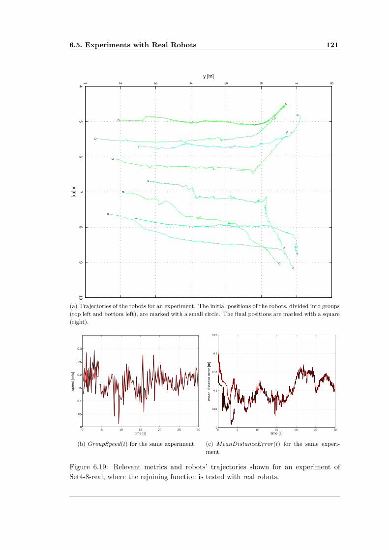
6.5. Experiments with Real Robots 121
45
67
89
101 2 3 4 5 6 7 8
x [m]
y [m]
(a) Trajectories of the robots for an experiment. The initial positions of the robots, divided into groups
(top left and bottom left), are marked with a small circle. The final positions are marked with a square
(right).
0 5 10 15 20 25 300
0.05
0.1
0.15
0.2
0.25
0.3
time [s]
spee
d [m
/s]
(b) GroupSpeed(t) for the same experiment.
0 5 10 15 20 25 300
0.05
0.1
0.15
0.2
0.25
time [s]
mea
n di
stan
ce e
rror
[m]
(c) MeanDistanceError(t) for the same experi-
ment.
Figure 6.19: Relevant metrics and robots’ trajectories shown for an experiment ofSet4-8-real, where the rejoining function is tested with real robots.
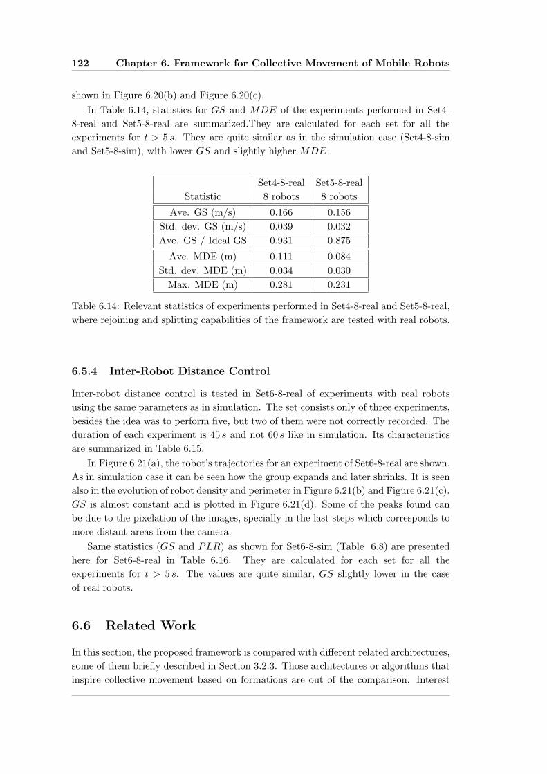
122 Chapter 6. Framework for Collective Movement of Mobile Robots
shown in Figure 6.20(b) and Figure 6.20(c).In Table 6.14, statistics for GS and MDE of the experiments performed in Set4-
8-real and Set5-8-real are summarized.They are calculated for each set for all theexperiments for t > 5 s. They are quite similar as in the simulation case (Set4-8-simand Set5-8-sim), with lower GS and slightly higher MDE.
Set4-8-real Set5-8-realStatistic 8 robots 8 robots
Ave. GS (m/s) 0.166 0.156Std. dev. GS (m/s) 0.039 0.032Ave. GS / Ideal GS 0.931 0.875
Ave. MDE (m) 0.111 0.084Std. dev. MDE (m) 0.034 0.030
Max. MDE (m) 0.281 0.231
Table 6.14: Relevant statistics of experiments performed in Set4-8-real and Set5-8-real,where rejoining and splitting capabilities of the framework are tested with real robots.
6.5.4 Inter-Robot Distance Control
Inter-robot distance control is tested in Set6-8-real of experiments with real robotsusing the same parameters as in simulation. The set consists only of three experiments,besides the idea was to perform five, but two of them were not correctly recorded. Theduration of each experiment is 45 s and not 60 s like in simulation. Its characteristicsare summarized in Table 6.15.
In Figure 6.21(a), the robot’s trajectories for an experiment of Set6-8-real are shown.As in simulation case it can be seen how the group expands and later shrinks. It is seenalso in the evolution of robot density and perimeter in Figure 6.21(b) and Figure 6.21(c).GS is almost constant and is plotted in Figure 6.21(d). Some of the peaks found canbe due to the pixelation of the images, specially in the last steps which corresponds tomore distant areas from the camera.
Same statistics (GS and PLR) as shown for Set6-8-sim (Table 6.8) are presentedhere for Set6-8-real in Table 6.16. They are calculated for each set for all theexperiments for t > 5 s. The values are quite similar, GS slightly lower in the caseof real robots.
6.6 Related Work
In this section, the proposed framework is compared with different related architectures,some of them briefly described in Section 3.2.3. Those architectures or algorithms thatinspire collective movement based on formations are out of the comparison. Interest

6.6. Related Work 123
45
67
89
103 4 5 6 7 8 9 10
x [m]
y [m]
(a) Trajectories of the robots during an experiment. The initial positions of the robots are marked
with a small circle (right). The final positions, where robots are split into two groups (top left and
bottom left) are marked with a square.
0 5 10 15 20 25 30 35 400
0.05
0.1
0.15
0.2
0.25
0.3
time [s]
spee
d [m
/s]
(b) GroupSpeed(t) for the same experiment.
0 5 10 15 20 25 30 35 400.02
0.04
0.06
0.08
0.1
0.12
0.14
0.16
0.18
0.2
time [s]
mea
n di
stan
ce e
rror
[m]
(c) MeanDistanceError(t) for the same experi-
ment.
Figure 6.20: Relevant metrics and robots’ trajectories shown for an experiment ofSet5-40-real, where the splitting function is tested with real robots.

124 Chapter 6. Framework for Collective Movement of Mobile Robots
Set6-8-realNum. Robots 8
Num. Experiments 3Time of Experiment (s) 45
Arena
Type Unbounded
Obstacles NO
Parameters and Modules
Basic Controller YesKaggregation 0.8Kforward 1
Ind. Obs. Avo. M. Yes
Obs. Avo. M. No
Speed C. M. No
I.-R. Dist. C. M. Yesfunction Sinusoidal
period (s) 45ddmin (m) 0.5ddmax (m) 1.5
Stop C. M. No
Splitting C. M. No
Table 6.15: Characteristics of experiments carried out in Set6-8-real where the inter-robot distance control is tested with real robots.
Set6-8-simStatistic 8 robots
Ave. GS (m/s) 0.156Std. dev. GS (m/s) 0.031Ave. GS / Ideal GS 0.875
Ave. PLR 1.011Std. dev. PLR 0.001
Max. PLR 1.013
Table 6.16: Relevant statistics for the experiments carried out in Set6-8-real where theinter-robot distance control is tested with real robots.
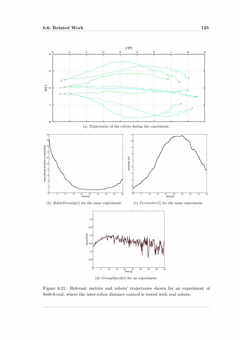
6.6. Related Work 125
45
67
80 1 2 3 4 5 6 7 8 9
x [m]
y [m]
(a) Trajectories of the robots during the experiment.
0 5 10 15 20 25 30 35 40 450
2
4
6
8
10
12
14
16
18
20
time [s]
robo
t den
sity
[num
ber
of r
obot
s/m
2]
(b) RobotDensity(t) for the same experiment.
0 5 10 15 20 25 30 35 40 452
3
4
5
6
7
8
9
10
11
time [s]
perim
eter
[m]
(c) Perimeter(t) for the same experiment.
0 5 10 15 20 25 30 35 40 450
0.05
0.1
0.15
0.2
0.25
0.3
time [s]
spee
d [m
/s]
(d) GroupSpeed(t) for an experiment.
Figure 6.21: Relevant metrics and robots’ trajectories shown for an experiment ofSet6-8-real, where the inter-robot distance control is tested with real robots.

126 Chapter 6. Framework for Collective Movement of Mobile Robots
is given to those more focused on flocking and lattice based structures, and which arescalable with increasing number of robots.
The Basic Controller used in the framework is based on the combination of twovectors representing the direction and speed of the group (~vi,group) and the aggregationbetween robots (~vi,aggregation). These vectors are weighted and summed working in avery similar way as motor-schemas do in Balch (1998). In our framework the resultingvector is converted into motor speeds to create collective movement and to distributerobots in a triangular lattice, while in Balch (1998) formations with different structuresare created.
Lee and Chong (2009) propose a formation algorithm that needs a completecoordinate system. As it is explained in Section 3.2.3, in order to create this coordinatesystem every robot should be aware of the relative positions of every other robot in thegroup. The proposed common orientation agreement method used in our frameworkis not limited in that way and it is scalable with increasing number of robots. Itonly maintains orientation information and does not give any translation information.But, as said in Section 5.7, the algorithm could be easily augmented to track x and y
coordinated.The framework uses, depending on the modules, several consensus algorithms in
order to agree on the direction of movement, speed and inter-robot distance. Severalresearchers use consensus algorithms in their controllers in order to make all the robotsagree in a common velocity. This is the case of Tanner et al. (2003a,b,c), where robotagree on the velocity in order to create flocking movement. The algorithm needsthat robots know the relative velocities of the neighboring robots, which is difficultto estimate using real robots. In addition, the consensus algorithm is based on theaverage of the own velocity and neighboring robots’ velocities, without weighting them,giving the same importance to every robot information. Olfati-Saber (2006) also makesuse of a consensus algorithm that agrees on the velocities of the robots, in order tocreate collective movement and place robots forming triangular lattices. This timethe influence of neighboring robots’ velocities on the calculation of the new velocityis weighted, depending on a weighting factor that is function of the distance betweenrobots. The architecture also assumes that velocities of neighboring robots are known.In addition, these architectures based on consensus algorithms are usually only testedin simulation. Their implementation on real robots can be quite difficult due to thedifficulty of determining the velocities of neighboring robots.
The main differences and advantages of our framework compared to Tanner et al.(2003a,b,c) and Olfati-Saber (2006) are the following:
• It is not necessary to estimate the velocities of neighboring robots since robotsshare a common orientation reference and share their velocities referred to itusing wireless communication. This common orientation reference is calculatedalso based on a consensus algorithm, but does not need to estimate velocities,only positions of neighboring robots.
• The consensus algorithms calculate the resulting variables as a weighted sum of

6.6. Related Work 127
the own variables and those of its neighboring robots. This weight represents theimportance of the information given by the agent, for instance allowing robots inthe presence of an obstacle to have more influence into his neighbors. In addition,this weight or influence is propagated over the network allowing fast changes inthe variables.
• Since robots use their consensus agreement based on variables obtained bycommunication, and not by observation, the convergence can be faster. In theobservation case a robot changing its heading starts influencing its neighborsto change their headings once it has turned, which takes some time. By usingcommunication the consensus algorithms speed up, since information is availableto neighbors only with the delay of communications latency.
• Consensus algorithms are not only applied to the velocity, but also to othervariables like inter-robot distance.
The Physicomimetics Framework (PF) (Spears et al., 2004b,a, 2005), allows creationof triangular lattices based on a fully decentralized algorithm. As in our framework,robots react to the neighboring positions with attractive or repulsive forces, but theyneed global information to move towards and objective. PF is scalable with increasingnumber of robots, as it is shown in simulations. In PF, robots are considered tobe holonomic vehicles. Its use in non-holonimic robots is done by performing arotational movement followed by a translational one within a large time window.However, such a workaround would not be practical for most of the potential real-world applications. On real robots, the goal to follow is a bright light. Lee andChong (2008b) propose a distributed and scalable algorithm for collective movement, inwhich robots position themselves creating a triangular lattice, similar to our proposedframework. Its convergence is proved using Lyapunov’s theorem. As in PF, robots areattracted by a virtual (stationary or moving) goal in order to create group movement.It is tested only in simulation, with up to 100 robots. No results using real robotsare shown. In Lindhe and Johansson (2005) and Lindhe and Ogren (2005) a similardecentralized algorithm based on lattice formations is presented. As in Lee and Chong(2008b), robots need to know the position of a goal in order to inspire movement.The stability is studied and experiments are performed only in simulation, with noexperiments using real robots. Antonelli et al. (2008) propose a method based in theNull-Space-based Behavioral (NSB) control (Antonelli et al., 2010), that also createscollective movement placing robots in a triangular lattice. It also needs a virtual goalwhich limits the scalability and application on real robots. The method is tested insimulation and also on real robots. The control of real robots if performed off-board,using a camera that tracks the positions of the robots, and sending commands to themotors. Our proposed framework does not need to know the position of a virtualgoal, and direction of movement is decided between all the robots, without the need ofany external global reference thanks to the common orientation consensus algorithm.This allows to implement the algorithm on real robots, without the need of special

128 Chapter 6. Framework for Collective Movement of Mobile Robots
solutions, such as the use of intense light in the case of PF, or indicating the goal byusing a camera system in the case of NSB.
In Hayes and Dormiani-Tabatabaei (2002) a distributed algorithm for flocking ofrobots is presented. Robots do not need to know the velocities of neighbors or followa virtual goal. Direction of movement is calculated using the variation of the centerof mass of neighboring robots between two time steps. Validation of the algorithm iscomplemented using 10 real robots provided with emulated estimation of neighboringrobots’ positions, using an external tracking system. The algorithm represents oneof the initial works of flocking where a scalable algorithm and real robots are used.The main advantage of our framework compared to this algorithm is that faster andmore intelligent changes or agreements in the direction of movement can be done. Inaddition, in our case more regular patterns are formed.
Turgut et al. (2008) present a scalable and distributed algorithm for robot flocking.It is based on the heading alignment of the robots and the inter-robot distance control.Robots are provided with a compass and with wireless communications so that they caninform their neighbors of their heading with respect to their detected magnetic north.The algorithm is tested in simulation with hundreds robots and with a small groupof real robots. The use of a compass provides robots with the same information thatresults in our framework of applying the common orientation agreement algorithm. Theproblems resulting from using a compass are summarized in Section 5.1. The alignmentof the robots’ heading is based on the robots’ heading and not on a desired heading, asin the case of our framework. This makes this slower towards changes in the directionof movement, and does not allow to give more importance to the heading of a robot incase its direction of movement would have more priority.
6.7 Conclusions
In this chapter, a framework for the collective movement of mobile robots has beenproposed, analyzed and tested. It allows robots to move as a unique entity, agree in thegroup velocity, avoid obstacles by changing the group direction of movement, modifythe inter-robot distance, split the group into sub-groups and rejoin different groups intoa larger one.
The controller is distributed among the robots and makes use of the consensusalgorithms described in Chapter 5, which allow the robots to agree on a distributedfashion on a common orientation reference. This controller allows the group of robotsto move in a common direction, imposing an inter-robot distance between the robots,by the robots reacting to the positions of their neighbors. The positions of robots forma triangular lattice. The way neighboring robots are chosen, specifically those of type2, means an innovation compared to other collective movement architectures based onNeighbor-referenced algorithms. It allows the group of robots to be more compact, itprevents robots from separating from the group unnecessarily, and it helps differentgroups of robots rejoin into a larger one if it is necessary.
The framework is composed of different modules that modify the behavior of the
6.8. Future Work 129
group allowing different movement functions. Most of them are based on a consensusalgorithm that allows the robots to agree on different parameters and also to imposeits value to the rest when they have relevant information. The consensus algorithmsused in the different modules are very similar in their workings and implementationand can be used as a starting point to develop new modules.
The consensus algorithms for agreement on the group velocity (speed and direction)together with the common orientation agreement algorithm, avoid using an externalobjective towards which to move the robots and relieve them from estimating thevelocities or headings of neighboring robots. An external objective is used in manycollective movement algorithms, making the algorithm not scalable since every robotmust know the position of the objective. In addition, it is not practical for real roboticapplications. The estimation of neighboring robots’ velocities or headings is used inmost of the collective movement algorithms based on consensus. Estimating velocitieson real robots is difficult.
The use of consensus algorithms based on the communication of the variables underagreement together with the propagation of the weighting values of those variables maketheir convergence faster than if they were based on the observation of the variables,and allow a fast propagation over the network of robots that permits the scalabilitywith an increasing number of robots.
The framework can be expanded with new modules in order to implement newcapabilities. These modules can be based on consensus algorithms as most of theproposed modules or can be implemented in a different way. These new modules canimplement more complicated tasks such as search or mapping.
The proposed framework can be implemented on any mobile robot capable ofestimating the relative positions of nearby robots and communicating with them. Ifthe kinematics of the robots differ from differential drive configuration new low levelcontrollers should be implemented.
The framework has been successfully tested in simulation and using real robots.Experiments with real robots were carried out using eight Khepera III robots,demonstrating that the framework works correctly in reality. In simulation, up to40 Khepera III robots were used, demonstrating experimentally the scalability with anincreasing number of robots.
6.8 Future Work
The proposed framework can be augmented by adding new modules or by developingsome of the already described ones to increase their autonomy.
The Inter-Robot Distance Control Module can be modified to change the inter-robot desired distance according to external events. Checking the continuous presenceof obstacles in different points of the group might indicate that the group is passinga corridor. This can be detected collectively in a distributed manner. If a corridoris detected robots can agree on a lower inter-robot-distance for an easier movementthrough the corridor.
130 Chapter 6. Framework for Collective Movement of Mobile Robots
The Splitting Control Module can be augmented to decide when and in which placeof the group the splitting should take place. This must be done according to theinformation read by the robot’s sensors and shared among them. The decision can bedone in a distributed manner, maybe making use of a consensus algorithm.
A distributed search mechanism (of odor or sound) could be implemented by addinga module based on a consensus algorithm that would change the desired group directionof movement depending on the measures obtained by each robot and its neighbors.
A module for changing the external shape of the group of robots can beimplemented. External robots might detect if they are in the border of the groupand try to modify their positions to change the external shape.
The framework could be augmented to cope with movement in three dimensions.The basic workings of the framework would be the same. The Basic Controller shouldbe modified to allow 3-dimensional vectors and new low level controllers should beimplemented depending on the robots used. The robots used to test the algorithmcould be aerial or underwater vehicles. The consensus algorithm for agreement on acommon reference should be augmented to the three angles present in a 3-dimensionalpose. New different modules in charge of modifying some of the parameters of the newBasic Controller should be implemented, especially those in charge of changing thedirection of movement, like the Obstacle Avoidance Module. The Inter-Robot DistanceControl Module and the Speed Control Module could be directly reused without anychanges or just minor ones.

Part III
Conclusions

Chapter 7
Conclusions and Future Work
The best way to predict the future is to invent it.
Alan Kay - Stanford Engineering, Volume 1, Number 1, Autumn 1989.
7.1 Introduction
In this Thesis, a framework for the control of collective movement of mobile robots hasbeen designed, presented and analysed. It makes use of a distributed algorithm (alsoproposed in this Thesis) for the consensus on an orientation reference. In addition, aset of metrics for the analysis of collective movement of robots has been designed andimplemented in order to analyze the performance of the framework and the consensusalgorithm. The conclusions obtained in these three areas are explained in Section 7.2,while future lines of work are summarized in Section 7.3.
7.2 Conclusions
The proposed framework for collective movement of mobile robots allows robots tomove as a unique entity. Robots agree in the group velocity, are able to avoid obstaclesby changing the group direction of movement in a distributed fashion, and modify theinter-robot distance. Moreover, they can split the group into sub-groups and rejoindifferent groups into a larger one.
The controller underlying the framework is distributed among the robots and itmakes use of the consensus algorithm for agreement on a common orientation reference,also designed and explained in this Thesis. This controller allows the group of robotsto move in a common direction and impose an inter-robot distance, by making robotsmove according to the neighbors’ positions. The positions of robots form a triangularlattice. The way neighboring robots are chosen, concretely the distinction of two typesof neighboring robots, means an innovation compared to other collective movementarchitectures based on Neighbor-referenced algorithms. It allows the group of robotsto be more compact and avoids that robots separate from the group unnecessarily. Itallows different groups of robots to rejoin into a larger one.
134 Chapter 7. Conclusions and Future Work
The framework is composed of different modules that modify the behavior of thegroup allowing different movement functions. Most of them are based on a consensusalgorithm that allows the robots to agree on different parameters and to impose itsvalue to the rest when they have relevant information. The consensus algorithms usedin the different modules are very similar in their workings and implementation and canbe used as starting point to develop new modules.
The consensus algorithms for the agreement on the group direction combined withthe common orientation agreement algorithm avoid the use of an external objective andrelieve the robots from knowing the velocities or headings of their neighbors. Manycollective movement algorithms, specially those based on attractive/repulsive functions,need an external objective in order to move in a certain direction. This makes thealgorithm not scalable since every robot needs to know the position of the objective,and hence not practical for real robotic applications. The estimation of neighboringrobots’ velocities or headings is also necessary in many algorithms based on consensus.This estimation is difficult with real robots.
Consensus algorithms based on the communication of the variables under agreementtogether with the propagation of the weighting values of those variables, make theirconvergence faster than if they were based on the observation of the variables. Theyalso allow a fast propagation over the network of robots, which helps to allow thescalability with an increasing number of robots.
New modules can be designed in order to implement new capabilities. They can bebased on consensus algorithms as most of the proposed modules or can be implementedin a different manner. These new modules can implement more complicated tasks suchas search or mapping.
The framework can be easily implemented on any mobile robot capable of measuringthe relative positions of neighboring robots and communicating with them. If therobots do not have differential drive configuration new low level controllers should beimplemented taking into account their kinematics.
The framework has been successfully tested in simulation and using real robots.Experiments with real robots were carried out using eight Khepera III robots,demonstrating that the framework works correctly in reality. Many of the roboticcollective movement architectures developed up to date are not tested on real robots,or sometimes real robots are used but by emulating some sensors (relative positioningsystems, position of an objective), so successfully carrying out real experimentsrepresents an advance. In simulation experiments, up to 40 Khepera III robots wereused, demonstrating experimentally the scalability with an increasing number of robots.
As it has been said, the framework uses an algorithm that makes robots agree ona reference orientation. This algorithm has been explained and analyzed in the Thesisand represents also a contribution by providing robots with a reference orientation thatis obtained in a distributed and scalable way.
This consensus algorithm for agreement on orientation just needs that robots possessa relative positioning system, capable of detecting the positions of nearby robots, and alocal communication system. Two different consensus algorithms based on the exchange
7.3. Future Work 135
of information were proposed, tested and analyzed.In order to test the method, systematic experiments were carried out in simulation
and with real robots, varying the consensus algorithm, the α parameter of the consensusalgorithm, and the communication topology. CAA consensus algorithm did notconverge in every experiment when robots were placed in ring topology. Successdepended on the initial conditions. On the other hand, CAB converged in everyexperiment for all the set of experiments run. Its convergence has not been provedmathematically, but experimental results allow to trust the use of the algorithm. Atotal of 310 experiments 60 s duration were performed: 270 of them in simulation andthe remaining 40 using real robots.
Scalability with an increasing number of robots was tested successfully in simulationwith up to 49 robots. All experiments with real robots succeeded in proving that theproposed method works in reality. Experiments with a large group of real robots werenot carried out, but the mentioned scalability in simulation seems to indicate that itwould work properly.
The method assumes synchronicity of the robots’ clocks. Experiments in simulationwith delays among the robots’ clocks introduced on purpose, and experiments with realrobots in which there exists no perfect synchronicity, revealed that the algorithmsworked properly, with convergence to the reference orientation for all the robots.However, these values do not always keep stable, varying slowly with time. Themaximum variation measured was 0.01 rad/s.
One of the advantages of this method is that if robots already posses a systemfor estimating the relative position of nearby robots, there is no need for new specifichardware. In principle, the algorithm could work on any robot capable of detecting theposition of other robots and communicating with them.
In order to analyze the performance of the framework a set of metrics for collectivemovement was defined and briefly discussed. Some of the metrics are useful just tocharacterize the algorithms while others can be used to compare their performance.
Some of the metrics depend on arbitrary parameters which could make thecomparison between different algorithms difficult. Moreover, in order to be able tocompare different algorithms, it is necessary not only to have a set of metrics but toshare a common set of environments with obstacles and places that groups of robotsmust reach.
7.3 Future Work
The framework presented in the Thesis can be augmented by adding new modules orby developing some of the already described ones to increase their autonomy.
The Inter-Robot Distance Control Module can be modified to change the inter-robotdesired distance according to external events. For instance, checking the continuouspresence of obstacles in different points of the group might indicate that the group ispassing a corridor.
The Splitting Control Module can be augmented to decide when and where in the
136 Chapter 7. Conclusions and Future Work
group the splitting will take place. This must be done according to the informationread by the robot’s sensors and shared among them.
Distributed search (of odor or sound) could be implemented by adding a modulebased on a consensus algorithm that would change the desired group direction ofmovement depending on the measures acquired by each robot and its neighbors.
A module for changing the external shape of the group of robots can beimplemented. External robots might detect if they are on the border of the groupand try to modify their positions to change the external shape.
The framework can be augmented to cope with movement in three dimensions. Inprinciple, the workings of the framework would be the same. The controller shouldbe modified to allow 3-dimensional vectors and new low level controllers should beimplemented. The robots used to test the algorithm could be aerial or underwatervehicles. The consensus algorithm for agreement on a common reference should beredesigned to agree on the three angles present in a 3-dimensional pose. New differentmodules in charge of modifying some of the parameters of the controller should beimplemented, specially those in charge of changing the direction of movement. On theother hand, the Inter-Robot Distance Control Module and the Speed Control Modulecould be directly reused without any changes or only minor ones.
The method for distributed agreement on an orientation can be augmented and alsostudied more deeply. It is important to study rigorously the convergence of the CABalgorithm and, if necessary, modify it to ensure its convergence.
The algorithm could be modified to make it adaptive, being able to change the α
parameter, having a higher value in the beginning for a fast convergence, and a smallerone later on for more accuracy.
It would be also important to study what would happen if two different groupsof robots gather at a certain moment, since the confidences ci of all of them would bealready set to 1. One possible solution is that one of the groups had a higher confidencevalue than the other and would impose its reference orientation to the other.
The method could also be complemented by adding an origin point (0, 0), which willimply to have a complete coordinate system. Robots would need to keep track of thecomplete odometry (not only θ), and also to exchange messages with this informationand relative distances among them. Probably Kalman filters or a similar algorithmwould help in its implementation.

Part IV
Appendix


Appendix A
Experimental Platform
Quemadmodum gladius neminem occidit, occidentis telum est. (A swordnever kills anybody; it is a tool in the killer’s hand).
Lucius Annaeus Seneca
In this appendix, we present the tools and platforms used in the experiments thatserve to validate the algorithms proposed in the Thesis.
A.1 The Khepera III Robot Platform
The Khepera III is the mobile robot platform used for the validation of the Thesis. Itproduced by K-Team Corporation 1 (Pugh et al., 2009). Khepera III are small wheeledcylindrical robots, 12 cm in diameter, equipped with a variety of sensors, and whosemobility is ensured by a differential drive system using two independent motors. Themaximum speed of the robot is about 22 cm/s. It possesses a ring of 9 infrared sensorsfor very short range (3 cm) collision detection, as well as 5 middle range ultrasoundsensors. It is equipped with the Korebot platform, also developed by K-Team, runninga standard embedded Linux operating system on an Intel XSCALE PXA-255 processorrunning at 400 MHz. It has an expansion bus that allows adding new modules. It hastwo wireless communication systems: Bluetooth and IEEE 802.11 by using a card withits built-in CompactFlash slot. A picture of a Khepera III can be seen in Figure A.1
Khepera III robots are programmed and interacted easily using the KheperaIII Toolbox (Lochmatter, a) developed by the Distributed Intelligent Systems andAlgorithms Laboratory (DISAL) 2 at the Ecole Polytechnique Federale de Lausanne(EPFL). Khepera III Toolbox is described by its authors as a Swiss Army Knife for theKhepera III robot, offering three different types of tools: scripts to interact with therobots, small programs for the robots, and modules with standard functionality.
1K-Team website: http://www.k-team.com2DISAL website http://www5.epfl.ch/swis/

140 Chapter A. Experimental Platform
Figure A.1: A Khepera III robot.
A.1.1 Khepera III Relative Positioning System
In order to coordinate the robotic collective movement robots might know the positionsof the different robots. This can be done by using an external centralized system whichinforms robots of their positions and their neighbors’ positions. This situation is notalways possible in real environments and it is not fully scalable. Another possibilityis to use an on-board relative system, which allows robots to estimate the relativepositions of their neighboring robots.
This last solution is the used in the experiments performed in the Thesis. A relativepositioning system (Pugh et al., 2009), designed for Khepera III robots based oninfrared communications and developed by DISAL was used. The boards, pluggedon top of the robots, allow nearby robots to determine the range, bearing, andmessage of the sender with a rapid update rate using high-frequency modulated infraredemissions. Each robot emits packets to their neighboring robots using a ring of 16infrared sensors, using Carrier Sense Multiple Access (CSMA) communication protocolto avoid communication collisions. Each packet is emitted in less than 2 ms andconsists on 1 byte of overhead and 2 bytes of communication data. Modules that arenot emitting receive the emitted information and Received Signal Strength Indication(RSSI) through a ring of 8 receivers. Using RSSI values of the different receivers theyestimate both range and bearing to their nearby robots. The range of the boards is3.3meters. In Figure A.2 a relative positioning board can be seen.
A.2 Webots Robotic Simulator
It is necessary to use a robotic simulator in order to test and develop the algorithmsunder study in the Thesis, for initial development but also for later adjustment andsystematic tests. The use of a simulator tool allows much faster work than using realrobots. In addition, due to the availability problem of having a set of more than 10real robots a simulator is needed when performing experiments with high number ofrobots.
From the different available simulators Webots (Michel, 2004) was chosen for several
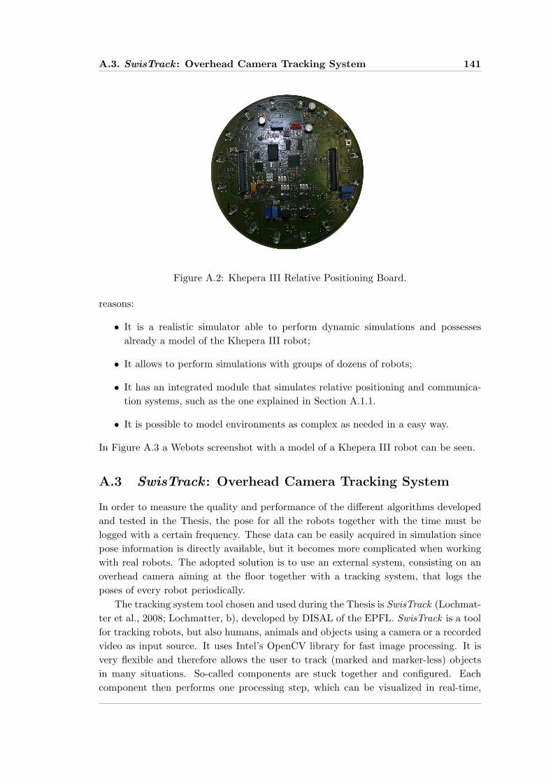
A.3. SwisTrack : Overhead Camera Tracking System 141
Figure A.2: Khepera III Relative Positioning Board.
reasons:
• It is a realistic simulator able to perform dynamic simulations and possessesalready a model of the Khepera III robot;
• It allows to perform simulations with groups of dozens of robots;
• It has an integrated module that simulates relative positioning and communica-tion systems, such as the one explained in Section A.1.1.
• It is possible to model environments as complex as needed in a easy way.
In Figure A.3 a Webots screenshot with a model of a Khepera III robot can be seen.
A.3 SwisTrack : Overhead Camera Tracking System
In order to measure the quality and performance of the different algorithms developedand tested in the Thesis, the pose for all the robots together with the time must belogged with a certain frequency. These data can be easily acquired in simulation sincepose information is directly available, but it becomes more complicated when workingwith real robots. The adopted solution is to use an external system, consisting on anoverhead camera aiming at the floor together with a tracking system, that logs theposes of every robot periodically.
The tracking system tool chosen and used during the Thesis is SwisTrack (Lochmat-ter et al., 2008; Lochmatter, b), developed by DISAL of the EPFL. SwisTrack is a toolfor tracking robots, but also humans, animals and objects using a camera or a recordedvideo as input source. It uses Intel’s OpenCV library for fast image processing. It isvery flexible and therefore allows the user to track (marked and marker-less) objectsin many situations. So-called components are stuck together and configured. Eachcomponent then performs one processing step, which can be visualized in real-time,

142 Chapter A. Experimental Platform
Figure A.3: A Webots window showing a Khepera III robot.
which it is quite useful for the set up of the system. SwisTrack is an open-sourceproject hosted on SourceForge.
Another possibility to get positioning information about the robots is to retrieve itdirectly from them. Relative positioning information of neighboring robots, combinedwith odometry, might be processed off-line in order to estimate the pose of each robotat a given time step. This solution was discarded since the use of an external trackingsystem is very easy to use once the camera and system has been settled and returnsdirect information.
Bibliography
Alanyali, M., Venkatesh, S., Savas, O., and Aeron, S. (2004). Distributed bayesianhypothesis testing in sensor networks. In Proceedings of the 2004 American ControlConference, volume 6, pages 5369– 5374.
Antonelli, G., Arrichiello, F., Chakraborti, S., and Chiaverini, S. (2007). Experiencesof formation control of multi-robot systems with the null-space-based behavioralcontrol. In Proceedings of the IEEE International Conference on Robotics andAutomation.
Antonelli, G., Arrichiello, F., and Chiaverini, S. (2008). Flocking for multi-robotsystems via the null-space-based behavioral control. In Proceedings of the IEEE/RSJInternational Conference on Intelligent Robots and Systems.
Antonelli, G., Arrichiello, F., and Chiaverini, S. (2010). The nsb control: a behavior-based approach for multi-robot systems. Paladyn, 1:48–56.
Arai, T., Pagello, E., and Parker, L. E. (2002). Editorial: Advances in multi-robotsystems. IEEE Transactions on Robotics and Automation, 18(5):655–661.
Arkin, R. C. (1998). Behavior-Based Robotics. MIT Press, Cambridge Massachusetts.
Bahgeci, E. and Sahin, E. (2005). Evolving aggregation behaviors for swarm roboticsystems: a systematic case study. In Proceedings 2005 IEEE Swarm IntelligenceSymposium, pages 333– 340.
Bajec, I. L., Zimic, N., and Mraz, M. (2005). Simulating flocks on the wing: The fuzzyapproach. Journal of Theoretical Biology, 233(2):199–220.
Balch, T. and Arkin, R. (1998). Behavior-based formation control for multi-robotteams. IEEE Transactions on Robotics and Automation, 14(6):926–939.
Balch, T. and Hybinette, M. (2000). Social potentials for scalable multi-robotformations. In IEEE International Conference on Robotics and Automation (ICRA’00), volume 1, pages 73 – 80.
Balch, T. R. (1998). Behavioral diversity in learning robot teams. PhD thesis, GeorgiaInstitute of Technology. Director-Ronald C. Arkin.

144 BIBLIOGRAPHY
Ballerini, M., Cabibbo, N., Candelier, R., Cavagna, A., Cisbani, E., Giardina, I.,Lecomte, V., Orlandi, A., Parisi, G., Procaccini, A., Viale, M., and Zdravkovic,V. (2008). Interaction ruling animal collective behavior depends on topologicalrather than metric distance: Evidence from a field study. Proceedings of the NationalAcademy of Sciences of the United States of America, 105(4):1232–1237.
Barfoot, T. D., christopher M. Clark, Rock, S. M., and D’Eleuterio, G. M. T. (2002).Kinematic pathe-planning for formations of mobile robots with a nonholonomicconstraint. In IROS.
Bauso, D., Giarre, L., and Pesenti, R. (2003). Distributed consensus protocols forcoordinating buyers. In Proceedings of the 42nd IEEE Conference on Decision andControl, volume 1, pages 588– 592, Maui, Hawaii.
Bayindir, L. and Sahin, E. (2007). A review of studies in swarm robotics. TurkishJournal of Electrical Engineering and Computer Sciences, 15:115–147.
Bazoula, A., Djouadi, M., and Maaref, H. . (2008). Formation control of multi-robotsvia fuzzy logic technique. International Journal of Computers, Communications andControl, III:179–184.
Beni, G. (2005). From swarm intelligence to swarm robotics. In Sahin, E. and Spears,W., editors, Swarm Robotics Workshop: State-of-the-art Survey, number 3342, pages1–9, Berlin Heidelberg. Springer-Verlag.
Bhatt, R., Tang, C. P., and Krovi, V. (2004). Geometric motion planning and formationoptimization for a fleet of nonholonomic wheeled mobile robots. In Proceedings ofthe 2004 IEEE International Conference on Robotics and Automation.
Bonabeau, E., Dorigo, M., and Theraulaz, G. (1999). Swarm Intelligence: From Naturalto Artificial Systems. Oxford University Press, New York, NY, USA.
Bonsignorio, F., Hallam, J., and del Pobil, A. P. GEM SIG review guidelines. Technicalreport, Euron GEM Sig.
Borenstein, J., Everett, H. R., and Feng, L. (1996). Where Am I? Systems and Methodsfor Mobile Robot Positioning. University of Michigan.
Braitenberg, V. (1984). Vehicles: Experiments in Synthetic Psychology. MIT Press.
Brooks, R. A. (1986). A robust layered control system for a mobile robot. IEEE Journalof Robotics and Automation, RA-2(1):2–27.
Cao, Y. U., Fukunaga, A. S., and Kahng, A. B. (1997). Cooperative mobile robotics:Antecedents and directions. Autonomous Robots, 4:226–234.
Caprari, G. and Siegwart, R. (2005). Mobile micro-robots ready to use: Alice.In Proceedings of IEEE/RSJ International Conference on Intelligent Robots andSystems, Canada.
BIBLIOGRAPHY 145
Carling, C., Svenson, P., Mrtenson, C., and Carlsen, H. (2003). A flock-based modelfor ad hoc communication networks. In Eight International Command and ControlResearch and Technology Symposium, Washington, DC, USA.
Celikkanat, H., Turgut, A. E., and Sahin, E. (2009). Distributed Autonomous RoboticSystems 8, chapter Guiding a Robot Flock via Informed Robots, pages 215–225.Springer Berlin Heidelberg.
Chaimowicz, L. and Kumar, V. (2004). Aerial shepherds: Coordination among uavsand swarms of robots. In 7th International Symposium on Distributed AutonomousRobotic Systems, ”Toulouse.
Chaimowicz, L., Michael, N., and Kumar, V. (2005). Controlling swarms of robotsusing interpolated implicit functions. In Proceedings of the 2005 IEEE InternationalConference on Robotics and Automation (ICRA 2005), pages 2487–2492.
Chang, C.-F. and Fu, L.-C. (2008). A formation control framework based on lyapunovapproach. In Proceedings of the IEEE/RSJ International Conference on IntelligentRobots and Systems.
Christensen, A., O’Grady, R., and Dorigo, M. (2007). Morphology control in amultirobot system. IEEE Robotics & Automation Magazine, 14(4):18–25.
Christensen, A. L., OGrady, R., and Dorigo, M. (2008). Swarmorph-script: a languagefor arbitrary morphology generation in self-assembling robots. Swarm Intelligence,2(2-4):143–165.
Chuang, Y.-L., Huang, Y., D’Orsogna, M., and Bertozzi, A. (2007). Multi-vehicleflocking: Scalability of cooperative control algorithms using pairwise potentials. In2007 IEEE International Conference on Robotics and Automation.
Correll, N., Rutishauser, S., and Martinoli, A. (2006). Comparing CoordinationSchemes for Miniature Robotic Swarms: A Case Study in Boundary Coverageof Regular Structures. In Proceedings of the 10th International Symposium onExperimental Robotics (ISER), Springer Tracts in Advanced Robotics, to appear.
Couzin, I., Krause, J., James, R., Ruxton, G., and Franks, N. (2002). Collectivememory and spatial sorting in animal groups. Journal of Theoretical Biology , 1-11.,218:1–11.
Sahin, E. (2005). Swarm robotics: From sources of inspiration to domains ofapplication. In Sahin, E. and Spears, W., editors, Swarm Robotics Workshop: State-of-the-art Survey, number 3342 in Lecture Notes in Computer Science, pages 10–20,Berlin Heidelberg. Springer-Verlag.
Sahin, E. and Winfield, A. (2008). Special issue on swam robotics. Swarm Intelligence,2(2-4):69–72.

146 BIBLIOGRAPHY
Damer, S., Ludwig, L., LaPoint, M. A., Gini, M., Papanikolopoulos, N., and Budenske,J. (2006). Dispersion and exploration algorithms for robots in unknown environments.Unmanned Systems Technology VIII, 6230(1).
Das, A. K., Fierro, R., Kumar, V., Ostrowski, J. P., Spletzer, J., and Taylor, C. J.(2002). A vision-based formation control framework. IEEE Transactions on Roboticsand Automation, 18(5):813–825.
Decugniere, A., Poulain, B., Campo, A., Pinciroli, C., Tartini, B., Osee, M., Dorigo, M.,and Birattari, M. (2008). Enhancing the cooperative transport of multiple robots.In Proceedings of the Sixth International Conference on Ant Colony Optimizationand Swarm Intelligence (ANTS-2008), number 5217 in Lecture Notes in ComputerScience, pages 307–314. Springer, Berlin, Germany.
Denantes, P. (2007). Performance of averaging algorithms in time-varying networks.Master’s thesis, Ecole Polytechnique Federale de Lausanne.
Desai, J. P., Ostrowski, J. P., and Kumar, V. (2001). Modeling and control of formationsof nonholonomic mobile robots. IEEE Transactions on Robotics and Automation,17(6):905–908.
Dimarogonas, D. and Kyriakopoulos, K. (2008). Connectedness preserving distributedswarm aggregation for multiple kinematic robots. IEEE Transactions on Robotics,24(5):1213–1223.
Ducatelle, F., Foerster, A., Di Caro, G., and Gambardella, L. M. (2009). Newtask allocation methods for robotic swarms. In Proceedings of the 9th IEEE/RASConference on Autonomous Robot Systems and Competitions, Castelo Branco,Portugal.
Dudek, G., Jenkin, M. R. M., Milios, E., and Wilkes, D. (1996). A taxonomy formulti-agent robotics. Autonomous Robots, 3(4):375–397.
Edelsbrunner, H., Kirkpatrick, D., and Seidel, R. (1983). On the shape of a set ofpoints in the plane. IEEE Transactions on Information Theory, 29:551–559.
Flocchini, P., Prencipe, G., Santoro, N., and Widmayer, P. (2008). Arbitrary patternformation by asynchronous, anonymous, oblivious robots. Theoretical computerscience, 407:412–447.
Franklin, S. Coordination without communication. URL (verified 24/10/2009):http://www.msci.memphis.edu/ franklin/coord.html.
Fredslund, J. and Mataric, M. (2001). Robot formations using only local sensing andcontrol. In International Symposium on Computational Intelligence in Robotics andAutomation (IEEE CIRA).
BIBLIOGRAPHY 147
Fredslund, J. and Mataric, M. J. (2002). A general algorithm for robot formationsusing local sensing and minimal communication. IEEE Transactions on Roboticsand Automation, Special Issue on Multi Robot Systems, 18(5):837–846.
Fujibayashi, K., Murata, S., Sugawara, K., and Yamamura, M. (2002). Self-organizingformation algorithm for active elements. In SRDS ’02: Proceedings of the 21st IEEESymposium on Reliable Distributed Systems (SRDS’02), page 416, Washington, DC,USA. IEEE Computer Society.
Garnier, S., Gautrais, J., and Theraulaz, G. (2007). The biological principles of swarmintelligence. Swarm Intelligence, 1(1):3–31.
Garnier, S., Jost, C., Jeanson, R., Gautrais, J., Asadpour, M., Caprari, G., andTheraulaz, G. (2005). Advances in Artificial Life, volume 3630 of LNCS, chapterAggregation Behaviour as a Source of Collective Decision in a Group of Cockroach-Like-Robots, pages 169–178. Springer Berlin / Heidelberg.
Gerkey, B., Vaughan, R., and Howard, A. (2003). The player/stage project: Toolsfor multi-robot and distributed sensor systems. In Proceedings of the InternationalConference on Advanced Robotics, pages 317–323, Coimbra, Portugal.
Graham, R. L. (1972). An efficient algorithm for determining the convex hull of a finiteplanar set. j-INFO-PROC-LETT, 1(4):132–133.
Groß, R. and Dorigo, M. (2009). Towards Group Transport by Swarms of Robots.International Journal of Bio-Inspired Computation, 1(1-2):1–13.
Groß, R., Nouyan, S., Bonani, M., Mondada, F., and Dorigo, M. (2008). Division oflabour in self-organised groups. In Proceedings of the 10th Int. Conf. on Simulation ofAdaptive Behavior, SAB 2008, volume 5040 of Lecture Notes in Artificial Intelligence,pages 426–436, Berlin, Germany. Springer Verlag.
Gueron, S., Levin, S. A., and Rubenstein, D. I. (1996). The dynamics of herds: Fromindividuals to aggregations. Journal of Theoretical Biology, 182(1):85–98.
Gutierrez, A., Campo, A., Dorigo, M., Amor, D., Magdalena, L., and Monasterio-Huelin, F. (2008). An open localization and local communication embodied sensor.Sensors, 8(11):7545–7563.
Gutierrez, A., Campo, A., Dorigo, M., Donate, J., Monasterio-Huelin, F., andMagdalena, L. (2009). Open e-puck range and bearing miniaturized board forlocal communication in swarm robotics. In Proceedings of the IEEE InternationalConference on Robotics and Automation, pages 3111–3116, Piscataway, NJ. IEEEPress.
Hayes, A. T. and Dormiani-Tabatabaei, P. (2002). Self-organized flocking withagent failure: Off-line optimization and demonstration with real robots. In IEEEInternational Conference on Robotics Automation, pages 3900–3905, Piscataway, NJ.IEEE Press.

148 BIBLIOGRAPHY
Hayes, A. T., Martinoli, A., and Goodman, R. M. (2002). Distributed Odor SourceLocalization. IEEE Sensors Journal, 2(3):260–271. Special Issue on ArtificialOlfaction, H. T. Nagle, J. W. Gardner, and K. Persaud, editors.
Hayes, A. T., Martinoli, A., and Goodman, R. M. (2003). Swarm Robotic OdorLocalization: Off-Line Optimization and Validation with Real Robots. Robotica,21(4):427–441. Special issue on Biological Robotics, D. McFarland, editor.
Heppner, F. (1997). Animal Groups in Three Dimensions, chapter Three-dimensionalstructure and dynamics of bird flocks, pages 68–89. Cambridge University Press.
Higgins, F., Tomlinson, A., and Martin, K. M. (2009). Survey on security challengesfor swarm robotics. In International Conference on Autonomic and AutonomousSystems, pages 307–312, Los Alamitos, CA, USA. IEEE Computer Society.
Holland, O. and Melhuish, C. (1999). Stigmergy, self-organization, and sorting incollective robotics. Artif. Life, 5(2):173–202.
Howard, A. (2004). Multi-robot mapping using manifold representations. In IEEEInternational Conference on Robotics and Automation, volume 4, pages 4198–4203.
Howard, A., Mataric, M. J., and Sukhatme, G. S. (2002). Mobile sensor networkdeployment using potential fields: A distributed, scalable solution to the areacoverage problem. In Proceedings of the 6th International Symposium on DistributedAutonomous Robotics Systems (DARS02), Fukuoka, Japan.
Howard, A., Parker, L. E., and Sukhatme, G. S. (2004). The sdr experience:Experiments with a large-scale heterogenous mobile robot team. In 9th InternationalSymposium on Experimental Robotics 2004, Singapore.
Hsu, H. and Liu, A. (2005). Multiagent-based multi-team formation control for mobilerobots. Journal of Intelligent and Robotic Systems, 42:337–360.
Hurtado, J. E., III, R. D. R., Dohrmann, C. R., and Goldsmith, S. (2004). Decentralizedcontrol for a swarm of vehicles performing source localization. Journal of Intelligentand Robotic Systems, 41(1):1–18.
Inada, Y. (2001). Steering mechanism of fish schools. Complexity International, 8:1–9.
Iocchi, L., Nardi, D., and Salerno, M. (2001). Balancing Reactivity and SocialDeliberation in Multi-Agent Systems. From RoboCup to Real-World Applications,chapter Reactivity and Deliberation: A Survey on Multi-Robot Systems, pages 9–32. Springer Berlin / Heidelberg.
Jackson, J. (2007). Microsoft robotics studio: A technical introduction. IEEE Robotics& Automation Magazine, 14(4):82–87.
Jadbabaie, A., Lin, J., and Morse, A. S. (2003). Coordination of groups of mobileautonomous agents using nearest neighbor rules. IEEE Transactions On AutomaticControl, 48(6):988–1001.
BIBLIOGRAPHY 149
Jones, C. and Mataric, M. J. (2003). Adaptive division of labor in large-scale minimalistmulti-robot systems. In IEEE RSJ International Conference on Intelligent Robotsand Systems, pages 1969–1974, Las Vegas.
Kalantar, S. and Zimmer, U. (2005). Control of open contour formations of autonomousunderwater vehicles. International Journal of Advanced Robotic Systems, 2:309–316.
Kalantar, S. and Zimmer, U. R. (2007). Distributed shape control of homogeneousswarms of autonomous underwater vehicles. Autonomous Robots, 22:37–53.
Kornienko, S., Kornienko, O., and Levi, P. (2005). Minimalistic approach towardscommunication and perception in microrobotic swarms. In 2005 IEEE/RSJInternational Conference on Intelligent Robots and Systems, (IROS 2005), pages2228–2234.
Kostelnik, P., Samulka, M., and Janosik, M. (2002). Scalable multi-robot formationsusing local sensing and communication. In Proceedings of the Third InternationalWorkshop on Robot Motion and Control, 2002. RoMoCo ’02, pages 319– 324.
Kremer, H. and Weisstein, E. W. Isoperimetric quotient. Technical report, MathWorld–A Wolfram Web Resource.
Kube, C. R. and Bonabeau, E. (2000). Cooperative transport by ants and robots.Robotics and Autonomous Systems, 30(1-2):85–101.
Kwok, N. M., Ha, Q. P., and Fang, G. (2007). Motion coordination for constructionvehicles using swarm intelligence. International Journal of Advanced Robotic Systems,4:469–476.
Lawton, J. R. T., Beard, R. W., and Young, B. J. (2003). A decentralized approach toformation maneuvers. IEEE Transactions on Robotics and Automation, 19(6):933–941.
Lee, G. and Chong, N. T. (2008a). Self-configurable mobile robot swarms with holerepair capability. In Proceedings of the IEEE/RSJ International Conference onIntelligent Robots and Systems.
Lee, G. and Chong, N. Y. (2006). Decentralized formation control for a team ofanonymous mobile robots. In The 6th Asian Control, Bali, Indonesia.
Lee, G. and Chong, N. Y. (2008b). Recent Advances in Multi Robot Systems, chapterFlocking Controls for Swarms of Mobile Robots Inspired by Fish Schools, pages 55–68. I-Tech Education and Publishing.
Lee, G. and Chong, N. Y. (2009). Decentralized formation control for small-scale robotteams with anonimity. Mechatronics, 19:85–105.
150 BIBLIOGRAPHY
Lemay, M., Michaud, F., Letourneau, D., and Valin, J.-M. (2004). Autonomousinitialization of robot formations. In Proceedings of the IEEE InternationalConference on Robotics and Automation 2004, volume 3, pages 3018–3023, Barcelona,Spain. IEEE.
Lindhe, M. and Johansson, K. H. (2005). A formation control algorithm using voronoiregions [pdf]. In CTS-HYCON Workshop on Nonlinear and Hybrid Control.
Lindhe, M. and Ogren, P. (2005). Flocking with obstacle avoidance: A new distributedcoordination algorithm based on voronoi partitions. In Proceedings of the IEEEInternational Conference on Robotics and Automation.
Lochmatter, T. Khepera iii toolbox (wikibook).
Lochmatter, T. Swistrack (wikibook).
Lochmatter, T., Roduit, P., Cianci, C., Correll, N., Jacot, J., and Martinoli, A. (2008).SwisTrack - a flexible open source tracking software for multi-agent systems. InIEEE/RSJ 2008 International Conference on Intelligent Robots and Systems (IROS2008), pages 4004–4010. IEEE.
Ludwig, L. and Gini, M. (2007). Distributed Autonomous Robotic Systems 7, chapterRobotic Swarm Dispersion Using Wireless Intensity Signals, pages 135–144. SpringerJapan.
Madden, R. (2003). London: How cyclists around the world put a spoke in themotorist’s wheel. The Daily Telegraph.
Mapes, J. (2009). Pedaling Revolution. Oregon State University Press, Portland,Oregon, USA.
Marjovi, A. and Marques, L. (2008). Advances in Mobile Robotics, chapter A Scalablebenchmark for motion control of mobile robots, pages 146–153. World Scientific.
Martinoli, A. (1999). Swarm Intelligence in Autonomous Collective Robotics from Toolsto the Analysis and Synthesis of Distributed Control Strategies. PhD thesis, EcolePolytechnique Federale de Lausanne.
Martinson, E. and Payton, D. (2005). Lattice formation in mobile autonomous sensorarrays. In Sahin, E. and Spears, W., editors, Swarm Robotics Workshop: State-of-the-art Survey, number 3342, pages 98–111, Berlin Heidelberg. Springer-Verlag.
McLurkin, J. (2004). Stupid robot tricks: A behavior-based distributed algorithmlibrary for programming swarms of robots. Master’s thesis, Massachusetts Instituteof Technology.
McLurkin, J. and Smith, J. (2007). Distributed Autonomous Robotic System 6, chapterDistributed Algorithms for Dispersion in Indoor Environments using a Swarm ofAutonomous Mobile Robots, pages 399–408. Springer Japan.
BIBLIOGRAPHY 151
McLurkin, J. and Yamins, D. (2005). Dynamic task assignment in robot swarms. InProceedings of Robotics: Science and Systems, Cambridge, USA.
Mehyar, M., Spanos, D., Pongsajapan, J., Low, S., and Murray, R. (2005). Distributedaveraging on asynchronous communication networks. In 44th IEEE Conference onDecision and Control, 2005 and 2005 European Control Conference. CDC-ECC ’05.,pages 7446–7451.
Melhuish, C., Holland, O., and Hoddell, S. (1999). Convoying: using chorusing to formtravelling groups of minimal agents. Robotics and Autonomous Systems, 28(2-3):207–216.
Michael, N., Zavlanos, M. M., Kumar, V., and Pappas, G. J. (2008). Maintainingconnectivity in mobile robot networks. In Khatib, O., Kumar, V., and Pappas, G. J.,editors, ISER, volume 54 of Springer Tracts in Advanced Robotics, pages 117–126.Springer.
Michel, O. (2004). Webots: Professional mobile robot simulation. Journal of AdvancedRobotics Systems, 1(1):39–42.
Mills, D. L. (1992). Network time protocol (version 3) specification, implementationand analysis (rfc 1305). Technical report, University of Delaware.
Mondada, F., Bonani, M., Raemy, X., Pugh, J., Cianci, C., Klaptocz, A., Magnenat, S.,Zufferey, J.-C., Floreano, D., and Martinoli, A. (2009). The e-puck, a robot designedfor education in engineering. In Proceedings of the 9th Conference on AutonomousRobot Systems and Competitions, volume 1, pages 59–65.
Mondada, F., Franzi, E., and Guignard, A. (1999). The Development of Khepera.In First International Khepera Workshop, HNI-Verlagsschriftenreihe, Heinz NixdorfInstitut, pages 7–14.
Mondada, F., Gambardella, L., Floreano, D., Nolfi, S., Deneubourg, J.-L., and Dorigo,M. (2005). Swarm-bots: Physical interactions in collective robotics. IEEE Robotics& Automation Magazine, 12:21–28.
Moshtagh, N., Jadbabaie, A., and Daniilidis, K. (2006). Vision-based control lawsfor distributed flocking of nonholonomic agents. In Proceedings of the 2006 IEEEInternational Conference on Robotics and Automation.
Naffin, D. J. and Sukhatme, G. S. (2004). Negotiated formations. In InternationalConference on Intelligent Autonomous Systems, pages 181–190.
Navarro, I., Gutierrez, A., Matıa, F., and Monasterio-Huelin, F. (2008). An approach toflocking of robots using minimal local sensing and common orientation. In Corchado,E., Abraham, A., and Pedrycz, W., editors, Hybrid Artificial Intelligent Systems:3th International Workshop, HAIS 2008, volume 5271 of Lecture Notes in ArtificialIntelligence (LNAI), pages 616–624. Springer-Verlag, Berlin, Germany.
152 BIBLIOGRAPHY
Navarro, I., Pugh, J., Martinoli, A., and Matia, F. (2009). Distributed AutonomousRobotic Systems 8, chapter A Distributed Scalable Approach to Formation Controlin Multi-robot Systems, pages 203–214. Springer Berlin Heidelberg.
Navarro-Serment, L. E., Paredis, C. J., and Khosla, P. K. (1999). A beacon system forthe localization of distributed robotic teams. In International Conference on Fieldand Service Robots, pages 232–237, Pittsburgh, PA.
Nouyan, S., Campo, A., and Dorigo, M. (2008). Path formation in a robot swarm:Self-organized strategies to find your way home. Swarm Intelligence, 2(1):1–23.
Ogren, P. (2004). Split and join of vehicle formations doing obstacle avoidance. InProceedings of the 2004 IEEE International Conference on Robotics and Automation.
Ojeda, L. and Borenstein, J. (2000). Experimental results with the kvh c-100 fluxgatecompass in mobile robots. In Proceedings of the IASTED International ConferenceRobotics and Applications 2000, Honolulu, Hawaii, USA.
Olfati-Saber, R. (2006). Flocking for multi-agent dynamic systems: Algorithms andtheory. IEEE Transactions on Automatic Control, 51:401–420.
Olfati-Saber, R. and Murray, R. M. (2002a). Distributed cooperative control of multiplevehicle formations using structural potential functions. In Proceedings of IFAC WorldCongress.
Olfati-Saber, R. and Murray, R. M. (2002b). Graph rigidity and distributed formationstabilization of multi-vehicle systems. In Proceedings of the 41st IEEE Conferenceon Decision and Control, pages 2965–2971, Las Vegas, Nevada, USA.
Olfati-Saber, R. and Murray, R. M. (2003). Consensus protocols for networks ofdynamic agents. In American Control Conference, volume 2, pages 951–956.
Parker, L. E. (1993). Designing control laws for cooperative agent teams. In ICRA (3),pages 582–587.
Parker, L. E. (2008). Distributed intelligence: Overview of the field and its applicationin multi-robot systems. Journal of Physical Agents, 2(1):5–14.
Parker, L. E., Kannan, B., Fu, X., and Tang, Y. (2003). Heterogeneous mobile sensornet deployment using robot herding and line-of-sight formations. In Proceedings ofthe 2003 IEEE/RSJ Intl. Conference on Intelligent Robots and Systems, Las Vegas,Nevada.
Parrish, J. K., Viscido, S. V., and Grunbaum, D. (2002). Self-organized fish schools:An examination of emergent properties. The Biological Bulletin, 202:296–305.
Partridge, B. L. (1982). The structure and function of fish schools. Scientific American,246(6):114–123.
BIBLIOGRAPHY 153
Pereira, A. R. and Hsu, L. (2008). Adaptive formation control using artificialpotentials for euler-lagrange agents. In Proceedings of the 17th World Congress TheInternational Federation of Automatic Control.
Pinciroli, C., Birattari, M., Tuci, E., Dorigo, M., Zapatero, M. D. R., Vinko, T.,and Izzo, D. (2008). Lattice formation in space for a swarm of pico satellites. InProceedings of the Sixth International Conference on Ant Colony Optimization andSwarm Intelligence (ANTS-2008), Lecture Notes in Computer Science, pages 347–354, Berlin, Germany. Springer.
Pugh, J. and Martinoli, A. (2007). Inspiring and Modeling Multi-Robot Search withParticle Swarm Optimization. In IEEE Swarm Intelligence Symposium.
Pugh, J., Raemy, X., Favre, C., Falconi, R., and Martinoli, A. (2009). A fast on-boardrelative positioning module for multi-robot systems. IEEE/ASME Transactions onMechatronics, Focused Section on Mechatronics in Multi Robot Systems.
Ravichandran, R., Gordon, G., and Goldstein, S. C. (2007). A scalable distributedalgorithm for shape transformation in multi-robot systems. In Proceedings IEEE/RSJInternational Conference on Intelligent Robots and Systems, pages 4188–4193.
Ren, W., Beard, R. W., and Atkins, E. M. (2007). Information consensus in multivehiclecooperative control. IEEE Control Systems Magazine, 27:71–82.
Reynolds, C. W. (1987). Flocks, herds, and schools: A distributed behavioral model.Computer Graphics, 21(4):25–34.
Rothermich, J., Ecemis, I., and Gaudiano, P. (2005). Distributed localization andmapping with a robotic swarm. In Sahin, E. and Spears, W., editors, From SwarmIntelligence to Swarm Robotics, number 3342 in Lecture Notes in Computer Science,pages 58–69, Berlin Heidelberg. Springer-Verlag.
Schneider, F. E., Wildermuth, D., and Kraußling, A. (2005). Discussion of exemplarymetrics for multi-robot systems for formation navigation. International Journal ofAdvanced Robotic Systems, 2(4):345–353.
Schwager, M., McLurkin, J., Slotine, J. J. E., and Rus, D. (2008). From theoryto practice: Distributed coverage control experiments with groups of robots. InProceedings of International Symposium on Experimental Robotics, Athens, Greece.
Seyfried, J., Szymanski, M., Bender, N., Estana, R., Thiel, M., and Worn, H.(2005). The i-swarm project:intelligent small world autonomous robots for micro-manipulation. In Sahin, E. and Spears, W., editors, Swarm Robotics Workshop:State-of-the-art Survey, number 3342, pages 70–83, Berlin Heidelberg. Springer-Verlag.
Sisto, M. and Gu, D. (2006). A fuzzy leader-follower approach to formation controlof multiple mobile robots. In Proceedings of the 2006 IEEE/RSJ InternationalConference on Intelligent Robots and Systems.
154 BIBLIOGRAPHY
Soysal, O. and Sahin, E. (2007). Swarm Robotics, volume 4433 of LNCS, chapter AMacroscopic Model for Self-organized Aggregation in Swarm Robotic Systems, pages27–42. Springer-Verlag.
Spears, W., Spears, D., Hamann, J., and Heil, R. (2004a). Distributed, physics-basedcontrol of swarms of vehicles. Autonomous Robots, 17:137–162.
Spears, W., Spears, D., Heil, R., Kerr, W., and Hettiarachchi, S. (2005). An overviewof physicomimetics. In Sahin, E. and Spears, W., editors, Swarm Robotics Workshop:State-of-the-art Survey, number 3342, pages 84–97, Berlin Heidelberg. Springer-Verlag.
Spears, W. M., Hamann, J. C., Maxim, P. M., Kunkel, T., Heil, R., Zarzhitsky, D.,Spears, D. F., and Karlsson, C. (2007). Swarm Robotics, volume 4433 of LNCS,chapter Where Are You?, pages 129–143. Springer-Verlag.
Spears, W. M., Spears, D. F., and Heil, R. (2004b). A formal analysis of potentialenergy in a multi-agent system. In Formal Approaches to Agent-Based Systems,pages 131–145.
Sumpter, D. J. T. (2006). The principles of collective animal behaviour. PhilosophicalTransactions of the Royal Society of London: Series B, 361:5–22.
Talebi, M. S., Kefayati, M., Khalaj, B. H., and Rabiee, H. R. (2006). Adaptiveconsensus averaging for information fusion over sensor network. In The Third IEEEInternational Conference on Mobile Ad-hoc and Sensor Systems (MASS’06).
Tanner, H., Jadbabaie, A., and Pappas, G. (2003a). Stable flocking of mobile agents,part i: fixed topology. In Proceedings. 42nd IEEE Conference on Decision andControl, volume 2, pages 2010–2015.
Tanner, H., Jadbabaie, A., and Pappas, G. (2003b). Stable flocking of mobile agents,part ii: dynamic topology. In Proceedings. 42nd IEEE Conference on Decision andControl, volume 2, pages 2010–2015.
Tanner, H. G., Jadbabaie, A., and george Pappas (2003c). Flocking in teamsof nonholonomic agents. In Cooperative Control, Lecture Notes in Control andInformation Sciences, pages 229–239. Springer.
Theraulaz, G., Bonabeau, E., and Deneuborg, J. L. (1998). The origin of nestcomplexity in social insects. Complexity, 3(6):15–25.
Thorpe, W. H. (1963). Learning and Instinct in Animals. Methuen, London.
Trianni, V., Groß, R., Labella, T., Sahin, E., and Dorigo, M. (2003). Evolvingaggregation behaviors in a swarm of robots. In Banzhaf, W., Christaller, T., Dittrich,P., Kim, J. T., and Ziegler, J., editors, Advances in Artificial Life - Proceedings of the7th European Conference on Artificial Life (ECAL), volume 2801 of Lecture Notesin Artificial Intelligence, pages 865–874. Springer Verlag, Heidelberg, Germany.

BIBLIOGRAPHY 155
Turgut, A., Gokce, F., Celikkanat, H., Bayindir, L., and Sahin, E. (2007). Kobot: Amobile robot designed specifically for swarm robotics research. Technical report,KOVAN research lab, Dept. of Computer Engineering, Middle East TechnicalUniversity.
Turgut, A. E., Celikkanat, H., Gokce, F., and Sahin, E. (2008). Self-organized flockingin mobile robot swarms. Swarm Intelligence, 2(2-4):97–120.
Ugur, E., Turgut, A., and Sahin, E. (2007). Dispersion of a swarm of robots basedon realistic wireless intensity signals. In 22nd international symposium on Computerand Information Sciences, pages 1–6.
Valdastri, P., Corradi, P., Menciassi, A., Schmickl, T., Crailsheim, K., Seyfried, J., andDario, P. (2006). Micromanipulation, communication and swarm intelligence issues ina swarm microrobotic platform. Robotics and Autonomous Systems, 54(10):789–804.
Vaughan, R. (2008). Massively multi-robot simulation in stage. Swarm Intelligence,2(2-4):189–208.
Viscido, S. V., Parrish, J. K., and Grunbaum, D. (2005). The effect of populationsize and number of influential neighbors on the emergent properties of fish schools.Ecological Modelling, 183:347–363.
Winfield, A., Harper, C., and Nembrini, J. (2005). Towards dependable swarms and anew discipline of swarm engineering. In Sahin, E. and Spears, W., editors, SwarmRobotics Workshop: State-of-the-art Survey, number 3342, pages 126–142, BerlinHeidelberg. Springer-Verlag.
Xiao, L. and Boyd, S. (2003). Fast linear iterations for distributed averaging. In 42ndIEEE Conference on In Decision and Control, pages 4997–5002, Hawaii.
Xiao, L., Boyd, S., and Lall, S. (2005). A scheme for robust distributed sensor fusionbased on average consensus. In International Conference on Information Processingin Sensor Networks, pages 63–70, Los Angeles.