1

Collective Motion, Sensor Networks and Ocean Sampling

Naomi Ehrich Leonard, Derek A. Paley, Francois LekienMechanical and Aerospace Engineering

Princeton UniversityPrinceton, NJ 08544, USA

{naomi,dpaley,lekien }@princeton.edu

Rodolphe SepulchreElectrical Engineering & Computer Science

Universite de LiegeInstitut Montefiore B28, B-4000 Liege, Belgium

r.sepulchre@ulg.ac.be

David M. FratantoniWoods Hole Oceanographic Institution

Physical Oceanography Department, MS#21Woods Hole, MA 02543, USAdfratantoni@whoi.edu

Russ E. DavisPhysical Oceanography Research Division

Scripps Institution of Oceanography, UCSDLa Jolla, CA 92093-0230, USA

rdavis@ucsd.edu

Abstract— This paper addresses the design of mobilesensor networks for optimal data collection. The develop-ment is strongly motivated by the application to adaptiveocean sampling for an autonomous ocean observing andprediction system. A performance metric, used to deriveoptimal paths for the network of mobile sensors, definesthe optimal data set as one which minimizes error in amodel estimate of the sampled field. Feedback control lawsare presented that stably coordinate sensors on structuredtracks that have been optimized over a minimal set ofparameters. Optimal, closed-loop solutions are computedin a number of low-dimensional cases to illustrate themethodology. Robustness of the performance to the in-fluence of a steady flow field on relatively slow-movingmobile sensors is also explored.

I. I NTRODUCTION

The coupled physical and biological dynamics [1], [2]of the oceans have a major impact on the environment,from marine ecosystems to the global climate. In or-der to understand, model and predict these dynamics,oceanographers and ecologists seek measurements oftemperature, salinity, flow and biological variables acrossa range of spatial and temporal scales [3], [4], [5]. Smallspatial and temporal scales drive the need for a mobilesensor network rather than a static sensor array. Forexample, a static sensor network designed to measurean eddy that is localized and moving will necessarilybe very refined and require many sensors. On the otherhand, mobile sensor networks, comprised of sensor-equipped autonomous vehicles, can exploit their mobility

Corresponding Author: Naomi Ehrich Leonard, MAE Department,Engineering Quadrangle, Olden Street, Princeton University, Prince-ton, NJ 08544, Tel: +1 609 258 5129, Fax: +1 609 258 6109,naomi@princeton.edu

to follow features and/or monitor large areas with time-varying, spatially distributed fields, assuming that thenumber of vehicles and their speed and endurance arewell matched to the speeds and scales of interest [6].

Our goal is to design a mobile sampling networkto take measurements of scalar and vector fields1 andcollect the “best” data set. A cost function, or samplingmetric, must be defined in order to give meaning to theterm “optimal data set”. For example, the performancemetric that we consider in this paper defines an optimaldata set as one in which uncertainty in a linear modelestimate of the sampled field is minimized. A comple-mentary approach to defining a synoptic performancemetric is presented in [9]. Alternate metrics emphasizethe sampling of regions of highest dynamic variabilityor focus on areas of high economical or strategicalimportance. Clearly the coordination of the sensors inthe network is critical to maintain optimal data col-lection, independent of the metric chosen. Accordingly,coordination and collective motion play a central role inthe development here. We note further that the fields tobe sampled are three-dimensional, but it is reasonableto consider two-dimensional surfaces as we do in thispaper. Justification for this choice is discussed further inSectionIV-B.

One effective way to enable a mobile sensor networkto track and sample features in a field is to use coordi-nated gradient climbing strategies. For instance, in oceansampling problems, the sensor network could be used toestimate and track maximal changes in the magnitude ofthe gradient in order to find thermal fronts or boundaries

1The results and methods in this paper focus on a single scalarfield but can be applied to multivariate fields by using appropriateweights in the cost function [7], [8].

2

of phytoplankton patches. Such feature-tracking strate-gies are particularly useful for sampling at relativelysmall spatial scales. Boundary tracking algorithms aredeveloped, for example, in [10], [11], [12].

On the other hand, strategies best suited for largerspatial scales are those that direct mobile sensors toprovide synoptic coverage. Typically, the goal is tocontrol the sensor network so that error in the estimate ofthe field of interest is minimized over the region in spaceand time. In this case, sensors should not cluster elsethey take redundant measurements. Coordinated vehicletrajectories should be designed according to the spatialand temporal variability in the field in order to keep thesensor measurements appropriately distributed in spaceand time.

In SectionII we motivate the ocean sampling problemand state our central objective. This objective, aimed atcollecting the richest possible data set with a mobilesensor network, is representative of sampling objectivesin a number of domains. We describe some of thechallenges that distinguish adaptive sampling networksin the ocean from networks on land, in the air or inspace.

Before developing our ideas further, we next describein Section III an ocean sampling network field ex-periment. The intention is both to provide inspirationfor future possibilities and to illustrate a number ofthe practical challenges. Coordinated control strategiesand gradient estimation for small-scale problems (ap-proximately 3 kilometers) were tested on a group ofautonomous underwater gliders in Monterey Bay, Cali-fornia in August 2003 as part of the Autonomous OceanSampling Network (AOSN) project [13]. The method,based on artificial potentials and virtual bodies, provedsuccessful despite limitations in communication, controland computing and challenges associated with strongcurrents and great uncertainty in the relatively harshocean environment. We present results from this effortand discuss some of the operational constraints particularto this kind of ocean sampling network.

In a field experiment planned for August 2006 inMonterey Bay, as part of the Adaptive Sampling andPrediction (ASAP) project, a larger fleet of underwatergliders with similar operational constraints as those from2003, will be controlled to maintain synoptic coverageof a fixed region. One primary ocean science objectiveis to understand the dynamics of three-dimensional coldwater upwelling centers. In the remainder of this paper,we examine robust, optimal broad-scale coverage per-formance that we consider integral to achieving this andother science objectives. Our effort focuses on designof coordinated, mobile sensor trajectories, optimized for

sampling, and stabilization of the collective to thesetrajectories using feedback control.

In SectionIV we catalog general and significant issuesand challenges in sensor networks, collective motionand ocean sampling. We then summarize the issues andoutline the problem addressed in this paper.

In SectionV we derive and define a sampling metricbased on the classical objective mapping error [14],[15], [16]. This sampling metric can be used to evaluatethe sampling performance of a mobile sensor network.Likewise it can be used to derive sensor platform trajec-tories that optimize sampling performance. We considercoordinated patterns that arenearoptimal with respect tothe sampling metric; that is, we select a parameterizedfamily of solutions and define a near-optimal solutionas one which optimizes the sampling metric over theparameters. In SectionV we present a parameterizationof solutions consisting of sensors moving in a coordi-nated fashion around closed curves. We parameterize therelative position of the sensors (and thus thecoordinatedmotion of the sensors) using the relative phases of thesensors. Here the phase of a sensor refers to its angle,relative to a reference, around the closed curve on whichit moves. This choice of parameterization motivates ourapproach to stabilization of collective motion which istightly connected to coupled phase oscillator dynamics.

In SectionVI we present models for collective motionbased on a planar group of self-propelled vehicles (ourmobile sensors) with steering control. We exploit phasemodels of coupled oscillators to stabilize and controlcollective motion patterns where vehicles move aroundcircles and other closed curves, with prescribed relativespacing. We then discuss in SectionVII the performanceof these coordinated patterns with respect to the samplingmetric. We express our sampling metric as a functionof non-dimensionalsampling numbers(parameters thatdetermine the size, shape and scales in the field ofinterest in space and time, the speed of the vehicles andthe level of measurement noise), and we determine thesmallest set of parameters needed for the optimal sam-pling problem. We present results on optimal solutions inthe case of a single vehicle moving around an ellipticaltrajectory in a rectangular field and in the case of twovehicles, each moving around its own ellipse. In the caseof two vehicles we study the optimal sampling solutionin the presence of a steady flow field with (and without)the coordinated feedback control laws of SectionVI . Weconclude in SectionVIII and provide some discussion ofongoing and future directions.

3

II. CENTRAL OBJECTIVE

Developing models and tools to better understandocean dynamics is central to a number of importantopen problems. These include predicting and possiblyhelping to manage marine ecosystems or the globalclimate and predicting and preparing for events such asred tides or El Nino. For example, phytoplankton areat the bottom of the marine food chain and are there-fore major actors in marine ecosystems. They impactthe global climate because they absorb enough carbondioxide to reduce the regional temperature [17]. El Ninodisrupts conditions in the ocean and atmosphere whichin turn affect phytoplankton dynamics [18]. Therefore,phytoplankton can be viewed as indicators of changein the ocean and atmosphere. However, the dynamicsof phytoplankton are inherently coupled to the physicalocean dynamics [19]. For example, upwelling events inthe ocean bring nutrient-rich, cold water from the seabottom to the surface where phytoplankton, which needto consume iron but also need the sun for photosynthesis,can gather and grow. Accordingly, understanding thephysical oceanography and how it couples with thebiological dynamics is necessary for tackling a numberof important open problems [1], [2].

At present there are many effective ways to collectdata on the surface of the ocean. These include, forinstance, sea surface temperature measurements fromsatellite (or airplanes) using thermal infrared sensors,surface current measurements using high frequency radarand temperature and salinity measurements from surfacedrifters carrying CTD (conductivity-temperature-depth)sensors. Limited measurements under the sea surfacecan be made with stationary moorings or with floats thatmove up and down in the water column and drift withthe currents. Ships that tow sensor arrays can also beused to collect data under the surface.

Autonomous underwater vehicles (AUVs), equippedwith sensors for measuring the environment, are amongthe newest available underwater, oceanographic samplingtools [20]. With AUVs come compelling new opportu-nities for significantly improved ocean sensing; recentadvances in technology have made it possible to imaginenetworks of such sensor platforms scouring the oceandepths for data [21]. Underwater gliders, described inSection III , are a class of endurance AUVs designedexplicitly for collecting such data continuously overperiods of weeks or even months [22], [23], [24].

What makes AUVs particularly appealing in this con-text is their ability to control their own motion. Usingfeedback control, AUVs can be made to perform as anintelligent data-gathering collective, changing their paths

in response to measurements of their own state andmeasurements of the sampled environment. A reactiveapproach to data gathering such as this is often referredto asadaptive sampling. Naturally, with new resourcesand opportunities come new research questions. Of par-ticular importance here is the question of how to usethe mobility and adaptability of the network to greatestadvantage.

Our central objective is to design and prove effectiveand reliable a mobile sensor network for collecting therichest data set in an uncertain environment given limitedresources.This is a representative objective for mobilesensor networks and adaptive sampling problems overa number of domains. One such domain is the Earth’satmosphere where airplanes, balloons, satellites and net-works of radars are used to collect data for weatherobservation and prediction. In space, clusters of satelliteswith telescopes can be used to measure characteristics ofplanets in distant solar systems. Sensor networks are alsobeing developed in numerous environmental monitoringsettings such as animal habitats and river systems [25].Many of these networks use stationary sensors, althougheven if not mobile, the sensors can be made reactive,as in the network that was tested in Australia for soilmoisture sensing and evaluation of dynamic response torainfall events [26].

An ocean observing mobile sensor network is dis-tinguished from many of these other applications bytwo significant factors. The first factor is the difficultyin communicating in the ocean. On land or in theair, it is relatively easy to communicate using radiofrequencies. However, radio frequency communicationis not possible underwater, and it is not yet practical touse underwater acoustic communication in the settings ofinterest, where underwater mobile sensor platforms maybe tens of kilometers apart. Communication is possiblewhen underwater vehicles surface, which they typicallydo at regular intervals to get GPS updates and to relaydata. However, the intervals between surfacings can belong and therefore challenging for the navigation of asingle vehicle and the control of the networked system.

A second distinguishing factor is the influence of theocean currents on the mobile sensor platforms. In thecase of gliders which move at approximately constantspeed relative to the flow, ocean currents can sometimesreach or even exceed the speed of the gliders. Unlike anairplane which typically has sufficient thrust to maintaincourse despite winds, a glider trying to move in the direc-tion of a strong current will make no forward progress.Since the ocean currents vary in space and in time,the problem of coordinating mobile sensors becomeschallenging. For instance, two sensors that should stay

4

sufficiently far apart may be pushed toward each otherleading to less than ideal sampling conditions.

III. A F IELD EXPERIMENT IN MONTEREY BAY

The goal of the Autonomous Ocean Sampling Net-work (AOSN) project is to develop a sustainable,portable, adaptive ocean observing and prediction sys-tem for use in coastal environments [21]. The projectuses autonomous underwater vehicles carrying sensorsto measure the physics and biology in the ocean togetherwith advanced ocean models in an effort to improveour ability to observe and predict coupled biologicaland physical ocean dynamics. Critical to this researchare reliable, efficient and adaptive control strategies thatensure mobile sensor platforms collect data of greatestvalue.

A. AOSN Field Experiment

In summer 2003, a multi-disciplinary research groupproduced an unprecedented in situ observational capa-bility for studying upwelling features in Monterey Bayover the course of a month-long field experiment [27].A highlight was the simultaneous deployment of morethan a dozen, sensor-equipped, autonomous underwatergliders [28], including five Spray gliders (Scripps Insti-tution of Oceanography) and up to ten Slocum gliders(Woods Hole Oceanographic Institution), see Figure1.

Autonomous underwater gliders are buoyancy-driven,endurance vehicles. They use pumping systems to con-trol their net buoyancy so that they can move up anddown in the ocean. Fixed wings and tail give them liftand help them to follow sawtooth trajectories in thevertical plane. Gliders can actively redistribute internalmass to control attitude. For heading control, they shiftmass to roll, bank and turn (Spray) or use a rudder(Slocum). During the field experiment the gliders wereconfigured to maintain a fixed velocity relative to theflow. Their effective forward speed was approximately25 cm/s (Spray) to35 cm/s (Slocum); this is of the sameorder as the stronger currents in and around MontereyBay. Accordingly, the gliders do not make progress incertain directions when the currents are too strong.

The Spray gliders, rated to 1500 meter depth andoperated to 400 meters and sometimes 750 meters duringsummer 2003, were deployed in deep water, traveling asfar as 100 km offshore. The Slocum gliders, operatedto 200 meter depth, were deployed closer to the coast.The gliders surfaced at regular intervals (although notsynchronously) to get GPS fixes for navigation, to senddata collected back to shore and to receive updatedmission commands. The communication to and from

Fig. 1. Two Slocum gliders in summer 2003. Each is about1.5 meters long. Motion in the vertical plane follows a sawtoothtrajectory. A rudder is used to steer in the horizontal plane. Maximumdepth is 200 meters and average forward speed relative to the flowis approximately 35 cm/s. During the AOSN 2003 experiment, thegliders were configured to surface and communicate as frequently asevery two hours.

the shore computers, via Iridium satellite and ethernet,was the only opportunity for communication “between”gliders; the gliders were not equipped with means tocommunicate while they were underwater.

On a typical single battery cycle, the Slocum glidersperformed continuously for up to two weeks betweendeployment and recovery while the Spray gliders re-mained in the water for the entire experiment (about fiveweeks). Collectively, the gliders delivered a remarkablyplentiful data set. Figures2 and 3 show locations ofthe data collected by all of the gliders over the courseof the month-long field experiment. Along its trajec-tory through the water, each glider records temperature,salinity, chlorophyll fluorescence (a proxy for concen-tration of phytoplankton) and other quantities. The setof measurements taken over one cycle of the verticalsawtooth, referred to as aprofile, is assigned the singlehorizontal position and time corresponding to the initial,final or average position of the cycle. Each point inFigures2 and 3 represents the location of one profileas the glider moves along its path. Figure2 shows thepaths of the five Spray gliders traveling back and forthalong lines approximately perpendicular to the shore. Asseen in Figure3, the Slocum gliders traveled aroundapproximately trapezoidal racetracks closer to shore,other than when used for coordination experiments asdescribed next.

B. Cooperative Control Sea Trials

In this section we summarize results of sea trials,run as part of the field experiment, with small fleets

5

Fig. 2. Sensor measurement locations (Spray). Each pointrepresents the location of a profile.

Fig. 3. Sensor measurement locations (Slocum). Each pointrepresents the location of a profile.

of Slocum underwater gliders controlled in formations[13]. The focus was on relatively small scales in theregion (on the order of 3 kilometers) and feature trackingcapabilities of mobile sensor networks. The sea trialswere aimed at demonstrating strategies for cooperativecontrol and gradient estimation of scalar sampled fieldsusing a mobile sensor network comprised of three glidersin a strong flow field with limited communication andfeedback.

The control strategy was derived from thevirtual bodyand artificial potential (VBAP) multi-vehicle controlmethodology presented in [29]. VBAP is a general strat-egy for coordinating the translation, rotation and dilationof a group of vehicles and can be used in missionssuch as gradient climbing in a scalar, environmentalfield. A virtual body is a collection of moving reference

points with dynamics that are computed centrally andbroadcast to vehicles in the group. Artificial potentialsare used to couple the dynamics of vehicles and a virtualbody so that desired formations of vehicles and a virtualbody can be stabilized. Each vehicle uses a control lawthat derives from the gradient of the artificial potentials;therefore, each vehicle must have available the positionof at least the nearest neighboring vehicles and thenearest reference points on the virtual body. If sampledmeasurements of a scalar field can be communicatedto a central computer, the local gradients of a scalarfield can be estimated. Gradient climbing algorithmscan also prescribe virtual body direction. For example,the virtual body (and consequently the vehicle group)can be directed to head for the coldest water whentemperature gradient estimates computed from vehiclemeasurements are available. The speed of the virtualbody is controlled to ensure stability and convergenceof the vehicle formation.

The control theory and algorithms described in [29]depend upon a number of ideal assumptions on the oper-ation of the vehicles in the group, including continuouscommunication and feedback. Since this was not thecase in the operational scenario of the field experiment,a number of modifications were made. Details of themodifications are described in [30]; these include accom-modation of constant speed of gliders, relatively largeocean currents, waypoint tracking routines, communi-cation only when gliders surface (asynchronously) andother latencies.

For the Slocum vehicles, each glider has on-boardlow-level control for heading and pitch which enables itto follow waypoints [31]. A waypoint refers to a verticalcylinder in the ocean with given radius and position.When a sequence of waypoints is prescribed, the gliderfollows the waypoints by passing through each of thecorresponding cylinders in the prescribed sequence usingits heading control. Heading control requires not onlythat the glider know the prescribed waypoint sequence,but also that it can measure (or estimate) its own po-sition and heading. Heading is measured on-board theglider (as is pitch and roll). Depth and vertical speedare estimated from pressure measurements. From thesemeasurements and some further assumptions, the gliderestimates its horizontal speed. Position is then computedby integration, using the most recent GPS fix as theinitial condition. This deduced reckoning approach alsomakes use of an estimate of average flow, computed fromthe error on the surface between the glider’s GPS andits dead-reckoned position.

In the cooperative control sea trials of 2003, the glidersused their low-level control to follow waypoints as per

6

Fig. 4. Snapshots in time of glider formation starting at 18:03 UTCon August 6, 2003 and moving approximately northwest. The vectorsshow the estimate of minus the temperature gradient at the group’scenter of mass at 10 meters depth. The gray-scale map correspondsto temperature measured in degrees Celsius. The three smaller blackcircles correspond to the initial positions of the gliders.

usual; however, the waypoint sequences were updatedevery two hours using the VBAP control strategy forcoordination. VBAP was run on a simulation of theglider group using the most recent GPS fixes and averageflow measurements as initial conditions. The trajectoriesgenerated by VBAP were then discretized into waypointlists which were transmitted to the gliders when theysurfaced. The approach is discussed further in [30], [13].

On August 6, 2003, a sea trial was run in which threeSlocum gliders were commanded to move northwest inan equilateral triangle with inter-glider distance equal tothree kilometers. The desired path of the center of massof the vehicle group was pre-planned. The trial was runfor sixteen hours, with gliders surfacing every two hours(although not at the same time). The orientation of thegroup was unrestricted in the first half of the sea trialand constrained in the second half of the sea trial so thatone edge of the triangle would always be normal to thepath of the center of mass of the group.

Snapshots of glider formations as well as glider groupestimates of the negative temperature gradient are shownin Figure4 for the August 6, 2003 sea trial. The groupstayed in formation and moved along the desired trackdespite relatively strong currents. Further, the negativegradient estimate, as seen in the figure, is remarkablysmooth over time and points to the colder water, asverified from independent temperature measurements. Ina second sea trial, described in detail in [13], threegliders again were controlled in an equilateral triangleformation. In this sea trial the inter-glider distance wascommanded initially to be six kilometers and then re-duced to three kilometers to demonstrate and test the

influence of changing the resolution of the mobile sensorarray. The glider network performed remarkably welldespite currents with magnitude as high as 35 cm/s,which is the effective speed of the Slocum gliders.

IV. SAMPLING , CONTROL AND NETWORK ISSUES

The knowledge and skills accumulated during the fieldexperiment and the success of the coordinated vehiclesea trials in 2003 provide a great deal of inspiration forfurther possibilities in ocean sampling networks. Indeed,as part of the ASAP project, another field experimentis planned for August 2006, again in Monterey Bay, inwhich a fleet of sensor-equipped, autonomous underwa-ter gliders will be operated continuously for a month asan adaptive sampling network. The fleet will include onthe order of ten underwater gliders and a focus will be onbroad-scale coverage of an area including the upwellingcenter at Point Ano Nuevo (just north of Santa Cruz).

The field experiment of 2003 also brings experiencewith a number of practical challenges associated withsensor networks in the ocean, including the relativelystrong flow field that pushes the vehicles around and thedelays and constraints on communication.

In SectionIV-A , we reflect on the broad central ob-jective stated in SectionII and list some of the importantand challenging issues in sampling, control and mobilenetworks. In SectionIV-B we clarify which issues weconsider in this paper and we define the boundaries ofthe problem addressed.

A. Catalog of Challenges and Constraints

There are a number of challenges and constraints to beinvestigated in order to address our central objective. Theinterest in optimization of data collected, managementof uncertainty and application of resources introduceconflicting demands which require trade-offs. Further, itis a goal to make the design methodology as systematicas possible since the ocean observation and predictionsystem should be autonomous and portable. This mo-tivates simpler and less computationally intensive ap-proaches. Major issues involving the performance metric,optimization of the metric and feedback control designfor robustness include the following.

• Sampling metric definition. A metric should beselected that defines what is meant by the “best”or “richest” data set. The selected metric should bestudied to evaluate how well it serves the range ofgoals.

• Multiple fields . When there are more than one fieldto be sampled simultaneously, a choice needs to

7

be made as to how to weight the importance ofdifferent fields in the sampling metric.

• Multiple scales. A complete approach to optimalocean sampling needs to address the range of scalescritical to understanding, modeling and predictingocean dynamics. For example in the context of ourstudy, the spatial scale ranges from 25 kilometersfor the synoptic picture down to 3 to 5 kilometersfor features of the upwelling and even as small ashundreds of meters for some of the biology.

• 2D versus 3D. In the event that sampling in three-dimensional space is desired, any methodologiesderived for two dimensions need to be extended.

• Sampling metric computation and adaptation. Amethodology should be developed for computingthe metric with minimal computational burden andfor computing inputs to the metric that are notdirectly measured and/or that change over time.The trade-off between optimization of the metricversus computation of the metric may need to beconsidered in the design and real-time control ofoptimal collective motion.

• Optimal, collective motion. An approach to op-timizing the sampling metric should be developedso that optimal, collective motion for the mobilesensor network can be designed. Low frequencyfeedback measurements can be used to adapt theoptimal collective motion to the changing fields,ocean processes, operational conditions and healthof the sensors in the network.

• Flow field. Whether or not its components are scalarfields of specific interest, the flow field directlyinfluences sampling performance because it canpush the sensors around and prevent them from car-rying out optimal sampling strategies. Accordingly,the flow field must be considered in the designof optimal, collective motion. A methodology toexploit available estimates or predictions of the flowfield is of significant interest.

• Feedback control of collective motion. Relativelyhigh rate feedback control strategies that stabilizeoptimal collective motion are necessary to ensurerobustness of optimal sampling strategies not onlywith respect to the external flow field but also toother disturbances and uncertainties in the oceanenvironment.

Additionally, there are a number of issues associatedwith the sensor platforms themselves and their networkoperation. A list of these such issues follows.

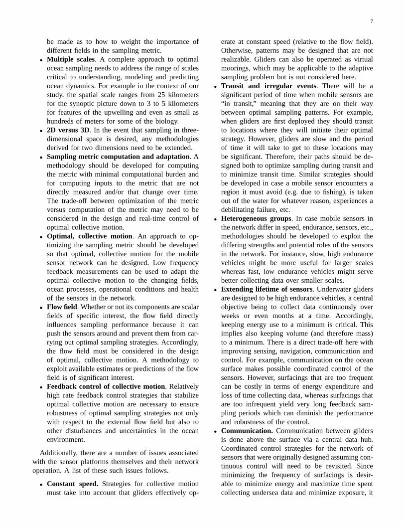
• Constant speed.Strategies for collective motionmust take into account that gliders effectively op-

erate at constant speed (relative to the flow field).Otherwise, patterns may be designed that are notrealizable. Gliders can also be operated as virtualmoorings, which may be applicable to the adaptivesampling problem but is not considered here.

• Transit and irregular events. There will be asignificant period of time when mobile sensors are“in transit,” meaning that they are on their waybetween optimal sampling patterns. For example,when gliders are first deployed they should transitto locations where they will initiate their optimalstrategy. However, gliders are slow and the periodof time it will take to get to these locations maybe significant. Therefore, their paths should be de-signed both to optimize sampling during transit andto minimize transit time. Similar strategies shouldbe developed in case a mobile sensor encounters aregion it must avoid (e.g. due to fishing), is takenout of the water for whatever reason, experiences adebilitating failure, etc.

• Heterogeneous groups. In case mobile sensors inthe network differ in speed, endurance, sensors, etc.,methodologies should be developed to exploit thediffering strengths and potential roles of the sensorsin the network. For instance, slow, high endurancevehicles might be more useful for larger scaleswhereas fast, low endurance vehicles might servebetter collecting data over smaller scales.

• Extending lifetime of sensors. Underwater glidersare designed to be high endurance vehicles, a centralobjective being to collect data continuously overweeks or even months at a time. Accordingly,keeping energy use to a minimum is critical. Thisimplies also keeping volume (and therefore mass)to a minimum. There is a direct trade-off here withimproving sensing, navigation, communication andcontrol. For example, communication on the oceansurface makes possible coordinated control of thesensors. However, surfacings that are too frequentcan be costly in terms of energy expenditure andloss of time collecting data, whereas surfacings thatare too infrequent yield very long feedback sam-pling periods which can diminish the performanceand robustness of the control.

• Communication. Communication between glidersis done above the surface via a central data hub.Coordinated control strategies for the network ofsensors that were originally designed assuming con-tinuous control will need to be revisited. Sinceminimizing the frequency of surfacings is desir-able to minimize energy and maximize time spentcollecting undersea data and minimize exposure, it

8

is of interest to determine the maximum tolerablefeedback sampling period that does not degradeoverall sampling performance as a function of themagnitude of disturbances such as flow.

• Asynchronicity. Strategies will need to accommo-date asynchronicity in time of surfacing and com-munication. Because the gliders will not surfaceat the same time, information communicated to aglider about any of the other gliders will necessarilybe old.

• Latencies. It may not always be possible to closethe feedback loop on the surface. For example, inthe sea trials of 2003, described in SectionIII-B, data retrieved from a glider at its surfacingcould not be used in the waypoint update to theglider at that same surfacing. Instead the data wasused to compute new instructions communicatedto the glider at the next surfacing. This introducessignificant delays that need to be accommodated.

• Computing. While low-level control is computedon board the gliders, coordinated control of thenetwork is computed on the central shore computerwhere inter-glider communication occurs. Possibili-ties for further exploiting on-board computation andlocal measurements should be investigated.

B. Problem Definition

In this paper we address sampling a single time-and space-varying scalar field, like temperature, usingmobile platforms like gliders. Emphasis is on how tooperate such vehicles, either singly or in coordinatedfleets, to provide the most information about this field.Since the main operational control is over course andspeed, we focus on mapping a single 2D horizontalfield. Ultimately the data would be used to describethe 3D field either directly by analysis of 3D dataor by assimilating data into high-resolution dynamicalocean models [32], [33], [34]. However, because oceanscales are similar through the upper water column andhorizontal position is the main control variable, the 2Dproblem suffices.

To measure how well a given sampling array describesthe variable of interest, we adopt a simple metric basedon objective analysis(linear statistical estimation basedon specified field statistics). This metric (defined inSectionV-A) specifies the statistical uncertainty of themodel as a function of where and when the data is taken.Since reduced uncertainty implies better measurementcoverage, we also refer to this as acoverage metric. Inongoing work [2], [35], [36], [37], information that canbe inferred from a dynamical model is included into themetric used to control vehicles.

We frame the optimal collective motion problem anddefine our approach to design of a (near) optimal mobilesensor network in SectionV. By nearoptimal solutions,we mean that we optimize over a parameterized family ofstructured solutions. For example, we consider a familyof closed curves parameterized by number, location,dimension and shape as well as the relative phases of thevehicles moving around these curves. This parameteri-zation is discussed in SectionV-D. The relative phasesprovide a low-dimensional parameterization of relativeposition of the vehicles and they make a connectionbetween the optimized trajectories and the coupled phaseoscillator models that we use in our coordinated controllaw.

We pay particular attention to gliders moving aroundellipses for several reasons. First, the various periodictrajectories appropriate for oceanographic sampling (e.g.,moving back and forth on a line or around a trapezoid asshown in Figures2 and3 from the 2003 AOSN field ex-periment) can be reasonably approximated with ellipsesby tuning the eccentricity. Second, ellipses are minimallyparameterized, smooth shapes for which we have devel-oped a control theoretic framework. In ongoing worknot presented here, we have generalized our controlframework to a class of curves known assuperellipses,which includes circles, ellipses and rounded rectangles.By considering superellipses and optimizing over theparameters that define them, we aim to go beyondthe hand-crafted trajectories of previous experience, toautomate the design, adaptation and control of sensorpatterns that yield maximally information rich data sets.

In the case of gliders moving with constant speedaround circles, the difference in heading for any pair ofgliders can be interpreted as the relative phase of that pairof gliders. For example, if for a pair of gliders movingaround the same circle, the difference in heading is 180degrees, then the relative phase is 180 degrees and thegliders are always at antipodal points on the circle. Forellipses, the relative phase is not necessarily equivalentto the relative heading and so an alternate phase variablebased on arc length along the desired curve can be used.

In SectionVI we present feedback control laws thatstabilize these kinds of collective motions for glidersmoving at constant (unit) speed on the plane. We focuson the case that there may be multiple ellipses andmultiple vehicles per ellipse. The objective is to ensurethat gliders move around their (optimally located, ori-ented and sized) ellipses with optimal relative phases.In SectionVII we compute and study optimal solutionsand we discuss robustness of the solutions with respectto the coverage metric. We also investigate the influenceof the flow field on the design and control of optimal

9

sampling trajectories.In this paper we assume a homogeneous group of

mobile sensors. We do not address the issue of transit andirregular events; preliminary results on minimal time andminimal energy glider paths computed using forecasts ofocean flow fields are presented in [38]. We also do notaddress the problems in communication, asynchronicity,latency and computing described above. In [30], [13] itis discussed how these issues were handled in AOSN2003. In [39] a control law is presented that exploresextended sensing, computing and control onboard aglider. In this paper we let each sensor compute its owncontrol law locally and we assume continuous feedbackcontrol with continuous communication without delay orasynchronicity. Because communication is not limitedto neighboring gliders in the operational scenario, weassume an all-to-all interconnection topology.

A number of the issues listed in SectionIV-A remainimportant open problems and are the subject of ongoingwork.

V. SAMPLING METRIC AND OPTIMALITY

A. Sampling Metric

In this section, we derive a metric to quantify how wellan array of gliders samples a given region. Recall thatan objective is to assimilate the data in an ocean model.Therefore, the metric should reflect how a particulardata set reduces the error in the model. This notion isnecessarily dependent on the specific model or assimi-lation scheme used. During AOSN 2003, the data wasassimilated in several high resolution ocean models [32],[33], [34] and the performance of the sampling array wassimilar for each. Since reliable nowcasts and forecastsof the ocean require concurrent ocean models mutuallyvalidating their results and the data requirements of thesemodels are similar, it is natural to derive the performancemetric on a simpler, more general assimilation scheme.This approach also has the advantage of avoiding thecomplexity and computational effort required to studyspecific high resolution models [40], [41]. To computeour metric we need only a background covariancefunction to describe the field and the locations andtimes corresponding to where and when the data wascollected; the measurements and forecast of the field arenot needed.

We consider a simple data assimilation scheme calledobjective analysis2 [42], [43]. In this framework, the

2Objective analysis is also commonly referred to as optimal inter-polation. It was originally developed by Eliassen et al [14] in 1954and independently reproduced and popularized by Gandin [15] in1963.

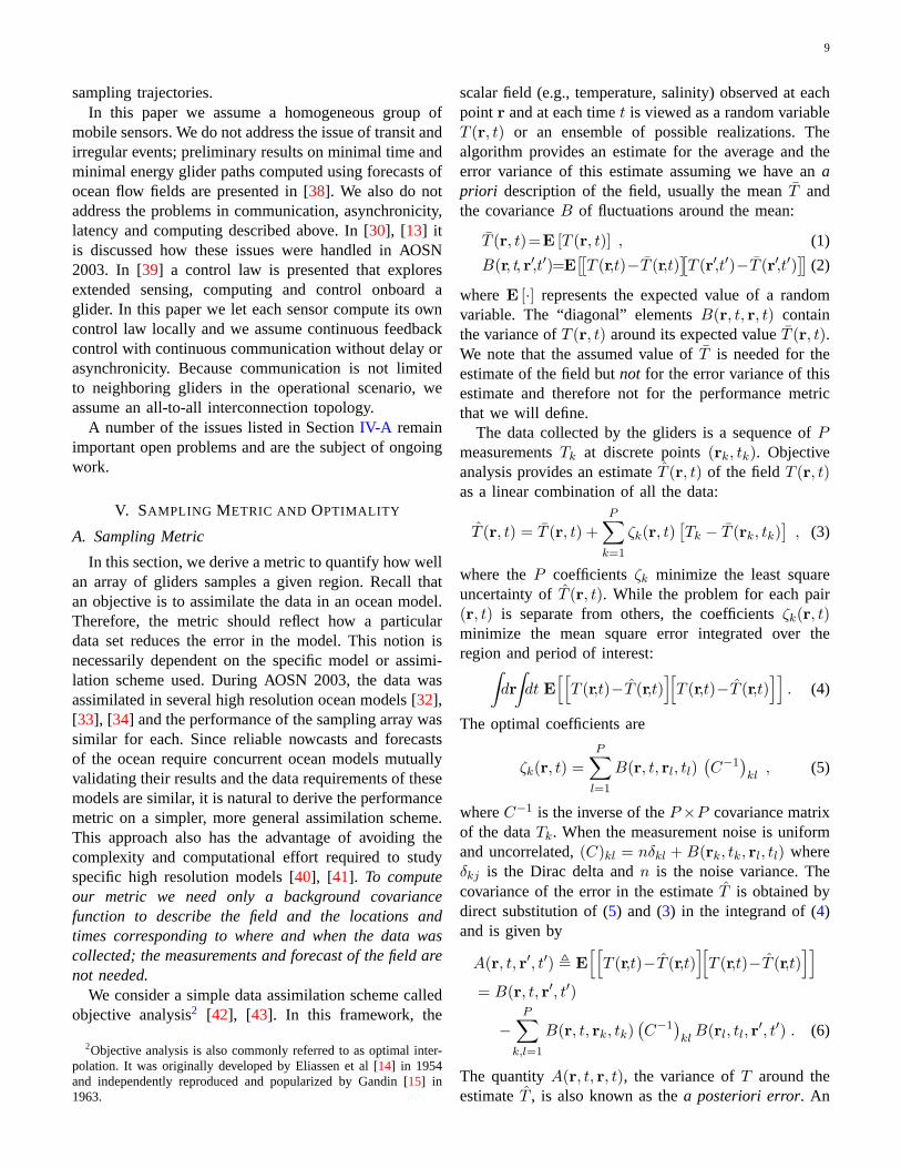
scalar field (e.g., temperature, salinity) observed at eachpoint r and at each timet is viewed as a random variableT (r, t) or an ensemble of possible realizations. Thealgorithm provides an estimate for the average and theerror variance of this estimate assuming we have anapriori description of the field, usually the meanT andthe covarianceB of fluctuations around the mean:

T (r, t)=E [T (r, t)] , (1)

B(r, t, r′,t′)=E[[T (r,t)−T (r,t)

][T (r′,t′)−T (r′,t′)

]](2)

whereE [·] represents the expected value of a randomvariable. The “diagonal” elementsB(r, t, r, t) containthe variance ofT (r, t) around its expected valueT (r, t).We note that the assumed value ofT is needed for theestimate of the field butnot for the error variance of thisestimate and therefore not for the performance metricthat we will define.

The data collected by the gliders is a sequence ofPmeasurementsTk at discrete points(rk, tk). Objectiveanalysis provides an estimateT (r, t) of the fieldT (r, t)as a linear combination of all the data:

T (r, t) = T (r, t) +P∑k=1

ζk(r, t)[Tk − T (rk, tk)

], (3)

where theP coefficientsζk minimize the least squareuncertainty ofT (r, t). While the problem for each pair(r, t) is separate from others, the coefficientsζk(r, t)minimize the mean square error integrated over theregion and period of interest:∫

dr∫dt E

[[T (r,t)−T (r,t)

][T (r,t)−T (r,t)

]]. (4)

The optimal coefficients are

ζk(r, t) =P∑l=1

B(r, t, rl, tl)(C−1

)kl, (5)

whereC−1 is the inverse of theP×P covariance matrixof the dataTk. When the measurement noise is uniformand uncorrelated,(C)kl = nδkl + B(rk, tk, rl, tl) whereδkj is the Dirac delta andn is the noise variance. Thecovariance of the error in the estimateT is obtained bydirect substitution of (5) and (3) in the integrand of (4)and is given by

A(r, t, r′, t′) , E[[T (r,t)−T (r,t)

][T (r,t)−T (r,t)

]]= B(r, t, r′, t′)

−P∑

k,l=1

B(r, t, rk, tk)(C−1

)klB(rl, tl, r′, t′) . (6)

The quantityA(r, t, r, t), the variance ofT around theestimateT , is also known as thea posteriori error. An

10

extensive analysis of the assimilation scheme, equationsand generalizations (e.g., multivariate, discrete, non-stationary systems) can be found in [42], [43].

Because estimation errors of a hypothetical samplingarray are determined by the statistics of the field noise,A(r, t, r, t) can be used as a quantitative measure of theimpact of a sequence of measurements on knowledge ofthe field and allowa priori design of effective samplingarrays [16]. In this paper, the integral ofA(r, t, r, t) overthe domain,

φ ,∫dr

∫dt A(r, t, r, t) , (7)

equivalent to (4) evaluated at the optimalT , is electedas the sampling performance metricto compare andoptimize sampling strategies. Substitution of (6) in (7)gives

φ =∫dr

∫dt (B(r, t, r, t)

−P∑

k,l=1

B(r,t,rk,tk)(C−1

)klB(rl,tl,r,t)

). (8)

Note that this metric depends only on the covariancefunctionB and the measurement locations and times,rkandtk.

B. Ocean Statistics

The coverage metric defined in (8) requires speci-fication of the term,B(r, t, r′, t′), an estimate of thebackground statistics. It represents the estimated statis-tics of the oceanbefore data assimilation. The diag-onal elementsB(r, t, r, t) describe our confidence inthe initial state. The non-diagonal elements representthe covariance between points at different locations andtimes. They are closely related to the correlation lengthand the correlation time in the domain [16].

The metric in (8) has a broad range of applicationand can be used with any positive-definite covariancefunction B(r, t, r′, t′). For the purpose of illustratingthe use of the metric, we assume that the backgroundcovariance is given by

B(r, t, r′, t′) , σ0 e−‖r−r′‖2

σ2 −|t−t′|2τ2 . (9)

The parametersσ and τ are thea priori spatial andtemperature decorrelation scales; because (9) fixes thestructure of the unknown termB, σ andτ can be viewedas inputs to the objective analysis algorithm. In thispaper we useσ = 25 km and τ = 2.5 days; thesevalues were determined empirically using glider datafrom Monterey Bay during AOSN 2003 [28]. Notice

Num

bero

fmea

sure

men

ts/d

ay

0

300

600

900

Time (days since January 1st 2003)200 210 220 230 240 2500

0.025

0.05

0.075

0.1

0.125

0.15

0.175

0.2

PSfrag replacements

I(t

)

Fig. 6. Sampling metric (solid curve) in units of entropic information(see (10)) and number of profiles (shadowed area) for AOSN 2003.Each cross correspond to a panel of Fig.5. On August 10th (day223), the number of profiles is still high but the metric indicatesrelatively poor coverage. The second panel of Fig.5 explains thisloss of performance by a poor distribution of the gliders in the bayon that day.

that the scaling factorσ0 has no effect on the samplingpaths, provided that the measurement noisen is scaledby the same factor. This fact is discussed and exploitedin SectionVII .

Figure 5 shows a map of thea posteriori errorA(r, t, r, t) at different times during AOSN 2003 wherethe background covariance is modelled as Gaussian as in(9). The data used correspond to the Spray gliders [22],[28] and the Slocum gliders [13], [28] that patrolled inand around Monterey Bay during the summer of 2003(as plotted in Figures2 and3).

The metricφ, as defined in (8), represents the per-formance for the entire experiment. To visualize theperformance as a function of time, we omit the integralover time in (8) and define

I(t) = − log(

1σ0A

∫drB(r, t, r, t)

), (10)

whereA is the area of the spatial domain. The functionI(t) is plotted on Fig.6 and represents the entropicinformation [44] during the AOSN 2003 experiment.

C. Optimal and Near-Optimal Collectives

In the context of ocean sampling, not only can (8) beused to quantify the performance of a particular arrayor formation, but it also provides a means to search foroptimal sampling strategies. The glider array is viewedas a set ofN trajectoriesrk(t) satisfying the constraint

rk(t) = v, k = 1, . . . , N , (11)

11

Longitude (degrees)

Latit

ude

(deg

rees

)

-123.5 -123.0 -122.5 -122.0

36.0

36.2

36.4

36.6

36.8

37.0

37.2

37.4

Aug 01, 2003 06:00:00

Longitude (degrees)

Latit

ude

(deg

rees

)

-123.5 -123.0 -122.5 -122.0

36.0

36.2

36.4

36.6

36.8

37.0

37.2

37.4

Aug 05, 2003 08:00:00

Longitude (degrees)

Latit

ude

(deg

rees

)

-123.5 -123.0 -122.5 -122.0

36.0

36.2

36.4

36.6

36.8

37.0

37.2

37.4

Aug 10, 2003 18:00:00

Longitude (degrees)

Latit

ude

(deg

rees

)

-123.5 -123.0 -122.5 -122.0

36.0

36.2

36.4

36.6

36.8

37.0

37.2

37.4

Aug 14, 2003 22:00:00

Fig. 5. Error map at different times during the AOSN 2003 experiment. Blue represents small error (good coverage) and red and whiterepresents high error (poor coverage). For each panel, black dots indicates the reported position of the vehicles at the given time. The whitedots represent their positions during the last 12 hours. The magenta line encloses all the points where the error has been reduced from itsinitial state by at least 85%. The sampling metric is shown on Fig6. Notice that all the gliders are clustered near the coast on August 10thexplaining the drop in coverage performance visible on Fig.6.

where v is velocity relative to the flow and speed‖v‖ = v is fixed. Each glider generates a sequence ofmeasurements(rlk, tl) = (rk(l∆t), l∆t), where∆t is thesampling period, i.e. the time between profiles. The setof all measurements at a particular depth gathered bytheN gliders can be substituted in (8) to determine theperformance of the array that we write asφ(~r), where~r = (r1, . . . , rN )T . A set of optimal trajectories for thesegliders is a set ofN curves satisfying (11) and such thatφ(~r) is minimum.

Such optimal trajectories are usually complicated andunstructured. In addition, their computation requires aminimization in a large functional space, which may notalways be desirable for real-time applications. In thiswork, rather than optimizing individual trajectories, weoptimize collective patterns parameterized by a restrictednumber of parameters. For example, SectionsVI andVII

focus on arrays of vehicles moving around ellipses.For such trajectories the parameters are the numberof ellipses and the number of vehicles per ellipse, theposition, size and eccentricity of each ellipse as wellas the relative position of each pair of vehicles as theymove around their ellipses (formulated below as relativephases). Clearly, the computation of the minimum inparameterized families is a much more tractable prob-lem. However, the interest in optimizing the samplingperformance over parameterized collectives rather thanover individual trajectories extends beyond the numericalconvenience. Parameterized collectives are essential toachieve the following:

• Closed-loop control.For each proposed collective,a feedback control is designed that makes it anexponential attractor of the closed-loop dynamics.Feedback control of the collective motion provides

12

robustness for the relative motion of the vehicles incontrast to a decentralized tracking control of eachvehicle along its individual reference trajectory.

• Robustness. The robustness of an optimal collec-tive can be studied in terms of the derivatives of themetric with respect to the parameters of the family(see SectionVI andVII ). Small second derivativesindicate flat minima and solutions that are morerobust to perturbations such as uncertainty in GPSmeasurements, deviations due to the flow field orcommunication problems.

• Interpretation of the data. By restricting thechoice of collectives to specific geometries, thedata collected along these paths can more easily beinterpreted in terms of oceanographic sections [45].

In SectionVI , we present the development of coor-dinated control for gliders on circles and on ellipses. InSectionVII , we investigate a parameterized family ofelliptical collectives in more detail and determine theoptimal collective within this parameterized family.

D. Parameterization of collectives

Parameterized families of collectives over closedcurves involving the least number of parameters arecircles. If we specialize to circles, the optimal parametersto be computed are the number of circles, the number ofgliders per circle, the origin and radius of each circle andthe relative positions of the gliders on their respective cir-cles. The relative position of two gliders moving aroundthe same circle can be represented by the difference intheir headings; this difference is fixed since the glidersmove at constant speed. The difference in the headingsis equal to the relative phase of the gliders around thecircle. To see this suppose the gliders move at unit speedaround a single circle of radiusρ0 = |ω0|−1 and centeredat the origin. The position of thekth glider at timet isrk(t) = ρ0(cos(ω0t+γk), sin(ω0t+γk)), whereγk is thephase of thekth glider. The derivative ofrk with respectto time is rk = sgn(ω0)(sin(ω0t + γk), cos(ω0t + γk)).The velocity of the glider can also be expressed asrk = (cos θk, sin θk) where θk is the glider’s headingangle. By equating these two expressions forrk we getω0t+ γk + sgn(ω0)π/2 = θk. Thus, the relative headingof two vehicles is equal to their relative phase, i.e.,θj − θk = γj − γk. In the top left panel of Figure7,two vehicles move around circles withγ2 − γ1 = 0. Inthe top right panel,γ2 − γ1 = π.

Suppose now that two gliders move at unit speed abouttwo different circles, each with radiusρ0 and the samedirection of rotation but with non-coincident centers.In this case the relative heading (and therefore relative

(a)

!1 = !2

"1 = "2

(b)

!1

!2 "1"2

(c)

!0!0

d0

d0 ! 2!0

d0 + 2!0 (d)

L = 4

Fig. 7. Cartoons of vehicles moving around closed curves withprescribed relative phases; a) Two vehicles with relative phase equalto zero move around a circle; b) Two vehicles with relative phaseequal toπ move around a circle; c) Two vehicles with relative phaseequal toπ and each vehicle moving around a different circle; d) Aclosed curve with rotational order of symmetryL = 4. Four vehiclesmove around it with fixed relative phase.

phase) of the two gliders remains constant and therelative position of the gliders is periodic. The periodicfunction can easily be described by the relative phase andrelative position of the circle origins. Let the distancebetween the circle origins bed0. Then, if the relativephase is zero, the gliders are synchronized and theirrelative distance remains constant and equal tod0. Ifthe relative phase isπ then the relative distance of thevehicles varies from its minimum atd0 − 2ρ0 to itsmaximum atd0 + 2ρ0. This is illustrated in the bottomleft panel of Figure7.

Because relative phase is constant for vehicles movingat constant speed around circles of the same radius anddirection of rotation, we parameterize relative positionof a pair of gliders by their relative phase. This makesthe stabilizing control problem one of driving vehiclesto circles of given radius with prescribed, fixed, relativephases (equivalently, relative headings). For example,supposeN gliders are to move around the same circle.An example of an optimal solution in a homogeneousfield is one in which the gliders are uniformly distributedaround the circle (called thesplay state formation).This is equivalent to phase locking with relative phasebetween neighboring gliders equal to2π/N , which westudy in the next section.

Relative phase can be useful as a prescription ofrelative position even for closed curves of more generalshape. The choices of relative phase that can be keptconstant for constant speed vehicles moving around agiven shape depend on therotational order of symmetryof the shape. The rotational order of symmetry of ashape is equal toL ∈ N0 if the shape looks unchanged

13

after it is rotated about its center by angle2π/L. Forexample, a hexagon has rotational symmetry of ordersix, a square has symmetry of order four, a rectangleand an ellipse have symmetry of order two. A shapewith rotational order of symmetry equal to one has norotational symmetry.

Consider a shape with rotational order of symmetryequal toL. If we choose the relative phase for a pairof gliders moving at constant speed around the shape tobe an integer multiple of2π/L, the relative phase willremain constant. An example forL = 4 is shown inFigure7. In the case of circles, as discussed above, anyrelative phase can be selected. In the case of ellipses,only two choices of relative phase can be selected; theseare either relative phase equal to zero or equal toπ,when the gliders are synchronized or anti-synchronized,respectively, as they move around a single ellipse or upto N identical ellipses with non-coincident centers.

In SectionVI we describe steering control laws forstabilization of gliders to circles and ellipses with phaselocking.

VI. COORDINATED CONTROL

This section describes feedback control laws that sta-bilize collective motion of a planar model of autonomousvehicles moving at constant speed. Following SectionV,we consider vehicles moving around closed curves withgiven, fixed relative phases. As described in SectionV-D,relative phases determine, in part, the relative positionsof the vehicles. In the case of collective motion aroundcircles of equal radius and direction of rotation, therelative phase is identical to relative heading and is alsoconstant. For more general shapes, prescribed relativephases are chosen as an integer multiple of2π/L whereL is the rotational order of symmetry of the shape. Forexample, in the case of coordinated motion of glidersaround ellipses,L = 2 and we design stabilizing con-trollers that fix relative phases to 0 orπ. This restrictioncan be relaxed using an alternate definition of relativephase based on arc length along the desired curve; thisis the subject of ongoing work and will be presented ina forthcoming paper.

Each glider is modeled as a point mass with unitmass, unit speed and steering control. We first provide afeedback control law that stabilizes circular motion of thegroup of vehicles about its center of mass. This controllaw depends on the relative position of the vehicles.Next, we address the problem of stabilizing the relativephases of the circling vehicles. An additional controlterm, depending only on the relative headings of thevehicles, stabilizes symmetric patterns of the vehiclesin the circular formation.

As long as the feedback control is a function onlyof the relative positions and headings of the vehicles,the system dynamics are invariant to rigid rotation andtranslation of the whole vehicle group in the plane. Thiscorresponds to the symmetry group,SE(2) = SO(2)⊗R2 ≡ S1⊗R2, where⊗ is the semi-direct product. HereSO(2) = {X ∈ R2×2 | XTX = I,det(X) = 1} is thespecial orthogonal group in the plane and describes thespace of all 2D rotations.SO(2) is equivalent toS1, theone-dimensional sphere or circle, since there is a one-to-one relationship between rotations in the plane andangles in[0, 2π). SE(2) is the special Euclidean groupin the plane and describes the space of all possible rigidrotations and translations in the plane. We show howbreaking this symmetry, i.e., by introducing a controlterm that depends on the position and/or orientation ofthe group as a whole, can lead to useful variations oncircular formations. First, we introduce a fixed beacon tobreak theR2 symmetry. Second, we introduce a refer-ence heading which breaks theS1 symmetry. In addition,we introduce interconnection topologies for the spacingand orientation coupling that stabilize collective motionof coordinated subgroups of vehicles. This includes thecase in which there are multiple circles with a differentsubgroup of vehicles moving around each circle.

Finally, we describe a control law to stabilize collec-tive motion on more general shapes. More specifically,we stabilize a single vehicle on an elliptical trajectoryabout a fixed beacon. Additionally, we couple vehicleson separate ellipses using their relative headings in orderto synchronize the vehicle phases about each ellipse.

A. Circular Control

The vehicle model that we study is composed ofNidentical point-mass vehicles subject to planar steeringcontrol. The vehicle model is

rk = veiθk

θk = uk, k = 1, . . . N (12)

whererk = xk + iyk ∈ C ≡ R2 and θk ∈ S1 are theposition and heading of each vehicle,v is the vehiclespeed relative to the flow, anduk is the steering controlinput to the kth vehicle. In this section, we assumeunit vehicle speed, i.e.v = 1, and ignore the flow. InSectionV, the positionrk of thekth vehicle was a vectorin R2.

In this section, we exploit the isometry betweenR2

andC and we viewrk as an element of thereal3 vector

3By real vector space, we mean a vector space for which the fieldof scalars isR. Complex vector spaces are defined with complexscalars. For example,CN is both a real and a complex vector space.In this paper, we considerCN as a real vector space only.

14

spaceC. The real vector spacesC andCN give us moreflexibility in choosing an inner product4. We define theinner product by

〈z1, z2〉 = Re{z>1 z2} , (13)

where zT1 represents the conjugate transpose ofz1 andRe {·} is the real part of a complex number. We viewz1 and z2 as the elements of the real vector spaceCN

(i.e., isomorphic toR2N ), for which (13) is a valid innerproduct.

For the sake of brevity, we often stack identical vari-ables for each vehicle in a common vector. For example,~θ = (θ1, . . . θN )T ∈ TN contains all the headings and~r = (r1, . . . rN )T ∈ CN contains all the positions.

To help understand the model (12), consider thefollowing two examples of constant control input. Foruk = ω0 6= 0, the vehicles travel on fixed circles ofradius ρ0 = |ω0|−1. The sense of rotation is given bythe sign ofω0. For uk = ω0 = 0, each vehicle follows astraight trajectory in the direction of the initial heading.

Due to the unit speed and unit mass assumptionswe can relate the coherence of vehicle headings to themotion of the group. Let the center of mass of thegroup beR = 1

N

∑Nj=1 rj . Also, let theorder parameter

p~θ ∈ C, denote the centroid of the vehicle headings onthe unit circle in the complex plane. The order parameteris equivalent to the velocity of the center of mass of thegroup, i.e.

p~θ ,1N

N∑k=1

eiθk =1N

N∑k=1

rk = R.

Notice that we have0 ≤∣∣p~θ∣∣ ≤ 1. We define a potential

functionU1 by

U1(~θ) =N

2|p~θ|

2. (14)

The gradient ofU1 is given by

∂U1

∂θk=

⟨ieiθk ,p~θ

⟩, k = 1, . . . , N. (15)

Certain distinguished motions of the group correspondto critical points ofU1. For instance,U1(~θ) is maximumfor parallel motion of the group (∀ k : θk = θ0)and minimum when the center of mass is fixed (p~θ =R = 0). We refer to solutions for whichp~θ = R = 0asbalancedsolutions since the headings are distributedaround the unit circle so that the center of mass of thegroup is fixed. Letting~1 = (1, · · · , 1) ∈ RN , we use

4〈z1, z2〉 = Re˘z>1 z2

¯is not an inner product for the complex

vector spacesC because it violates sesquilinearity. However, it is avalid inner product for the real vector spacesC andCN .

(15) to observe that⟨∇U1,~1

⟩=

⟨ip~θ,p~θ

⟩= 0; this

corresponds to theS1 rotational symmetry of the systemsince U1 is invariant to rigid rotation of the vehicleheadings.

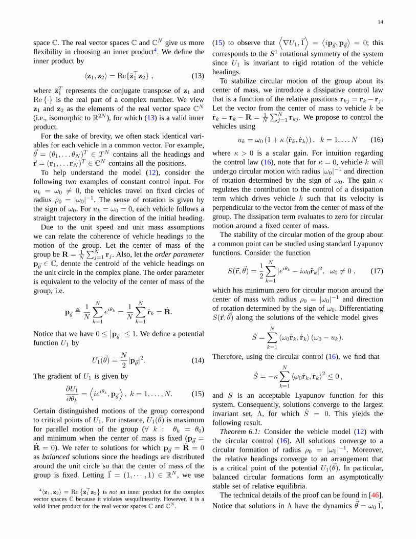
To stabilize circular motion of the group about itscenter of mass, we introduce a dissipative control lawthat is a function of the relative positionsrkj = rk− rj .Let the vector from the center of mass to vehiclek berk = rk −R = 1

N

∑Nj=1 rkj . We propose to control the

vehicles using

uk = ω0 (1 + κ 〈rk, rk〉) , k = 1, . . . N (16)

where κ > 0 is a scalar gain. For intuition regardingthe control law (16), note that forκ = 0, vehiclek willundergo circular motion with radius|ω0|−1 and directionof rotation determined by the sign ofω0. The gainκregulates the contribution to the control of a dissipationterm which drives vehiclek such that its velocity isperpendicular to the vector from the center of mass of thegroup. The dissipation term evaluates to zero for circularmotion around a fixed center of mass.

The stability of the circular motion of the group abouta common point can be studied using standard Lyapunovfunctions. Consider the function

S(~r, ~θ) =12

N∑k=1

|eiθk − iω0rk|2, ω0 6= 0 , (17)

which has minimum zero for circular motion around thecenter of mass with radiusρ0 = |ω0|−1 and directionof rotation determined by the sign ofω0. DifferentiatingS(~r, ~θ) along the solutions of the vehicle model gives

S =N∑k=1

〈ω0rk, rk〉 (ω0 − uk).

Therefore, using the circular control (16), we find that

S = −κN∑k=1

〈ω0rk, rk〉2 ≤ 0 ,

and S is an acceptable Lyapunov function for thissystem. Consequently, solutions converge to the largestinvariant set,Λ, for which S = 0. This yields thefollowing result.

Theorem 6.1:Consider the vehicle model (12) withthe circular control (16). All solutions converge to acircular formation of radiusρ0 = |ω0|−1. Moreover,the relative headings converge to an arrangement thatis a critical point of the potentialU1(~θ). In particular,balanced circular formations form an asymptoticallystable set of relative equilibria.

The technical details of the proof can be found in [46].

Notice that solutions inΛ have the dynamics~θ = ω0~1,

15

i.e. vehicles follow circles of radius|ω0|−1. The setof balanced circular solutions for which all circles arecoincident corresponds to the minimum of the potentialS(~r, ~θ). Simulations suggest that this set of equilibriahas almost global convergence.

B. Control of Relative Headings

If, in addition to the relative positions, we feed backthe relative headings of the vehicles, we can stabilizeparticular phase-locked patterns or arrangements of thevehicles in their circular formation. Let the potentialU(~θ) satisfy

⟨∇U,~1

⟩= 0 so that it is invariant to

rigid rotation of all the vehicle headings. We combinethe circular control (16) with a gradient control term asfollows:

uk = ω0 (1 + κ 〈rk, rk)〉 −∂U

∂θk. (18)

The circular motion of the group in a phase-lockedheading arrangement is a critical point ofU(θ). Thestability of the motion can be proved by showing theexistence of a Lyapunov function. For instance take,

V (~r, ~θ) = κS(~r, ~θ) + U(~θ), (19)

whereS(~r, ~θ) is defined in (17). The time derivative ofV (~r, ~θ) along the solutions of the vehicle dynamics isgiven by

V =N∑k=1

(κ 〈ω0rk, rk〉 −

∂U

∂θk

)(ω0 − uk). (20)

Substitution of the composite control (18) in (20) gives

V = −N∑k=1

(κ 〈ω0rk, rk〉 −

∂U

∂θk

)2

≤ 0.

Therefore, solutions converge to the largest invariant set,Λ, for which V = 0. A detailed proof can be foundin [46] and yields the following theorem

Theorem 6.2:Consider the vehicle model (12) and asmooth heading potentialU(θ) that satisfies

⟨∇U,~1

⟩=

0. The control law (18) enforces convergence of allsolutions to a circular formation of radiusρ0 = |ω0|−1.Moreover, the relative headings converge to an arrange-ment that is a critical point of the potentialκU1 + U .In particular, every minimum ofU for which U1 = 0defines an asymptotically stable set of relative equilibria.

This result enables us to stabilize symmetric pat-terns of the vehicles in circular formations. Symmetric(M,N)-patterns of vehicles are characterized by2 ≤M ≤ N heading clusters separated by a multiple of2πM . Figure8 depicts the six possible different symmetric

Fig. 8. The six possible different symmetric patterns forN =12 corresponding toM = 1, 2, 3, 4, 6 and 12. The top left is thesynchronized state and the bottom right is thesplay state. The numberof collocated headings is illustrated by the width of the black annulusdenoting each phase cluster.

phase patterns forN = 12; it is not meant to implythat the vehicles are collocated, rather that their velocityphasors may be. There is a one-to-one correspondencebetween these symmetric patterns and global minima ofspecifically designed potentials [46]. In order to definethese potentials, we extend the notion of the order pa-rameter of vehicle headings to include higher harmonics,i.e.

pm~θ

=1mN

N∑k=1

eimθk .

The objective is to consider potentials of the form

Um(~θ) =N

2|pm~θ|2,

which satisfy⟨∇Um,~1

⟩= 0. These potentials are used

to prove the following [46]:Lemma 6.1:Let 1 ≤M ≤ N be a divisor ofN . Then

~θ ∈ TN is an(M,N)-pattern if and only if it is a globalminimum of the potential

UM,N =M∑m=1

KmUm

whereKm are arbitrary coefficients satisfyingKm > 0,m = 1, . . . ,M − 1 andKM < 0.

Theorem6.2 together with Proposition6.1 yield aprescription for stabilizing symmetric patterns. Of par-ticular interest for mobile sensor networks is stabilizingthe circular formation in which the vehicles are evenlyspaced, i.e. the(N,N)-pattern orsplay stateformation[47]. This formation is characterized byp

m~θ= 0 for

m = 1, . . . N − 1 and |pN~θ| = 1

N . Since pm~θ

= 0imposes two constraints on the relative phases for eachm, we need only specify the first

⌊N2

⌋harmonics, where

16

−30 −20 −10 0 10 20

−20

−10

0

10

x

y

Fig. 9. A numerical simulation of the splay state formation startingfrom random initial conditions using the control (22) with N = 12,ω0 = 0.1, κ = ω0 andK = ω2

0 . Each vehicle and its velocity isillustrated by a black circle and an arrow. Note that the center of massof the group, illustrated by a crossed circle, is fixed at steady-state.

⌊N2

⌋is the largest integer less than or equal toN

2 [46].Consequently, we define the splay state potential to be

UN,N = K

bN

2 c∑m=1

Um, K > 0. (21)

The splay state formation control law has the form (18)with U(~θ) given by (21) and can be written

uk = ω0(1+κ 〈rk, rk〉)+K

N

N∑j=1

bN/2c∑m=1

sinmθkjm

. (22)

A simulation of the splay state formation forN = 12vehicles is shown in Figure9. Twelve vehicles start fromrandom initial conditions and the controller (22) enforcesconvergence to a circular orbit with uniform spacing (i.e.,the phase difference between adjacent vehicles is2π

12 ).

C. Planar Symmetry Breaking

The feedback control laws in sectionsVI-A andVI-Brequire only the relative positions and headings of thevehicles and, consequently, they are invariant to rigidtranslation and rotation in the plane. This corresponds tothe symmetry group,SE(2) ≡ S1 ⊗R2. In this section,we introduce variations of these control laws which breakthe translation and rotation symmetries. First, we breakthe R2 translation symmetry by stabilizing the circularformation about a fixed beacon. Secondly, we break theS1 rotational symmetry by coupling the vehicles to aheading reference.

The position of the fixed beacon is referred to asR0 ∈ C. The relative position from the beacon is definedas rk = rk − R0. A formal proof uses the Lyapunov

function S(~r, ~θ) defined in (17) with the new definitionof rk. Furthermore, Theorem6.2 continues to hold forcircular motion about the fixed beacon [46]. That is, thecontrol (18) can be used to stabilize circular motion tothe set of heading arrangements that are critical pointsof the potentialU(~θ), where

⟨∇U,~1

⟩= 0. Clearly, this

applies to the splay state potential (21).Next, we introduce a heading referenceθ0 whereθ0 =

ω0. Let uk, k = 1, . . . , N − 1 be given by (18) whereU(~θ) is a potential that satisfies

⟨∇U,~1

⟩= 0. TheN th

vehicle is coupled to the heading reference using

uN = ω0(1 + κ(rk, rk))−∂U

∂θk+ d sin(θ0−θN ), (23)

whered > 0. Critical points ofU(~θ) that satisfyθN = θ0define an asymptotically stable set [46]. To prove thisresult, we use the composite Lyapunov function

W (~r, ~θ) = V (~r, ~θ) + d(1− cos(θ0 − θN ))

whereV (~r, ~θ) is given by (19). The complete analysiscan be found in [46]. The set of circular formations thatminimizesU(~θ) and satisfiesθN = θ0 are the globalminima ofW (~r, ~θ). For ω0 = 0, the control (23) can beused to track piecewise linear trajectories [48].

D. Coordinated Subgroups

In this section, we design control laws to coordinatevehicles in subgroups usingblock all-to-all intercon-nection topologies. Here, the term “block” refers to asubgroup of vehicles and “all-to-all” refers to the inter-connection topology of that subgroup. It is assumed thatthe subgroups are not interconnected unless otherwisestated. In other words, the vehicles can be distributedamong subgroups, in which each subgroup correspondsto vehicles moving on a different circle or ellipse. First,we introduce a block all-to-all interconnection topologyfor the circular control term that depends on the relativepositions. This restriction on the coupling yields stabilityof subgroups of vehicles in separate circular formations.Similarly, block all-to-all coupling applied to the gradientcontrol term that depends on relative headings yieldsheading arrangements within subgroups of vehicles. Weillustrate the use of block all-to-all couplings on a sce-nario of practical interest. The vehicles are divided intothree subgroups that minimize the splay state potentialsuch that each subgroup is in a splay state formation.

We refer to each vehicle subgroup by its block indexb = 1, . . . , B, whereB is the total number of blocks.Let N b be the number of vehicles in blockb. Note thatN b ≥ 2 except in the case of fixed beacons in whichN b ≥ 1.

17

We assume that each vehicle is assigned to one andonly one block, so that

∑Bb=1N

b = N . Also, let F b ={f b1 , . . . , f bNb} be the set of vehicle indices in blockb.The center of mass of blockb is given by

Rb =1N b

Nb∑k=1

rfbk.

Similarly, them-th moment of the heading distributionof block b is

pbm~θ

=1

mN b

Nb∑k=1

eimθfb

k , m = 1, 2, . . . . (24)

Using (24), we can also define block-specific headingpotentials such as

U bm(~θ) =12|pbm~θ|2. (25)

Note that ∂(Ubm)

∂θk= 0 for k /∈ F b and

⟨∇U bm,~1

⟩= 0.

Using this notation, we summarize the followingcorollaries to Theorems6.1and6.2. First, consider blockall-to-all coupling for the circular control term only. Inthis case, the control law (18) with rk = rk − Rb andk ∈ F b enforces convergence of all solutions to circularformations of radiusρ0 = |ω0|−1 in phase arrangementsthat are critical points of the potentialκU b1 + U as inTheorem6.2, whereU(~θ) is a potential that satisfies⟨∇U,~1

⟩= 0. In particular, the circular motion of all the

vehicles in a block have coincident centers. Alternatively,suppose we use block all-to-all coupling only in thegradient control term that depends on relative headings.In this case, the control law is (18), where U(~θ) =∑B

b=1 Ub(~θ) andU b(~θ) is a potential depending only on

the headings in blockb that satisfies⟨∇U b,~1

⟩= 0. This

control enforces convergence of all solutions to circularformations of radiusρ0 = |ω0|−1 in phase arrangementsthat are critical points of the potentialsκU1 + U b.

To demonstrate the use of the control law (18), wepresent the result of a useful case of block all-to-allspacing coupling with fixed beacons. In this example,the phase coupling is both all-to-all and block all-to-allwith

U = U (N,N) +B∑b=1

U b (Nb,Nb) (26)

whereN b = N/B for b = 1, . . . , B and isU b (Nb,Nb) isgiven by (21). This potential is minimized by the phasearrangement in which the entire group, as well as eachblock, are in the splay state of vehicle headings. In otherwords, if all the vehicle heading phasors were plotted onthe same unit circle, then the resulting pattern would bethe splay state forN headings (see Figure (8). Taken

−40 −20 0 20 40 60−40

−20

0

20

40

x

y

Fig. 10. Simulation results forN = 12 andB = 3 starting fromrandom initial conditions with block all-to-all spacing coupling andthree fixed beacons at(R1

0,R20,R

30) = (−30, 0, 30). Phase coupling

is all-to-all and block all-to-all with the potential (26). The simulationparameters areκ = ω0 = 1/10.

separately, the headings phasors for blockb are also inthe splay state forN b headings. Simulation results forN = 12 andB = 3 are shown in Figure10. The twelvevehicles start from random initial positions and organizethemselves in the splay states using (18).

E. Shape Control: Elliptical Beacon Control Law

In this section, we modify the circular control lawand stabilize a single vehicle on an elliptical trajectoryabout a fixed beacon. We use a generalization of thepotentialS(~r, ~θ) in (17) to prove Lyapunov stability ofthis trajectory. Additionally, we couple several vehiclesvia their relative headings as in SectionVI-B in order tosynchronize the vehicle phases on each ellipse.

Let R0 ∈ C and µ0 ∈ S1 represent the center andorientation of an ellipse with the lengths of the semi-major and -minor axes given bya and b. The positionsof the focii areR0 ± c eiµ0 , wherec =

√a2 − b2. Let

d ∈ C andd′ ∈ C be the relative positions of the singlevehicle from each focus, defined by

d , ρ ei(ψ+µ0) = r−R0 − c eiµ0 (27)

d′ , ρ′ ei(ψ′+µ0) = r−R0 + c eiµ0 (28)

and shown in Panel (a) of Figure11.For a single vehicle whose position and heading

are r and θ, respectively, motion along the ellipse ischaracterized by

ρ+ ρ′

2= a (29)

andψ + ψ′

2= θ − µ0 ±

π

2. (30)

18

(a)

d

d!

R0

c

rµ0

r

x

y

(b)

! ! µ0

"

#

#!

x

y

$

Fig. 11. a) The vectorsd andd′ used to identify the position of thevehicle (larger white circles) relative to the focii (solid circles) for anellipse centered atR0 and rotated byµ0. b) Depicts the anglesψ,ψ′, α, andλ used in the control design. Note thatλ = 0 for stableelliptical motion with positive rotation.

Condition (29) requires that the average distance tothe focii remains constant. Condition (30) requires thatthe average angular position measured from both fociimust be separated by±π

2 from the angle made bythe velocity vector and the major axis. Notice that theterm ±π

2 corresponds to either clockwise or counter-clockwise motion around the ellipse. Condition (30) isa straightforward consequence of the following propertyof ellipses [49] p. 3: “if a source of light is located atone of the foci of a mirror having the form of an ellipse,the reflected light will converge at the other focus.”

For vehicles moving continuously in the plane,ψ andψ′ are continuous functions. Therefore, the average(ψ+ψ′)/2 in condition (30) is moving on only one branch(clockwise or counter-clockwise) and can never switchcontinuously from one branch to the other. The physicalinterpretation of this property is the following: a vehiclemoving along an ellipse with a constant speed cannotchange its sense of rotation and keep a continuous mo-tion. Without loss of generality, we will only consider thepositive (counter-clockwise) branch of condition (30).Building on these geometrical considerations, we definethe shape coordinates(ξ, η, α, β, λ) given by

ξ =ρ+ ρ′

2(31)

η =ρ− ρ′

2(32)

α =ψ + ψ′

2(33)

β =ψ − ψ′

2(34)

λ = α+π

2− θ + µ0. (35)

The anglesα andλ are shown in Figure11.b. In thesecoordinates, the conditions for elliptical motion (29) and(30) are equivalent to(ξ, λ) = (a, 0) and ξ = λ = 0. Wechoose the Lyapunov function candidate

S(ξ, η, α, β, λ) =12|ξ − ae−iλ|2 (36)

which has minimum at zero for an elliptical trajectorycentered atR0 and rotated byµ0 with major and minorsemi-axes(a, b).

The time derivative of the Lyapunov function (36)along the trajectories of (54)-(58) (see appendix) is

S =⟨ξ − ae−iλ, ξ + iae−iλλ

⟩= (ξ − a cosλ)ξ + ξa sinλ(α− u).

The dynamics of the single vehicle in the shape coor-dinates are derived in the appendix. Using these calcu-lations and choosing the control,u, with scalar gain,κ > 0,

u = α+ κξ

asinλ+

1ξa

(ξ − a cosλ) cosβ (37)

givesS = −κξ2 sin2 λ ≤ 0. (38)

Note that for the circular casea = b = |ωo|−1, thecontrol reduces to the circular control law (16), which,in the shape coordinates(ρ, λ) is given by

u = ω0(1 + κρ sinλ).

We obtain the following result:Theorem 6.3:Almost all trajectories of (12) for a

single vehicle subject to the control (37) converge toan elliptical trajectory centered atR0 and rotated byµ0.The size of the ellipse is parameterized by the length ofits semi-major and -minor axes,a andb.

Proof: By the Lasalle invariance principle, all tra-jectories converge to the largest invariant set for whichS = 0. Using (38), the invariance condition becomessinλ = 0 since ξ > 0. Subject to this condition, thedynamics of the shape variables(ξ, λ) from equations(54) and (58) in the appendix become

ξ = 0 (39)

λ = − 1ξa

(ξ − a cosλ) cosβ. (40)

Setting equations (39) and (40) equal to zero, we obtainthe solutions(ξ, λ) = (a, 0) and sinλ = cosβ = 0. Thelatter corresponds to trajectories on the major axis ofthe ellipse (between the focii) and does not constitute aninvariant set due to the singularities in (37) at the focii.

19

As a result, all trajectories which do not originate at afocus of the ellipse asymptotically converge to the set forwhich (ξ, λ) = (a, 0). This set corresponds to ellipticalmotion with parameters(a, b).

We briefly discuss how to extend this result to coordi-nate groups of vehicles on (separate) ellipses by couplingtheir headings as in SectionVI-B. Let R1

0, . . . ,RN0 and

µ10, . . . , µ

N0 be the location and orientation ofN ellipses

with parameters(ak, bk). Also, let uellk be the ellipse

control (37) corresponding to thekth particle. We assumethat the ellipses’ circumferences are all the same. Then,in order to stabilize each vehicle to its ellipse and tosynchronize the phases of all the vehicles, we proposethe control

uk = uellk +K

∂U1

∂θk, k = 1, . . . , N, (41)

for K > 0, whereU1 is the potential function (14). Theconvergence analysis of this control law is not pursued inthe present paper but simulations suggest good conver-gence properties. In SectionVII , we compute the optimalsampling ellipses for a group of two gliders. The optimalellipses have the same circumferences and the controllerderived here is applied to this case (see Fig.16).

VII. O PTIMAL COORDINATED SOLUTIONS

In this section, we use the sampling metric definedby (8) to compute near-optimal vehicle trajectories con-strained to ellipses. The objective of this section is todetermine the optimal ellipse parameters as a functionof the size, shape and characteristic scales of the regionof interest and the capabilities of the sensor platforms.We start by introducing a convenient formalization ofthe adaptive sampling problem using non-dimensionalparameters. Next, we present the results of numericaloptimization experiments for a single vehicle on anelliptical trajectory and for a pair of vehicles on separateellipses. Lastly, we consider the influence of a uniformflow field on the sampling performance of the ellipsefeedback control from the previous section. We antici-pate that the insights from these numerical results willextend to larger groups of vehicles.

A. Sampling Numbers

We consider a rectangular domainB of sizeA = BaBbin which we would like optimal sensor coverage duringa finite duration of timeT . Ba and Bb are the widthand height of the rectangular domain. The trajectories oftheN vehicles, given byrk(t), and the sampling metric,φ(~r) (see (8)), determine the locations and effectivenessof the sensor measurements, respectively. The optimaltrajectories,r∗k(t), and the value of the metric at the

optimum, φ∗ , φ(~r∗), are obtained by minimizingthe metricφ among all acceptable sets of curves,rk,k = 1, . . . , N , satisfying the constant velocity constraintin (11).

We decrease the number of dimensions of the opti-mization problem by applying the Buckinghamπ the-orem [50] to reduce the number of parameters. LetAv{X} represent the space-time average of a quantityXover the domainB × [0, T ]. Then the initial uncertaintyon the field,σ0, is given by

σ0 = Av{B(r, t, r, t)} . (42)

Recall from SectionV-A, the measurement noise isdenoted byn. We now define precisely the correlationlength and the correlation time by

σ ,1π

Av{∫

R2

dr′B(r, t, r′, t)B(r, t, r, t)

}(43)

τ ,1√π

Av

+∞∫

−∞

dt′B(r, t, r, t′)B(r, t, r, t)

. (44)

One can easily check that, for a Gaussian correlationfunction given by (9), the equations above are equivalentto the usual definition of the correlation length andtime. For a Gaussian covariance model, the definitions(43) and (44) give the 1/e decorrelation scale (i.e.,the distance and time at which the correlation reaches1/e ≈ 37%).

The advantage of (43) and (44) is that they extendthe definition to an arbitrary correlation functionB.Notice that, for practical application, the integrals cannotbe taken over an infinite domain (in space and time).The domain of interest is usually finite andB(r, t, r′, t′)is not defined outside this domain. In practice, thecorrelation function becomes quickly negligible when‖r− r′‖ or |t− t′| grows. Therefore, integrating over afinite spatial domainB and finite interval of time[0, T ]gives approximately the same result as (43) and (44).

We assume that the shape of the stochastic componentof the field (see [51], [52] for details) is well capturedby the correlation length and the correlation time definedin (43) and (44).

Table I lists the eight relevant variables and theirrespective dimensions. We use temperature as a proxy forthe (arbitrary) units of the sensor measurements. Sincewe are looking for the minimum value of the metric,we add the variableφ∗ to the first eight variables. Therank of the matrix made by the units of this system is3(see TableI). According to the Buckinghamπ theorem[53], the relationship giving theφ∗ can be reduced toa relationship between6 non-dimensional numbers. For

20

Name Description Dist. Time Temp.

σ0 Initial Uncertainty, (9), (42) 0 0 2σ Correlation Length, (9), (43) 1 0 0τ Correlation Time, (9), (44) 0 1 0n Measurement Noise 0 0 2v Speed of Sensors 1 -1 0Ba Width of Domain 1 0 0Bb Height of Domain 1 0 0T Duration of Experiment 0 1 0

r∗k Optimal Traj. forkth Veh. 1 0 0φ∗ Minimum Metric 2 1 2

TABLE I

RELEVANT PHYSICAL QUANTITIES AND THEIR DIMENSIONS.

DIMENSION OF QUANTITY IS THE PRODUCT OF DISTANCE, TIME

AND TEMPERATURE, EACH TO THE POWER DEFINED BY THE

CORRESPONDING ENTRY.

practical reasons, the following choices of these numberswill be used in this work:

• Φ = φ∗/σ0BaBbT , the normalized metric;and thesampling numbers,

• Sz =√BaBb/σ, the size of the domain,

• Sh = Bb/Ba, the shape of the domain,• St = T /τ , the sampling time interval,• Sp = vτ/σ, the normalizedspeed of the vehicle,• Sn = n/σ0, the sensornoise.A similar development for the optimal trajectories

leads to the definition of the scaled optimal trajectories

r∗k(s) =1Ba

r∗k(τ t), k = 1, . . . , N.

where s = τt is the normalized time variable. Theconstant speed constraint (relative to the flow) in (11)translates into

‖v‖ =∥∥∥∥dr∗kds

∥∥∥∥ =vτ

Ba=

Sp

Sz

√Sh . (45)

Notice that the use ofSz andSh allows us to study thesystem in terms of its size (the area of the box isσ2Sz2)and its aspect ratio (shape). BothSp andSn can be fixedor limited to a small range for a specific experiment witha homogeneous group of vehicles and sensors. Duringan experiment, the survey speed of the sensor platforms,v, is typically known and fixed and the characteristicspatial/temporal scales can be estimated. For example,during the AOSN 2003 experiment, the effective gliderspeed,v, (including surface intervals) was between25and 35 cm/s. The glider data was used to approximatethe average correlation length,σ≈25 km, and time,τ≈2.5 days (see [28] for details). Therefore, the samplingnumberSp was between2 and 3 for this experiment.Similarly, Sn only depends on the sensor noise and thea priori uncertainty of the model.

In the remainder of this paper, we will only considerexperiments that last much longer than the characteristictime scale. In other words, we assume thatT >> τ or,equivalently,St >> 1. For the AOSN experiment, theestimated correlation time was 2.5 days (see [28]). Thegliders sampled the region for about a month, soSt ≈12, which is sufficiently high to validate our analysis.For St >> 1, one expects to get the same normalizedperformance for any interval of timeT . In other words,we assume that the metric per unit of area and time,Φ, isindependent of the sampling time,St. We summarize thefunctional dependence of the normalized performancemetric on the four remaining sampling numbers by

Φ = Φ(Sz,Sh,Sp,Sn). (46)

In the next subsection, we compute the near-optimaltrajectories of a single vehicle among a family of ellipses.These racetracks can be pre-computed or, alternatively,optimized in real-time to maximize the steady-state per-formance of the array. The feedback control presentedin SectionVI is essential to maintain the vehicles onthese optimal tracks in the presence of strong currentsand communication difficulties.

B. Optimal Ellipses in Rectangular Domains

In this subsection, we present optimization resultsfor a single vehicle following a parameterized ellipticaltrajectory in a rectangular domain. The objective is tofind the set of parameters yielding the smallest value ofthe metric, (46), as a function of the sampling numbers.A system with only one sensor moving on an ellipticalpath has six degrees of freedom: the position and orien-tation of the ellipse, the lengths of the semi-major and-minor axesa andb, and the initial phase,γ(0). One caneasily check that these six parameters determine a uniquetrajectory for the vehicle (up to the sense of rotation).

Inspection of (8) directly reveals that the center of theoptimal ellipse necessarily coincides with the middle ofthe boxB. Moreover, the angleγ(0) has no influence onthe metric forSt>> 1 and can be ignored. In addition,we assume that the ellipse orientationµ0 is parallel tothe long side of the box.

For given sizeSz, shapeSh, sensor noiseSn andrelative vehicle speedSp, the problem reduces to a two-dimensional space where the variables are the lengthsof the semi-major and -minor axes of the ellipse,a andb. For example, Figure12 shows the contour levels ofthe metric, i.e. the error map, as a function ofa and bfor the sampling numbersSz = 2, Sh = 1, Sn = 0.1and Sp = 3. There is a unique minimum for a vehiclemoving on a circle of radiusa = b = 0.256. The fact

21

0.1 0.2 0.3 0.4

0.1

0.2

0.3

0.4

PSfrag replacements

a

b

Fig. 12. Non-dimensional metricΦ for one vehicle on an ellipticaltrajectory with semi-major and -minor axis lengthsa and b. Thegray scale is proportional to the value ofΦ, from low uncertainty(dark) to high (light). The sampling numbers areSz = 2, Sh = 1,Sn = 0.1, Sp = 3. The minimum gives the optimal ellipse (a circle)a = b = 0.256.

that the optimal ellipse is a circle is consistent with thesquare shape of the domain.

Also notice that the minimum in Figure12 is relatively“flat”. Small deviations from a prescribed optimal plando not have much influence on the metric; this suggestsrobustness to disturbances such as strong currents andintermittent feedback. The error map associated with thisoptimal trajectory is shown in the upper left panel ofFigure 13. Next, we investigate the influence of eachsampling number on the optimal elliptical solution.

1) Independence of the ShapeSh: In Figure 14, weplot the performance of optimal elliptical trajectoriesfor a single vehicle within the rectangular boxB as afunction of the sampling numbersSz andSh. The shapeof the optimal trajectory varies with the shape of thedomain; however, the contour levels ofΦ in the(Sz,Sh)-plane reveal thatΦ does not depend onSh. As a result,the same performance can be achieved on rectangleswith different aspect ratio but with the same area. Inparticular, if a complex domain such as Monterey Bayis divided in several sub-regions patrolled by groups ofgliders, the shape of the sub-regions can be chosen freely.This permits a greater flexibility in designing samplingplans.

2) Role of SpeedSp and NoiseSn: To study theinfluence of the sampling numbersSp, Sn andSz on theoptimal trajectories, the optimal ellipses and the mini-mum value of the metric are computed for several valuesof the sampling numbers. For example, see Figure13 for

0 0.2 0.4 0.6 0.8 10

0.2

0.4

0.6

0.8

1

1.2

1.4

1.6

1.8

2

0 0.02 0.04 0.06 0.08 0.1 0.12 0.14 0.16

0

0.2

0.4

0.6

0.8

1

0 0.02 0.04 0.06 0.08 0.1 0.12 0.14 0.16

0 0.2 0.4 0.6 0.8 10

0.2

0.4

0.6

0.8

1

0 0.02 0.04 0.06 0.08 0.1 0.12 0.14 0.16

PSfrag replacements

Sz = 2 Sh = 1

Sz = 1 Sh = 1 Sz = 2√

2 Sh = 2

Fig. 13. Snapshots in time of the error maps associated with theoptimal elliptical trajectories for selected values of the parameters.Sn = 0.1 and Sp = 3. Vehicle position is represented by a smallcircle and velocity by a vector.

0.010.01

0.10.1

0.20.2

0 .30.3

0.4

0.50.5

0.6

0.7

0.80.8

0 .9

0.9

0 2 4 6 81

2

3

PSfrag replacements

Sz

Sh

Sn = 0.1 Sp = 3

Fig. 14. Optimal value of metricΦ as a function ofSz and Shfor Sn = 0.1 and Sp = 3 with a single vehicle on an ellipticaltrajectory. The elliptical trajectory at each point yields the minimalvalue ofΦ for the corresponding values ofSz andSh. The gray scaleis proportional to the value ofΦ, from low uncertainty (dark) to high(light). Within numerical accuracy,Φ is independent ofSh, the shapeof the domain. The plot shows that the same performance can beachieved on a rectangle of any aspect ratio (with the appropriatelyshaped optimal trajectory).

22

10-4 10-3 10-2 10-1 100 101 102 103

10-5

10-4

10-3

10-2

10-1

100

PSfrag replacements

Sn =1

102Sp = 2

Sn =1

102Sp = 3

Sn = 1

10Sp = 2

Sn =1

10Sp = 3

Sn =1

103Sp = 2

Sz

Φ

10-1 100 101 102

0.1

0.2

0.3

0.4

0.5

PSfrag replacements

Sn =1

102Sp = 2

Sn =1

102Sp = 3

Sn = 1

10Sp = 2

Sn =1

10Sp = 3

Sn =1

103Sp = 2

Sz

a

Fig. 15. Top Panel: Value of the metric for the optimal circulartrajectory of one vehicle as a function ofSz. Bottom Panel: Radiusof the optimal circle as a function ofSz. Each curve correspond todifferent values of the sensor noiseSn and the vehicle speedSp.Notice thatΦ does not depend onSp. Moreover, the optimal radiusdoes not depend onSn.

typical error maps. We have already determined that theshapeSh and the time numberSt do not influence thesolutions so we present results forSh = 1 andSt � 1.Figure15 gives the optimal non-dimensionalized radius(a = b) and the minimum value of the metric,Φ, asa function of Sz. Each curve corresponds to differentvalues ofSn andSp. Notice that, forSz > Sp, Φ becomesindependent ofSn.

Figure 15 also shows thatSp has no influence onthe performance metric (although it does determine theperimeter of the optimal trajectory). The minimum valueof Φ is determined entirely by the noiseSn and thesize of the domainSz. On the other hand, the optimaltrajectory (i.e., the radius of the circle) is a function ofSz

andSp, but does not depend on the measurement noiseSn. This is an important result that allows us to designoptimal trajectories independently of the precision of the

sensors.

C. Multiple Vehicle Results

In this section, we study the optimal elliptical trajec-tories for two vehicles in a square spatial domain. Wealso consider the influence of the flow field on the ellipsefeedback control from SectionVI using the performancemetric. We assign the sampling numbersSz = 1 andSh = 1 in order to simplify analysis of the results.We use the feedback control to simulate the vehicletrajectories on the optimal ellipses. The top panels ofFigure 16 show these trajectories and snapshots of theresulting error map.

For these sampling numbers, the coverage metric isminimized for two ellipses that are (nearly) centeredalong the horizontal axis. The optimal relative phasedifference between the vehicles is zero, i.e. they aresynchronized. The vehicles remain synchronized despitethe fact that the optimal ellipses have different eccentric-ities because they have the same perimeter5. Any shiftin the respective position of the vehicles (e.g., delay orcurrent impeding one vehicle) decreases the performanceof the coverage metric [54]. Notice that, in the absence ofinhomogeneities and currents, there are four equivalentsolutions corresponding to the two ellipses of Figure16and the same ellipses rotated by90, 180 and270 degrees.

1) Influence of Flow Field:To study the robustnessof the solution, we used the controller designed inSectionVI to stabilize the vehicles to the optimal ellipsesin the presence of currents. TableII summarizes theseexperiments with the magnitude of the flow speed equalto 2% of the vehicle speed6. The path of the vehiclesconverging toward their optimal ellipses can be seen onthe left panels of Figure16. The corresponding errormaps are shown in the right panels of Figure16.

Comparing simulations #2 and #4 in TableII , weobserve that currents in the longitudinal direction (i.e.,aligned with the major axis of the ellipses) have a verysmall effect on the performance. On the other hand,transverse currents, represented in simulation #3, havea dramatic effect on the sampling metric. This result

5We attribute the1.4% difference in the optimal ellipse perimetersto numerical errors in the computation of the metric as well as to thefinite optimization time (i.e., the solution may not have completelyconverged). For the numerical simulation of the ellipse control law,we perturbed the four optimal ellipse parameters(a1, b1, a2, b2) inorder to more precisely match their perimeters without any apprecia-ble degradation of the performance metric.

6We limited the flow speed to2% because larger magnitudeflow velocity significantly distorted the vehicle trajectories due tosingularities in the ellipse control law which occur when the vehiclepasses near a focus of the ellipse. This is a deficiency in the controllerwhich has been addressed in ongoing work not presented here.

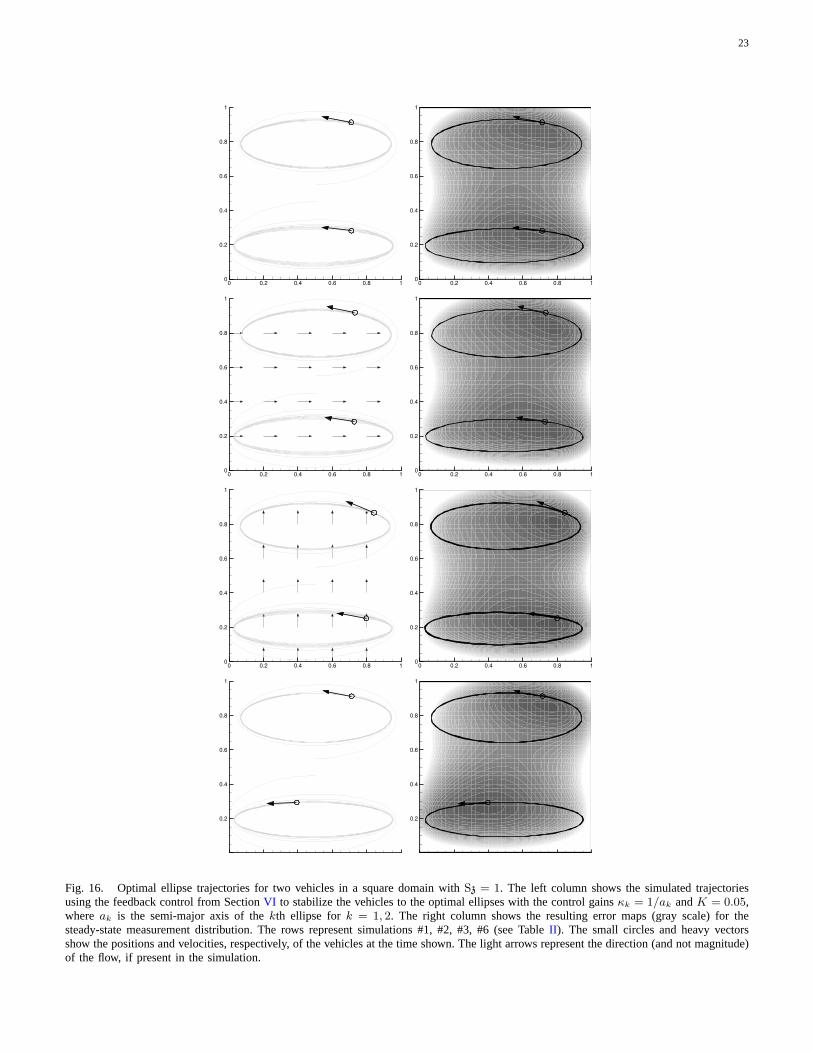
23

0.2

0.4

0.6

0.8

1

0 0.2 0.4 0.6 0.8 10

0.2

0.4

0.6

0.8

1

0 0.2 0.4 0.6 0.8 10

0.2

0.4

0.6

0.8

1

0 0.2 0.4 0.6 0.8 10

0.2

0.4

0.6

0.8

1

0 0.2 0.4 0.6 0.8 10

0.2

0.4

0.6

0.8

1

0 0.2 0.4 0.6 0.8 10

0.2

0.4

0.6

0.8

1

0 0.2 0.4 0.6 0.8 10

0.2

0.4

0.6

0.8

1

0.2

0.4

0.6

0.8

1

Fig. 16. Optimal ellipse trajectories for two vehicles in a square domain withSz = 1. The left column shows the simulated trajectoriesusing the feedback control from SectionVI to stabilize the vehicles to the optimal ellipses with the control gainsκk = 1/ak andK = 0.05,whereak is the semi-major axis of thekth ellipse fork = 1, 2. The right column shows the resulting error maps (gray scale) for thesteady-state measurement distribution. The rows represent simulations #1, #2, #3, #6 (see TableII ). The small circles and heavy vectorsshow the positions and velocities, respectively, of the vehicles at the time shown. The light arrows represent the direction (and not magnitude)of the flow, if present in the simulation.

24

Sim Flow direction Heading Coupling Metric#1 N/A on 0.018#2 0o on 0.020#3 90o on 0.054#4 180o on 0.023#5 270o on 0.101#6 N/A off 0.236

TABLE II

METRIC FOR SIMULATED OPTIMAL TRAJECTORIES.

The metric is the integral of the squared error over the domain, so

the trajectories with a smaller value of the metric are more

desirable.

contradicted our intuition that high eccentricity vehicletrajectories should not be aligned with the prevailingcurrents.

2) Role of Heading Synchronization:Clearly, the abil-ity of the controller to maintain the “synchronization”of the vehicles is, in large part, responsible for theperformance achieved by simulations #1, #2 and #4. Todemonstrate the influence of the synchronization, a sim-ulation was run without the heading coupling describedin Section VI . The performance for such an array isdramatically worse than the synchronized case. TableIIshows that, without heading coupling, the network ofvehicles performs even worse in the absence of currentsthan the synchronized array in the presence of currents.

VIII. F INAL REMARKS

We present developments on the design of mobilesensor networks that optimize sampling performance de-fined in terms of uncertainty in an estimate of a sampledfield over a fixed area. The general problem that we pose,and thus, the methodology that we develop, pertains tomobile sensor networks in a number of domains: land,air, space and underwater.

We address a number of general issues as well assome of the particular issues that distinguish mobilesensor networks in the ocean. For example, we make oursolutions robust to strong currents that can push aroundslow moving mobile sensors by determining optimalsolutions in the presence of currents, choosing solutionswith performance robust to small deviations and design-ing feedback control to stably coordinate vehicles.

We determine optimal, coordinated trajectories ofmobile sensors over a parameterized family of trajec-tories. This family consists of multiple closed curves(we specialize to ellipses), each with multiple sensorsmoving at constant speed. The relative positions of thesensors on these curves are parameterized by relativephases. This low-dimensional parameterization simpli-

fies the optimization problem and motivates the coordi-nated feedback control laws that include terms modeledafter coupled phase oscillator dynamics.

We present optimal solutions in several cases. Forexample, two sensors, each moving around a differentellipse, are optimized when their phases are synchro-nized. Sampling performance is significantly enhancedfor the closed-loop system with the coordinating feed-back control enabled. In the presence of a constant flowfield, the solution (with feedback control) with the majoraxes of the two ellipses aligned with the flow provideshigher performance than in the case the flow is alignedwith the minor axes of the ellipses.

In related work we are investigating inhomoge-neous statistics and alternative methods for computingand adapting the sampling metric. We are developingmethodology to further treat and exploit the flow field,to address a range of scales in the sampled field ofinterest and to make use of a heterogeneous sensornetwork. We are also investigating how well the dataset that optimizes the coverage metric presented in thispaper serves the needs of specific high resolution oceanforecasting models.

We describe in the paper a number of practical andcritical challenges of operating mobile sensor networksin the ocean: limitations on communication, computingand control, including inherent asynchronicities and la-tencies. We discuss how we have handled these chal-lenges in previous field work. However, these and otherproblems related to time and energy optimality remainoutstanding open problems of great interest.

Up until recently, our focus has been the optimal de-sign for Eulerian data assimilation. Recent developmentsin data assimilation extend this concept to Lagrangiandata assimilation [55], [56]. In a Lagrangian assimilationscheme, the paths of passive tracers or drifters (asopposed to an estimate of the Eulerian velocity) areassimilated directly into the ocean model. Although itwas developed for float data [57], [56], Lagrangian dataassimilation represents an exciting application for quasi-Lagrangian (i.e., weakly propelled) gliders. In particular,a Lagrangian metric and corresponding optimal trajecto-ries could be substituted into the usual objective analysisscheme.

IX. A CKNOWLEDGMENTS

This paper has greatly benefited from many enlight-ening discussions with Pierre Lermusiaux (Harvard Uni-versity), Eddie Fiorelli, Pradeep Bhatta, Fumin Zhangand Spring Berman (Princeton University) and RalfBachmayer (National Research Council of Canada).

25

Figure 4 was provided by Eddie Fiorelli, PradeepBhatta and Ralf Bachmayer. The authors are grateful toEddie Fiorelli and Fumin Zhang (Princeton University)for sharing their latests advances in formation design andcontrol.

This research was funded in part by Office of NavalResearch grants N0014-02-1-0826 and N00014–02–1–0861 and N00014–04–1–0534 and in part by the BelgianProgram on Inter-university Poles of Attraction, initiatedby the Belgian State, Prime Minister’s Office for Science,Technology and Culture. Derek Paley was supported bya National Science Foundation Graduate Research Fel-lowship, the Princeton Gordon Wu Graduate Fellowshipand the Pew Charitable Trust Grant 2000-002558.

APPENDIX

SHAPE DYNAMICS FOR ELLIPTICAL CONTROL

We first derive the dynamics of a single vehicle inthe coordinates(ρ, ρ′, ψ, ψ′, θ). Differentiating the defi-nitions (27) and (28) using R0 = µ0 = 0 and applyingthe model (12) for a single vehicle gives

d = ρei(ψ+µ0) + iρei(ψ+µ0)ψ = eiθ (47)

d′ = ρ′ei(ψ′+µ0) + iρ′ei(ψ

′+µ0)ψ′ = eiθ. (48)

Identifying the real and imaginary terms of (47) and (48)produces the system of equations,

ρ = cos(θ − µ0 − ψ) (49)

ρ′ = cos(θ − µ0 − ψ′) (50)

ψ =1ρ

sin(θ − µ0 − ψ) (51)

ψ′ =1ρ′

sin(θ − µ0 − ψ′) (52)

θ = u. (53)

In shape coordinates(ξ, η, α, β, λ), the system of equa-tions (49)-(53) becomes

ξ =12(sin(β+λ)− sin(β−λ)) = cosβ sinλ (54)

η =12(sin(β+λ) + sin(β−λ)) = sinβ cosλ (55)

α =12

(1

ξ+ηcos(β+λ) +

1ξ−η

cos(β−λ))

(56)

β =12

(1

ξ+ηcos(β+λ)− 1

ξ−ηcos(β−λ)

)(57)

λ = α− u. (58)

REFERENCES

[1] S. T. Besiktepe, P. F. J. Lermusiaux, and A. R. Robinson,“Coupled physical and biogeochemical data-driven simulationsof Massachusetts Bay in late summer: Real-time and postcruisedata assimilation,”Journal of Marine Systems, vol. 40, pp. 171–212, 2003.

[2] P. F. J. Lermusiaux, C. Evangelinos, R. Tian, P. J. Haley, J. J.McCarthy, N. M. Patrikalakis, A. R. Robinson, and H. Schmidt,“Adaptive coupled physical and biogeochemical ocean predic-tions: A conceptual basis,” inComputational Science - ICCS2004, Part 3, ser. Lecture Notes in Computer Science, vol. 3038,2004, pp. 685–692.

[3] J. D. Paduan and L. K. Rosenfeld, “Remotely sensed surfacecurrents in Monterey Bay from shore-based HF radar (coastalocean dynamics application radar),”Journal of GeophysicalResearch – Oceans, vol. 101, no. C9, pp. 20 669–20 686, 1996.

[4] P. F. J. Lermusiaux, “Estimation and study of mesoscale vari-ability in the Strait of Sicily,” Dynamics of Atmosphere andOceans, vol. 29, no. 2-4, pp. 255–303, 1999.

[5] C. H. Pilskaln, C. Lehmann, J. B. Paduan, and M. W. Silver,“Spatial and temporal dynamics in marine aggregate abundance,sinking rate and flux: Monterey Bay, central California,”Deep-Sea Research Part II-Topical Studies in Oceanography, vol. 45,no. 8-9, pp. 1803–1837, 1998.

[6] W. F. Dabberdt and T. W. Schlatter, “Research opportunitiesfrom emerging atmospheric observing and modeling capabili-ties,” Bulletin of the American Meteorological Society, vol. 77,no. 2, pp. 305–323, 1996.

[7] A. C. Lorenc, R. S. Bell, and B. Macpherson, “Themeteorological-office analysis correction data assimilationscheme,”Quarterly Journal of the Royal Meteorological So-ciety, vol. 117, no. 497, pp. 59–89, 1991.

[8] C. B. Paris, R. K. Cowen, K. M. M. Lwiza, D. P. Wang, andD. B. Olson, “Multivariate objective analysis of the coastalcirculation of Barbados, West Indies: Implication for larvaltransport,” Deep-Sea Research Part I – Oceanographic Re-search Papers, vol. 49, no. 8, pp. 1363–1386, 2002.

[9] J. Willcox, J. Bellingham, Y. Zhang, and A. Baggeroer, “Perfor-mance metrics for oceanographic surveys with autonomous un-derwater vehicles,”IEEE Journal Oceanic Engineering, vol. 26,no. 4, pp. 711–725, 2001.

[10] A. L. Bertozzi, M. Kemp, and D. Marthaler, “Determiningenvironmental boundaries: Asynchronous communication andphysical scales,” inCooperative Control, A Post-WorkshopVolume: 2003 Block Island Workshop on Cooperative Control,V. Kumar, N. Leonard, and A. Morse, Eds. Springer, 2005,pp. 35–42.

[11] D. Marthaler and A. L. Bertozzi, “Tracking environmental levelsets with autonomous vehicles,” inRecent Developments in Co-operative Control and Optimization, S. Butenko, R. Murphey,and P. Pardalos, Eds. Kluwer Academic Publishers, 2003.

[12] F. Zhang and N. E. Leonard, “Generating contour plots usingmultiple sensor platforms,” inProceedings of the IEEE SwarmIntelligence Symposium, 2005.

[13] E. Fiorelli, N. E. Leonard, P. Bhatta, D. Paley, R. Bachmayer,and D. Fratantoni, “Multi-AUV control and adaptive samplingin Monterey Bay,” in Proceedings IEEE AUV 2004: Workshopon Multiple AUV Operations, 2004, and to appear inIEEEJournal of Oceanic Engineering, 2006.

[14] A. Eliassen, J. S. Sawyer, and S. J., “Upper air networkrequirements for numerical weather prediction,”Technical Noteof the World Meteorological Organization, vol. 29, 1954.

[15] L. S. Gandin,Gidrometerologicheskoe Izdatelstvo – ObjectiveAnalysis of Meteorological Fields. Leningrad, Jerusalem: En-glish Translation by Israeli Program for Scientific Translations,1963.

[16] F. P. Bretherton, R. E. Davis, and C. B. Fandry, “A techniquefor objective analysis and design of oceanographic experimentsapplied to MODE-73,”Deep-Sea Research, vol. 23, pp. 559–582, 1976.

[17] C. H. Pilskaln, J. B. Paduan, F. P. Chavez, R. Y. Anderson, andW. M. Berelson, “Carbon export and regeneration in the coastal

26

upwelling system of Monterey Bay, central California,”Journalof Marine Research, vol. 54, no. 6, pp. 1149–1178, 1996.

[18] T. Hirawake, T. Odate, and M. Fukuchi, “Long-term variationof surface phytoplankton chlorophylla in the southern oceanduring 1965-2002,”Geophysical Research Letters, vol. 32, no.5 – L05606, 2005.

[19] D. K. Steinberg, M. W. Silver, C. H. Pilskaln, S. L. Coale, andJ. B. Paduan, “Midwater zooplankton communities on pelagicdetritus (giant larvacean houses) in Monterey Bay, California,”Limnology and Oceanography, vol. 39, no. 7, pp. 1606–1620,1994.

[20] J. Bellingham, “New oceanographic uses of autonomous under-water vehicles,”Marine Technology Society Journal, vol. 31,no. 3, pp. 34–47, 1997.

[21] T. B. Curtin, J. G. Bellingham, J. Catipovic, and D. Webb, “Au-tonomous oceanographic sampling networks,”Oceanography,vol. 6, no. 3, pp. 86–94, 1993.

[22] J. Sherman, R. E. Davis, W. B. Owens, and J. Valdes, “The au-tonomous underwater glider ‘Spray’,”IEEE Journal of OceanicEngineering, vol. 26, no. 4, pp. 437–446, 2001.

[23] D. Webb, P. Simonetti, and C. Jones, “SLOCUM: An under-water glider propelled by environmental energy,”IEEE JournalOceanic Engineering, vol. 26, no. 4, pp. 447–452, 2001.

[24] C. C. Eriksen, T. J. Osse, T. Light, R. D. Wen, T. W. Lehmann,P. L. Sabin, J. W. Ballard, and A. M. Chiodi, “Seaglider: Along range autonomous underwater vehicle for oceanographicresearch,”IEEE Journal of Oceanic Engineering, vol. 26, no. 4,pp. 424–436, 2001.

[25] D. Steere, A. Baptista, D. McNamee, C. Pu, and J. Walpole,“Research challenges in environmental observation and fore-casting systems,” inProceedings 6th International ConferenceMobile Computing and Networking (MOBICOMM), 2000.

[26] R. Cardell-Oliver, K. Smettem, M. Krantz, and K. Meyer, “Fieldtesting a wireless sensor network for reactive environmentalmonitoring,” in International Conference on Intelligent Sensors,Sensor Networks and Information Processing ISSNIP-04, 2004.

[27] Autonomous Ocean Sampling Network, MBARI website:http://www.mbari.org/aosn, 2003.

[28] D. L. Rudnick, R. E. Davis, C. C. Eriksen, D. M. Fratantoni, andM. J. Perry, “Underwater gliders for ocean research,”MarineTechnology Society Journal, vol. 38, no. 1, pp. 48–59, 2004.

[29] P. Ogren, E. Fiorelli, and N. E. Leonard, “Cooperative controlof mobile sensor networks: Adaptive gradient climbing ina distributed environment,” IEEE Transactions on AutomaticControl, vol. 49, no. 8, pp. 1292–1302, 2004.

[30] E. Fiorelli, P. Bhatta, N. E. Leonard, and I. Shulman, “Adaptivesampling using feedback control of an autonomous underwaterglider fleet,” in Proceedings of Symposium on Unmanned Un-tethered Submersible Technology, 2003.

[31] J. Graver, “Underwater gliders: Dynamics, control and design,”Ph.D. dissertation, Princeton University, 2005.

[32] P. F. J. Lermusiaux and A. R. Robinson, “Data assimilationvia error subspace statistical estimation. Part I: Theory andschemes,”Monthly Weather Review, vol. 127, no. 7, pp. 1385–1407, 1999.

[33] P. E. Lermusiaux, “Data assimilation via error subspace statis-tical estimation. Part II: Middle Atlantic Bight shelfbreak frontsimulations and ESSE validation,”Monthly Weather Review,vol. 127, no. 7, pp. 1408–1432, 1999.

[34] I. Shulman, C. R. Wu, J. K. Lewis, J. D. Paduan, L. K.Rosenfeld, J. C. Kindle, S. R. Ramp, and C. A. Collins, “Highresolution modeling and data assimilation in the Monterey Bayarea,” Continental Shelf Research, vol. 22, no. 8, pp. 1129–1151, 2002.

[35] P. F. J. Lermusiaux, “Uncertainty estimation and prediction for

the interdisciplinary ocean,”Journal of Computational Physics,submitted, 2005.

[36] I. Shulman, D. J. McGillicuddy, M. A. Moline, S. H. D. Had-dock, J. Kindle, D. Nechaev, and M. W. Phelps, “Biolumine-seence intensity modeling and sampling strategy optimization,”Journal of Atmospheric and Oceanic Technology, vol. 22, pp.1267–1281, 2005.

[37] S. R. Ramp, J. D. Paduan, I. Shulman, J. Kindle, F. L. Bahr, andF. Chavez, “Observations of upwelling and relaxation events inthe Northern Monterey Bay during august 2000,”Journal ofGeophysical Research – Oceans, vol. 110, Art. No. C07013,2005.

[38] T. Inanc, S. Shadden, and J. Marsden, “Optimal trajectory gen-eration in ocean flows,” inProceedings 43rd IEEE ConferenceDecision and Control, 2004.

[39] S. Berman, “Development of thermocline tracking capabilitiesfor the Slocum underwater glider,” Princeton University, Tech.Rep., 2004.

[40] P. F. J. Lermusiaux, D. G. M. Anderson, and C. J. Lozano,“On the mapping of multivariate geophysical fields: Error andvariability subspace estimates,”Quarterly Journal of the RoyalMeteorological Society, vol. 126, no. 565, pp. 1387–1429, 2000.

[41] P. F. J. Lermusiaux, “On the mapping of multivariate geophys-ical fields: Sensitivities to size, scales, and dynamcs,” Journalof Atmospheric and Oceanic Technology, vol. 19, no. 10, pp.1602–1637, 2002.

[42] A. Bennett, Inverse modeling of the ocean and atmosphere.Cambridge: Cambridge University Press, 2002.

[43] E. Kalnay,Atmospheric modeling, data assimilation, and Pre-dictability. Cambridge: Cambridge University Press, 2003.

[44] B. Grocholsky, “Information-theoretic control of multiple sen-sor platforms,” Ph.D. dissertation, The University of Sydney,2002, available from http://www.acfr.usyd.edu.au.

[45] A. S. Bower, D. M. Fratantoni, W. E. Johns, and H. Peters,“Gulf of Aden eddies and their impact on Red Sea water,”Geophysical Research Letters, vol. 29, pp. 21–1, Nov. 2002.

[46] R. Sepulchre, D. Paley, and N. E. Leonard, “Collective motionin the plane, part I: All-to-all communication,” 2005, acceptedfor publication inIEEE Transactions on Automatic Control.

[47] D. Paley, N. E. Leonard, and R. Sepulchre, “Oscillator modelsand collective motion: Splay state stabilization of self-propelledparticles,” in Proceedings 44th IEEE Conference Decision andControl, 2005.

[48] D. Paley, N. Leonard, and R. Sepulchre, “Collective motion:Bistability and trajectory tracking,” in Proceedings 43rd IEEEConference Decision and Control, 2004.

[49] D. Hilbert and S. Cohn-Vossen,Geometry and the Imagination,2nd ed. Chelsea Pub. Co., 1999.

[50] E. Buckingham, “On physically similar systems; illustrations ofthe use of dimensional equations,”Physical Review, vol. 4, pp.345–376, 1914.

[51] H. J. Thiebaux, “Experiment with correlation representationsfor objective analysis,”Monthly Weather Review, vol. 103, pp.617–627, 1975.

[52] ——, “Anisotropic correlation functions for objective analysis,”Monthly Weather Review, vol. 104, pp. 994–1002, 1976.

[53] W. Curtis, J. Logan, and W. Parker, “Dimensional analysis andthe Π theorem,”Linear Algebra and Applications, vol. 47, pp.117–126, 1982.

[54] S. Berman, “Estimation of ocean field decorrelation scalesfor the design of underwater glider sampling trajectories,”Undergraduate Senior Thesis, Princeton University, Princeton,2005.

[55] K. Ide, L. Kuznetsov, and C. K. R. T. Jones, “Lagrangian dataassimilation for point vortex systems,”Journal of Turbulence,vol. 3, p. Art. No. 053, 2002.

27

[56] A. Molcard, A. Griffa, and T. M. Ozgokmen, “Lagrangian dataassimilation in multilayer primitive equation ocean models,”Journal of Atmospheric and Oceanic Technology, vol. 22, no. 1,pp. 70–83, 2005.

[57] A. Molcard, L. I. Piterbarg, A. Griffa, T. M. Ozgokmen, andA. J. Mariano, “Assimilation of drifter observations for thereconstruction of the Eulerian circulation field,”Journal ofGeophysical Research – Oceans, vol. 108, no. C3, Art. No.3056, 2003.