
Collective Labour Supply: Heterogeneity and Non …uctp39a/BCMM.pdflective restrictions on labour...
29
Review of Economic Studies (2007) 74, 417–445 0034-6527/07/00150417$02.00 c 2007 The Review of Economic Studies Limited Collective Labour Supply: Heterogeneity and Non-Participation RICHARD BLUNDELL University College London and Institute for Fiscal Studies PIERRE-ANDRE CHIAPPORI University of Chicago and Columbia University THIERRY MAGNAC GREMAQ and IDEI, Université des Sciences Sociales and COSTAS MEGHIR University College London and Institute for Fiscal Studies First version received February 2003; final version accepted September 2006 (Eds.) We present identification and estimation results for the “collective” model of labour supply in which there are discrete choices, censoring of hours, and non-participation in employment. We derive the col- lective restrictions on labour supply functions and contrast them with restrictions implied by the usual “unitary” framework. Using the large changes in the wage structure between men and women in the U.K. over the last two decades, we estimate a collective labour supply model for married couples without chil- dren. The estimates of the sharing rule show that male wages and employment have a strong influence on bargaining power within couples. 1. INTRODUCTION The standard unitary labour supply model is unable to explain a number of empirical facts. First, the assumption of income pooling, where the source of income does not matter for house- hold behaviour is rejected (see, for instance, Thomas, 1990; Duflo, 2003; and the consider- able literature on intrahousehold allocation). Second, the compensated substitution effects be- tween male and female leisures, whenever compared are found not to be symmetric. Finally, many recent studies have recognized that a lot of inequality may be hidden within households and the standard unitary model cannot handle this issue by construction. Both the empirical failings and intrahousehold inequality concerns lead directly to the question of how resources are allocated within households and how this is likely to change in response to changes in the environment. When it comes to welfare assessment, policy evaluation, and cost–benefit analysis, intra- household allocation is a crucial issue for several reasons. First, to the extent that policy-makers are interested in individual well-being, analysis focusing on the interhousehold level may be insufficient, if not misleading. One can easily find examples in which a policy, say, slightly ame- liorates the well-being of poorest households, but at the cost of a large increase in intrahousehold disparities—so that, in the end, poorest individuals are made significantly worse off. Disregard- ing these issues (or dismissing intrahousehold inequality issues as irrelevant) may thus lead to important policy errors. 417
Transcript of Collective Labour Supply: Heterogeneity and Non …uctp39a/BCMM.pdflective restrictions on labour...

Review of Economic Studies (2007) 74, 417–445 0034-6527/07/00150417$02.00c© 2007 The Review of Economic Studies Limited
Collective Labour Supply:Heterogeneity and Non-Participation
RICHARD BLUNDELLUniversity College London and Institute for Fiscal Studies
PIERRE-ANDRE CHIAPPORIUniversity of Chicago and Columbia University
THIERRY MAGNACGREMAQ and IDEI, Université des Sciences Sociales
and
COSTAS MEGHIRUniversity College London and Institute for Fiscal Studies
First version received February 2003; final version accepted September 2006 (Eds.)
We present identification and estimation results for the “collective” model of labour supply in whichthere are discrete choices, censoring of hours, and non-participation in employment. We derive the col-lective restrictions on labour supply functions and contrast them with restrictions implied by the usual“unitary” framework. Using the large changes in the wage structure between men and women in the U.K.over the last two decades, we estimate a collective labour supply model for married couples without chil-dren. The estimates of the sharing rule show that male wages and employment have a strong influence onbargaining power within couples.
1. INTRODUCTION
The standard unitary labour supply model is unable to explain a number of empirical facts.First, the assumption of income pooling, where the source of income does not matter for house-hold behaviour is rejected (see, for instance, Thomas, 1990; Duflo, 2003; and the consider-able literature on intrahousehold allocation). Second, the compensated substitution effects be-tween male and female leisures, whenever compared are found not to be symmetric. Finally,many recent studies have recognized that a lot of inequality may be hidden within householdsand the standard unitary model cannot handle this issue by construction. Both the empiricalfailings and intrahousehold inequality concerns lead directly to the question of how resourcesare allocated within households and how this is likely to change in response to changes in theenvironment.
When it comes to welfare assessment, policy evaluation, and cost–benefit analysis, intra-household allocation is a crucial issue for several reasons. First, to the extent that policy-makersare interested in individual well-being, analysis focusing on the interhousehold level may beinsufficient, if not misleading. One can easily find examples in which a policy, say, slightly ame-liorates the well-being of poorest households, but at the cost of a large increase in intrahouseholddisparities—so that, in the end, poorest individuals are made significantly worse off. Disregard-ing these issues (or dismissing intrahousehold inequality issues as irrelevant) may thus lead toimportant policy errors.
417

418 REVIEW OF ECONOMIC STUDIES
A second and more subtle problem is directly linked to a crucial insight of bargaining theory,namely that changes in outside options may have a strong impact on behaviour and welfareeven for agents who are not directly affected by these options. For instance, the availability ofunemployment benefits may affect the structure of the bargaining game between employers andemployees, hence the situation of workers who do not actually receive these benefits. In thesame vein, Haddad and Kanbur (1992), analysing the welfare impact of guaranteed employmentprogrammes in India, stress that these programmes, by generating credible outside options forwomen, may have a huge impact on intrahousehold allocation and the decision process. Theyargue that standard cost–benefit analysis, which exclusively concentrates on the gains receivedby agents who actually participate in the programme, may thus miss its major benefit, leading to abiased evaluation of its consequences. A third example, which lies at the core of the present paper,relates to the impact of wage increases on household behaviour. In the standard “unitary” model,wages matter in so far as they affect the household’s budget constraint; when a household memberis not working, changes in his/her “potential” wage cannot matter. Bargaining theory, on theother hand, suggests the opposite conclusion: if potential wages affect bargaining positions (say,because a member’s threat point involves participation in the labour market), then any variationin the potential wage of an unemployed member will modify the behaviour of (and the welfareallocation within) the household.
Clearly, these issues cannot be addressed within a unitary setting; a richer conceptual frame-work is needed, where individuals retain their identity within the household and where questionsof individual welfare make sense. The “collective” model of household behaviour provides pre-cisely such a framework. In this paper, we use and develop further the framework of Chiappori(1988) to estimate individual preferences and within-household allocation rules based on observ-able labour supply decisions of the household. As suggested by the above discussion, we areprimarily interested in participation decisions in general and the role of wages of unemployedmembers in particular.
To empirically analyse these important wage effects in a convincing way we use the largechanges in the wage structure between men and women over time in the U.K. to provide iden-tification of the labour supply model without relying on arbitrary exclusion restrictions or oncross-sectional variation in wages. In this empirical implementation we have to acknowledgecertain features of observed family supply decisions. First, women’s labour supply displays awide range of hours of work and a substantive fraction do not work. Second, that male laboursupply is discrete and does not fit the continuous choice paradigm provides a reasonable approx-imation for female labour supply in couples. These features provide a key motivation for theapproach we take to modelling collective labour supply in this paper.
1.1. Labour market participation and the collective model
An important motivation of our research is to disentangle the “bargaining” aspects involved inparticipation decisions from the more standard income and substitution effects. A careful studyof non-participation is crucial in this respect because the effect of changes in the potential wageof a non-participating member provides key insights into the bargaining process.
When analysing labour supply decisions of couples, the econometrician can allocate house-holds into four different regimes, defined by the interaction of participation decisions of bothspouses. Empirically, the information of interest is summarized by two “participation frontiers”between regimes of participation for both members, as functions of any relevant covariates.Moreover, conditional on participation, labour supply functions provide additional information.Clearly, the four regimes are not equally informative in terms of both testability and identifica-tion. For instance, not much in terms of additional identifying power should be expected when
c© 2007 The Review of Economic Studies Limited
BLUNDELL ET AL. COLLECTIVE LABOUR SUPPLY 419
considering the sample of households where both spouses do not work, since there are no otherpieces of information on behaviour in this regime. At the other extreme, the regime in whichboth spouses work has already been studied in the theoretical literature, from both a unitary anda collective perspective (Chiappori, 1988, 1992). This is the case where one should expect thestrongest identifying power for preferences and any other function of interest (such as sharingrules), provided that we can condition the empirical analysis on the participation decisions.
It is only recently that other work regimes have been investigated and this paper was the firstto propose such an analysis.1 Our study is based on survey data (UK Family Expenditure Survey(FES)) over a long time span—one of the few long-term surveys that allows for an empiricalanalysis of this type. As noted above, these data display two important features. First, a largeproportion of women do not work; when they do, however, the range of hours that they supplyis large. We thus have to discuss the implications of the collective framework when a good ison the corner. Second, although non-participation rates for men are large and approaching thosefor women over time, when men do work, they nearly always work full time. In our data-setpractically no men are seen to work for less than 35 hours a week and very few are seen to workfor less than 52 weeks. As we illustrate in the empirical section, modelling the small variationof hours above 35 hours a week or below 52 weeks a year does not seem to us to be the mostimportant issue to focus on.
These characteristics of the data lead to the basic methodological choices of our paper.Namely, we assume that the husband’s decision is discrete (work or not) and that only this di-mension of labour supply choice affects preferences. The collective framework we present thusbreaks new ground. First, identification cannot rely on both labour supplies being continuous.Second, female labour supply is shown to vary with male wages even when he is not working, al-though this relationship operates in a restrictive way that can be tested. Third, our extension of thecollective approach to discrete choices relies on an original assumption of “double indifference”towards labour market participation; we explore the theoretical foundations and the empiricalconsequences of this formalization on the collective approach and in particular on the way in-trahousehold allocation of resources operates in the neighbourhood of the participation frontiers.Finally, our model is not nested in the collective model with continuous hours (Chiappori, 1988)and thus extends the generality of the collective approach.
1.2. Identification
From an econometric point of view, we recognize the importance of unobserved heterogeneity,which in itself creates further difficult identification questions. We cannot analyse identificationin each regime of participation as in the original homogenous case of Chiappori (1988) as newselection and other endogeneity issues arise. We discuss estimation within the context of para-metric preference structures (i.e. linear or log-linear), and we show in the working paper versionthat given the functional form assumptions and exclusion restrictions, the restrictions originatingfrom the collective framework overidentify the model in a semi-parametric way.2 For simplicity,we use full parametric assumptions in the empirical analysis.
The framework we develop allows identification of preferences without using informa-tion on preferences for singles; we allow all parameters of the utility function to depend onwhether one is married or not. The surprising result, in this context, is that the collective frame-work implies restrictions on household labour supply, even when male labour supply is discrete.Modelling household formation and dissolution and identifying the way that marriage affects
1. For a related work, see Donni (2003).2. Working paper with proofs and detailed discussions of many of the issues is available at http://
www.ifs.org.uk/workingpapers/wp0119.pdf
c© 2007 The Review of Economic Studies Limited

420 REVIEW OF ECONOMIC STUDIES
preferences are of course other issues of critical importance. It is beyond the scope of this paper,although we view the present contribution as a crucial step in this direction.
In this paper, we select only couples without children because we do not allow for publicgoods or for household production in the theoretical model we consider. Individuals can careabout each other’s welfare, but not by the way in which this welfare is generated. These restric-tions would be particularly stringent in the presence of children, where the decisions on howmany resources should be devoted to them is of central importance and is reflected in day-to-dayflows in consumption. A clear implication is that our results are only directly valid for this groupof individuals. However, this is a valuable first step in our attempt to construct empirical modelsin the more complex context of the collective models.
1.3. Main findings
In this paper we use U.K. survey data (FES) for the years 1978–2001. Exploiting the largechanges in the wage structure in the U.K. over this period to provide identification in itself dis-tinguishes us from many other papers. Our results show that collective model is not rejected. Inthe collective model, the estimated female labour supply wage (respectively income) elasticity atmean wages is 0·3 (resp. −0·85), and these results conform well with previous results where theanalysis is conditioned on the male working.
In addition, new and interesting patterns emerge. Of particular interest, given the motiva-tions stated above, is the finding that female labour supply depends on male wage even whenthe husband is not working although the estimate is not precise. Moreover, the direction of thisrelationship goes exactly as predicted by a bargaining interpretation of the collective model. Amale wage increase when he is working expands the household’s total income, which in generalbenefits both members;3 through a standard income effect, female number of hours should bereduced, which is what we find. On the contrary, a male wage increase when he is idle has no im-pact on the household’s budget constraint, but influences the intrahousehold distribution of power.Indeed, we find that such an increase augments her working time, which suggests a reallocationof household resources in his favour. This result confirms the basic insights described above.
Finally, the estimation of the sharing rule implies that bargaining power is strongly affectedby male wages. One pound increase in his earnings when he is working increases his consumptionby about 0·88 of a pound, while he gets to keep 0·73 of an increase in unearned income. Whenhe does not work all these effects get compressed by 0·71 of their values implying a greater shiftof marginal resources to the wife.
1.4. Literature
There are relatively few empirical studies of family labour supply outside the unitary model. Anumber of more recent studies have used micro-data to evaluate the pooling hypothesis or torecover collective preferences using exclusive goods, but these studies typically look at privateconsumption rather than labour supply. For example, Thomas (1990) finds evidence against thepooling hypothesis by carefully examining household data from Brazil. Browning, Bourguignon,Chiappori and Lechene (1996) use Canadian household expenditure data to examine the poolinghypothesis and to recover the derivatives of the sharing rule. Clothing in this analysis is theexclusive good providing identification, rather than labour supply which is problematic for asample of couples without children who both work full time.
Recent empirical studies concerning family labour supply include Lundberg (1988), Kapteynand Kooreman (1992), Apps and Rees (1996), and Fortin and Lacroix (1997). Each of these aims
3. See Chiappori and Donni (2005) for a precise analysis of this issue.
c© 2007 The Review of Economic Studies Limited
BLUNDELL ET AL. COLLECTIVE LABOUR SUPPLY 421
to provide a test of the unitary model and to recover some parameters of collective preferences.Lundberg attempts to see which types of households, distinguished by demographic composition,come close to satisfying the hypotheses implied by the unitary model. The other three studies takethis a step further by directly specifying and estimating labour supply equations from a collec-tive specification. Apps and Rees (1996) specify a model to account for household production.Kooreman and Kapteyn (1990) use data on preferred hours of work to separately identify indi-vidual from collective preferences and, consequently, to identify the utility weight. Fortin andLacroix (1997) follow closely the Chiappori framework and allow the utility weight to be a func-tion of individual wages and unearned incomes. They use a functional form that nests both theunitary and the collective model as particular cases and find that the restrictions implied by theunitary setting are strongly rejected, while the collective ones are not. In a more recent paper,Chiappori, Fortin and Lacroix (2002) extend the collective model to allow for “distribution fac-tors”, defined as any variable that is exogenous with respect to preferences, but may influencethe decision process. Using Panel Study of Income Dynamics (PSID) data and choosing the sexratio as a distribution factor, they find that the restrictions implied by the collective model arenot rejected; furthermore, they identify the intrahousehold sharing rule as a function of wages,non-labour income, and the sex ratio. It is important to note that the latter works assume thatboth male and female labour supplies vary continuously. The case of discrete male labour supply,which raises particular difficulties, is a specific contribution of the current paper; however, Donni(2003) applies similar ideas to taxation. Of course, there are issues that we do not address; theseinclude uncertainty, inter-temporal considerations, taxation, and others. Some work has been car-ried out by Attanasio and Mazzocco (2001), Donni (2003), and Mazzocco (2003a,b, 2004). Moreis left for future research in this important field, which can build on our framework.4
We set up the homogenous model in Section 2 and discuss its identification, the collectiverestrictions, and the corresponding restrictions in the unitary model. In Section 3, we specifythe empirical model, report estimates, and tests of unitary and collective restrictions. We presentestimates of the sharing rule and labour supply functions when he works or not. In our finalsection, we discuss how the model can be generalized to take into account household productionand public goods. We draw on work we have been developing to discuss some new identificationresults as well as data requirements for this more general problem.
2. THEORETICAL FRAMEWORK
We now present the collective model for male and female labour supply with discrete male laboursupplies.5 We then show how, given wages, other income and possible other exogenous variables,we can recover individual preferences and the sharing rule, from observations of labour supplyof each individual. Our analysis is based on the assumption that within-household allocationsare efficient. This implies, among other things, that side-payments are possible. We view thisas quite a natural assumption to make when modelling relationships of married individuals. Itturns out that when preferences are egoistic or caring, this assumption is an identifying one.6
Preferences are defined over goods and non-market time. In the basic model, we assume thatboth these goods are private and that there is no household production. The extension to accountfor household production is discussed in the concluding section of the paper, where we also
4. Udry (1996) studies a related problem, namely the allocation of inputs to agricultural production in a developingcountry. He concludes that the decision process entails inefficiencies, in the sense that a different allocation between“male” and “female” crops could increase total production.
5. The analysis assumes that unemployment is a labour supply decision.6. Browning and Chiappori (1998) and Chiappori and Ekeland (2002) show that efficiency alone (with general
preferences) cannot provide testable restrictions upon behaviour unless the number of commodities is at least five; inaddition, even with more than four commodities preferences are not identifiable.
c© 2007 The Review of Economic Studies Limited

422 REVIEW OF ECONOMIC STUDIES
consider the case of public consumption. Although some of the assumptions underlying the basicmodel are restrictive, we think of it as best applying to the population of married couples withno children; children are likely to be the most important source of preference interdependence,which we choose to exclude for the moment.
The original Chiappori (1988) theorem relied on the idea that when allocations are efficient(as assumed) the marginal rates of substitution between members in a household are equalized.In our case, in which there is censoring and where one of the individuals faces discrete choice forone of the goods, the derivation of the implications of the collective setting has to follow a differ-ent logic. In what follows below, we present the model and its assumptions formally and deriverestrictions on labour supply functions. We finish the section by deriving similar restrictions ofthe unitary model.
2.1. The general collective labour supply model
2.1.1. Preferences and decision process. We consider a labour supply model withina two-member household; let hi and Ci denote member i’s labour supply (with i = m, f and0 ≤ hi ≤ 1) and consumption of a private Hicksian commodity C (with C f +Cm = C ), respec-tively. The price of the consumption good is set to 1. We assume preferences to be of “egoistic”type; that is, member i’s utility can be written as Ui (1 − hi ,Ci ), where Ui is continuously dif-ferentiable, strictly monotone, and strongly quasi-concave.7 Also, let w f ,wm , and y denote thefemale and male wage and the household’s non-labour income, respectively.
A common assumption in previous works on collective labour supply (Chiappori, 1988,1992; Fortin and Lacroix, 1997; Chiappori et al., 2002) was that both labour supplies could varycontinuously in response to fluctuations in wages and non-labour income. If hm and h f are twicedifferentiable functions of wages and non-labour income, then generically, the observation of hm
and h f allows to test the collective setting and to recover individual preferences and individualconsumptions of the private good up to an additive constant (Chiappori, 1988). Empirically,however, the continuity assumption is difficult to maintain. As shown in the empirical section,while female labour supply varies in a fairly continuous manner, male labour supply is essentiallydichotomous. A first purpose of this paper is precisely to show that the collective model impliesrestrictions in the case where one labour supply is constrained to take only two values.8 Hence weassume throughout the paper that member f can freely choose her working hours, while memberm can only decide to participate (then hm = 1) or not (hm = 0). Let P denote the participationset, that is, the set of wage–income bundles such that m does participate. Similarly, N denotesthe non-participation set and L is the participation frontier between P and N .
As the household is assumed to take Pareto-efficient decisions, there exists for any (w f ,wm, y), some um(w f ,wm, y) such that (hi ,Ci ) is a solution to the programme
maxh f ,hm ,C f ,Cm
U f [1−h f ,C f ]
U m [1−hm,Cm] ≥ um(w f ,wm, y)
C = w f h f +wmhm + y
0 ≤ h f ≤ 1, hm ∈ {0,1}.
(1)
7. The utility functions can be of the caring type: each individual may care about the overall welfare of theirpartner, so long as they do not care about how it comes about.
8. This set-up is not nested and does not nest the continuous model since choice sets are different. The analysiscould easily be extended to any discrete labour supply function; for instance, the choice might be between non-activity,part-time or full-time work. In our data, however, male part-time work is negligible.
c© 2007 The Review of Economic Studies Limited
BLUNDELL ET AL. COLLECTIVE LABOUR SUPPLY 423
The function um(w f ,wm, y) defines the level of utility that member m can command when therelevant exogenous variables take the values w f ,wm, y though the analysis can be conditioned onany other exogenous variable. Underlying the determination of um is some allocation mechanism(such as a bargaining model) that leads to Pareto-efficient allocations. We do not need to be ex-plicit about such a mechanism; hence the collective model does not rely on specific assumptionsabout the precise way that couples share resources.
Also, note that, in general, we allow um to depend on the husband’s wage even when thelatter does not work. The idea here is that within a bargaining context, his threat point may welldepend on the wage he would receive if he chose to work. If so, most cooperative equilibriumconcepts will imply that um is a function of both wages and non-labour income; in each case,indeed, a change in one of the threat points does modify the outcome. Regarding non-cooperativemodels of bargaining, various situations are possible. In some cases, for instance, the outcomedoes not depend on the threat points, which rules out any dependence of this kind. More interest-ing is the suggestion of MacLeod and Malcomson (1993), where the outcome of the relationshipremains constant when the threat points are modified, unless one individual rationality constraintbecomes binding; then the agreement is modified so that the resulting outcome “follows” themember’s reservation utility along the Pareto frontier.9 In our context, this implies that among allhouseholds where m is not working, only some will exhibit the dependence on m’s wage. Finally,note that preferences (and the Pareto weights) are allowed to depend on taste shifter variables,such as age, etc.
2.1.2. The participation decision: who gains, who loses? In the standard unitary frame-work, the participation decision is modelled in terms of a reservation wage. At this wage, theagent is exactly indifferent between working and not working. Generalizing this property to oursetting is however tricky, since now two people are involved. The most natural generalizationof the standard model is to define the reservation wage by the fact that one member (say, themember at stake, here the husband) is indifferent between working and not working. An impor-tant remark is that, in this case, Pareto efficiency requires that both members are indifferent. Tosee why, assume that the wife is not indifferent—say she experiences a strict loss if the husbanddoes not participate. Take any wage infinitesimally below the reservation wage and consider thefollowing change in the decision process: the husband does work and receives ε more (of theconsumption good) than previously planned. The husband is better off, since he was indifferentand he receives the additional ε and if ε is small enough, the wife is better off too, since the εloss in consumption is more than compensated by the discrete gain due to his participation.
In the remainder, we shall use the “double indifference” assumption, that can be formallystated as follows:
Definition and Lemma Double Indifference. The participation frontier L it is such thatmember m is indifferent between participating or not. Pareto efficiency then implies that f isindifferent as well.
Technically, this amounts to assuming that in the programme (1) above, um is a contin-uous function of both wages and non-labour income. Natural as it may seem, this continuityassumption still restricts the set of possible behaviour (and, as such, plays a key role for derivingrestrictions).
9. This will typically be the case for a generalization of the Nash bargaining concept to the case in which therelationship is non-binding, in the sense that each member may at each period choose to leave. See Ligon (2002) for anaxiomatic approach of dynamic Nash bargaining in a household context.
c© 2007 The Review of Economic Studies Limited

424 REVIEW OF ECONOMIC STUDIES
A possible, quite general interpretation is that the household first agrees on some general“rule” that defines, for each possible price–income bundle, the particular (efficient) allocationof welfare across members that will prevail. Then this rule is “implemented” through specificchoices, including m’s decision to participate. Although the latter is assumed discrete, it cannot,by assumption, lead to discontinuous changes in each member’s welfare, in the neighbourhoodof the participation frontier; on the contrary, the participation frontier will be defined preciselyas the locus of the price–income bundles such that m’s drop in leisure, when participating, canbe compensated exactly by a discontinuous increase in consumption that preserves smoothnessof each member’s well-being.
The double indifference assumption can be justified from an individualistic point of view.That both members should be indifferent sounds like a natural requirement, especially in a contextwhere compensations are easy to achieve via transfers of the consumption good. Conversely,a participation decision entailing a strict loss for one member is likely to be very difficult toimplement; all the more when the loss is experienced by the member who is supposed to startworking.
2.1.3. The sharing rules. It is well known that Pareto optima can be decentralized in aneconomy of this kind. Just as in Chiappori (1992), this property defines the central concept of thesharing rule. The important distinction here is that the decision of one of the members is discrete:the male can only decide to work or not.
Participation. Let us first consider the case when m does participate. His utility is thusU m(Cm,0), and we have
U m(Cm,0) = um(w f ,wm, y). (2)
Solving for consumption Cm we obtain
Cm = V m[um(w f ,wm, y)] = �(w f ,wm, y),
where V m is the inverse of the mapping U m(·,0). Function �(w f ,wm, y) is called the sharingrule. Now, Pareto efficiency is equivalent to f ’s behaviour being a solution of the programme
maxh f ,C f
U f [1−h f ,C f ]
C f = w f h f + y +wm −�(w f ,wm, y)
0 ≤ h f ≤ 1.
(3)
This generates a labour supply of the form
h f (w f ,wm, y) = H f [w f , y +wm −�(w f ,wm, y)], (4)
where H f is the Marshallian labour supply function associated with U f , which can be equal to0 if a corner solution arises.
A first consequence is that, for any (w f ,wm, y) ∈ P such that h f (w f ,wm, y) > 0:
1−�wm
1−�y= h f
wm
h fy
= A(w f ,wm, y). (5)
Note that in the absence of unobserved heterogeneity in preferences, the function h f andhence the ratio A are empirically observable. Hence (5) provides a first restriction of �.
c© 2007 The Review of Economic Studies Limited

BLUNDELL ET AL. COLLECTIVE LABOUR SUPPLY 425
Non-participation. We now consider the non-participation case. Then male’s utility isU m(Cm,1) and we have that
U m(Cm,1) = um(w f ,wm, y) = V −1m (�(w f ,wm, y)), (6)
which can be inverted in
Cm = W m[V −1m (�(w f ,wm, y))] = F(�(w f ,wm, y)), (7)
where W m is the inverse of the mapping U m(·,1) and where F = W m ◦ (V m)−1 is increasingbecause both V m and W m are increasing.
As before, f ’s decision programme leads to a labour supply of the form
h f (w f ,wm, y) = H f [w f , y − F(�(w f ,wm, y))], (8)
and for any (w f ,wm, y) ∈ N such that h f (w f ,wm, y) > 0:
−F ′�wm
1− F ′�y= h f
wm
h fy
=B(w f ,wm, y). (9)
Note that in contrast to the unitary model f ’s labour supply will depend on m’s (potential)wage even when m is not working because the decision process will vary with wm .10
It should finally be stressed that the function A (respectively B) is defined only on P(respectively N ), that is, for the set of wages and non-labour incomes for which the male works(does not work). Moreover, functions A and B are only defined when the female works.
2.1.4. The participation decision. The participation frontier L is defined by the set ofwages and non-labour income bundles (w f ,wm, y) ∈ L , for which m is indifferent betweenparticipating or not:
Lemma 1. The participation frontier L is characterized by
∀(w f ,wm, y) ∈ L , �(w f ,wm, y)− F(�(w f ,wm, y)) = wm . (10)
Proof. Since, on L , f is also indifferent between m participating or non-participating, itmust be the case that f ’s income does not change discontinuously in the neighbourhood of thefrontier. Since total income does change in a discontinuous way (net increase of wm when mparticipates), it must be the case that the whole gain goes to m. ‖
The Lemma shows that at the participation frontier all additional incomes from participationgo to m to compensate him for the discrete increase in his labour supply. This is a property thatdepends on all goods being private and may not hold in the presence of public goods as wediscuss in the last section, Extensions.
To parameterize L , we choose to use a shadow wage condition; that is, m participates if andonly if
wm > γ (w f , y),
for some γ that describes the frontier. Note that this reservation wage property does not stemfrom the theoretical set-up as in standard labour supply models, but has to be postulated. This
10. See Neary and Roberts (1980) on shadow prices when a good is at a corner.
c© 2007 The Review of Economic Studies Limited

426 REVIEW OF ECONOMIC STUDIES
will be true if (10) has a unique solution for wm , a sufficient condition for which it is a contractionmapping:11
Assumption R. The sharing rules are such that
∀(w f ,wm, y), |[1− F ′(�(w f ,wm, y))]�wm (w f ,wm, y)| < 1. (11)
In this case whenever h f > 0, γ is characterized by the following equation:
∀(w f , y), �(w f ,γ (w f , y), y)− F(�(w f ,γ (w f , y), y)) = γ (w f , y), (12)
which implies(�y +γy�wm ) = γy
(1− F ′)(13)
�w f = γw f
γy�y .
In the second equation, the relative effect of w f and y on the participation frontier is equal totheir relative effect in the sharing rule since it is only through that function that those variablesaffect male participation. In contrast, in the first equation, it is the absolute level of the effect ofy that allows identification of the first derivative of the utility difference (F ′) conditional on thesharing rule. Equations (5) and (9) complete the system as shown next.
2.1.5. Restrictions from the collective model. What are the restrictions implied by thecollective setting just described with private consumption? And is it possible to recover thestructural model—that is, preferences and the sharing rules—from observed behaviour?
Proposition 2. Under the conditions listed in the Appendix we have the following:
(i) The collective model with private commodities leads to restrictions on household behaviour.In particular on the frontier when she participates ( i.e. for the set of w f , wm, and y suchthat wm = γ (w f , y) and h f > 0) we have that
−�wm + A�y = A −1
−�wm + B�y = BF ′
γy�wm +�y = γy(1−F ′)
�w f = γw fγy
�y .
(14)
(ii) The preferences and the sharing rules can be recovered up to an additive constant every-where where h f > 0.
Proof.
(i) We have assumed that um(w f ,wm, y) is continuously differentiable everywhere. It followsthat both (5) and (9) are valid on the frontier as well. Hence, on the frontier, using (5), (9),and (13) the sharing rule is determined by (14).
11. In words consider the increase in m’s consumption resulting from an infinitesimal increase dwm in m’s wage.When m is participating, dwm increases both the household income and m’s bargaining power, while the first effect doesnot operate when m does not participate. Let dcm denote the consumption change in the former case and dcm∗ in thelatter. Then (11) states that the difference dcm −dcm∗ cannot be more than the initial increase dwm .
c© 2007 The Review of Economic Studies Limited

BLUNDELL ET AL. COLLECTIVE LABOUR SUPPLY 427
(ii) The proof follows in stages. First, we consider the restrictions, which recover the sharingrule and F ′ on the participation frontier. This is followed by a proof of identification outsidethe frontier. Identification of preferences then follows (see Appendix). Below we use theserestrictions to derive direct tests of the collective model.
These conditions can be interpreted as follows. The first condition is standard in the collec-tive framework; it expresses the fact that when he is working, his wage affects her labour supplyonly through an income effect. The second condition reflects the “structural stability” impliedby the collective setting. It states that what is determined by the couple’s decision process is theutility um(w f ,wm, y) he would reach for each wage–income bundle; this utility level being im-plemented by different consumption levels depending on whether he works or not. Finally, thelast two conditions reflect the “double indifference” property; they state that the participationfrontier is such that both he and she are indifferent between his working and not working.
2.2. Unitary model restrictions
In the previous sections, we have derived the conditions that the labour supply functions of thefemale f and the participation frontier of the male m must satisfy to be compatible with thecollective setting, when all goods are private. We now contrast this result to the unitary frameworkand discuss the extent to which the two models provide different predictions and testable impli-cations that would allow us to discriminate between the two hypotheses. Here, the household,as a whole, is assumed to maximize some unique utility function U H, subject to the standardbudget constraint
maxh f ,hm ,C
U H [1−hm,1−h f ,C]
C = w f h f +wmhm + y
0 ≤ h f ≤ 1, hm ∈ {0,1}.(15)
Two points are worth mentioning here:
• We do not impose separability. This means that the household’s preferences for f ’s leisureand total consumption may in general depend on whether m is working or not. Let V W andV N (respectively h f
W and h fN) denote the corresponding indirect utility functions when he
works and when he does not (respectively female labour supply).• Preferences, here, only depend on total consumption C ; we do not introduce C f and Cm
independently. This is a direct consequence of the Hicks composite commodity theorem:since C f and Cm have identical prices, they cannot be identified in this general setting.
When she participates (h f > 0), one can immediately derive two restrictions, namely
∂h fW
∂wm= ∂h f
W
∂ymale works, (16)
and∂h f
N
∂wm= 0 male does not work. (17)
These are standard restrictions in the unitary context. Equation (16) is the “income pooling”property: when m’s number of hours (conditional on participation) are constrained, a change inwm can only have an income effect upon f ’s labour supply. Equation (17), on the other hand,reflects the fact that the income effect of m’s wage must be 0 when he is not working.
c© 2007 The Review of Economic Studies Limited

428 REVIEW OF ECONOMIC STUDIES
Finally, m’s participation decision depends on the difference between the household’s (indi-rect) utility when he is working and when he is not:
hm = 1 ⇔ V W(w f , y +wm) ≥ V N(w f , y).
In particular, the participation frontier is characterized by
V W(w f , y +γ (w f , y)) = V N(w f , y).
Differentiating and using Roy’s identity gives that, on the frontier,
∂γ
∂w f= h f
N −h fW +h f
N∂γ
∂y. (18)
The last term on the R.H.S. corresponds to a standard income effect: a marginal increase dw f
of female wage has the same first-order effect upon participation as an increase of householdnon-labour income equal to h f
Ndw f . In addition, it also affects the cost of male participation dueto the reduction of female working time; this corresponds to the term in h f
N −h fW.
We can summarize these findings as follows:
Proposition 3. The functions γ, h fP , and h f
N are compatible with the unitary model if andonly if conditions (16)–(18) are satisfied.
2.3. The separable unitary model
To conclude this discussion, we ask what happens when, within the unitary setting, we introducethe same separability assumption as in the collective case? Formally, this amounts to assumingthat
U H [1−hm,1−h f ,Cm,C f ] = U H [U m (1−hm,Cm),U f (1−h f ,C f )],
where U m and U f are interpreted as individual utility functions. Note that, in this case, onecan introduce Cm and C f (instead of their sum), since the Hicksian composite good theorem nolonger applies (see Chiappori, 1988, for a precise statement).
In principle, this is a particular case of both the unitary model (since it corresponds to themaximization of a unique utility) and the collective model (since maximizing U H under budgetconstraint obviously generates Pareto-efficient outcomes). The problem, however, is that the formis now very strongly constrained. To see how, consider the assumption made above that, on thePareto frontier, both members are indifferent between participation and non-participation. Thisneed not be the case here. Interpreting the utility function from the perspective of the collectivemodel, the maximization of U H may, and will in general, lead to participation decisions whereone member is a strict loser, this loss being compensated (at the household level, as summarizedby U H) by a strict gain for the spouse.12 The key intuition is that, within the unitary setting,the marginal utility of income, as evaluated at the household level, is equated across members.This by no means implies that utility levels are compensated in any sense. One can expect thatthe additional income generated by the husband’s participation will be partially distributed to thewife, who because of the standard income effect, will both work less and consume more. Thisneed not always be the case, though, because the husband’s marginal utility of consumption ismodified when he participates (unless, of course, his preferences are separable in leisure andconsumption). But, in any case, there is no reason to expect bilateral indifference.
12. Of course, within the unitary model it does not make sense to talk about gainers and losers within the household,since the unit is the household and not its members.
c© 2007 The Review of Economic Studies Limited

BLUNDELL ET AL. COLLECTIVE LABOUR SUPPLY 429
This provides an interesting illustration of the restrictive nature of the unitary model. Froman individualistic point of view that both members should be indifferent sounds like a naturalrequirement, especially in a context where compensations are easy to achieve via transfers of theconsumption good. Conversely, a participation decision entailing a strict loss for one memberis likely to be very difficult to implement. As it turns out, however, assuming a constant utilityfunction essentially forbids an assumption of this kind; the model is not flexible enough withrespect to the decision process to allow for such extensions.
3. ESTIMATING FAMILY LABOUR SUPPLY
3.1. Data
The data we use are drawn from the U.K. Family Expenditure Surveys from 1978 to the firstquarter of 2001 inclusive. We restrict attention to households where both the male and the femaleare below 60 and the male over 22. We further restrict the sample to include households wherethe female is over 35. This allows us to focus on those households whose children have eitherleft or who are unlikely to have children rather than on households who may still be planningchildren. Our households represent between 10% and 12% of the population of all households,including singles, where the head is 23–59 years old. They also represent between 13% and 20%of all couples (married or cohabiting) with a head in that age range. This proportion has beenincreasing, reflecting the decline in fertility. We exclude the self-employed, since their hours ofwork are not measured.13 The analysis should be viewed as pertaining to this subpopulation. Allmonetary values are deflated by the U.K. retail price index and are expressed in 2001 prices.
3.2. Specification and identifying assumptions
The discussion up to now sets up the model without unobserved heterogeneity. Allowing for un-observed heterogeneity together with non-participation complicates matters and raises the issueof identifiability of the model from available data. The complications are compounded by the factthat preference heterogeneity will also reflect itself in the sharing rule. This is why, building uponthe empirical labour supply literature (see Blundell and MaCurdy, 1999), we write a simple butalready rich model where all structural functions (labour supply and sharing rule) are semi-loglinear and additive in the heterogeneity terms and where wages are endogenous. In estimationwe assume that the vector of random terms is multivariate normal.14 We discuss the exclusionrestrictions in the empirical analysis below.
We now write the equations of female hours, male participation, and male and female wages.These equations are “semi-structural” in the sense that the sharing rule has been replaced by itsexpression as a function of wages, income, and other exogenous variables though wages areendogenous.
3.2.1. Female hours of work. A semi-log specification for female labour supply is apopular form to use on British data (see Blundell, Duncan and Meghir, 1998, for example) and is
13. Other selections to eliminate extreme outliers and influential observations are the following: we exclude allthose who report leaving full-time education before 10 years of age, all those with asset income of more than £1000 aweek in real terms and all those whose total non-durable consumption per week is £1000 a week below total householdweekly earnings.
14. In the working paper version we show that the model is semi-parametrically identified, that is, given theexclusion restrictions and a joint i.i.d. assumption for the vector of errors no distributional assumption is required. Seehttp://www.ifs.org.uk/workingpapers/wp0119.pdf
c© 2007 The Review of Economic Studies Limited

430 REVIEW OF ECONOMIC STUDIES
never rejected by our data. Interaction effects have not proved to be important. Thus we write
h fit = A f
0t + Amwmit + A f logw
fi t + Ay yit
+A4educ fi t + A5age f
i t + A6educmit + A7agem
it +u1i t , (19)
where f denotes female and m denotes male, wf
i t denotes the hourly wage rate for the female,wm
it denotes the weekly earning for the male, and yit denotes other household (non-labour) in-come. We use the level of male earnings, rather than the log, since this allows us to nest theincome pooling hypothesis, where Am = Ay . The variable educi denotes education of member i ,measured as the age the person left full-time education. Note that preferences are allowed to de-pend on the age and education of both partners as well as on cohort (or equivalently time effectsas expressed by the inclusion of A f
0t ). These factors may affect preferences for work directly orindirectly through the sharing rule.
The parameters of the labour supply function will be different, depending on whether themale is working or not. Let (19) represent the labour supply function when the male is working.When he is not, the labour supply function is given by
h fit = a f
0t +amwmit +a f logw
fi t +ay yit
+d0t +a4educ f
i t +a5age fi t +a6educm
it +a7agemit +u0i t . (20)
3.2.2. Male participation. The latent index for male participation is also assumed semi-log linear:
pmit = bm
pt +bmmwm
it +bmf logw
fi t +bm
y yit
+ζ4educ fi t + ζ5age f
i t + ζ6educmit + ζ7agem
it +umit , (21)
where pmit is positive for male participants and negative (or 0) otherwise.
One can solve simply for wmit when pm
it = 0 to derive the male reservation earnings and theparameters of the frontier of participation. These are
γ f = −bmf
bmm
, γy = −bmy
bmm
. (22)
Because of the sharing rule, the male participation equation and the two female labour supplyequations will depend, in general, on the same set of variables.
3.2.3. Wage equations. We take a standard human capital approach to wages. However,we do not restrict the relative prices of the various components of human capital to remain con-stant over time. Hence
wmit = αm
0t +αm1t educm
it +αm2t agem
it +αm2t (agem
it )2 +um
wi t
logwf
i t = αf
0t +αf
1t educ fi t +α
f2t age f
i t +αf
2t (age fi t )
2 +u fwi t .
(23)
Note that wages do not depend on the characteristics of the partner. All coefficients are time-varying reflecting changes in the aggregate price of each component of human capital.
c© 2007 The Review of Economic Studies Limited
BLUNDELL ET AL. COLLECTIVE LABOUR SUPPLY 431
3.2.4. Non-labour income. We measure non-labour income as the difference betweenconsumption and total household earnings, that is, yit = consumption − w
fi t h
fi t − wm
it pmit . This
approach reduces measurement error and accounts for sources of wealth that we do not observe,but that matter for individual decisions, including pension wealth.15 This measure of unearnedincome is treated as endogenous, and we use predictions based on the reduced-form equation
yit = αy0t +α
y1t educy
i t +αy2t agem
it +αy3t (agem
it )2 +α
y4t age f
i t +αy5t (age f
i t )2 +ay
6tµi t +ay7tµ
2i t
+ay8tµ
2i t +
3∑k=1
ay8+k1(µi t − sk > 0)(µi t − sk)
3 +ay121(µi t > 0)+uyit ,
where µi t is asset income not including any welfare payments or other government transfers.Thus the instrument used here is asset income interacted with time (see the time-varying co-efficients) as well as education and age interacted with time as above. We have included thepolynomial and spline terms in µi t as well as an indicator for non-zero asset income to improvethe fit of this reduced form.
3.2.5. Stochastic specification and exclusion restrictions. We assume that all error terms(u f
1i t , u f0i t , um
it , umwi t , u f
wi t , uyit ) are jointly conditionally normal with constant variance (and in-dependent of education, age, other income, and time). The basic exclusion restriction written inthe labour supply equations above is that education–time interactions and age–time interactionsare excluded from these equations, implying that differences in the preferences and the sharingrule across education groups remain constant over time. Hence, identification of labour supplyof both partners does not rely on excluding education. It relies on the way that the returns toeducation have changed (see Blundell et al., 1998). The rank condition for identification is thatwages have changed differentially across education groups over time. That they have done so inthe U.K. is a well-established fact (for men see Gosling, Machin and Meghir, 2000).
In addition we need to assume that any changes in the institutional framework has not af-fected the sharing rule or the composition of those households differentially across educationgroups. The changing structure of benefits in particular can affect the structure of the sharingrule, since it changes the outside option for the two partners. If this is the case differentiallyacross education groups then the cohort–time–education interactions would not be excludable.It is part of our identifying assumptions that the sharing rule (as well as preferences) has notchanged differentially across these groups. One key concern may be changes in the divorce laws.The most important change in the law came in 1969—nine years before the start of our data. Thishad an immediate and large impact on the number of divorces. However since the start of oursample divorces have remained more or less constant. Nevertheless we still need to assume thatother institutional changes have not changed preferences and sharing rules differentially acrosseducation groups. However, we do allow for a general time effects in preferences and the sharingrule by including time dummies in the model, as well as permanent differences across educationgroups. Together with the age effects this allows for differences across cohorts, which will re-flect the impact of the institutional changes or other changes such as fertility differences acrosscohorts.
3.2.6. Restrictions from the collective and unitary models. Using the family laboursupply specification (19), (20), and (22), the restrictions on the collective model derived from
15. See MaCurdy (1983), Blundell and Walker (1986), Arellano and Meghir (1992), and Blundell et al. (1998)among others.
c© 2007 The Review of Economic Studies Limited

432 REVIEW OF ECONOMIC STUDIES
Proposition 1 may be written (see working paper) as
Am−amAy−ay
= − 1γy
(I)
A f −a fAy−ay
= γ fγy
(II).(24)
It is interesting to contrast these restrictions with the structural restrictions that would bederived in the unitary case. Using the same notation (upper and lower cases for the two regimes),we have to impose equations (16)–(18) on the frontier (wm = γ f logw f + γy y + zγz). The firsttwo yield
Am = Ay (I)
am = 0 (II).(25)
Using (18), the definition of the frontier and these two restrictions give
γ f = (1+γy)(a f logw f +ay y)− (A f logw f + Ay(y +wm)).
As this equation is valid only on the frontier for any w f and y, it is also an equation of thefrontier. Therefore, the following vectors are colinear:⎛
⎜⎝1
−γ f
−γy
⎞⎟⎠,
⎛⎜⎝
−Ay
(1+γy)a f − A f
(1+γy)ay − Ay
⎞⎟⎠.
Hence in the unitary model we have two additional restrictions, namely
(1+γy)(ay − Ay) = 0 (I)
Ayγ f = (1+γy)a f − A f (II).(26)
3.3. Estimation
First we estimate two reduced-form participation equations: one for men and one for women.These are obtained by substituting the wages from the structural participation equations. Theresulting equations have the form
pkit = βk
0t +βk1t educ f
i t +βk2t age f
i t +βk3t (age f
i t )2
+βk4t educm
it +βk5t agem
it + (βk6t agem
it )2 +βk
7t yi t + vki t , k = m, f. (27)
Thus we include all variables that determine wages of men and women as well as other incomeyit and we allow the coefficients to change over time. The changes in the coefficients for variablesthat determine wages reflect the changing coefficients in the wage equations.16
We then estimate the female log-hourly wage equation and the male weekly earnings equa-tions including the inverse Mills ratio ( for females only) obtained from the estimated participationequations (27). In this parametric approach the wage equation is identified from the exclusion ofother income and the spouse’s characteristics as well as from the normality assumption.17
16. The changing coefficient on other income is not implied directly by the structure of the model (and it is notnecessary for identification purposes). We allow this as an extra degree of flexibility.
17. We tested for zero skewness in both the male earnings equation and in the female log hourly wage equation,taking into account the selection. The t-statistics were 1·93 and 1·38, respectively. Hence the hypothesis is accepted inboth cases.
c© 2007 The Review of Economic Studies Limited
BLUNDELL ET AL. COLLECTIVE LABOUR SUPPLY 433
Using the estimated wage equations, we impute offered wages for all individuals in the data-set. The participation frontier is then estimated using a probit, which includes other income, theimputed wages, time effects, age, and education.
The likelihood function for female labour supply when the man is working and when thereare nW such observations is
logLW =nW∑i=1
{1(h fit < 0)logPr(pm
it > 0,h fit < 0)
+1(h fit > 0)[logPr(pm
it > 0)+ log f (h fit |pm
it > 0)]}. (28)
When the man is not working (nN observations) this becomes
logLN =nN∑i=1
{1(h fit < 0)logPr(pm
it < 0,h fit < 0)
+1(h fit > 0)[logPr(pm
it < 0)+ log f (h fit |pm
it < 0)]}. (29)
In the above, f (·) represents the conditional normal density function and 1(a) is the indicatorfunction that is equal to 1 when a is true and 0 otherwise.
The labour supply estimates that are obtained from this procedure do not satisfy exactlythe assumptions of the collective (or the unitary) model. We can then carry out a test of the nullhypothesis that the coefficients can be rationalized using the unitary model and/or the collectivemodel and derive the structural estimates.
3.4. Basic facts in the data and the wage equations
For this group of households there have been large changes in the male participation rates. On theother hand, participation has been relatively steady over these years for married women withoutchildren. This is shown in Figure 1. Male participation has dropped for most age groups acrosscohorts to a greater or lesser extent, but the decline is larger for those over the age of 50, whichis generally interpreted as an increase in early retirement. In Figure 2 we show life-cycle partic-ipation. Each line represents a separate date of birth cohort. The vertical distance between thelines shows the decline across cohorts and this is particularly pronounced at older ages. Declinesin participation take place from about the age of 40 (see also Meghir and Whitehouse, 1997).Over the sample period there is no state pension available before the age of 60 for women and65 for men; so this in itself, cannot explain the decline in participation at older ages or acrosscohorts. Of course, older individuals will have more wealth than younger ones and some willbe able to retire on disability benefit. Empirically we capture the effect of increased wealth byusing a consumption-based measure of non-labour income, which will be higher for those withmore assets and hence more consumption. We also include age effects in the labour supply ofboth partners. However, for a deeper treatment of this issue one would need to couch the collec-tive model within a dynamic framework and deal directly with issues of commitment in dynamicsettings and inter-temporal allocations.18
The wage equations include age and years of education interacted with time. The participa-tion equation contains in addition the education of both partners and other household incomes
18. See Mazzocco (2003b) for a treatment of some of these issues.
c© 2007 The Review of Economic Studies Limited

434 REVIEW OF ECONOMIC STUDIES
FIGURE 1
Proportion of married men and women employed by year
FIGURE 2
Male participation over the life cycle by cohort
excluding any welfare benefits, all interacted with time. The p-values for all the female educa-tion terms in the male participation equation is 0·44% while just for the male education–timeinteractions the p-value is 1·5%. The male education terms in the female participation equationhave a joint p-value of 0·62% and for the time interactions alone is 1·4%. The p-value for theunearned income terms in both participation equations is indistinguishable from 0 although there
c© 2007 The Review of Economic Studies Limited
BLUNDELL ET AL. COLLECTIVE LABOUR SUPPLY 435
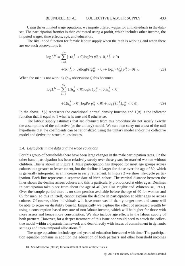
FIGURE 3
Actual and offered real log hourly wages for females by year
is less evidence that the effect varies over time since the p-value for the unearned income–timeinteractions is 15% in the male participation equation and 18% in the female one.
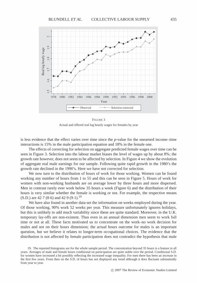
The effects of correcting for selection on aggregate predicted female wages over time can beseen in Figure 3. Selection into the labour market biases the level of wages up by about 8%; thegrowth rate however, does not seem to be affected by selection. In Figure 4 we show the evolutionof aggregate real male earnings for our sample. Following quite rapid growth in the 1980’s thegrowth rate declined in the 1990’s. Here we have not corrected for selection.
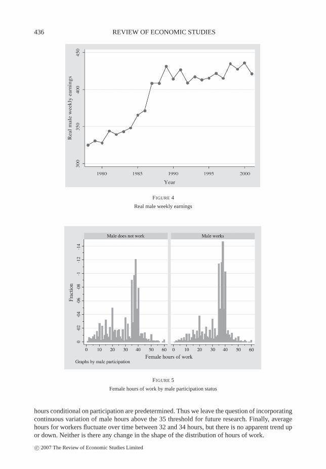
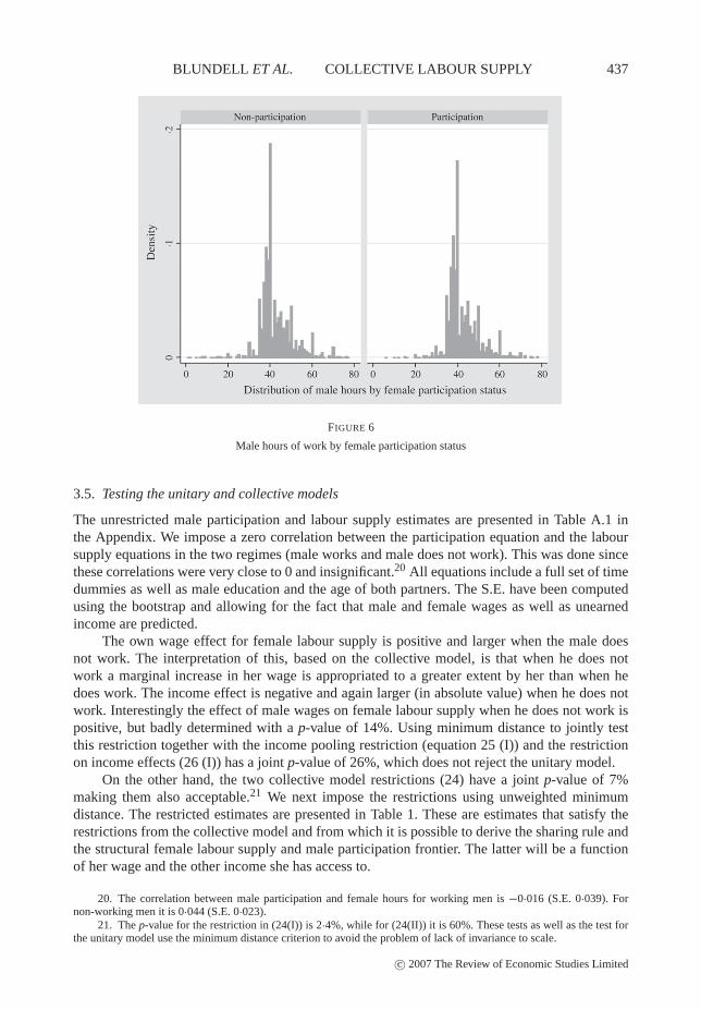
We now turn to the distribution of hours of work for those working. Women can be foundworking any number of hours from 1 to 55 and this can be seen in Figure 5. Hours of work forwomen with non-working husbands are on average lower by three hours and more dispersed.Men in contrast rarely ever work below 35 hours a week (Figure 6) and the distribution of theirhours is very similar whether the female is working or not. For example, the respective means(S.D.) are 42·7 (8·6) and 42·9 (9·1).19
We have also found in another data-set the information on weeks employed during the year.Of those working, 90% work 52 weeks per year. This measure unfortunately ignores holidays,but this is unlikely to add much variability since these are quite standard. Moreover, in the U.K.temporary lay-offs are non-existent. Thus even in an annual dimension men seem to work fulltime or not at all. These facts motivated us to concentrate on the work–no work decision formales and not on their hours dimension; the actual hours outcome for males is an importantquestion, but we believe it relates to longer-term occupational choices. The evidence that thedistribution is not affected by female participation does not contradict the hypothesis that male
19. The reported histograms are for the whole sample period. The concentration beyond 35 hours is a feature in allyears. Averages of male and female hours conditional on participation are quite stable over the period. Conditional S.D.for women have increased a bit possibly reflecting the increased wage inequality. For men there has been an increase inthe first few years. From then on the S.D. of hours has not displayed any trend although it does fluctuate substantiallyfrom year to year.
c© 2007 The Review of Economic Studies Limited
436 REVIEW OF ECONOMIC STUDIES
FIGURE 4
Real male weekly earnings
FIGURE 5
Female hours of work by male participation status
hours conditional on participation are predetermined. Thus we leave the question of incorporatingcontinuous variation of male hours above the 35 threshold for future research. Finally, averagehours for workers fluctuate over time between 32 and 34 hours, but there is no apparent trend upor down. Neither is there any change in the shape of the distribution of hours of work.
c© 2007 The Review of Economic Studies Limited
BLUNDELL ET AL. COLLECTIVE LABOUR SUPPLY 437
FIGURE 6
Male hours of work by female participation status
3.5. Testing the unitary and collective models
The unrestricted male participation and labour supply estimates are presented in Table A.1 inthe Appendix. We impose a zero correlation between the participation equation and the laboursupply equations in the two regimes (male works and male does not work). This was done sincethese correlations were very close to 0 and insignificant.20 All equations include a full set of timedummies as well as male education and the age of both partners. The S.E. have been computedusing the bootstrap and allowing for the fact that male and female wages as well as unearnedincome are predicted.
The own wage effect for female labour supply is positive and larger when the male doesnot work. The interpretation of this, based on the collective model, is that when he does notwork a marginal increase in her wage is appropriated to a greater extent by her than when hedoes work. The income effect is negative and again larger (in absolute value) when he does notwork. Interestingly the effect of male wages on female labour supply when he does not work ispositive, but badly determined with a p-value of 14%. Using minimum distance to jointly testthis restriction together with the income pooling restriction (equation 25 (I)) and the restrictionon income effects (26 (I)) has a joint p-value of 26%, which does not reject the unitary model.
On the other hand, the two collective model restrictions (24) have a joint p-value of 7%making them also acceptable.21 We next impose the restrictions using unweighted minimumdistance. The restricted estimates are presented in Table 1. These are estimates that satisfy therestrictions from the collective model and from which it is possible to derive the sharing rule andthe structural female labour supply and male participation frontier. The latter will be a functionof her wage and the other income she has access to.
20. The correlation between male participation and female hours for working men is −0·016 (S.E. 0·039). Fornon-working men it is 0·044 (S.E. 0·023).
21. The p-value for the restriction in (24(I)) is 2·4%, while for (24(II)) it is 60%. These tests as well as the test forthe unitary model use the minimum distance criterion to avoid the problem of lack of invariance to scale.
c© 2007 The Review of Economic Studies Limited

438 REVIEW OF ECONOMIC STUDIES
TABLE 1
Restricted labour supply estimates
Female labour supply—restricted estimates
Male works Male out of work
Male wage −0·50 0·48 2·64 2·46Female log wage 7·36 1·70 9·00 8·17Other income −1·13 0·14 −2·01 0·38
Asymptotic standard errors in italics.
As such, however, the estimates in Table 1 exhibit interesting patterns. The way the sign ofthe male wage effect on female labour supply changes with his work status is particularly note-worthy and can be given a bargaining interpretation: when he works, his wage has a negativeinfluence on her labour supply. This is the standard income effect, operating through intrahouse-hold transfers: an increase in male wages, when the husband is working, augments the house-hold’s total income and part of the enrichment is transferred to the wife. This income effect islarge enough to dominate bargaining effects; note, in particular, that the effect of an increase inhis wage when he works has the same sign as an increase in the household’s non-labour income,whether he works or not.22 However, when he is not working, the income effect of an increase inhis wage vanishes. The only consequence of a wage increase is a change in respective bargainingpowers, which must favour the husband. Consequently, we expect that he will attract a largerfraction of the (unchanged) household resources and by the same income effect as before, herlabour supply should now increase. This intuition is exactly confirmed by the data. In addition,the female wage effect is lower when he works than when he does not. The collective modelinterprets this as follows: when he works, for every pound that she earns she has to transfer anamount to him. This amount is lower when he does not work. Thus when he does not work anincrease in the wage gives her a larger incentive to increase hours of work. This is an implicationof equations (4), (8), and (11). It is particularly noteworthy that the patterns described above arepresent in the unrestricted estimates (see Table A.1 in the Appendix) and have not been producedsimply as a result of imposing the restrictions.
3.6. The estimates of the collective model
After imposing the restrictions above we check if a solution for the sharing rule exists. Thisdepends on whether the quadratic equation
φ2 + (−ay − Am +am)φ + Amay −am Ay = 0 (30)
has a solution for φ (see Proposition 1). One, two, or no solution may exist to equation (30).23
In our case the estimates imply two solutions. Generically, only at most one of the solutionsimplies an integrable well-behaved female labour supply. The solution shown below is the onethat satisfies Slutsky negativity as well as Assumption R.
The female labour supply implied by the estimates in the two samples we use is, up to aunidentified constant,24
h f = κ f + 13·07logw f − 4·20y f ,(29·0) (2·26)
(31)
22. That an increase in total non-labour income should necessarily be distributed between members is a standardconsequence of Nash bargaining; see Chiappori and Donni (2005).
23. Existence thus requires an additional (inequality) constraint that is verified here.24. In the equations that follow asymptotic S.E. are reported in parentheses below the estimated coefficients.
c© 2007 The Review of Economic Studies Limited

BLUNDELL ET AL. COLLECTIVE LABOUR SUPPLY 439
where y f is the other income allocated to the female member of the household, after the malehas been allocated his consumption. The income effect is precisely estimated, but the femalewage effect is badly determined. The implied wage elasticity is 0·33 while the income elasticityis 0·85, both evaluated at sample means. This labour supply satisfies the integrability conditionsof individual utility maximization, which, of course, is a requirement of the theory.
The estimates of the labour supply function and the participation frontier can be used toderive the implied sharing rules for when the husband works and when he does not. This is, ofcourse, a unique element of our approach, since it directly relates to the distribution of resourceswithin the household. For couples with a working husband and for the two samples we considerthese are
� = κ1 + 0·88wm − 1·36logw f + 0·73y.(0·13) (7·03) (0·15)
(32)
Thus an extra unit in male earnings implies an increase in his consumption by 0·88 units. Hekeeps 0·73 of a unit increase in household unearned income and he transfers 0·14 of a unit to herwhen her hourly wage rate increases by 10% (0·1 of a log point precisely), although this effect isnot well determined. The sharing rule when he is not working is given by
F(�) = κ0 + 0·71 (0·88wm − 1·36logw f + 0·73y),(0·25) (0·13) (7·03) (0·15)
(33)
and implies that all marginal increases get compressed by 71%.Thus the upshot of these results is that when he works, each tend to keep the larger part
of marginal increases in their respective incomes, and he keeps three-quarters of the increasesin unearned income. When he does not work he still obtains increases in consumption as hislabour market opportunities improve, but reduced to 71% of the previous values. The recentdecline in male participation would have reduced overall resources for households, but wouldalso imply a shift in available resources towards the woman. However, the effect of the femalewage on the sharing rule is very badly determined, limiting our ability to infer much about theimpact of increases in her wage. The impact of unearned income is however well determined anddemonstrates the difficulty of targeting women by increasing transfers to the household.
Finally, the implied participation frontiers based on the estimates for the two samples is
wrm = κm + 0·28y − 0·52logw f ,
(0·27) (2·76)(34)
but unfortunately the estimates are badly determined.Since his consumption grows with other income, increases in the latter increase his reser-
vation wage. However, increases in her wage reduce his consumption and hence make it morelikely that he works.
4. THE EXTENSION TO PUBLIC GOODS AND HOUSEHOLD PRODUCTION
4.1. The extension to public goods
Recent results show that an extension of the model to public consumption is feasible, althoughit may require additional information and/or particular assumptions. Not only are the main con-clusions of the private good setting (i.e. identification and testability) preserved in the extendedframework, but the current model can be interpreted, in this perspective, as the reduced form ofthe general problem, the emphasis being put here on private consumptions only. Although thesedevelopments are outside the scope of the present paper and will be the topic of future empiricalinvestigations, one can indicate the general flavour of these extensions. We summarize the state of
c© 2007 The Review of Economic Studies Limited
440 REVIEW OF ECONOMIC STUDIES
knowledge in this area which can be found in references made below and in Blundell, Chiapporiand Meghir (2005).
There are several ways of introducing public consumption within the collective model. Thesimplest manner, and perhaps the most natural one in the absence of price variation, is to assumethat the Hicksian good C is collectively consumed—that is, individual utilities are of the formUi (1− hi ,C). In this context, one can show (Chiappori and Ekeland, 2002, 2006; Donni, 2004)that the knowledge of individual labour supply functions generically allows exact identificationof the structural model, that is, preferences and Pareto weights, at least when the number of hoursis continuous (the extension to discrete participation, in the spirit of the present paper, is left forfurther research).
In a more general setting, public and private consumptions can be simultaneously consid-ered. Then difficult identification problems arise. While preferences over the private goods canreadily be identified conditional on the quantities consumed of the public goods, general identifi-cation typically requires additional information or more structure. A natural solution is to assumethat private consumption is separable, with member i’s utility of the form W i [ui (1−hi ,Ci ), K ](here K denotes public consumption, assumed observable).25 Even in the absence of price varia-tion (i.e. assuming that the price of both the public and the private goods is normalized to 1), thismodel is generically identifiable in a general, non-parametric sense: the observation of laboursupply and demand for public good as (continuous) functions of wages and non-labour incomeallows to uniquely recover the underlying structural model. Specifically, once the demand forpublic good is known, one can also recover the utility indices W i and the decision process, assummarized by the corresponding, individual Pareto weights.26 This first model can be extendedin different ways to include the case where the production of the public good also requires leisure.
Finally, an interesting perspective is provided in a recent contribution by Zhang and Fong(2001). In their model, leisure is partly private and partly public, in the sense that member i’sleisure (i = m, f ) can be written as Li = Li
p + L , where Lip represents i’s private leisure and
L is the common leisure of the couple. While individual labour supplies (hence total leisures)are observable, the allocation of time between private and public leisures is not. Under mildseparability assumptions, Zhang and Fong show the following result: if there exists a privategood (at least), the husband’s and the wife’s consumptions of which are independently observ-able, then the structural model (including the allocation of leisure between private and publictime) can be fully recovered. Again, this result suggest that data on private consumptions canhelp achieve identification of more general models, entailing private and public consumptions.As an example of such private consumption, one may think of clothing, as in Browning et al.(1996).
4.2. The extension to household production
In Blundell, Chiappori, Magnac and Meghir (2000), we discuss the extension to household pro-duction. The generalization we consider is the case where the produced good is privately con-sumed. The framework follows that proposed in Chiappori (1997) in which there are two leisure
25. Note, however, that given the collective structure of the model, at the household level there will be no separa-bility property between members’ leisure and the demand for public good.
26. In practice, efficiency requires that the household demand and labour supplies solve a Pareto programme of theform
maxλW 1 + (1−λ)W 2,
under budget constraint. The outcome of the decision process (i.e. the location of the final choice on the Pareto frontier)is fully summarized by the Pareto weight λ. In addition, if W i are such that private and public consumptions are normalgoods, then there exists an increasing, one-to-one correspondence between the Pareto weight λ and the sharing rule ρ (asfunctions of wages and non-labour income).
c© 2007 The Review of Economic Studies Limited

BLUNDELL ET AL. COLLECTIVE LABOUR SUPPLY 441
and two private consumption goods: one market good c, the price of which is normalized to 1,and a domestic good x , which can be produced within the household. In the production func-tion of the domestic good, we allow for differences in marginal productivity of labour betweenmembers, which can account for partial specialization (time input being non-zero for each mem-ber). Also, given that quantities of the x good are not observable, it is natural to assume that thetechnology exhibits constant returns to scale. A standard issue in household production models iswhether there exists a market for good x .27 When the domestic good is marketable and when thequantity actually purchased on the market, denoted xM, is positive, then in the decision process itis valued at its market price that is exogenous for the household. Otherwise, we can still define ashadow price, π , for the domestic good, which is some endogenous, household-specific functionof wages and non-labour income.
In this generalized set-up, the sharing rule is shown to exist. A generalized version of thedouble indifference result also holds, but identification is still an open issue. However, we canshow identification in parametric cases where there is no market and where the shadow value isaffected by individual preferences. However, identification with household production requirestime use data; this is because the model is informative about the woman’s leisure rather than herwork time. With no household production leisure is simply the complement of hours of work.This is no longer the case with household production where non-market time is shared betweenleisure and productive activities.
An alternative approach has recently been proposed by Donni (2004), who characterizesthe bias arising from a misspecification of the model that omits household production. He firstshows that, for a large class of household production technologies, the models with and withouthome production are empirically indistinguishable, although they may lead to different welfarerecommendations. This negative result must, however, be qualified for two reasons. First, someconclusions obtained in the model without home production (the “reduced” model) remain validin the general model; for instance, the consequences of exogenous changes in non-labour incomesand distribution factors, a key aspect for policy evaluation, are the same in both contexts, so that awelfare evaluation performed in the reduced model remains valid in general (a conclusion alreadymentioned in Chiappori, 1997). Second and more importantly, this conclusion extends to wagevariations as well, provided that the household technology is additively separable; in that case,the reduced model is a valid tool for welfare analysis, in the sense that any policy evaluation basedon it has general validity. For instance, a model in which men and women perform different tasksor one in which male supply of household work is inelastic can be analysed in our frameworkwithout introducing biases.
5. SUMMARY AND CONCLUSIONS
In this paper we have specified a model of family labour supply based on the collective frame-work. The framework we develop allows identification of preferences without using informationon preferences for singles. We have introduced two important theoretical innovations that matchthe empirical evidence on labour supply: first, we allow the possibility that one or both partnersdo not work. Second, we allow for the possibility that one of the partners makes just a discretework choice, that is, to work or not. We show that knowledge of the male participation rule andknowledge of the female labour supply schedule allow us to test the collective restrictions and torecover the individual preferences as well as the rule governing sharing of household resources,as a function of market wages and other incomes.
27. For instance, meals can be taken at home or at a restaurant; one can either clean one’s house or pay a cleaninglady to perform the job and so on.
c© 2007 The Review of Economic Studies Limited

442 REVIEW OF ECONOMIC STUDIES
We use this framework to analyse family labour supply using data from 1978 to 2001. Thedata are not at odds with the collective model, but the unitary model is not rejected either. Oncewe estimate the collective model we find that the female wage elasticity is about 0·30, which isvery close to the figure that earlier U.K. studies have found, including work on single parents.Moreover, we find that the level of male consumption is sensitive to male wages, employment,and other income. He gets to consume 81% of the increase in his earnings and 73% of an increasein the female wage and other income. The implication is that straight transfers to the householdmay not benefit women much. The effect of the female wage on the sharing rule is very badlydetermined preventing any conclusions about its effect on her consumption. Generally some ofthe results have proved fragile mainly because of the relatively low number of observations whenthe male does not work. The paper concludes by considering two possible extensions of the basicframework: household public goods and household production, and we argue that in many casesthe conclusions of our “reduced” model still apply.
A number of issues have been raised by our approach, which have been beyond the scopeof this paper. These include job-search and life-cycle considerations including the study of re-tirement. It is particularly interesting to see how the collective model can inform the decisionsof a couple to retire when facing dynamic incentives in pensions and social security. Even moreambitiously one could include within the model an explicit decision to form a relationship andkeep it going. This would also involve dynamic considerations. What we demonstrate here is therichness of the collective model both as an empirical tool for understanding within-family allo-cations and as a theoretical tool for considering the key issue of how individuals share resourcesand what this may mean for targeting of policies.
APPENDIX. PROOF OF PROPOSITION 1
A.1. Identification on the participation frontier
On any point on the frontier, (14) is a non-linear system of equations in the unknowns (�w f ,�wm ,�y , F ′). The firstthree equations characterize the three unknowns �wm ,�y , and F ′. Specifically, from the first two, one gets that
�y = 1
(a −b)
(a −1− b
F ′)
�wm = b
(a −b)
(a −1− a
F ′),
where
a = a(w f , y) = A[w f ,γ (w f , y), y]
b = b(w f , y) = B[w f ,γ (w f , y), y].(35)
Replacing in the third equation in (14) gives the following equation in F ′:
(γyba −1+a −γyb)(F ′)2 + (−b +1−2γyba +γya −a)F ′ +b +γyba = 0.
This equation must have a solution, hence the standard discriminant condition
(−2γyab +γya −b −a +1)2 ≥ 4(γyab +b)(a −1+γyab −γyb).
Conversely, assume this condition is satisfied. Let φ(w f , y) be a solution of the quadratic equation above (note thatthere are at most two such solutions). We know that if this function corresponds to a solution, then it is such that
F ′[�(w f ,γ (w f , y), y)] = φ(w f , y).
c© 2007 The Review of Economic Studies Limited
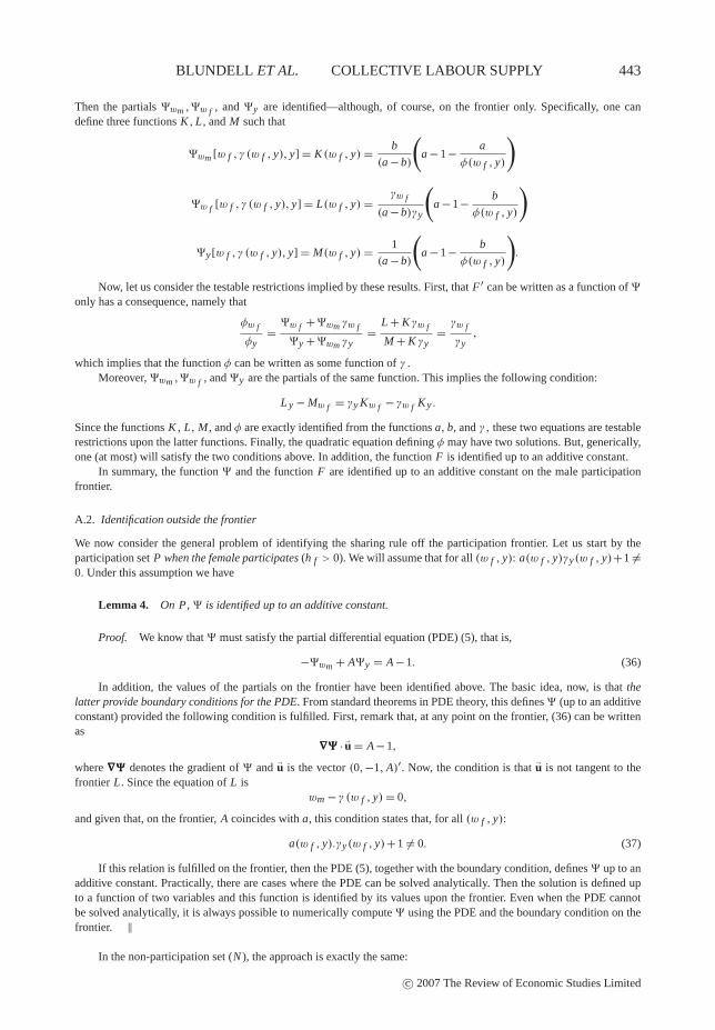
BLUNDELL ET AL. COLLECTIVE LABOUR SUPPLY 443
Then the partials �wm ,�w f , and �y are identified—although, of course, on the frontier only. Specifically, one candefine three functions K , L , and M such that
�wm [w f ,γ (w f , y), y] = K (w f , y) = b
(a −b)
(a −1− a
φ(w f , y)
)
�w f [w f ,γ (w f , y), y] = L(w f , y) = γw f
(a −b)γy
(a −1− b
φ(w f , y)
)
�y [w f ,γ (w f , y), y] = M(w f , y) = 1
(a −b)
(a −1− b
φ(w f , y)
).
Now, let us consider the testable restrictions implied by these results. First, that F ′ can be written as a function of �
only has a consequence, namely that
φw f
φy= �w f +�wm γw f
�y +�wm γy= L + Kγw f
M + Kγy= γw f
γy,
which implies that the function φ can be written as some function of γ .Moreover, �wm ,�w f , and �y are the partials of the same function. This implies the following condition:
L y − Mw f = γy Kw f −γw f Ky .
Since the functions K , L , M , and φ are exactly identified from the functions a, b, and γ, these two equations are testablerestrictions upon the latter functions. Finally, the quadratic equation defining φ may have two solutions. But, generically,one (at most) will satisfy the two conditions above. In addition, the function F is identified up to an additive constant.
In summary, the function � and the function F are identified up to an additive constant on the male participationfrontier.
A.2. Identification outside the frontier
We now consider the general problem of identifying the sharing rule off the participation frontier. Let us start by theparticipation set P when the female participates (h f > 0). We will assume that for all (w f , y): a(w f , y)γy(w f , y)+1 �=0. Under this assumption we have
Lemma 4. On P, � is identified up to an additive constant.
Proof. We know that � must satisfy the partial differential equation (PDE) (5), that is,
−�wm + A�y = A −1. (36)
In addition, the values of the partials on the frontier have been identified above. The basic idea, now, is that thelatter provide boundary conditions for the PDE. From standard theorems in PDE theory, this defines � (up to an additiveconstant) provided the following condition is fulfilled. First, remark that, at any point on the frontier, (36) can be writtenas
∇∇∇��� · u = A −1,
where ∇�∇�∇� denotes the gradient of � and u is the vector (0,−1, A)′. Now, the condition is that u is not tangent to thefrontier L . Since the equation of L is
wm −γ (w f , y) = 0,
and given that, on the frontier, A coincides with a, this condition states that, for all (w f , y):
a(w f , y).γy(w f , y)+1 �= 0. (37)
If this relation is fulfilled on the frontier, then the PDE (5), together with the boundary condition, defines � up to anadditive constant. Practically, there are cases where the PDE can be solved analytically. Then the solution is defined upto a function of two variables and this function is identified by its values upon the frontier. Even when the PDE cannotbe solved analytically, it is always possible to numerically compute � using the PDE and the boundary condition on thefrontier. ‖
In the non-participation set (N ), the approach is exactly the same:
c© 2007 The Review of Economic Studies Limited
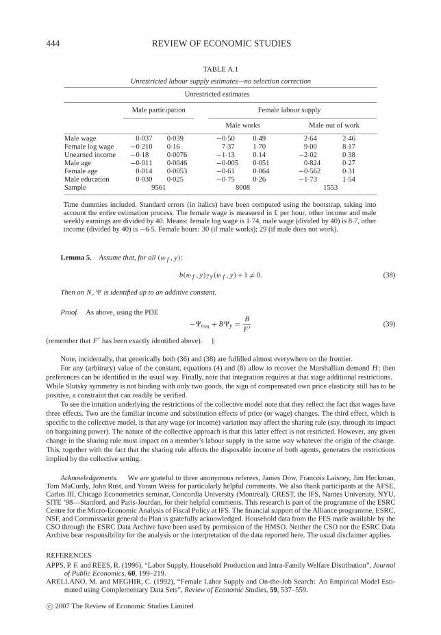
444 REVIEW OF ECONOMIC STUDIES
TABLE A.1
Unrestricted labour supply estimates—no selection correction
Unrestricted estimates
Male participation Female labour supply
Male works Male out of work
Male wage 0·037 0·039 −0·50 0·49 2·64 2·46Female log wage −0·210 0·16 7·37 1·70 9·00 8·17Unearned income −0·18 0·0076 −1·13 0·14 −2·02 0·38Male age −0·011 0·0046 −0·005 0·051 0·824 0·27Female age 0·014 0·0053 −0·61 0·064 −0·562 0·31Male education 0·030 0·025 −0·75 0·26 −1·73 1·54Sample 9561 8008 1553
Time dummies included. Standard errors (in italics) have been computed using the bootstrap, taking intoaccount the entire estimation process. The female wage is measured in £ per hour, other income and maleweekly earnings are divided by 40. Means: female log wage is 1·74, male wage (divided by 40) is 8·7, otherincome (divided by 40) is −6·5. Female hours: 30 (if male works); 29 (if male does not work).
Lemma 5. Assume that, for all (w f , y):
b(w f , y)γy(w f , y)+1 �= 0. (38)
Then on N, � is identified up to an additive constant.
Proof. As above, using the PDE
−�wm + B�y = B
F ′ (39)
(remember that F ′ has been exactly identified above). ‖
Note, incidentally, that generically both (36) and (38) are fulfilled almost everywhere on the frontier.For any (arbitrary) value of the constant, equations (4) and (8) allow to recover the Marshallian demand H ; then
preferences can be identified in the usual way. Finally, note that integration requires at that stage additional restrictions.While Slutsky symmetry is not binding with only two goods, the sign of compensated own price elasticity still has to bepositive, a constraint that can readily be verified.
To see the intuition underlying the restrictions of the collective model note that they reflect the fact that wages havethree effects. Two are the familiar income and substitution effects of price (or wage) changes. The third effect, which isspecific to the collective model, is that any wage (or income) variation may affect the sharing rule (say, through its impacton bargaining power). The nature of the collective approach is that this latter effect is not restricted. However, any givenchange in the sharing rule must impact on a member’s labour supply in the same way whatever the origin of the change.This, together with the fact that the sharing rule affects the disposable income of both agents, generates the restrictionsimplied by the collective setting.
Acknowledgements. We are grateful to three anonymous referees, James Dow, Francois Laisney, Jim Heckman,Tom MaCurdy, John Rust, and Yoram Weiss for particularly helpful comments. We also thank participants at the AFSE,Carlos III, Chicago Econometrics seminar, Concordia University (Montreal), CREST, the IFS, Nantes University, NYU,SITE ’98—Stanford, and Paris-Jourdan, for their helpful comments. This research is part of the programme of the ESRCCentre for the Micro-Economic Analysis of Fiscal Policy at IFS. The financial support of the Alliance programme, ESRC,NSF, and Commissariat general du Plan is gratefully acknowledged. Household data from the FES made available by theCSO through the ESRC Data Archive have been used by permission of the HMSO. Neither the CSO nor the ESRC DataArchive bear responsibility for the analysis or the interpretation of the data reported here. The usual disclaimer applies.
REFERENCESAPPS, P. F. and REES, R. (1996), “Labor Supply, Household Production and Intra-Family Welfare Distribution”, Journal
of Public Economics, 60, 199–219.ARELLANO, M. and MEGHIR, C. (1992), “Female Labor Supply and On-the-Job Search: An Empirical Model Esti-
mated using Complementary Data Sets”, Review of Economic Studies, 59, 537–559.
c© 2007 The Review of Economic Studies Limited
BLUNDELL ET AL. COLLECTIVE LABOUR SUPPLY 445
ATTANASIO, O. and MAZZOCCO, M. (2001), “Intra-Household Allocation with Limited Commitment: An EmpiricalCharacterization” (Mimeo, University of Wisconsin-Madison).
BLUNDELL, R., CHIAPPORI, P. A. and MEGHIR, C. (2005), “Collective Labour Supply with Children”, Journal ofPolitical Economy, 113, 1277–1306.
BLUNDELL, R. W., CHIAPPORI, P. A., MAGNAC, T. and MEGHIR, C. (2000), “Collective Labor Supply and House-hold Production” (Mimeo, University College London).
BLUNDELL, R. W., DUNCAN, A. and MEGHIR, C. (1998), “Estimating Labor Supply Using Tax Policy Reforms”,Econometrica, 66, 827–861.
BLUNDELL, R. W. and MACURDY, T. (1999), “Labor Supply: A Review of Alternative Approaches”, Handbook ofLabor Economics, 3, 1560–1695.
BLUNDELL, R. W. and WALKER, I. (1986), “A Life Cycle Consistent Empirical Model of Labor Supply Using CrossSection Data”, Review of Economic Studies, 53, 539–558.
BROWNING, M., BOURGUIGNON, F., CHIAPPORI, P.-A. and LECHENE, V. (1996), “Incomes and Outcomes: AStructural Model and Some Evidence from French Data”, Journal of Political Economy, 102, 1067–1096.
BROWNING, M. and CHIAPPORI, P.-A. (1998), “Efficient Intra-Household Allocations: A General Characterizationand Empirical Tests”, Econometrica, 66, 1241–1278.
CHIAPPORI, P.-A. (1988), “Rational Household Labor Supply”, Econometrica, 56, 63–89.CHIAPPORI, P.-A. (1992), “Collective Labor Supply and Welfare”, Journal of Political Economy, 100, 437–467.CHIAPPORI, P.-A. (1997), “Introducing Household Production in Collective Models of Labor Supply”, Journal of
Political Economy, 105, 191–209.CHIAPPORI, P.-A. and DONNI, O. (2005), “Learning From a Piece of Pie: The Empirical Content of Nash Bargaining”
(Mimeo, Columbia University).CHIAPPORI, P.-A. and EKELAND, I. (2002), “The Micro Economics of Group Behavior: Identification” (Mimeo,
University of Chicago).CHIAPPORI, P.-A. and EKELAND, I. (2006), “The Micro Economics of Group Behavior: General Characterization”,
Journal of Economic Theory, 130 (1), 1–26.CHIAPPORI, P.-A., FORTIN, B. and LACROIX, G. (2002), “Marriage Market, Divorce Legislation and Household
Labor Supply”, Journal of Political Economy, 110, 37–72.DONNI, O. (2003), “Collective Household Labor Supply: Nonparticipation and Income Taxation”, The Journal of Public
Economics, 87, 1179–1198.DONNI, O. (2004), “Labor Supply, Home Production and Welfare Comparisons” (Mimeo, University of Cergy-Pontoise).DUFLO, E. (2003), “Grandmothers and Granddaughters: Old Age Pension and Intra-Household Allocation in South
Africa”, World Bank Economic Review, 17, 1–25.FORTIN, B. and LACROIX, G. (1997), “A Test of Neoclassical and Collective Models of Household Labor Supply”,
Economic Journal, 107, 933–955.GOSLING, A., MACHIN, S. and MEGHIR, C. (2000), “The Changing Distribution of Male Wages in the UK”, Review
of Economic Studies, 67, 635–666.HADDAD, L. and KANBUR, R. (1992), “Intra-Household Inequality and the Theory of Targeting”, European Economic
Review, 36, 372–378.KAPTEYN, A. and KOOREMAN, P. (1992), “Household Labour Supply: What Kind of Data Can Tell Us How Many
Decision Makers There Are?”, European Economic Review, 36, 365–371.KOOREMAN, P. and KAPTEYN, A. (1990), “On the Implementation of Some Game Theoretic Models of Household
Labor Supply”, Journal of Human Resources, 25, 584–598.LIGON, E. (2002), “Dynamic Bargaining in Households” (Mimeo, University of California, Berkeley).LUNDBERG, S. (1988), “Labor Supply of Husbands and Wives”, Review of Economics and Statistics, 70, 224–235.MACLEOD, B. and MALCOMSON, J. (1993), “Investments, Holdup, and the Form of Market Contracts”, American
Economic Review, 83, 811–837.MACURDY, T. (1983), “A Simple Scheme for Estimating an Intertemporal Model of Labor Supply and Consumption in
the Presence of Taxes and Uncertainty”, International Economic Review, 24, 265–289.MAZZOCCO, M. (2003a), “Intertemporal Behavior and Household Structure” (Manuscript, Department of Economics,
University of Wisconsin-Madison).MAZZOCCO, M. (2003b), “Household Intertemporal Behavior: A Collective Characterization and a Test of Commit-
ment” (Manuscript, Department of Economics, University of Wisconsin-Madison).MAZZOCCO, M. (2004), “Savings, Risk Sharing and Preferences for Risk”, American Economic Review, 94, 1169–
1182.MEGHIR, C. and WHITEHOUSE, E. (1997), “Labour Market Transitions and Retirement in the UK”, Journal of Econo-
metrics, 79 (2), 327–354.NEARY, J. P. and ROBERTS, K. W. S. (1980), “The Theory of Household Behaviour under Rationing”, European
Economic Review, 13, 24–35.THOMAS, D. (1990), “Intra-Household Resource Allocation: An Inferential Approach”, Journal of Human Resources,
25, 635–664.UDRY, C. (1996), “Gender, Agricultural Production, and the Theory of Household”, Journal of Political Economy, 104
(5), 1010–1046.ZHANG, J. and FONG, K. (2001), “The Identification of Unobservable Independent and Spousal Leisure”, Journal of
Political Economy, 109, 191–202.
c© 2007 The Review of Economic Studies Limited