Collaborative co- clustering across multiple social...

Collaborative co-clustering across

multiple social mediaFengjiao Wang Shuyang Lin Philip S. Yu

Department of Computer Science, University of Illinois at Chicago

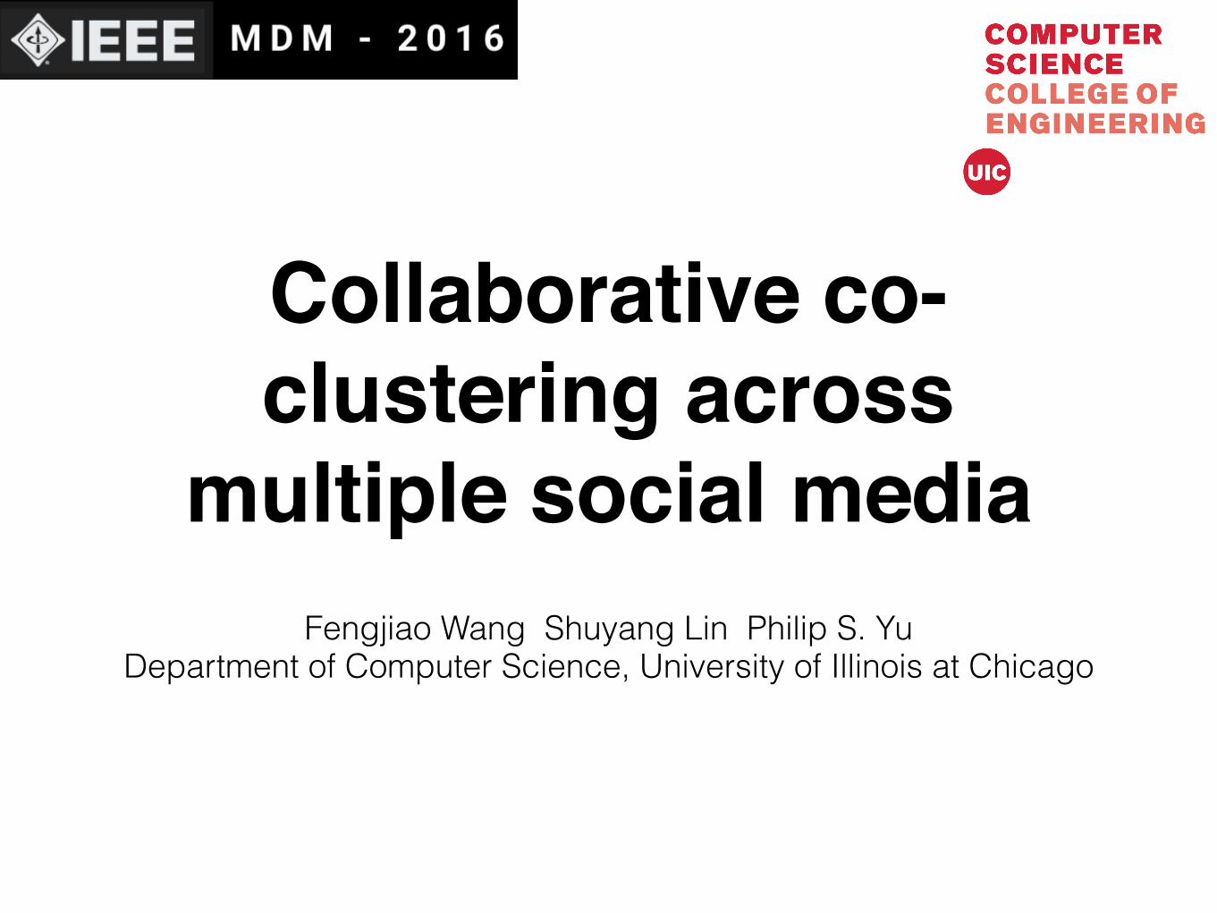
Location-based social networks

share location

review

find nearby friends

social

discover POI

Main activities in location-based social networks

“check-in”

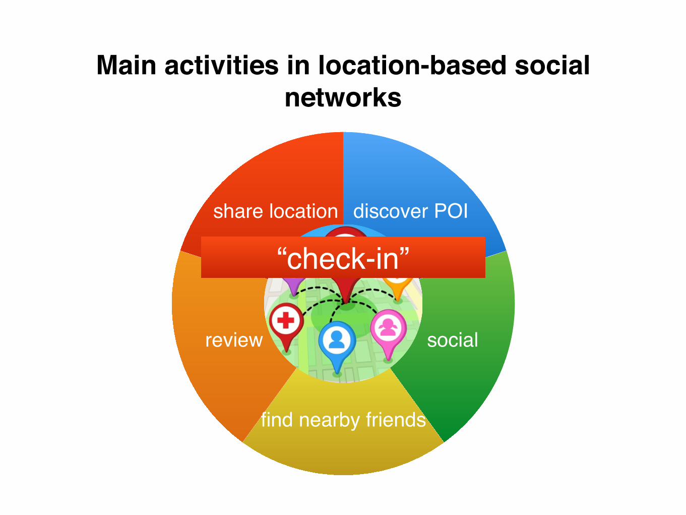
Aligned networks

same user

Twitter & Foursquare Kickstarter & Twitter

Twitter

Foursquare

Kickstarter

Twitter

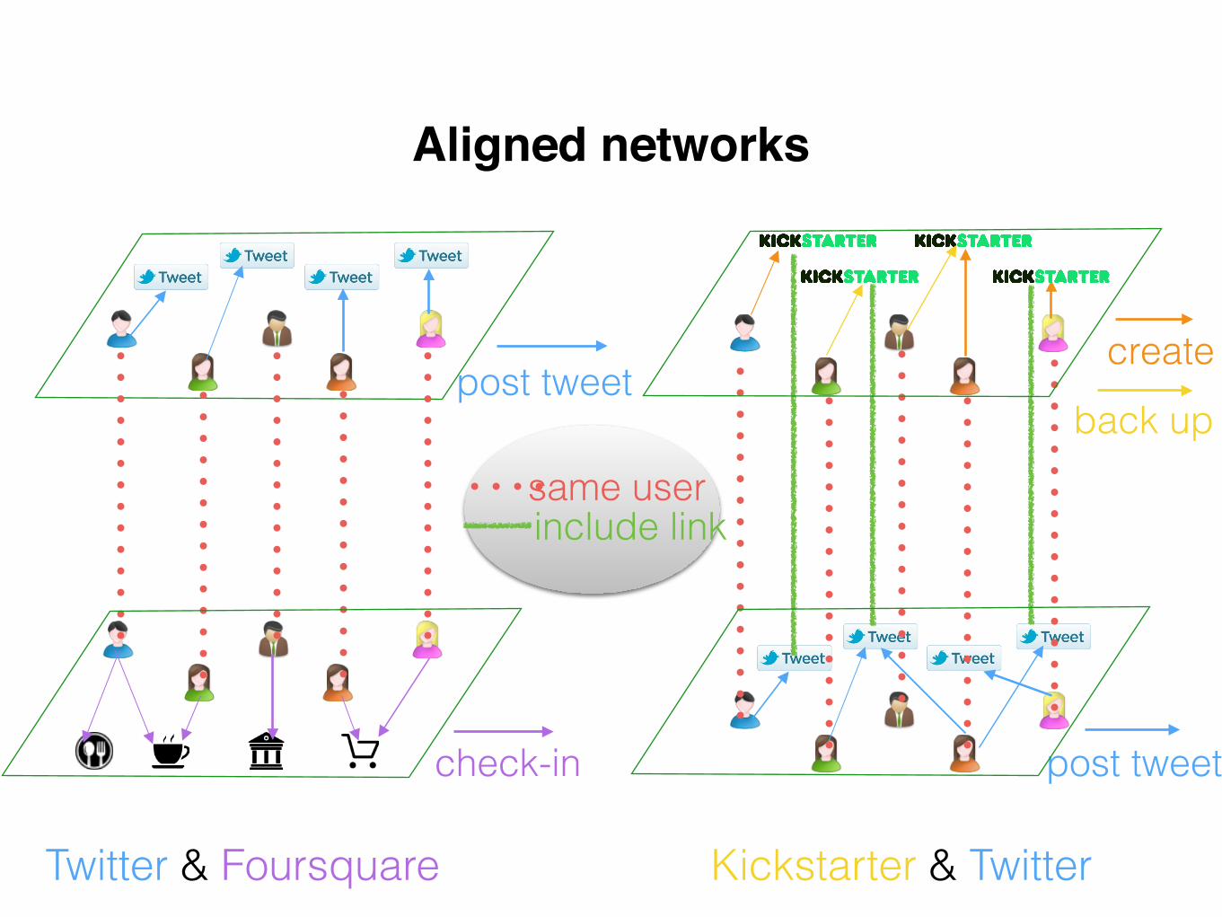
Aligned networks

post tweet

check-in post tweet

create

back upsame userinclude link

Twitter & Foursquare Kickstarter & Twitter

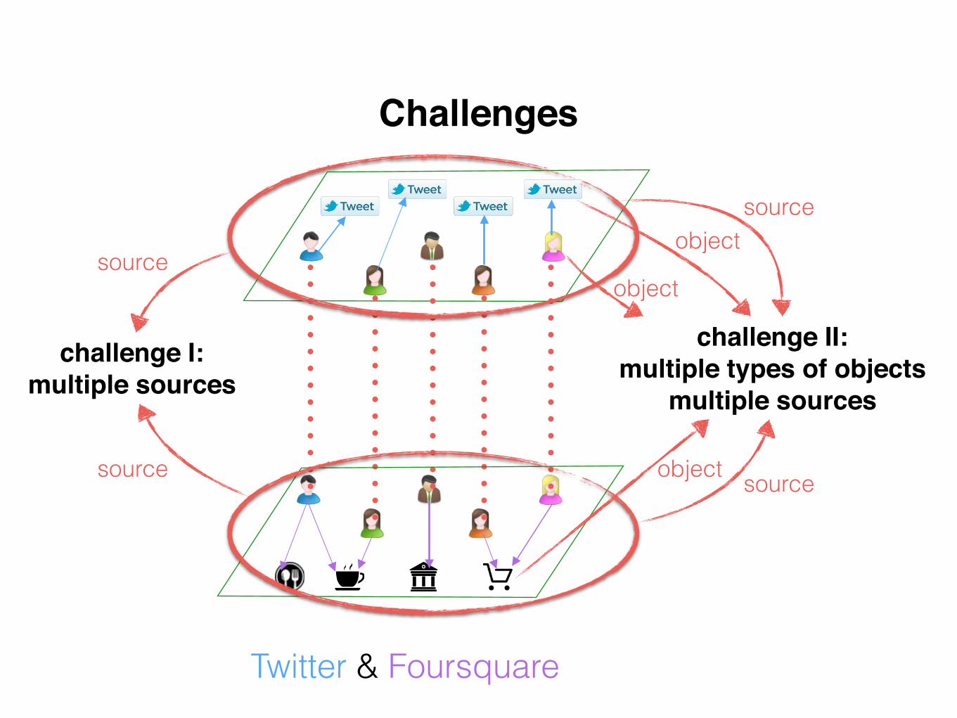
Challenges

Twitter & Foursquare

source

challenge I: multiple sources

challenge II: multiple types of objects

multiple sources

source

sourceobject

sourceobject

object

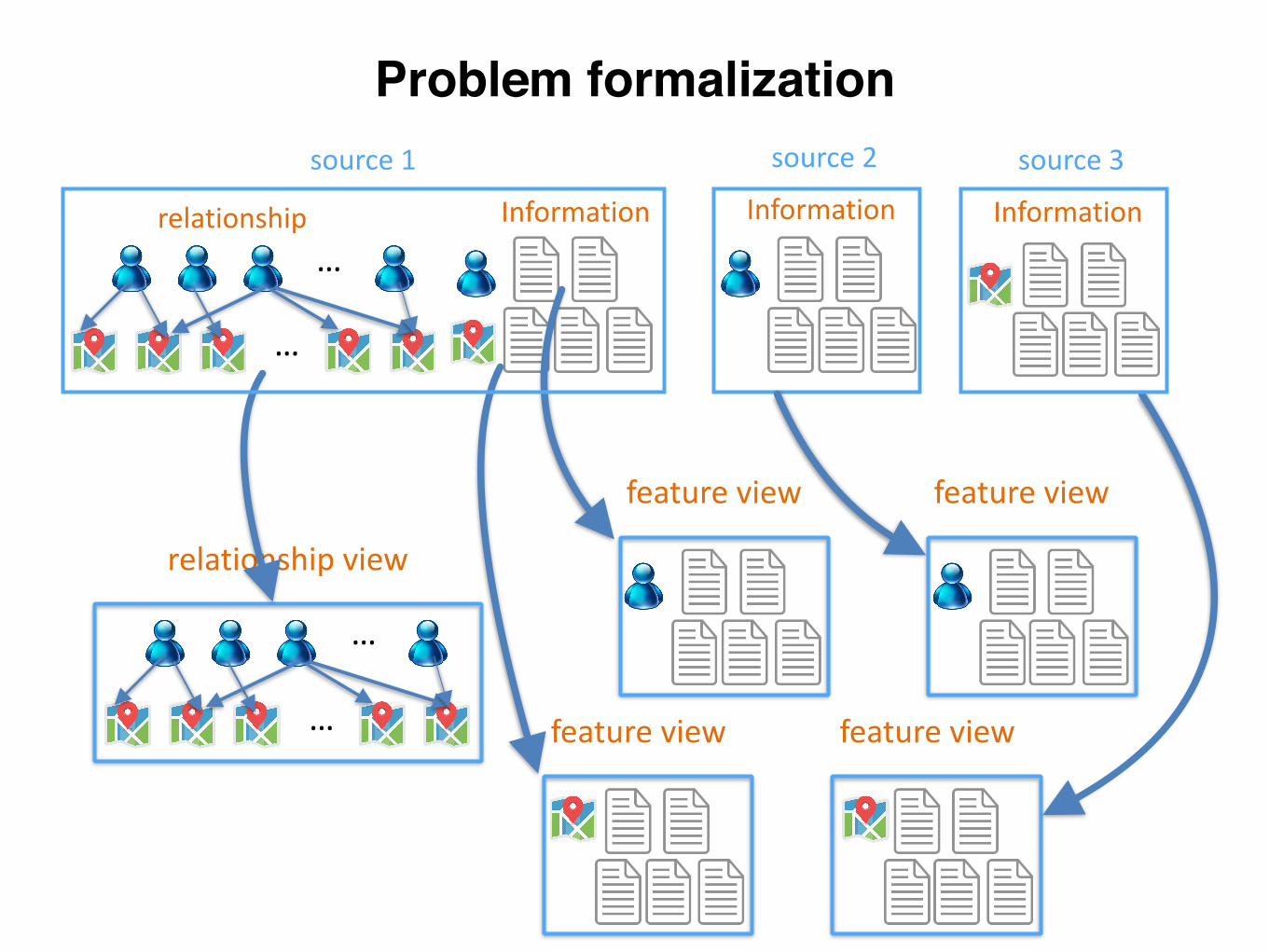
Problem formalization

relationship…

…

relationshipview

…

…

source1 source3

featureview featureview

featureview

Information Information

source2

featureview

Information

relationshipview

…

…

featureview featureview

Co-regularizedcollaborativeco-clustering

spectralclusteringspectralco-clustering

co-regularization

co-clustering

…

……

…clustering

……

……

clustering

……

…

…

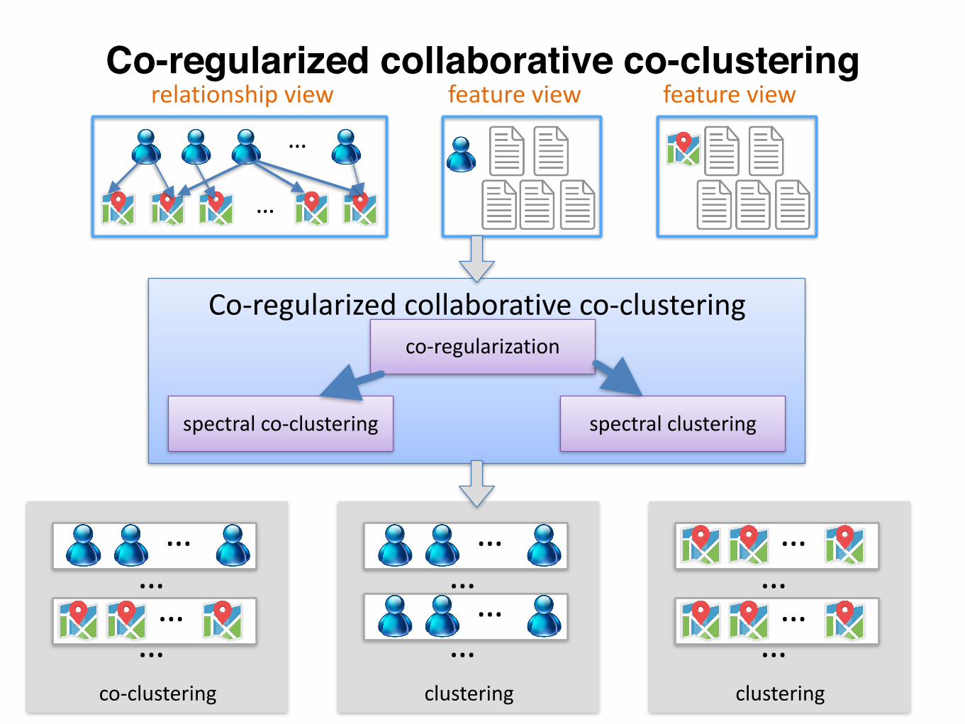
Co-regularized collaborative co-clustering

Objective function the other one into two feature matrices. We follow the no-tations of spectral co-clustering. Assume there are m objectA and n object B, the relationship matrix between objectA and object B is E. Feature matrices in feature views arecomputed using Gaussian kernel. We denote kernel matrixof object A in view w as K(w)

A . We also denote kernel matrix

of object B in view p as K(p)B . Our goal is to find co-cluster

result X, where X can be solved using E, K(w)A , and K

(p)B .

2.3 Co-regularized Collaborative Co-clusteringModel

In the proposed multi-view setting, objects are groupedinto co-cluster and clusters under di↵erent views. In orderto achieve better co-cluster by leveraging relationship view

and feature views, we can consider this problem as findingmaximum agreement between di↵erent views with regardsto the same types of objects. The dissimilarity between co-cluster and clusters are then measured by a co-regularizationterm, which is performed on the eigenvector matrices of co-cluster and clusters. The reasons why eigenvector matricesare utilized are listed below. First, Eigenvector matrices inspectral clustering/co-clustering represent the graph parti-tion rules, which is essentially the discriminative informationof clusters. Second, eigenvector matrix for two types of ob-jects in spectral co-clustering could be decomposed into twoeigenvector matrices corresponding to each type of objects.This would allow us to construct the co-regularization termfor each type of objects under di↵erent views.

Frobenius norm is employed to realize this co-regularization.Assume two eigenvector matrices are U(a) and U(b)), theFrobenius norm measures the distance between them, notedas D(U(a)

,U(b)), where

D(U(a),U(b)) = �Tr(U(a)U(a)TU(b)U(b)T )

Subsequently, maximizing agreement between two views isto minimize �Tr(U(a)U(a)TU(b)U(b)T ).

2.3.1 Co-regularized collaborative co-clusteringWe formulate the collaborative co-clustering problem as

an optimization problem which tries to find optimized graphpartitioning for spectral co-clustering and spectral cluster-ing in multiple views and maximize agreement between re-

lationship view and feature views. That being said, we willfirst perform spectral co-clustering on the relationship view,from which we can obtain a partition result represented asU(v). Also, spectral clustering will be performed on eachfeature view for A and B, where U

(w)A for 1 w W , and

U(p)B for 1 p P can be obtained. Then, U(v), U(w)

A ,

and U(p)B will be used as initial value for the optimization

algorithm. The objective function for optimization is shownin Equation 1. It is composed of three parts, i.e., the objec-tive function of co-clustering in relationship view, the objec-tive function in feature views, and objective function for theco-regularization. In particular, the first item is the spectralco-clustering objective function. The second and third itemsstand for the objective function under features views for Aand B, respectively. Note that multiple feature views existfor A and B, so they are both in a sum manner. As can beseen, the fourth and fifth items are in the shape of Frobe-nius norm, and therefore represent the objective functionfor co-regularization. It is worth to mention that since wecombine the objective function together as shown, it brings

us the merit of simultaneous clustering, co-clustering, andcollaboratively optimization.

minU(v),U

(w)A ,U

(p)B

tr(U(v)TL(v)U(v)) +X

1wW

tr(U(w)TA L

(w)A U

(w)A )

+X

1pP

tr(U(p)TB L

(p)B U

(p)B )

� �

X

1wW

tr(T1U(v)U(v)TT1

TU(w)A U

(w)TA )

� �

X

1pP

tr(T2U(v)U(v)TT2

TU(p)B U

(p)TB ) (1)

where U(w)TA U

(w)A = I, for 1 w W

U(p)TB U

(p)B = I, for 1 p P

L(v) =

"D

(v)r �E

�ET D(v)c

#

L(w)A = {D(w)

A }�1/2K(w)A {D(w)

A }�1/2, for 1 w W

L(p)B = {D(p)

B }�1/2K(p)B {D(p)

B }�1/2, for 1 p P

U(v) is eigenvector matrix in view v related to two typesof objects A and B. U

(w)A and U

(p)B are eigenvector matri-

ces in view w and view p related to object A and objectB respectively. L(v) is Laplacian matrix of co-clusteringin view v. L

(w)A and L

(p)B are Laplacian matrices of clus-

tering in view w and p. Matrices D(v)r , D

(v)c , D

(w)A , and

D(p)B are diagonal matrices, [D(v)

r ]ii =P

j Eij , [D(v)c ]ii =

Pj Eji, [D(w)

A ]i =P

j [K(w)A ]ij , and [D(p)

B ]i =P

j [K(p)B ]ij .

In co-regularization, to make eigenvector matrices U(v) andU

(w)A /U(p)

B compatible with each other, we define transitionmatrix T1 =

⇥Im⇥m 0m⇥n

⇤and T2 =

⇥0n⇥m In⇥n

⇤to

transfer U(v) to another matrix which only contain informa-tion in terms of the same type of objects with U

(w)A /U(p)

B .

Eigenvector matrix U(v) can be split into two matrices U(v)A

and U(v)B by equation U(v) =

"U

(v)A

U(v)B

#, where matrix U

(v)A

and U(v)B are eigenvector matrices corresponding to object

A and object B in view v respectively. Hyperparameter � isdefined to tradeo↵ original clusterings and co-regularizationterm.The proposed problem is a non-convex optimization prob-

lem since two non-convex terms for co-regularization are in-troduced in the objective function. We use alternating min-imization technique to solve this problem, since alternatingminimization provides a useful framework for iterative opti-mization in non-convex problem. In details, every eigenvec-tor matrix will be updated alternatively with other eigen-vector matrices being held fixed in each iteration. Since ananalytical solution can be found for each eigenvector matrixduring alternating minimization, repeating this process it-eratively will converge asymptotically in general. However,it is not the aim of this paper to prove this property. Wealso provide an intuitive interpretation of the proposed al-gorithm. Take object A as an example, the final clusters ofobject A should preserve original relationship with anothertype of object B and also be refined by clusters in otherviews. To avoid a clustering result that is either too closeto original co-cluster or too close to clusters in other views

the other one into two feature matrices. We follow the no-tations of spectral co-clustering. Assume there are m objectA and n object B, the relationship matrix between objectA and object B is E. Feature matrices in feature views arecomputed using Gaussian kernel. We denote kernel matrixof object A in view w as K(w)

A . We also denote kernel matrix

of object B in view p as K(p)B . Our goal is to find co-cluster

result X, where X can be solved using E, K(w)A , and K

(p)B .

2.3 Co-regularized Collaborative Co-clusteringModel

In the proposed multi-view setting, objects are groupedinto co-cluster and clusters under di↵erent views. In orderto achieve better co-cluster by leveraging relationship view

and feature views, we can consider this problem as findingmaximum agreement between di↵erent views with regardsto the same types of objects. The dissimilarity between co-cluster and clusters are then measured by a co-regularizationterm, which is performed on the eigenvector matrices of co-cluster and clusters. The reasons why eigenvector matricesare utilized are listed below. First, Eigenvector matrices inspectral clustering/co-clustering represent the graph parti-tion rules, which is essentially the discriminative informationof clusters. Second, eigenvector matrix for two types of ob-jects in spectral co-clustering could be decomposed into twoeigenvector matrices corresponding to each type of objects.This would allow us to construct the co-regularization termfor each type of objects under di↵erent views.

Frobenius norm is employed to realize this co-regularization.Assume two eigenvector matrices are U(a) and U(b)), theFrobenius norm measures the distance between them, notedas D(U(a)

,U(b)), where

D(U(a),U(b)) = �Tr(U(a)U(a)TU(b)U(b)T )

Subsequently, maximizing agreement between two views isto minimize �Tr(U(a)U(a)TU(b)U(b)T ).

2.3.1 Co-regularized collaborative co-clusteringWe formulate the collaborative co-clustering problem as

an optimization problem which tries to find optimized graphpartitioning for spectral co-clustering and spectral cluster-ing in multiple views and maximize agreement between re-

lationship view and feature views. That being said, we willfirst perform spectral co-clustering on the relationship view,from which we can obtain a partition result represented asU(v). Also, spectral clustering will be performed on eachfeature view for A and B, where U

(w)A for 1 w W , and

U(p)B for 1 p P can be obtained. Then, U(v), U(w)

A ,

and U(p)B will be used as initial value for the optimization

algorithm. The objective function for optimization is shownin Equation 1. It is composed of three parts, i.e., the objec-tive function of co-clustering in relationship view, the objec-tive function in feature views, and objective function for theco-regularization. In particular, the first item is the spectralco-clustering objective function. The second and third itemsstand for the objective function under features views for Aand B, respectively. Note that multiple feature views existfor A and B, so they are both in a sum manner. As can beseen, the fourth and fifth items are in the shape of Frobe-nius norm, and therefore represent the objective functionfor co-regularization. It is worth to mention that since wecombine the objective function together as shown, it brings

us the merit of simultaneous clustering, co-clustering, andcollaboratively optimization.

minU(v),U

(w)A ,U

(p)B

tr(U(v)TL(v)U(v)) +X

1wW

tr(U(w)TA L

(w)A U

(w)A )

+X

1pP

tr(U(p)TB L

(p)B U

(p)B )

� �

X

1wW

tr(T1U(v)U(v)TT1

TU(w)A U

(w)TA )

� �

X

1pP

tr(T2U(v)U(v)TT2

TU(p)B U

(p)TB ) (1)

where U(w)TA U

(w)A = I, for 1 w W

U(p)TB U

(p)B = I, for 1 p P

L(v) =

"D

(v)r �E

�ET D(v)c

#

L(w)A = {D(w)

A }�1/2K(w)A {D(w)

A }�1/2, for 1 w W

L(p)B = {D(p)

B }�1/2K(p)B {D(p)

B }�1/2, for 1 p P

U(v) is eigenvector matrix in view v related to two typesof objects A and B. U

(w)A and U

(p)B are eigenvector matri-

ces in view w and view p related to object A and objectB respectively. L(v) is Laplacian matrix of co-clusteringin view v. L

(w)A and L

(p)B are Laplacian matrices of clus-

tering in view w and p. Matrices D(v)r , D

(v)c , D

(w)A , and

D(p)B are diagonal matrices, [D(v)

r ]ii =P

j Eij , [D(v)c ]ii =

Pj Eji, [D(w)

A ]i =P

j [K(w)A ]ij , and [D(p)

B ]i =P

j [K(p)B ]ij .

In co-regularization, to make eigenvector matrices U(v) andU

(w)A /U(p)

B compatible with each other, we define transitionmatrix T1 =

⇥Im⇥m 0m⇥n

⇤and T2 =

⇥0n⇥m In⇥n

⇤to

transfer U(v) to another matrix which only contain informa-tion in terms of the same type of objects with U

(w)A /U(p)

B .

Eigenvector matrix U(v) can be split into two matrices U(v)A

and U(v)B by equation U(v) =

"U

(v)A

U(v)B

#, where matrix U

(v)A

and U(v)B are eigenvector matrices corresponding to object

A and object B in view v respectively. Hyperparameter � isdefined to tradeo↵ original clusterings and co-regularizationterm.The proposed problem is a non-convex optimization prob-

lem since two non-convex terms for co-regularization are in-troduced in the objective function. We use alternating min-imization technique to solve this problem, since alternatingminimization provides a useful framework for iterative opti-mization in non-convex problem. In details, every eigenvec-tor matrix will be updated alternatively with other eigen-vector matrices being held fixed in each iteration. Since ananalytical solution can be found for each eigenvector matrixduring alternating minimization, repeating this process it-eratively will converge asymptotically in general. However,it is not the aim of this paper to prove this property. Wealso provide an intuitive interpretation of the proposed al-gorithm. Take object A as an example, the final clusters ofobject A should preserve original relationship with anothertype of object B and also be refined by clusters in otherviews. To avoid a clustering result that is either too closeto original co-cluster or too close to clusters in other views

co-clustering

clustering

co-regulariza/on

Experiment setup: dataset

• ReutersMulAlingualdataset

• 1200documents,6categorieswithregardstotopics.DocumentswriGenin5differentlanguagescorrespondingto5views.

• WebKBdataset(Cornell,Texas,Washington,Wisconsin)

• 4sub-datasetsofwebpagesextractedfromcomputersciencedepartmentof4universiAes:Cornell,Texas,Washing,andWisconsin.Webpagesareclassifiedinto5categories(student,project,course,staff,faculty).

• Foursquare+TwiGerdataset

• 881Foursquareuserswhocheckedin10,285Amesat780venues.

Reuters dataset

0"

0.2"

0.4"

0.6"

0.8"

1"

1.2"

KL_doc" KL_word" KL_total"

CoClust"

ITCC"

MssrIcc"

MssrIIcc"

Co:CoClust"

(a) KL divergence

0"

0.1"

0.2"

0.3"

0.4"

0.5"

15" 20" 25" 30"cluster(number(

CoClust"ITCC"MssrIcc"MssrIIcc"Semi"Best_view"Feature_concat"Mul?@view_pair"Mul?@view_centroid"Co@CoClust"

(b) NMI

0.64%

0.66%

0.68%

0.7%

0.72%

0.74%

0.76%

15% 20% 25% 30%cluster(number(

CoClust%ITCC%MssrIcc%MssrIIcc%Semi%Best_view%Feature_concat%MulBCview_pair%MulBCview_centroid%CoCCoClust%

(c) RI

0"

0.05"

0.1"

0.15"

0.2"

0.25"


CoClust"ITCC"MssrIcc"MssrIIcc"Semi"Best_view"Feature_concat"Mul>?view_pair"Mul>?view_centroid"Co?CoClust"

(d) Accuracy

Figure 2: Reuters Dataset

0"

0.2"

0.4"

0.6"

0.8"

1"


CoClust"

ITCC"

MssrIcc"

MssrIIcc"

Co:CoClust"

(a) KL divergence

0"

0.1"

0.2"

0.3"

0.4"

0.5"


CoClust"ITCC"MssrIcc"MssrIIcc"Semi"Best_view"Feature_concat"Mul@Aview_pair"Mul@Aview_centroid"CoACoClust"

(b) NMI

0"0.1"0.2"0.3"0.4"0.5"0.6"0.7"0.8"


CoClust"ITCC"MssrIcc"MssrIIcc"Semi"Best_view"Feature_concat"MulBCview_pair"MulBCview_centroid"CoCCoClust"

(c) RI

0"0.1"0.2"0.3"0.4"0.5"0.6"0.7"0.8"


CoClust"

ITCC"

MssrIcc"

MssrIIcc"

Semi"

Best_view"

Feature_concat"

MulBCview_pair"

MulBCview_centroid"

(d) Accuracy

Figure 3: Cornell Dataset

Cornell dataset

0"

0.2"

0.4"

0.6"

0.8"

1"

1.2"


CoClust"

ITCC"

MssrIcc"

MssrIIcc"

Co:CoClust"

(a) KL divergence

0"

0.1"

0.2"

0.3"

0.4"

0.5"


CoClust"ITCC"MssrIcc"MssrIIcc"Semi"Best_view"Feature_concat"Mul?@view_pair"Mul?@view_centroid"Co@CoClust"

(b) NMI

0.64%

0.66%

0.68%

0.7%

0.72%

0.74%

0.76%

15% 20% 25% 30%cluster(number(

CoClust%ITCC%MssrIcc%MssrIIcc%Semi%Best_view%Feature_concat%MulBCview_pair%MulBCview_centroid%CoCCoClust%

(c) RI

0"

0.05"

0.1"

0.15"

0.2"

0.25"


CoClust"ITCC"MssrIcc"MssrIIcc"Semi"Best_view"Feature_concat"Mul>?view_pair"Mul>?view_centroid"Co?CoClust"

(d) Accuracy

Figure 2: Reuters Dataset

0"

0.2"

0.4"

0.6"

0.8"

1"


CoClust"

ITCC"

MssrIcc"

MssrIIcc"

Co:CoClust"

(a) KL divergence

0"

0.1"

0.2"

0.3"

0.4"

0.5"



(b) NMI

0"0.1"0.2"0.3"0.4"0.5"0.6"0.7"0.8"



(c) RI

0"0.1"0.2"0.3"0.4"0.5"0.6"0.7"0.8"


CoClust"

ITCC"

MssrIcc"

MssrIIcc"

Semi"

Best_view"

Feature_concat"

MulBCview_pair"

MulBCview_centroid"

(d) Accuracy

Figure 3: Cornell Dataset

Texas dataset

0"0.2"0.4"0.6"0.8"1"

1.2"1.4"


CoClust"

ITCC"

MssrIcc"

MssrIIcc"

Co:CoClust"

(a) KL divergence

0"0.05"0.1"0.15"0.2"0.25"0.3"0.35"0.4"



(b) NMI

0"0.1"0.2"0.3"0.4"0.5"0.6"0.7"0.8"



(c) RI

0"0.1"0.2"0.3"0.4"0.5"0.6"0.7"0.8"



(d) Accuracy

Figure 4: Texas Dataset

0"

0.5"

1"

1.5"

2"


CoClust"

ITCC"

MssrIcc"

MssrIIcc"

Co8CoClust"

(a) KL divergence

0"0.05"0.1"0.15"0.2"0.25"0.3"0.35"0.4"


CoClust"ITCC"MssrIcc"MssrIIcc"Semi"Best_view"Feature_concat"MulABview_pair"MulABview_centroid"CoBCoClust"

(b) NMI

0"0.1"0.2"0.3"0.4"0.5"0.6"0.7"0.8"



(c) RI

0"0.1"0.2"0.3"0.4"0.5"0.6"0.7"



(d) Accuracy

Figure 5: Washington Dataset

Washington dataset

0"0.2"0.4"0.6"0.8"1"

1.2"1.4"


CoClust"

ITCC"

MssrIcc"

MssrIIcc"

Co:CoClust"

(a) KL divergence

0"0.05"0.1"0.15"0.2"0.25"0.3"0.35"0.4"



(b) NMI

0"0.1"0.2"0.3"0.4"0.5"0.6"0.7"0.8"



(c) RI

0"0.1"0.2"0.3"0.4"0.5"0.6"0.7"0.8"



(d) Accuracy

Figure 4: Texas Dataset

0"

0.5"

1"

1.5"

2"


CoClust"

ITCC"

MssrIcc"

MssrIIcc"

Co8CoClust"

(a) KL divergence

0"0.05"0.1"0.15"0.2"0.25"0.3"0.35"0.4"



(b) NMI

0"0.1"0.2"0.3"0.4"0.5"0.6"0.7"0.8"



(c) RI

0"0.1"0.2"0.3"0.4"0.5"0.6"0.7"



(d) Accuracy

Figure 5: Washington Dataset

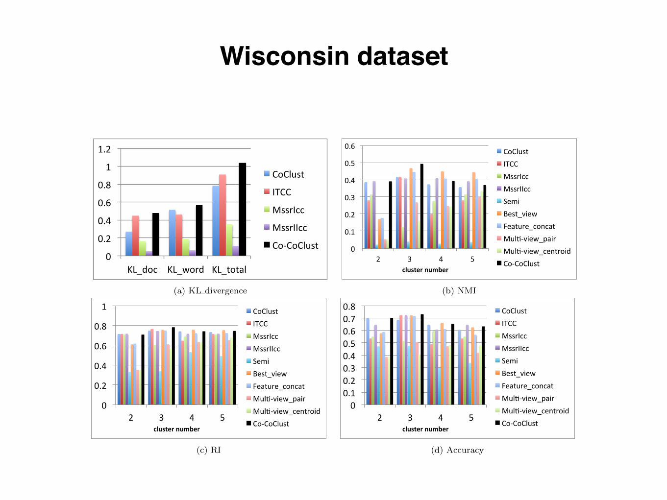
Wisconsin dataset

0"

0.2"

0.4"

0.6"

0.8"

1"

1.2"


CoClust"

ITCC"

MssrIcc"

MssrIIcc"

Co:CoClust"

(a) KL divergence

0"

0.1"

0.2"

0.3"

0.4"

0.5"

0.6"



(b) NMI

0"

0.2"

0.4"

0.6"

0.8"

1"



(c) RI

0"0.1"0.2"0.3"0.4"0.5"0.6"0.7"0.8"



(d) Accuracy

Figure 6: Wisconsin Dataset

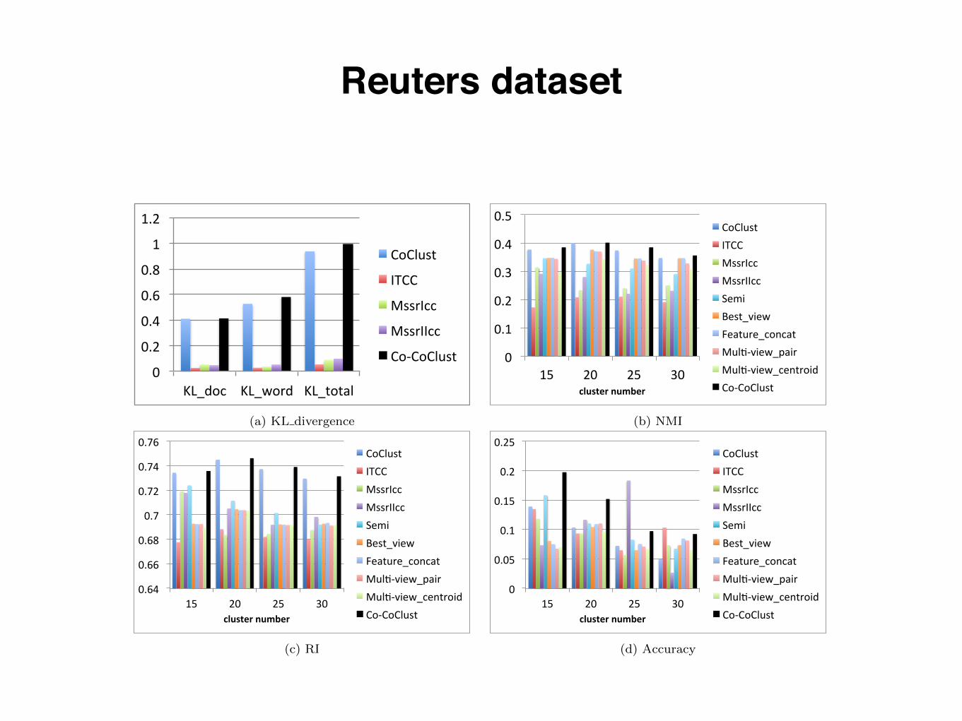
over the best of the baselines. Figure 2(c) gives RI re-sults, where Co-CoClust shows the best performance onall four cases. Co-CoClust achieves good overall Accu-racy. Especially, when cluster number equals to 15 and 20,Co-CoClust achieves 28% improvement over best of base-lines. When number of clusters equals to 25, Co-CoClustobtains second best results.

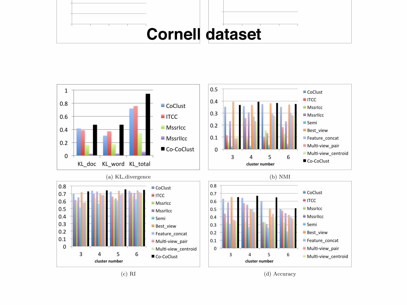
Evaluation results on Cornell dataset is shown in Fig-ure 3. Figure 3(a) shows KL divergence of document andword clusters, where Co-CoClust achieves much better re-sults compared with other baselines. Quality of documentclusters is being evaluated by other metrics with varyingnumber of clusters from 3 to 6, as shown in Figure 3(b)-(d).Co-CoClust achieves the best results on 3 cases and onesecond best result when number of clusters equals to 3 inFigure 3(b) . In Figure 3(c) and Figure 3(d), Co-CoClustachieve the best results on RI and Accuracy.

Figure 4 demonstrates evaluation results onTexas dataset.Again, the proposed approach performs well on KL divergencemetric in Figure 4(a). We can also observe from Figure 4(b),Figure 4(c), and Figure 4(d) that Co-CoClust consistentlyachieves better results. For instance, in Figure 4(d), Co-CoClust improves second best method by 10% averagingover di↵erent cluster number.

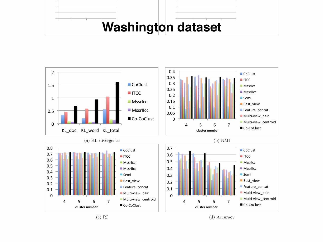
Evaluation results onWashington dataset is summarizedin Figure 5. Co-CoClust achieves consistently better re-sults than baselines by a significant margin on KL divergence.In the evaluation of NMI, RI, and Accuracy, Co-CoClustperforms better than co-clustering based methods and multi-view based methods in most of cases.

Figure 6 illustrates performance of the proposed approachand 9 baselines on Wisconsin dataset. Co-CoClust ob-tains the best results in KL divergence in Figure 6(a). Co-CoClust also achieves better results on NMI, RI, and Ac-

curacy overall compared with baseline algorithms.To sum up, the proposed Co-CoClust performs consis-

tently better than single view clustering, co-clustering, andmulti-view clustering algorithms on both social networksand document-word datasets. It proves that the proposedmodel steadily outperforms most of the state of the art al-gorithms in combining multiple source information for co-clustering problems.

3.2.2 Social network datasetThis dataset severs as a case study for a practical ap-

plication in social network. Unlike Reuters and webKBdatasets which have ground truth, social network datasetdid not provide any ground truth for user clusters or clus-ters of social media objects. Moreover, it is hard to manuallylabel users or social media objects with high quality. There-fore, in this paper, we employ a di↵erent evaluation strategyto show the performance of the proposed Co-CoClust onsocial network dataset. The idea is to justify the e�cacyand robustness of the proposed approach on utilizing par-tially observed information for the task of clustering place.With an increasing percentage of random information loss,we want to evaluate how the proposed algorithm performsto deal with the information loss by means of compensatingthe loss via multi-sources learning. Figure 7 shows compar-ison results when the percentage of information loss rangesfrom 10% to 60%. The “ground truth” is produced by k-means algorithm on full information in terms of place. Fig-ure 7(a) depicts NMI of the proposed approach and base-lines. In general, all of the other algorithms su↵ers moredegradation when more information being hidden from ex-periment. However, Co-CoClust consistently performs thebest in the perspectives of NMI and Accuracy as shown inFigure 7(a) and Figure 7(c), which demonstrates the ro-

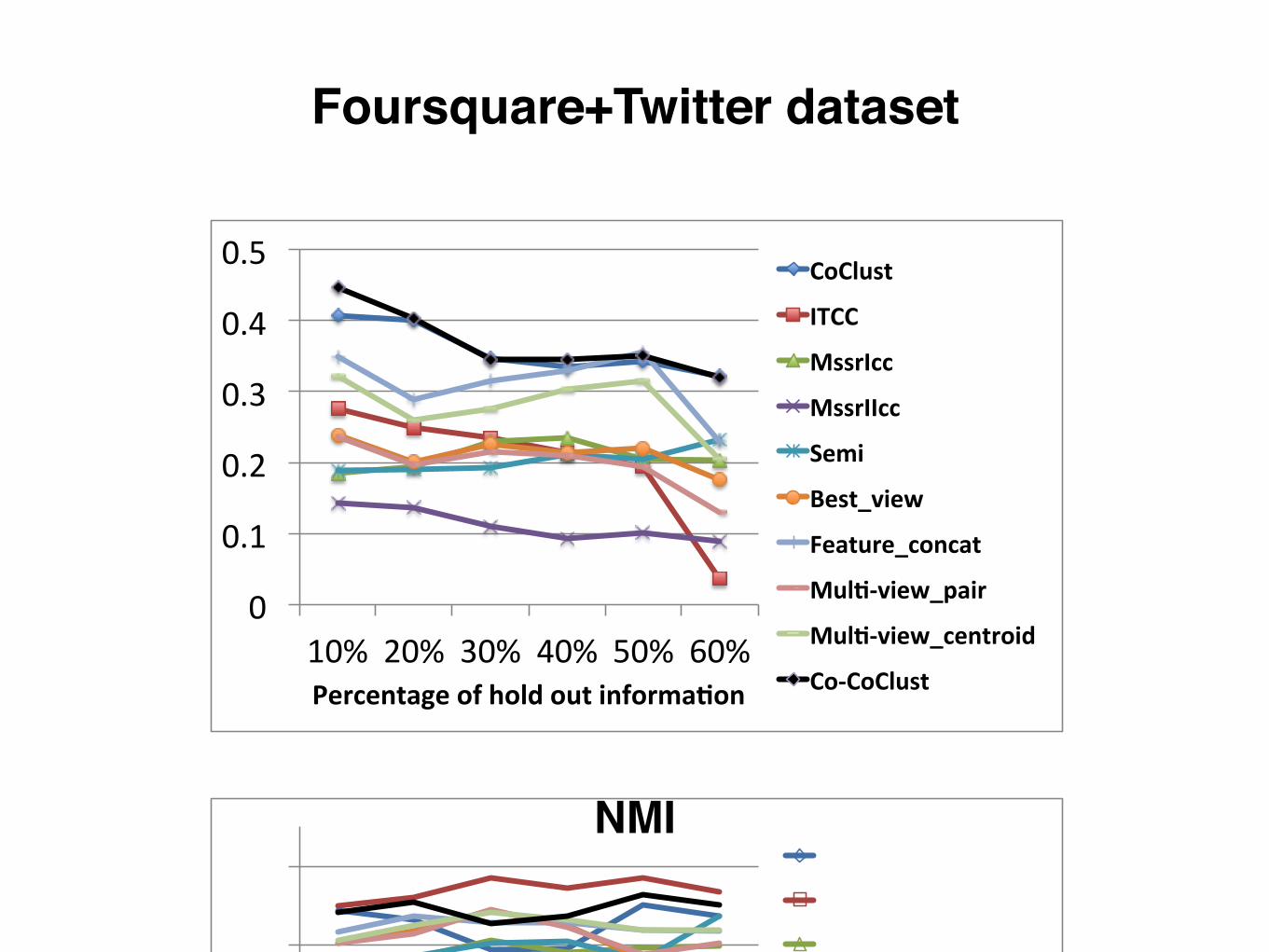
Foursquare+Twitter dataset

0"

0.1"

0.2"

0.3"

0.4"

0.5"

10%" 20%" 30%" 40%" 50%" 60%"Percentage)of)hold)out)informa2on)

CoClust)

ITCC)

MssrIcc)

MssrIIcc)

Semi)

Best_view)

Feature_concat)

Mul2>view_pair)

Mul2>view_centroid)

Co>CoClust)

(a) NMI

0"

0.2"

0.4"

0.6"

0.8"


CoClust)

ITCC)

MssrIcc)

MssrIIcc)

Semi)

Best_view)

Feature_concat)

Mul2>view_pair)

Mul2>view_centroid)

Co>CoClust)

(b) RI

0"0.1"0.2"0.3"0.4"0.5"0.6"0.7"


CoClust)

ITCC)

MssrIcc)

MssrIIcc)

Semi)

Best_view)

Feature_concat)

Mul2>view_pair)

Mul2>view_centroid)

Co>CoClust)

(c) Accuracy

Figure 7: Foursquare+Twitter

bustness of Co-CoClust. Co-CoClust obtains the secondbest results when evaluated by RI as shown in Figure 7(b).Overall, Co-CoCluster outperforms other algorithms in com-bining multi-source information for co-clustering problems.

4. RELATED WORKCo-clustering algorithm earns a lot of attentions from re-

search communities in data mining and machine learningdue to its capability to cluster two types of objects or ob-ject and feature simultaneously [9, 10, 16]. Co-clusteringalgorithms also prove to be a powerful data mining tech-nique on practical applications such as text mining, socialrecommendation, mining networks. Spectral co-clusteringalgorithm proposed by Dhillon et al. ([9]) utilizes graphpartitioning technique for the co-clustering of the bipartitegraph of documents and words. It attracts a lot of attentionssince the objective function is well formulated and could besolved as a eigenvector problem. Other co-clustering algo-rithms are also proposed to embrace di↵erent technique onsimultaneously clustering two types of objects ([10]). Re-

cently, researchers have developed many new co-clusteringalgorithms to add constraints ([16, 18]) or side information([15, 20, 22]). [16] integrates additional information as con-straints into a semi-supervised co-clustering algorithm. [18]proposed information theoretic co-clustering framework fortext mining. In [15], the authors claim that using metadataas constraint in co-clustering achieves better performancethan metadata-driven and metadata-injected. [12] works onco-clustering multiple domains of objects, achieving clus-terings of multiple types of objects by linear combination.However, researches on developing a reasonable yet flexiblemethod to handle additional information other than usingthem as constraints are limited.The rise of multi-representation data create an opportu-

nity for multi-view learning. Many multi-view based cluster-ing algorithms ([3, 5, 11, 13, 14]) have also been proposed.[3] describes an extension of the classical k-means algorithmand EM algorithm for multi-view setting. [5] uses CanonicalCorrelation Analysis to extract relevant features from mul-tiple views, and then apply classical clustering algorithm.Non-negative matrix factorization technique is also exploitedin multi-view setting ([11, 14]). [14] assumes that not all ex-amples are presented in all views and propose a non-negativematrix factorization based model for clustering under par-tially observed data. Multi-view clustering also sees its ap-plication in web 2.0 items ([13]). Similar with this paperwhich utilize social media objects in multi-view clustering,we did co-clustering on social media objects.Recently, several algorithms in multi-view setting are pro-

posed for spectral clustering ([1, 2, 8, 19, 21, 23]). [23]generalizes single view normalized cut approach to multipleviews to obtain a graph cut by random walk based formula-tion. In [8], the authors focus on two view case of multi-viewclustering by creating a bipartite graph. Spectral clusteringis applied on the constructed bipartite graph. Instead ofworking on original features, [1] takes di↵erent clusteringscoming from di↵erent sources as input and reconcile themto find a final clustering. It is suggested that they couldachieve better performance by directly working on cluster-ings instead of original features of multiple source informa-tion. Another paper [2] also works on clusterings instead oforiginal features. They employ co-regularization techniqueto force clusterings learned from di↵erent views of the dataagree with each other. Working on clusterings instead oforiginal features shows good performance on clustering onetype of objects. Inspired by the success in clustering, in thispaper, we are working on co-clustering two types of objectson multiple source information.Other multi-view clustering algorithms ([6, 17]) also uti-

lize co-regularization technique. [17] implements multi-viewregularization of unlabeled examples to perform semi-supervisedlearning. [4] works on clustering multiple types of objectswith their relationship matrices. Relationship matrices areutilized to compute co-similarity matrices. Then, di↵erentco-similarity matrix with respect to the same type of ob-jects are combined for generating clustering result. Thereare two major di↵erences between [4] and our work. First ofall, they transfer co-clustering problem of multiple types ofobjects into clustering problems via co-similarity matrices.However, in this paper we proposed a direct co-clusteringframework to simultaneously clustering multiple types of ob-jects in the original space. Secondly, paper [4] implementsthe idea of combining multiple source information by com-

NMI

• ObservaAons

• DatasparsenessonLBSN.

• Co-clusteringusersandplacescouldbenefitlocaAonrecommendaAon.

• Idea

• CastproblemoflearninguserandplacepaGernsfrommulAplesources(alignedFoursquareandTwiGernetworks)asmulA-viewlearningproblem.

• Co-regularizingclustersofthesametypeofobjectsacrossdifferentsourcestolearnco-clusterintargetsource.

• UAlizespectralco-clusteringandspectralclusteringtolearnco-cluster(targetsource)andclusters(othersources)simultaneously.

Conclusion

Q & A?

[email protected]

mailto:[email protected]

Collaborative co- clustering across multiple social...

Documents

Transcript of Collaborative co- clustering across multiple social...