
COKPUTATION OF CANONICAL CORREZATION BEST … · COKPUTATION OF CANONICAL CORREZATION AND BEST...
18
COKPUTATION OF CANONICAL CORREZATION AND BEST PREDICTABLE ASPECT OF FUTURE FOR TIHE SERIES Mohsen Pourahmadil University of California, Davisz A.G. Miamee3 Hampton University Hampton, Virginia ABSTRACT: The canonical correlation between the (infinite) past and future of a stationary time series is shown to be the limit of the canonical correlation between the (infinite) past and (finite) future, and computation of the latter is reduced to a (generalized) eigenvalue problem involving (finite) matrices. This provides a convenient and, essentially, finite- dimensional algorithm for computing canonical correlations and components of a time series. An upper bound is conjectured for the largest canonical correlation. (NASA-CR-184t55) COBFUTATICL OF CALIJOLSZCAL N89-14810 CCBBELATION ANC EEST PBEDICTAELk A5PECT UP PCTUXE FOR TIRE SEBXBS (California Uoiv-) I& P CSCL 128 Unclas 63/65 0185084 'Research supported by the NSF grant DMS-8601858. 20n leave from Northern Illinois Universit9.- 3Research supported in part by the NASA Grant NAG-1-768. https://ntrs.nasa.gov/search.jsp?R=19890005439 2018-07-17T02:44:13+00:00Z
Transcript of COKPUTATION OF CANONICAL CORREZATION BEST … · COKPUTATION OF CANONICAL CORREZATION AND BEST...

COKPUTATION OF CANONICAL CORREZATION AND BEST PREDICTABLE ASPECT OF FUTURE FOR TIHE SERIES
Mohsen Pourahmadil University of California, Davisz
A.G. Miamee3 Hampton University Hampton, Virginia
ABSTRACT: The canonical correlation between the (infinite) past and future
of a stationary time series is shown to be the limit of the canonical
correlation between the (infinite) past and (finite) future, and
computation of the latter is reduced to a (generalized) eigenvalue problem
involving (finite) matrices. This provides a convenient and, essentially,
finite- dimensional algorithm for computing canonical correlations and
components of a time series. An upper bound is conjectured for the
largest canonical correlation.
(NASA-CR-184t55) COBFUTATICL OF CALIJOLSZCAL N89-14810 C C B B E L A T I O N ANC EEST PBEDICTAELk A5PECT UP P C T U X E FOR T I R E SEBXBS ( C a l i f o r n i a U o i v - ) I & P CSCL 128 Unclas
63/65 0185084
'Research supported by the NSF grant DMS-8601858.
20n leave from Northern Illinois Universit9.-
3Research supported in part by the NASA Grant NAG-1-768.
https://ntrs.nasa.gov/search.jsp?R=19890005439 2018-07-17T02:44:13+00:00Z

1. Introduction
For many practical and theoretical problems in time series analysis,
cf. Akaike (1975), Tsay and Tiao (1985), Pourahmadi (1985), it is of
interest to know or compute p the canonical or maximal correlation
be tween the past
P - [ . . . I Xt+Xtl',
F - [Xt+l,Xt+2, * * 1 '
and the future
of a stationary time series CXt3, and the corresponding canonical
component or the best predictable aspect of future. Using the familiar
ideas from multivariate analysis, this task, requires computation of
eigenvalues, eigenvectors and inversion of infinite matrices or
operators.
For ARMA processes canonical correlations and components can be
computed (exactly) by solving linear systems of algebraic equations, cf.
Helson and Szeg6 (1960) and Yaglom (1983). For general stationary
processes, Jewel1 et. al. (1983) have given an algorithm for
computing (approximathg) the canonical correlations as the eigenvalues
of an infinite-dimensional (Hankel) operator, in the spectral domain.
In this paper, we provide a time domain algorithm for computing
(approximating) canonical correlations of a (nondeterministic)
stationary process, which requires only solving linear system(s) of
algebraic equations, cf. Yaglom (1965). For instance, in our approach,
computation of pm, the canonical correlation between the (infinite) past
P and (finite) future
ir-
Fm [xt+l, - - . ( ~ t + m ~ ' ,
requires solving one (generalized) eigenvalue problem for two mxm

2
matrices Gm and rm, cf. Theorem 2.3. Our approach relies primarily on the Wold ucomposition of a
(nondeterministic) stationary process; this makes it possible to reduce
the genuinely infinite-dimensional problem of computation of pm or p to
an, essentially, finite-dimensional problem; in addition to its
computational simplicity, this approach also provides a procedure for
computing p even when it does not exist as an eigenvalue of an operator,
cf. Jewell and Bloomfield (1983) and Jewell et. al. (1983).
In section 2 , we develop a procedure for computing the best
predictable aspect of (finite) future; the main result is Theorem 2.3.
This result along with a simple fact about geometry of Hilbert spaces are
used in Section 3 , to give an algorithm for computing p and the best
predictable aspect of the entire future. This procedure is applied to
the well-known models fitted to the sunspot numbers series; it turns out
that even for m-4, Pm provides a good approximation for p .
An interesting and yet open problem in this area is that of finding
is an upper a sharp upper bound for p ; we have conjectured that
bound for p , where u ' ~ is the interpolation error of a missing value
based on the other values of the process. Throughout th i s paper, we have
emphasized computation of the largest canonical correlation; other
canonical correlations and components can be computed by following a
standard procedure in multivariate analysis, c*f. Theorem 2.3.
0 ' 2 11-
2. Best Predictable Aspect of (Finite) Future
For many practical and theoretical problems it is of interest to
find the best predictable aspect of the future of a system; when the
system is modelled by a stochastic process CXtl, the problem of interest
3
. 4
can be r e s t a t e d a s t h a t of f ind ing the b e s t p red ic tab le l i n e a r func t iona l
of the fu tu re va lues of the form
where IDSOD and c 1 , . . . , cm a r e (necessar i ly) unknown; when m - m, ( 2 . 1 )
should be viewed as the l i m i t i n the mean of f i n i t e l i n e a r combination s.r<
I n genera l , t h i s is a hard problem t o solve.
c -
For t h e t i m e being, w e dea l with the simpler problem of f ind ing the
b e s t l i n e a r p red ic to r and p red ic t ion e r r o r of X i n (2 .1) when m and
c 1 , . . e , c, a r e known, and then i n the next s e c t i o n w e show how the
s o l u t i o n of t h i s apparent ly simpler problem can be employed t o resolve
the more d i f f i c u l t problem of f ind ing the b e s t p red ic t ab le aspec t of the
f u t u r e . The need f o r p red ic i ton of l i n e a r func t iona ls of t he form (2.1),
with known m and c l , . . . , cm, a r i s e s when the fo recas t e r is i n t e r e s t e d not
only i n a f o r e c a s t of ind iv idua l fu tu re values bu t a l s o i n fo recas t of a
l i n e a r combination of m f u t u r e values and a confidence i n t e r v a l f o r i t .
For example, i f s a l e s a r e recorded monthly, t he fo recas t e r might be
in te res ted i n the f o r e c a s t of next year ' s t o t a l sales ( m - 12, c1 - . . . I c12 - l ) , o r one might be i n t e r e s t e d i n fo recas t ing the average of some
f u t u r e va lues (c1 - .. . - cm - l/m), etc.
Note t h a t when c1 - . . . - C m - 1 - 0 and Cm - 1, then X - Xt+,,,, and
the p red ic t ion problem of X t + m can be solved i n the t i m e domain by using
the Wold decomposition of CXtl; i n f a c t , with
*-
m m

,
representing the Wold decomposition of CXtl, where Cctl is the
innovation process of CXtl and CVtl a deterministric process uncorrelated
with Cctl, the best linear predictor of Xt+r is given by
A aD
xt+r kzr bkc t+r-k + Vt+r
and its (mean square) prediction error is
( 2 . 3 )
Note that ( 2 . 2 ) also gives rise to the following representation of
r (7i-jlilj-l,a' the covariance matrix of CXtl:
where T = [bj-i]i,j-lla with bj - 0 for j < 0 , and I'v is the covariance
matrix of the deterministic process cVt3. As it is expected, the
prediction problem of the more general linear functional (2.1) also
hinges on the Wold decomposition of CXtl. Indeed, from (2.1) and ( 2 . 2 )
we have a m m k-0 r-1 r-1 x c ( c Crbr+k-mICt+m-k + C Vt+r,
m-1 m m (k-O k-m r-1 r-1
+ c ] ( c Crbr+k-m]ct+m-k + CrVt+r,
A
from t h i s , X the best linear predictor of X based on P is

5
n
Consider t h e harmonizable process {X t 8 R) c Lo(P) 2 given by Xt =l eiteZ(d8) t s
and i ts spectral bimeasure which is induced by Z , i . e eS .- -
F(A,B)'= E Z(A) z(B).
2 W e claim t h a t t h e corresponding s p e c t r a l domain L (P) i n t h i s case is notcomplete.
Ver i f ica t ion . By our..Eemma t h e r e exists a nonzero vector i n H (--)'which does Y
not have a series representa t ion as i n (4). Take one such vec tor V, Since V
is
combination of Y 's; k < 0 which converges t o V i n L (P).
n c l e a r l y i n H (0) t he re exists a sequence C ak Y-k =V of f i n i t e linear Y n 2 0
We can write - k
a
where t h e nonzero funct ions f n a By our Theorem i n sec t ion 2 w e have k'
are defined on pos i t i ve in t ege r s with f "(k) = n n
I I f n - f m II, = I I vn - vmI1
Now s i n c e v converges t o v and hence is Cauchy so is f However t h i s
p a r t i c u l a r sequence f
f i n L (P). Because otherwise another appl ica t ion of theTheorem i n sec t ion
2 shows t h a t f is i n L (Z) and
n n' 2 of func t ions i n L (F) does not converge t o any element n
2
1
Thus ye see t h a t V a l s o converges t o fdz , So I, m n f dZ == f ( i ) 2 ({i)) - E f ( i ) X i YmiS
i=o i=o
which con t r ad ic t s our choice ofV,
REMARK 1. Our example shows t h a t the main r e s u l t of C71 claiming t h e i -
completeness of t he spectral domain of any mul t iva r i a t e weakly harmonizable
process X is f a l s e even f o r a un iva r i a t e s t rongly harmonizable' process, t
. 2. We f e e l t h a t t h e e r r o r i n C73 occurs i n l i n e s 8 and 9 of t he
second column of page 4612 , where the ex is tence of a "ce r t a in pro jec t ion onto
a subspace" is asse r t ed and a re ference t o page 33 bf [ 9 3 is.made t o -
.
support i t . I n view of t he r e s u l t s es tab l i shed i n t h i s note t h e r e s u l t s i n

6
which is a quadratic form whose matrix is the matrix of prediction
errors. For computational purposes, it is important to note that the
matrix G, is, indeed, the upper left mxm submatrix of the matrix
G - u2T'T, (2.8)
where the (infinite) matrix T is as in (2.5), this provides a simple
method of computing Gm when the moving average parameters bl,b2, . . . are known or the task of Cholesky factorization of the covariance matrix I'
is accomplished. In the following rm also stands for the upper left mxm submatrix of r .
The measure of (linear) predictability of any function X is usually
defined as
cf. Jewel1 and Bloomfield (1983).
Next, we summarize some of the previous results.
Lemma 2.1. Let EXt} be a nondeterministic stationary process with
covariance function En3 and moving average parameters bo - 1,
bl,b2,. . . ,X - C crXt+r where m < QD and c1, ..., cm are given real
constants. Then, with X denoting the best linear predictor of X based
m
r-1 A
on the infinite past Xt,Xt-l, . . . , w e have
(a) Var(X-X) - C'Gmc. A
(b) the measure of (linear) predictability of X is given by c'Gm c C'rm c * *. X(X) - 1 -
Remark 2.2. For m-1, the measure of predictability of X - Xt+l has the simple form X(Xt+l) - 1 - u2/-yo, cf. Lemma 2.l(b), since u2 - expCJlog f(X) dX/27r}, where f(X) is the spectral density of the process,
it follows that X(Xt+l) can be expressed in terms of the density of the
process. However, for e l , it seems difficult to find expressions for
X(X) in terms of the density.
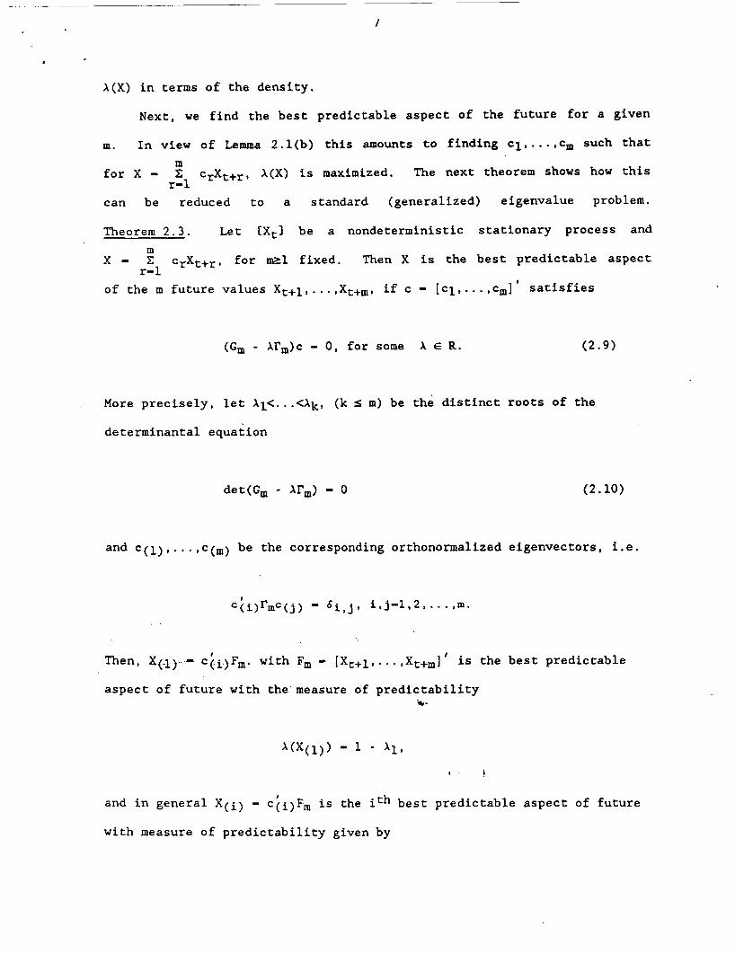
Next, we find the best predictable aspect of the future for a given
m. In view of Lemma 2.l(b) this amounts to finding c1,. . . ,cm such that for X - C crXt+r, X(X) is maximized. The next theorem shows how this
can be reduced to a standard (generalized) eigenvalue problem.
m
r-l
Theorem 2 . 3 . Let EXt) be a nondeterministic stationary process and
X - C c ~ X ~ + ~ , for e l fixed. Then X is the best predictable aspect
of the m future values Xt+l, . . . , Xt+,, if c - [c1 , . . . , cm]' satisfies m
r-1
(G, - Um)c - 0, for some X E R. (2 .9 )
More precisely, let X i < . . .<Xk, (k I m) be the distinct roots of the
determinantal equation
det(Gm - XI',) - 0 (2.10)
and ~(11, ..., c(~) be the corresponding orthonormalized eigenvectors, i.e.
cii>r,c(j) - 6 i , j . i S . j - 1 , 2 * - - ,m.
Then, Xf-l)-- cii.)Fm. with Fm - [Xt+l,. . . ,Xt+m] ' is the best predictable aspect of future with the'measure of predictability
h-
and in general X(i) - cti)Fm is the ith best predictable aspect of future with measure of predictability given by
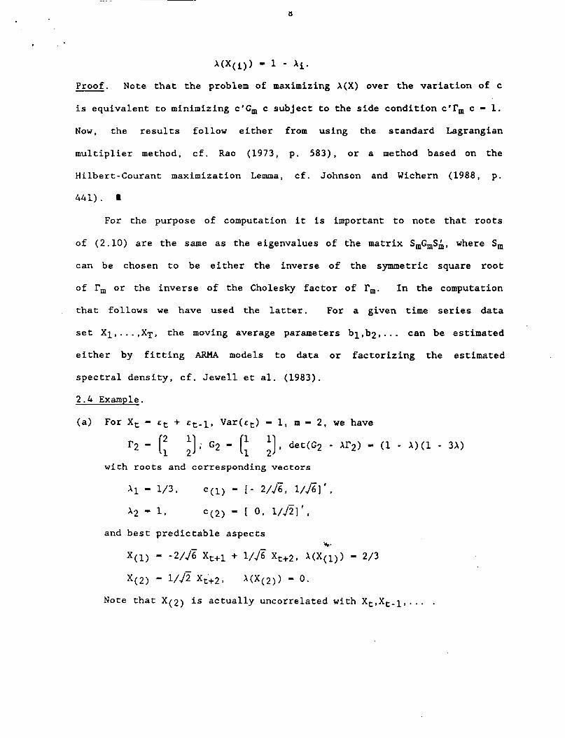
UX(i)> - 1 - Xi. Proof. Note that the problem of maximizing X(X) over the variation of c
is equivalent to minimizing c'Gm c subject to the side condition C'rm c - 1. Now, the results follow either from using the standard Lagrangian
multiplier method, cf. Rao (1973, p. 583), or a method based on the
Hilbert-Courant maximization Lemma, cf. Johnson and Wichern (1988, p.
441) . I
For the purpose of computation it is important to note that roots
of (2.10) are the same as the eigenvalues of the matrix SmGmSh, where Sm
can be chosen to be either the inverse of the symmetric square root
of rm or the inverse of the Cholesky factor of rm. In the computation
that follows we have used the latter, For a given time series data
set XI, . . . , XT, the moving average parameters bl,b2, ... can be estimated either by fitting ARMA models to data or factorizing the estimated
spectral density, cf. Jewel1 et al. (1983).
with roots and corresponding vectors
Note that X(2) is actually uncorrelated with Xc,Xt-l, . . . .
9
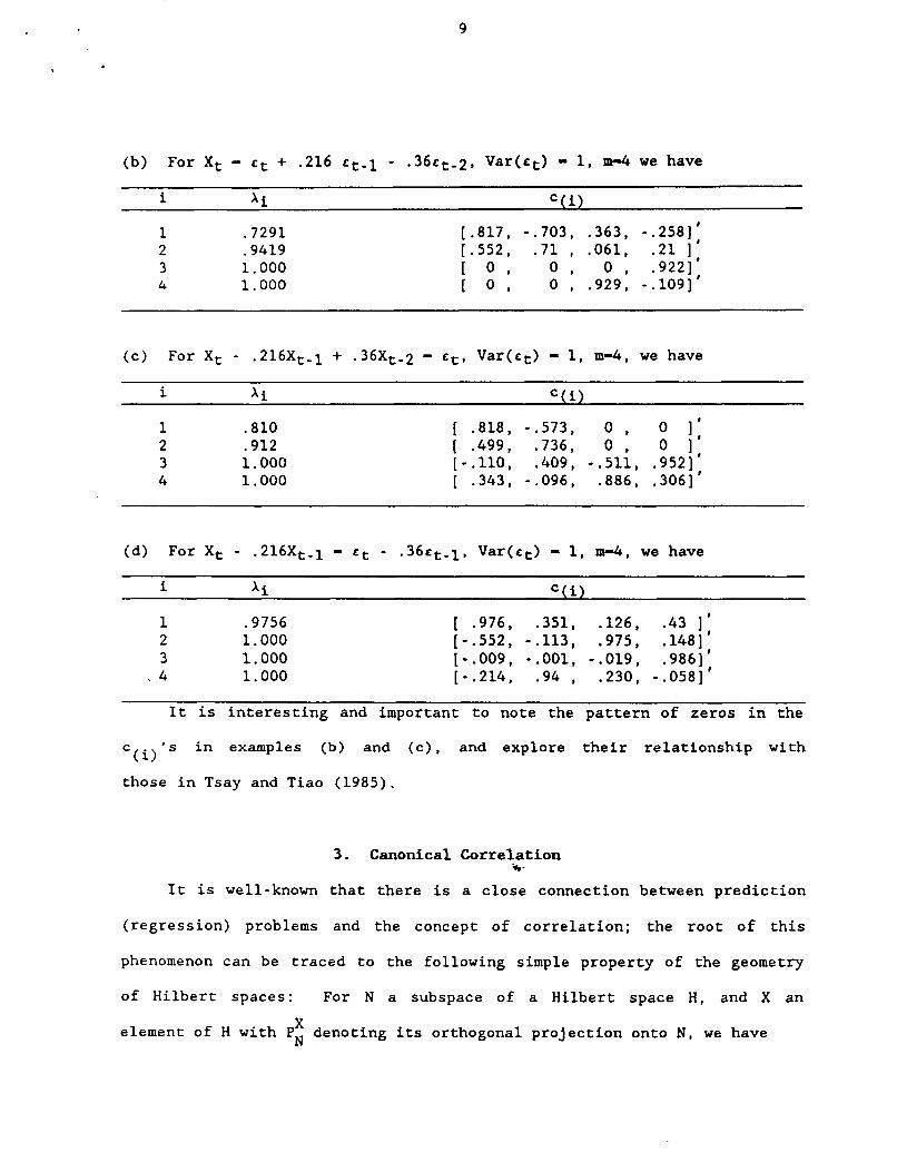
i xi C ( i )
1 2 3 4
.7291
.9419 1.000 1.000
[.817, -.703, ,363, -.258]) [.552, .71 , ,061, .21 1 ) [ 0 , 0 , 0 , .9221D
0 8 0 , ,929, -.109]'
( c ) For Xt - .216Xt-1 + .36Xt,2 - tt, Var(ct) - 1, m-4, we have i xi C( i)
.810
.912 1.000 1 * 000
[ .818, -.573, 0 , 0 1; [ .499, .736, 0 , 0 1, [-.110, ,409, -.511, .952] [ .343, -.096, .886, .306]'
(d) For Xt - .216Xt,1 - tt - .36ct,l, Var(ct) - 1, m-4, we have
i xi C(i)
1 2 3 4
.9756 1.000 1.000 1.000
[ .976, .351, .126, .43 1 ' [-.552, -.113, ,975, .148]' [-.009, -.001, -.019, .986]' [-.214, .94 , .230, -.058]'
It is interesting and important to note the pattern of zeros in the
c 's in examples (b) and (c), and explore their relationship with
those in Tsay and Tiao (1985). (i)
3. Canonical Correlation *- It is well-known that there is a close connection between prediction
(regression) problems and the concept of correlation; the root of this
phenomenon can be traced to the following simple property of the geometry
of Hilbert spaces: For N a subspace of a Hilbert space H, and X an
element of H with P X N denoting its orthogonal projection onto N, we have
10
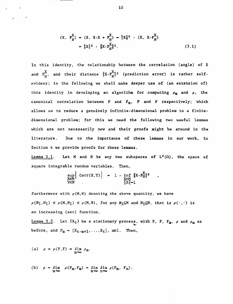
In this identity, the relationship between the correlation (angle) of X
X X and PN, and their distance lIX-PNI12 (prediction error) is rather self-
evident; in the following we shall make deeper use of (an extension of)
this identity in developing an algorithm for computing pm and p , the
canonical correlation between P and Fm, P and F respectively; which
allows us to reduce a genuinely infinite-dimensional problem to a finite-
dimensional problem; for this we need the following two useful lemmas
which are not necessarily new and their proofs might be around in the
literature. Due to the importance of these lemmas in our work, in
Section 4 we provide proofs for these lemmas.
Lemma 3.1. Let M and N be any two subspaces of L2(n>, the space of
square integrable random variables. Then,
furthermore with p(M,N) denoting the above quantity, we have
p(M1,Nl) I p(M,N1) I p(M,N), for any MiGI4 and N i a , that is p ( - ; ) is
an increasing (set) function.
Lemma 3 . 2 . Let CXtl be a stationary process, with P, F, Fm, p and pm as
before, and Pm - [Xt-m+l,...,Xt], e l . Then, i -
(b) p = Jim p(Pm,Fm) - Jim Jim p(P,, Fn). m- m* n+=
11
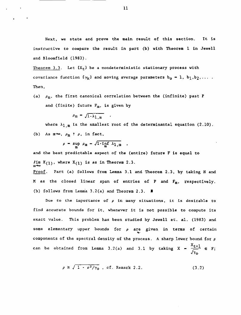
Next, we state and prove the main result of this section. It is
instructive to compare the result in part (b) with Theorem 1 in Jewell
and Bloomfield (1983).
Theorem 3 . 3 . Let CX,l be a nondeterministic stationary process with
covariance function Cykl and moving average parameters bo = 1, b11b2, . . . . Then,
(a) p m , the first canonical correlation between the (infinite) past P
and (finite) future Fm, is given by
where Xl,m is the smallest root of the determinantal equation (2.10).
(b) As m-, pm t p , in fact,
P S:P P m A-iqf Xl,m ,
and the best predictable aspect of the (entire) future F is equal to
lim X ( 1 ) , where X(1) is as in Theorem 2.3. m+- Proof. Part (a) follows from Lemma 3.1 and Theorem 2.3, by taking N and
M as the closed linear span of entries of P and Fm, respectively.
(b) follows from Lemm'a 3.2(a) and Theorem 2.3. I
Due to the importance of p in many situations, it is desirable to
find accurate bounds for it, whenever it is not possible to compute its
exact value. This problem has been studied by Jewell et. al. (1983) and
some elementary upper bounds for p are given in terms of certain
components of the spectral density of the process. A sharp lower bound for p
E F; can be obtained from Lemma 3.2(a) and 3.1 by taking X - - *-
Xt+l JG
P 2 J 1 - 02/70 , cf. Remark 2.2. (3.2)

12
. To show that this bound is sharp, note that for an AR(1) process
Xt - aXt,l + ct, u2 = 1, lalcl, 1 - we have yo - 1 - a 2 and the bound J 1 - a2/-yo - la1 is attained by p . It
is much harder to find a sharp upper bound for p ; however, motivated by
(3.2) we conjecture that when p < l , then
where u t 2 is the interpolation error of Xt+l based on CX,; s + t+l3.
We note that the bound ( 3 . 3 ) is attained for the aforementioned
AR(1) process, since in this case, by using a result of Kolmogorov (1941),
we have
u I 2 - (s f-'(8)dd/2r)'l - 1,
where f(B) - 11 - aeis1-2 is the spectral density of the AR(1) process,
A more solid motivation for the bound in ( 3 . 3 ) is the fact that p ( . , - ) ,
cf. Lemmas 3.1 and 3.2, is an increasing (set) function of its arguments;
- therefore, replacing N ( P ) by N1 - spCX,; s z t+l3, one arrives at a bound
of the form
J 1 - K ~ ' ~ / r ~ , %-
for p , where K is a constant. Thus, the conjecture amounts to showing
that K - 1. Remark 3 . 4 . The canonical correlation between P and F(k) - (Xt+k,
Xt+k+l,. . . f, krl fixed, denoted by p(k) , can be also computed by the
procedure developed in this paper. In fact, for any m > k, and taking c -

13
(0, . . . , O,ck+l, . . . , cm] one can prove results similar to those in Sections 2 and 3 for pm-k(k), which is the largest correlation between P and
[Xk+l, . . . , X,]. It is evident that Pm-k(k) -B p(k) as m -D -, cf. Theorem
the smallest root of
det(GA.k - X m - k ] - 0 ,
where GA,k is the (m-k)x(m-k) matrix obtained from Gm by deleting its
first k rows and k columns.
Example 3.5. The well-known sunspot numbers series has been studied by
many people and various models fitted to the data are given in Table 1,
cf. Jewell et al. (1983). We have calculated p 4 , that is the canonical
correlation between P and F4, and the corresponding canonical component,
using the method of Theorem 3.3, see Table 2. These results are very
close to the results in Table 2 of Jewell et al. (1983) which contains the
value p for these models; this suggests that the rate of convergence of pm
to p must be rather fast. For model 2, p4 is far from p reported in
Jewell et al. (1983), this difference persists even when m is large: it
should be noted that model 2 represents a nonstationary process, and it
might be that for such processes our approximation may not work well as
far as compution of p is concerned. Despite this, the canonical component
for model 2 is almost the same as that for model 1.

14
b .
Table 1
Model Source
1 Xt - 1.34Xt-1 + .65Xt,2 tt Yule, Box-Jenkins
4 xt - 1.57Xt-1 + 1.02Xt-2 - .21xt-3 = Ct Box- Jenkins
5 Xt - 1.42Xt-1 + .72Xt,2 tt - -15tt-l Phadke and Wu
6 Xt - 1.25Xt-1 + .54Xt,2 - .19Xt,3 Ct Morris, Schaerf
Table 2
Canonical Component 2 p4 Model
1 .8566 Xt - .36Xt+l
2 .99 Xt - .38Xt+l
3 .8602 Xt - .268Xt+1 - .107Xt+2 4 .9149 ’ Xt - .474Xt+1 - .O82Xt+2 5 .a476 Xt - .296Xt+l - .O44Xt+2 6 .8676 Xt - .409Xt+1 + .126Xt+2
4. Proofs of the Lemmas i-
In this section we provide proofs of Lemmas 3.1 and 3.2.
Proof of Lemma 3.1. It is obvious that
X CCorr(X, PN); X E MI C CCorr(X,Y); X E M I Y E N},
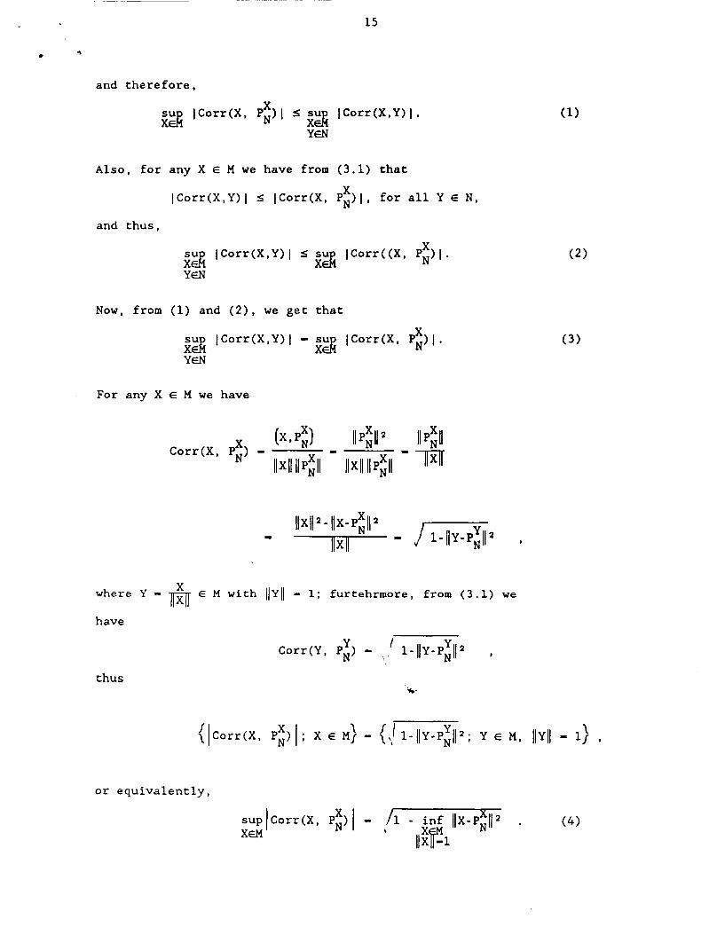
and therefore, X ICorr(X, PN)l 4 ;% ICorr(X,Y)l.
YEN ;%
A l s o , for any X E M we have from (3.1) that X ICorr(X,Y)I 5 ICorr(X, PN)I, for all Y E N,
and thus, ..
Now, from (1) and ( 2 ) , we get that
YEN
For any X E M we have
E M with llYll - 1; furtehrmore, f r o m (3.1) we m where Y - have
thus i-
or equivalently,
16
The desired result, now, follows from ( 3 ) and ( 4 ) . I
Proof of Lemma 3.2: The sequence CpmI is bounded and nondecreasing,
thus it is convergent and, in fact,
A l s o , since the linear span of F, is a subset of that of F, we have
pm 5 p , for all m 2 1,
and therefore,
Jim pm 5 p . m
To establish equalitly in (2 ) , note that for any two finite linear n m
combinations X - C akXt,k, Y - C bkXt+k, we have k-0 k-1
By taking supremum of both sides of ( 3 ) , over all X and Y as above,
we arrive at
The desired result, now, follows from (l), ( 2 ) and (4). Proof of (b) is
similar to (a). i-

References
h i k e , H. (1975). Markovian representation of stochastic processes by canonical variables. SIAM J. Control 13, 162-173.
Helson, H., Szeg6, G. (1960). A problem in prediction theory. Ann. Mat. Pura. Appl. - 51, 107-138.
Jewell, N.P., Bloomfield, P., Bartmann, F.C. (1983). Canonical correlations of past and future for time series: Bounds and computation. Ann. Statist. 11, 848-855.
Jewell, N.P., Bloomfield, P. (1983). Canonical correlations of past and future for time series: Definitions and theory. Ann. Statist. - 11, 837-847.
Johnson, R.A., Wichern, D.W. (1988). Applied Multivariate Statistical Analysis. Prentice Hall, New Jersey.
Piccolo, D., Tunnicliffe Wilson, G. (1984). A unified approach to ARMA model identification and preliminary estimation. J. of Time Series Analysis, 5, 183-204.
Pourahmadi, M. (1985). A matricial extension of the Helson-Szeg6 theorem and its applications in multivariate prediction. J. of Multivariate Analysis, 16, 265-275.
Rao, C.R. (1973). Linear Statistical Inference and Its Applications. John Wiley & Sons, New York.
Tsay, R.S., Tiao, G.C. (1985). Use of canonical analysis in time series model identification. Biometrika 72, 299-315.
Yaglom, A.M. (1965). Stationary Gaussian processes satisfying the strong mixing condition and best predictable functionals. Seminar of the Statistical Laboratory, University of California, Berkeley, 1963, 241-252. Springer-Verlag, New York.
Proc, Int. Research


![Rational Canonical Formbuzzard.ups.edu/...spring...canonical-form-present.pdfIntroductionk[x]-modulesMatrix Representation of Cyclic SubmodulesThe Decomposition TheoremRational Canonical](https://static.fdocuments.us/doc/165x107/6021fbf8c9c62f5c255e87f1/rational-canonical-introductionkx-modulesmatrix-representation-of-cyclic-submodulesthe.jpg)