J Algebr Comb (2012) 35:19–59DOI 10.1007/s10801-011-0292-6

Cohomology of GKM fiber bundles

Victor Guillemin · Silvia Sabatini · Catalin Zara

Received: 5 April 2010 / Accepted: 14 April 2011 / Published online: 12 May 2011© Springer Science+Business Media, LLC 2011

Abstract The equivariant cohomology ring of a GKM manifold is isomorphic to thecohomology ring of its GKM graph. In this paper we explore the implications of thisfact for equivariant fiber bundles for which the total space and the base space are bothGKM and derive a graph theoretical version of the Leray–Hirsch theorem. Then weapply this result to the equivariant cohomology theory of flag varieties.

Keywords Equivariant fiber bundle · Equivariant cohomology · GKM space · Flagmanifold

1 Introduction

Let T be an n-dimensional torus, and M a compact, connected T -manifold.The equivariant cohomology ring of M , H ∗

T (M;R), is an S(t∗)-module, whereS(t∗) = H ∗

T (point) is the symmetric algebra on t∗, the dual of the Lie algebra of T .If H ∗

T (M) is torsion-free, the restriction map

i∗ : H ∗T (M) → H ∗

T

(MT

)

V. GuilleminDepartment of Mathematics, MIT, Cambridge, MA 02139, USAe-mail: vwg@math.mit.edu

S. SabatiniDepartment of Mathematics, EPFL, Lausanne, Switzerlande-mail: silvia.sabatini@epfl.ch

C. Zara (�)Department of Mathematics, UMass Boston, Boston, MA 02125, USAe-mail: czara@math.umb.edu

20 J Algebr Comb (2012) 35:19–59

is injective and hence computing H ∗T (M) reduces to computing the image of H ∗

T (M)

in H ∗T (MT ). If MT is finite, then

H ∗T

(MT

) =⊕

p∈MT

S(t∗),

with one copy of S(t∗) for each p ∈ MT . Determining where H ∗T (M) sits inside this

sum is a challenging problem. However, one class of spaces M with H ∗T (M) torsion-

free for which this problem has a simple and elegant solution is the one introducedby Goresky–Kottwitz–MacPherson in their seminal paper [6]. These are now knownas GKM spaces: an equivariantly formal space M is a GKM space if MT is finite andfor every codimension one subtorus T ′ ⊂ T , the connected components of MT ′

areeither points or 2-spheres.

To each GKM space M we attach a graph Γ = ΓM by decreeing that the points ofMT are the vertices of Γ and the edges of Γ are these two-spheres. If S is one of theedge two-spheres, then ST consists of exactly two T -fixed points, p and q . If M hasan invariant almost complex or symplectic structure, then the isotropy representationson tangent spaces at fixed points are complex representations and their weights arewell-defined. These data determine a map

α : EΓ → Z∗T

of oriented edges of Γ into the weight lattice of T . This map assigns to the edge2-sphere S with North pole p the weight of the isotropy representation of T on thetangent space to S at p. The map α is called the axial function of the graph Γ .We use it to define a subring H ∗

α (ΓM) of H ∗T (MT ) as follows. Let c be an ele-

ment of H ∗T (MT ), i.e. a function which assigns to each p ∈ MT an element c(p)

of H ∗T (point) = S(t∗). Then c is in H ∗

α (ΓM) if and only if for each edge e of ΓM

with vertices p and q as end points, c(p) ∈ S(t∗) and c(q) ∈ S(t∗) have the same im-age in S(t∗)/αeS(t∗). (Without the invariant almost complex or symplectic structure,the isotropy representations are only real representations and the weights are definedonly up to sign; however, that does not change the construction of H ∗

α (Γ ).) A con-sequence of a Chang–Skjelbred result ([4]) is that H ∗

α (ΓM) is the image of i∗, andtherefore there is an isomorphism of rings

H ∗T (M) � H ∗

α (ΓM). (1.1)

In a companion paper [13] we prove a fiber bundle generalization of this result. LetM and B be T -manifolds and π : M → B be a T -equivariant fiber bundle. If H ∗

T (M)

is torsion-free, then the restriction map

i∗ : H ∗T (M) → H ∗

T

(π−1(BT )

)

is injective, and if BT is finite then H ∗T (π−1(BT )) is isomorphic to

⊕

p∈BT

H ∗T (Fp) (1.2)

J Algebr Comb (2012) 35:19–59 21

with Fp = π−1(p). We show in [13] that if B is GKM, then the image of H ∗T (M) in

(1.2) can be computed by a generalized version of (1.1). Moreover, if the fiber bundleis balanced (as defined in [13]), there is a holonomy action of the groupoid of pathsin Γ on the sum (1.2) and the elements which are invariant under this action form aninteresting subring of H ∗

T (M).In this paper we will take the analysis of H ∗

T (M) one step further by assumingthat M is also GKM. By interpreting this assumption combinatorially one is led toa combinatorial notion which is a central topic of this paper, the notion of a “fiberbundle of a GKM graph (Γ1, α1) over a GKM graph (Γ2, α2),” and, associated withthis, the notion of a “holonomy action” of the groupoid of paths in Γ2 on the ringHα1(Γ1). We will explore below the properties of such fiber bundles and apply theseresults to fiber bundles between generalized flag varieties; i.e. fiber bundles of theform

π : G/P1 → G/P2, (1.3)

where G is a semi-simple Lie group and P1 and P2 are parabolic subgroups. In par-ticular we will examine in detail the fiber bundle

π : F l(C

n) → Grk

(C

n), (1.4)

of complete flags in Cn over the Grassmannian of k-dimensional subspaces of C

n

and the analogue of this fibration for the classical groups of type Bn, Cn, and Dn. Foreach of these examples we will compute the subring of invariant classes in H ∗

T (M)

(those elements which are fixed by the holonomy action of the paths in Γ2) and showhow the generators of this ring are related to the usual basis of H ∗

T (M), given byequivariant Schubert classes. These results were inspired by and are related to resultsof Sabatini and Tolman. In [18] they explore the equivariant cohomology of fiber bun-dles where the total space and the base space are more general symplectic manifoldswith Hamiltonian actions. The theory developed in the present paper can be regardedas a combinatorial version of the geometrical theory of symplectic fibrations of coad-joint orbits, studied in [11].

What follows is a brief table of contents for this paper: In Sect. 2.1 we describesome of the salient features of the fiber bundle (1.4). In Sects. 2.2–2.4 we briefly re-view the theory of abstract GKM graphs, following [9], [10], and [7]. We then defineabstract versions of fibrations and fiber bundles between GKM graphs which incor-porate these features, and in Sects. 3.1–3.3 we show how to compute the cohomologyring of such graphs. The main ingredient in this computation is a holonomy action ofthe group of based loops in the base on the cohomology of the fiber graph.

In Sect. 4 we apply this theory to generalized flag manifolds, which have beenextensively studied in the combinatorics literature, but not from the perspective ofthis paper. Let G be a semisimple Lie group, B a Borel subgroup of G and P1 ⊂ P2

parabolic subgroups containing B . Building on results of [12], in Sect. 4.1 we de-scribe the GKM graph associated with the space P2/P1. In Sects. 4.3–4.4 we discussthe fibration of GKM graphs associated with the fibration of T -manifolds (1.3) andcompute the group of holonomy automorphisms associated with this fibration. InSect. 5 we specialize to the case where G is one of the four classical simple Lie

22 J Algebr Comb (2012) 35:19–59

group types, An, Bn, Cn, or Dn, and, using iterations of fiber bundles, give explicitconstructions of bases of invariant classes.

In Sect. 6 we construct a second explicit basis of H ∗T (G/B) consisting of classes

that are W -invariant. These invariant classes are obtained from the equivariant Schu-bert classes by averaging over the action of the Weyl group. In Theorem 6.1 we giveexplicit combinatorial formulas for the decomposition of twisted Schubert classes,generalizing earlier results of Tymoczko ([19, Theorem 4.9]) from twistings by sim-ple reflections to actions of general Weyl group elements. We then obtain formulas forthe transition matrix between the basis of invariant classes consisting of symmetrizedSchubert classes and the basis of invariant classes obtained through the iterated fiberbundle construction. In addition we obtain an explicit formula for the decompositionof an invariant class in the basis of equivariant Schubert classes.

2 GKM fiber bundles

2.1 Motivating example

Let T n = (S1)n be the compact torus of dimension n, with Lie algebra tn = Rn,

and let {x1, . . . , xn} be the basis of t∗n � Rn dual to the canonical basis of R

n. Let{e1, . . . , en} be the canonical basis of C

n. The torus T n acts componentwise on Cn

by

(t1, . . . , tn) · (z1, . . . , zn) = (t1z1, . . . , tnzn).

This action induces a T n-action on both M = F l(Cn), the manifold of complete flagsin C

n, and B = Grk(Cn), the Grassmannian manifold of k-dimensional subspaces

of Cn. Let C = {(t, . . . , t) | t ∈ S1} be the diagonal circle in T n and let T = T n/C.

Then C acts trivially on the flag manifold and on Grassmannians, and the inducedactions of T on F l(Cn) and on Grk(C

n) are effective. Let

π : F l(C

n) → Grk

(C

n), (2.1)

be the map that sends each complete flag V• = (V1, . . . , Vn) to its k-dimensionalcomponent. Then (M,B,π) is a T -equivariant fiber bundle.

Since flag manifolds and Grassmannians are GKM spaces, their T -equivariantcohomology rings are determined by fixed point data. These data can be nicely orga-nized using the corresponding GKM graphs, as follows. For a general GKM space M

the fixed point set MT is finite and is the vertex set of the GKM graph Γ . If T ′ ⊂ T isa codimension one subtorus of T , then the connected components of the set MT ′

ofT ′-fixed points are either T -fixed points or copies of CP 1 joining two T -fixed points.The edges of the graph Γ correspond to these CP 1’s, for all codimension one subtoriT ′ ⊂ T . An edge e corresponding to a connected component of MT ′

is labeled by anelement αe ∈ t∗ such that t′ = kerαe . As explained in the introduction, the equivariantcohomology ring H ∗

T (M) can be computed from the GKM graph (Γ,α) associatedto M , and we will give the details of that construction in Sect. 3.1.

J Algebr Comb (2012) 35:19–59 23

Fig. 1 The complete graph K3(a) and the Cayley graph(S3, t) (b)

For the flag manifold F l(Cn), the T -fixed point set is indexed by Sn, the group ofpermutations of [n] = {1, . . . , n}. A permutation u = u(1) . . . u(n) of [n] indexes thefixed flag

V u• = (V u

1 , . . . , V un

),

given by V uk = Ceu(1) ⊕ · · · ⊕ Ceu(k), for all k = 1, . . . , n.

The codimension one subtori T ′ of T for which the fixed point set is not just theset of T -fixed points are the subtori Tij = {t ∈ T | ti = tj } = exp (ker(xi − xj )). Fora fixed flag V u• , the connected component of F l(Cn)Tij that passes through V u• alsocontains the fixed flag V v• , where v = (i, j)u and (i, j) is the transposition that swapsi and j .

The GKM graph Γ of the flag manifold F l(Cn) is the Cayley graph (Sn, t) con-structed from the group Sn and generating set t , the set of transpositions: the verticescorrespond to permutations in Sn and two vertices are joined by an edge if they differby a transposition. If u ∈ Sn, then u ∗ (i, j) = (u(i), u(j)) ∗ u, so two permutationsthat differ by a transposition on the right (operating on positions) also differ by atransposition on the left (operating on values). We denote the edge e that joins u andv = u ∗ (i, j) by u → v. If 1 � i < j � n, then the value of the axial function α onthis edge is

αe = xu(i) − xu(j).

We will refer to Γ as Sn, and it will be clear from the context when Sn is the graph, thevertex set, or the group of permutations. Figure 1(b) shows the Cayley graph (S3, t).As a general convention throughout this paper, edges that are represented by parallelsegments have collinear labels. For example, α(123,132) = α(231,321) = x2 − x3.

For the Grassmannian Grk(Cn), the T -fixed point set is indexed by k-element sub-

sets of [n]. A subset I = {i1, . . . , ik} corresponds to the fixed k-dimensional subspaceVI = Cei1 ⊕· · ·⊕Ceik . Two vertices are joined by an edge if the intersection of theircorresponding k-element subsets is a (k − 1)-element subset. The resulting graph isthe Johnson graph J (n, k). If I = (I ∩ J ) ∪ {i} and J = (I ∩ J ) ∪ {j}, then the valueof the axial function on the edge e from I to J is αe = xi − xj . In particular, whenk = 1 we get the complex projective space CP n−1, and the associated graph is thecomplete graph Kn with n vertices. The complete graph K3 is shown in Fig. 1(a).

The discrete version of (2.1) is the morphism of graphs π : Sn → J (n, k), givenby π(u) = {u(1), . . . , u(k)}. This map is compatible with the axial functions on the

24 J Algebr Comb (2012) 35:19–59

Fig. 2 The GKM fiber bundleS4 → J (4,2)

two graphs, and for each vertex A ∈ J (n, k), the fiber π−1(A) is a product Sk ×Sn−k .The axial functions on fibers are not identical, but they are compatible in a naturalway.

The GKM fiber bundle S4 → J (4,2) is a combinatorial description of the fiberbundle F l4(C) → Gr2(C

4) that sends a complete flag in F l4(C) to its two dimen-sional component. Figure 2 shows the graphical representation of this fiber bundle.The fibers are the squares. (The internal edges of S4 have been omitted.)

This example motivates one of the main goals of this paper: to define the discreteanalog of a fiber bundle between GKM spaces for which the fibers are isomorphicGKM spaces. We then prove a discrete Leray–Hirsch theorem, showing how one canrecover the graph cohomology of the total space from the cohomology of the baseand invariant classes in the cohomology of the fiber.

Then we will revisit the example π : F l(Cn) → Grk(Cn) and consider more

general fiber bundles G/B → G/P , with B ⊂ P ⊂ G a Borel and parabolic sub-group of a complex semisimple Lie group G, and give a combinatorial descrip-tion/construction of invariant classes for classical groups.

2.2 Abstract GKM graphs

We start by recalling some general definitions (see [9, 10] for more details and mo-tivation). The reader should have in mind the examples of the Cayley graph Sn, thecomplete graph Kn, and the Johnson graph J (n, k). We will return to these with asummarizing example at the end of Sect. 2.

Let Γ = (V ,E) be a regular graph, with V the set of vertices and E the set oforiented edges. We will consider oriented edges, so each unoriented edge e joiningvertices p and q will appear twice in E: once as (p, q) = p → q and a second timeas (q,p) = q → p. When e is oriented from p to q , we will call p = i(e) the initialvertex of e, and q = t (e) the terminal vertex of e. For a vertex p, let Ep be the set oforiented edges with initial vertex p.

J Algebr Comb (2012) 35:19–59 25

Definition 2.1 Let e = (p, q) be an edge of Γ , oriented from p to q . A connectionalong the edge e is a bijection ∇e : Ep → Eq such that ∇e(p, q) = (q,p). A con-nection on Γ is a family ∇ = (∇e)e∈E of connections along the oriented edges of Γ ,such that ∇(q,p) = ∇−1

(p,q) for every edge e = (p, q) of Γ .

Definition 2.2 Let ∇ be a connection on Γ . A ∇-compatible axial function on Γ isa labeling α : E → t∗ of the oriented edges of Γ by elements of a linear space t∗,satisfying the following conditions:

1. α(q,p) = −α(p,q);2. For every vertex p, the vectors {α(e) | e ∈ Ep} are mutually independent;3. For every edge e = (p, q), and for every e′ ∈ Ep we have

α(∇e(e

′)) − α(e′) = cα(e),

for some scalar c ∈ R that depends on e and e′.

An axial function on Γ is a labeling α : E → t∗ that is a ∇-compatible axial functionfor some connection ∇ on Γ .

Definition 2.3 A GKM graph is a pair (Γ,α) consisting of a regular graph Γ and anaxial function α : E → t∗ on Γ .

Example 2.1 (The complete graph) For the complete graph Γ = Kn considered inSect. 2.1, the axial function on oriented edges is defined as follows. Let t∗ be ann-dimensional linear space and {x1, . . . , xn} be a basis of t∗. Define α : E → t∗ by

α(i, j) = xi − xj .

If ∇(i,j) : Ei → Ej sends (i, j) to (j, i) and (i, k) to (j, k) for k �= i, j , then ∇ is aconnection compatible with α. The image of α spans the (n − 1)-dimensional sub-space t∗0 generated by α1 = x1 − x2, . . . , αn−1 = xn−1 − xn.

When n = 2, the graph Γ has two vertices, 1 and 2, joined by an edge. The ori-ented edge from 1 to 2 is labeled β = x1 − x2, and the oriented edge from 2 to 1 islabeled −β = x2 − x1. The second condition in the definition of an axial function isautomatically satisfied.

Example 2.2 (The Cayley graph (Sn, t)) For the Cayley graph Γ = (Sn, t) consideredin Sect. 2.1, the axial function on oriented edges is defined as follows. Let t∗ bean n-dimensional linear space and {x1, . . . , xn} be a basis of t∗. Let α : E → t∗ bethe axial function defined as follows. If u → v = u(i, j) is an oriented edge, with1 � i < j � n, define

α(u, v) = xu(i) − xu(j).

Note that α(u, v) is determined by the values changed from u to v. For an edgee = u → v = u(i, j), define ∇e : Eu → Ev by

∇e

(u,u(a, b)

) = (v, v(a, b)

). (2.2)

26 J Algebr Comb (2012) 35:19–59

Then ∇ is a connection compatible with α and, as above, the image of α spans the(n − 1)-dimensional subspace t∗0 generated by α1 = x1 − x2, . . . , αn−1 = xn−1 − xn.

The examples above show that the image of α may not generate the entire linearspace t∗. Let (Γ,α) be a GKM graph. For a vertex p, let

t∗p = span{αe | e ∈ Ep} ⊂ t

∗

be the subspace of t∗ generated by the image of the axial function on edges withinitial vertex p. If Γ is connected, then this subspace is the same for all verticesof Γ , and we will denote it by t∗0. We can co-restrict the axial function α : E → t∗ toa function α0 : E → t∗0, and the resulting pair (Γ,α0) is also a GKM graph.

Definition 2.4 An axial function α : E → t∗ is called effective if t∗0 = t∗.

Let (Γ,α) be a GKM graph with Γ = (V ,E) and axial function α : E → t∗. Let∇ be a connection compatible with α. Let Γ0 = (V0,E0) be a subgraph of Γ , withV0 ⊂ V and E0 ⊂ E, such that, if e ∈ E is an edge with i(e), t (e) ∈ V0, then e ∈ E0.

Definition 2.5 The connected subgraph Γ0 is a ∇-GKM subgraph if for every edgee ∈ E0 with i(e) = p and t (e) = q , we have ∇e(Ep ∩ E0) = Eq ∩ E0. The subgraphΓ0 is a GKM subgraph if it is a ∇-GKM subgraph for a connection ∇ compatiblewith α.

In other words, Γ0 is a GKM subgraph if, for some connection ∇ compatible withthe axial function α, the connection along edges of Γ0 sends edges of Γ0 to edges ofΓ0 and edges not in Γ0 to edges not in Γ0. Then the connected subgraph Γ0 is regular,the restriction α0 of α to E0 is an axial function on Γ0, and the connection ∇ inducesa connection ∇0 compatible with α0. Therefore a GKM subgraph is naturally a GKMgraph.

2.2.1 Isomorphisms of GKM Graphs

Let (Γ1, α1) and (Γ2, α2) be two GKM graphs, with Γ1 = (V1,E1), α1 : E1 → t∗1 andΓ2 = (V2,E2), α2 : E2 → t∗2.

Definition 2.6 An isomorphism of GKM graphs from (Γ1, α1) to (Γ2, α2) is a pair(Φ,Ψ ), where

1. Φ : Γ1 → Γ2 is an isomorphism of graphs;2. Ψ : t∗1 → t∗2 is an isomorphism of linear spaces;3. For every edge (p, q) of Γ1 we have

α2(Φ(p),Φ(q)

) = Ψ ◦ α1(p, q).

J Algebr Comb (2012) 35:19–59 27

The first condition implies that Φ induces a bijection from E1 to E2, and the thirdcondition can be restated as saying that the following diagram commutes:

E1Φ

α1

E2

α2

t∗1Ψ

t∗2

2.3 Fiber bundles of graphs

We now introduce special types of morphisms between graphs. Later we will add theGKM package (axial function and connection) and define the corresponding types ofmorphisms between GKM graphs.

2.3.1 Fibrations

Let Γ and B be connected graphs and π : Γ → B be a morphism of graphs. By thiswe mean that π is a map from the vertices of Γ to the vertices of B such that, if(p, q) is an edge of Γ , then either π(p) = π(q) or else (π(p),π(q)) is an edge of B .

When (p, q) is an edge of Γ and π(p) = π(q), we will say that the edge (p, q) isvertical; otherwise (π(p),π(q)) is an edge of B and we will say that (p, q) is hori-zontal. For a vertex q of Γ , let E⊥

q be the set of vertical edges with initial vertex q ,and let Hq be the set of horizontal edges with initial vertex q . Then Eq = E⊥

q ∪ Hq

and π canonically induces a map (dπ)q : Hq → (EB)π(q) given by

(dπ)q(q, q ′) = (π(q),π(q ′)

). (2.3)

Definition 2.7 The morphism of graphs π : Γ → B is a fibration of graphs1 if forevery vertex q of Γ , the map (dπ)q : Hq → (EB)π(q) is bijective.

Fibrations have the unique lifting of paths property: Let π : Γ → B be a fibra-tion, (p0,p1) an edge of B , and q0 ∈ π−1(p0) a point in the fiber over p0. Since(dπ)q0 : Hq0 → (EB)p0 is a bijection, there exists a unique edge (q0, q1) such that(dπ)q0(q0, q1) = (p0,p1). We will say that (q0, q1) is the lift of (p0,p1) at q0. If γ

is a path p0 → p1 → ·· · → pm in B and q0 ∈ π−1(p0) is a point in the fiber over p0,then we can lift γ uniquely to a path γ (q0) = q0 → q1 → ·· · → qm in Γ starting atq0, by successively lifting the edges of γ .

2.3.2 Fiber bundles

Let π : Γ → B be a fibration of graphs. For a vertex p of B , let Vp = π−1(p) ⊂ V

and let Γp be the induced subgraph of Γ with vertex set Vp . For every edge (p, q)

1This is what we called submersion in [10]. This definition of a fibration of graphs is different from the oneintroduced in [3]. We work with undirected graphs, and our morphisms of graphs allow edges to collapse.

28 J Algebr Comb (2012) 35:19–59

Fig. 3 Twisted fibration

of B , define a map Φp,q : Vp → Vq as follows. For p′ ∈ Vp , define Φp,q(p′) = q ′,where (p′, q ′) is the lift of (p, q) at p′. It is easy to see that Φp,q is bijective, withinverse Φq,p . What is not true, in general, is that Φp,q is an isomorphism of graphsfrom Γp to Γq .

Example 2.3 Let Γ be the regular 3-valent graph consisting of two quadrilaterals(p1,p2,p3,p4) and (q1, q3, q2, q4) joined by edges (pi, qi) for i = 1,2,3,4. (SeeFig. 3.)

Let B be a graph with two vertices p and q joined by an edge. Let π : Γ → B

be the morphism of graphs π(pi) = p and π(qi) = q for i = 1,2,3,4. Then π is afibration and Φp,q(pi) = qi for i = 1,2,3,4. However, (p1,p2) is an edge in Γp , but(q1, q2) is not an edge in Γq . While the fibers Γp and Γq are isomorphic as graphs,the map Φp,q is not an isomorphism.

We will be interested in fibrations for which Φp,q is an isomorphism of graphsfrom the fiber Γp to the fiber Γq .

Definition 2.8 A fibration π : Γ → B is a fiber bundle2 if for every edge (p, q) ofB , the map Φp,q : Γp → Γq is a morphism of graphs.

If π : Γ → B is a fiber bundle then Φp,q is bijective, and both Φp,q : Γp → Γq

and Φ−1p,q = Φq,p : Γq → Γp are morphisms of graphs. Therefore the maps Φp,q are

isomorphisms of graphs. The simplest example of a fiber bundle is the projection ofa direct product of graphs onto one of its factors, π : Γ = B × F → B . We will callsuch fiber bundles trivial bundles.

2.4 GKM fiber bundles

We now add the GKM package to a fibration, and define GKM fibrations. Let (Γ,α)

and (B,αB) be two GKM graphs, with axial functions α : E → t∗ and αB : EB → t∗taking values in the same linear space t∗. Let ∇ and ∇B be connections on Γ and B ,compatible with α and αB , respectively.

2This is what we called fibration in [10].

J Algebr Comb (2012) 35:19–59 29

Definition 2.9 A map π : (Γ,α) → (B,αB) is a (∇,∇B)-GKM fibration if it satisfiesthe following conditions:

1. π is a fibration of graphs;2. If e is an edge of B and e is any lift of e, then α(e) = αB(e);3. Along every edge e of Γ the connection ∇ sends horizontal edges into horizontal

edges and vertical edges into vertical edges;4. The restriction of ∇ to horizontal edges is compatible with ∇B , in the following

sense: Let e = (p, q) be an edge of B and e = (p′, q ′) the lift of e at p ′. Lete′ ∈ Ep and e′′ = (∇B)e(e

′) ∈ Eq . If e′ is the lift of e′ at p ′ and e′′ is the lift of e′′at q ′ then

(∇ )e(e′) = e′′.

A map π : (Γ,α) → (B,αB) is a GKM fibration if it is a (∇,∇B)-GKM fibration forsome connections ∇ and ∇B compatible with α and αB .

If π : (Γ,α) → (B,αB) is a GKM fibration, then for each p ∈ B , the fiber (Γp,α)

is a GKM subgraph of (Γ,α). Let v∗p be the subspace of t∗ generated by values

of axial functions αe , for edges e of Γp . Then the axial function on Γp can be co-restricted to αp , from the oriented edges of Γp to v∗

p , and (Γp,αp) is a GKM graph.Suppose now that π is both a GKM fibration and a fiber bundle of graphs. Let

e = (p, q) be an edge of B . We say that the transition isomorphism Φp,q : Γp → Γq

is compatible with the connection on Γ if for every lift e = (p1, q1) of e and forevery edge e′ = (p1,p2) of Γp , the connection along e moves e′ into the edgee′′ = (q1, q2) = (Φp,q(p1),Φp,q(p2)) of Γq .

Definition 2.10 A GKM fibration π : (Γ,α) → (B,αB) is a GKM fiber bundle if π

is a fiber bundle and for every edge e = (p, q) of B:

1. The transition isomorphism Φp,q is compatible with the connection of Γ .2. There exists a linear isomorphism Ψp,q : v∗

p → v∗q such that

Υp,q = (Φp,q,Ψp,q) : (Γp,αp) → (Γq,αq)

is an isomorphism of GKM graphs.

For a GKM fiber bundle π : (Γ,α) → (B,αB) we can be more specific about thetransition isomorphisms Ψp,q . Let (p, q) be an edge of B , let (p′,p′′) be an edgeof Γp , and let (q ′, q ′′) be the corresponding edge of Γq . The compatibility conditionalong the edge (p′, q ′) implies that αq ′,q ′′ − αp′,p′′ is a multiple of αp′,q ′ = αp,q ,hence there exists a unique constant c = c(αp′,p′′) such that

Ψp,q(αp ′,p ′′) = αp ′,p ′′ + c(αp′,p′′)αp,q .

The linearity of Ψp,q implies that there exists a unique linear function c : v∗p → R

such that

Ψp,q(x) = x + c(x)αp,q

30 J Algebr Comb (2012) 35:19–59

for all x ∈ v∗p .

For a path γ : p0 → p1 → ·· · → pm−1 → pm in B from p0 to pm, let

Υγ = Υpm−1,pm ◦ · · · ◦ Υp0,p1 : (Γp0 , αp0) → (Γpm,αpm)

be the GKM graph isomorphism given by the composition of the transition maps. Letp ∈ B be a vertex, and let Ω(p) be the set of all loops in B that start and end at p.If γ ∈ Ω(p) is a loop based at p, then Υγ is an automorphism of the GKM graph(Γp,αp). The holonomy group of the fiber Γp is the group

Holπ (Γp) = {Υγ | γ ∈ Ω(p)

}� Aut(Γp,αp).

If the base B is connected, then all the fibers are isomorphic as GKM graphs.Let (F,αF ) be a GKM graph isomorphic to all fibers, with αF : EF → t∗F , and, foreach vertex p of B , let ρp = (ϕp,ψp) : (F,αF ) → (Γp,α) be a fixed isomorphismof GKM graphs. For every edge (p,p ′) of B , let

ρp,p ′ = (ϕp,p ′ ,ψp,p ′) : (F,αF ) → (F,αF )

be the automorphism of (F,αF ) given by

ϕp,p ′ = ϕ−1p ′ ◦ Φp,p ′ ◦ ϕp,

ψp,p ′ = ψ−1p ′ ◦ Ψp,p ′ ◦ ψp.

If γ is any path in B , then the composition of the transition maps along the edges ofγ defines an automorphism ργ = (ϕγ ,ψγ ) of (F,αF ). Let p be a vertex of B and

Hol(F,p) = {ργ | γ ∈ Ω(p)

} ⊂ Aut(F,αF ).

Then Hol(F,p) is a subgroup of Aut(F,αF ) and if p,p ′ are vertices of B , thenHol(F,p) and Hol(F,p ′) are conjugated by ργ , where γ is any path in B connectingp and p ′.

2.5 Example

In this section we return to π : F l(Cn) → CP n−1 (as a particular case ofF l(Cn) → Grk(C

n)). We show that the discrete version, π : Sn → Kn, given byπ(u) = u(1), is an abstract GKM fiber bundle.

2.5.1 π is a GKM fibration

Clearly π is a morphism of graphs, because in Kn all vertices are joined by edges.Moreover, let u and v = u(i, j) (with 1 � i < j � n) be adjacent vertices in Sn.If i �= 1, then π(u) = π(v), hence the edge u → v is vertical. If i = 1, thenπ(v) = u(j) �= u(1), hence the edge u → v is horizontal.

Let (dπ)u : Hu → Eπ(u) be the induced map (2.3). If e is the horizontal edgeu → v = u(1, j), then (dπ)u(e) = e, the edge of Kn joining u(1) and u(j). Therefore(dπ)u is bijective, hence π is a fibration of graphs.

J Algebr Comb (2012) 35:19–59 31

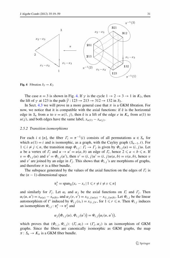
Fig. 4 Fibration S3 → K3

The case n = 3 is shown in Fig. 4. If γ is the cycle 1 → 2 → 3 → 1 in K3, thenthe lift of γ at 123 is the path γ : 123 → 213 → 312 → 132 in S3.

In Sect. 4.3 we will prove in a more general case that π is a GKM fibration. Fornow, we notice that it is compatible with the axial functions: if e is the horizontaledge in Sn from u to v = u(1, j), then e is a lift of the edge e in Kn from u(1) tou(j), and both edges have the same label, xu(1) − xu(j).

2.5.2 Transition isomorphisms

For each i ∈ [n], the fiber Γi = π−1(i) consists of all permutations u ∈ Sn forwhich u(1) = i and is isomorphic, as a graph, with the Cayley graph (Sn−1, t). For1 � i �= j � n, the transition map Φi,j : Γi → Γj is given by Φi,j (u) = (i, j)u. Letu be a vertex of Γi and u → u′ = u(a, b) an edge of Γi , hence 2 � a < b � n. Ifv = Φi,j (u) and v′ = Φi,j (u

′), then v′ = (i, j)u′ = (i, j)u(a, b) = v(a, b), hence v

and v′ are joined by an edge in Γj . This shows that Φi,j ’s are morphisms of graphs,and therefore π is a fiber bundle.

The subspace generated by the values of the axial function on the edges of Γi isthe (n − 1)-dimensional space

v∗i = spanR{xr − xs |1 � r �= i �= s � n}

and similarly for Γj . Let αi and αj be the axial functions on Γi and Γj . Thenαi(u,u′) = xu(a) − xu(b), and αj (v, v′) = x(i,j)u(a) − x(i,j)u(b). Let Ψi,j be the linearautomorphism of t∗ induced by Ψi,j (xr ) = x(i,j)r , for 1 � r � n. Then Ψi,j inducesan isomorphism Ψi,j : v∗

i → v∗j and

αj

(Φi,j (u),Φi,j (u

′)) = Ψi,j

(αi(u,u′)

),

which proves that (Φi,j ,Ψi,j ) : (Γi, αi) → (Γj ,αj ) is an isomorphism of GKMgraphs. Since the fibers are canonically isomorphic as GKM graphs, the mapπ : Sn → Kn is a GKM fiber bundle.

32 J Algebr Comb (2012) 35:19–59

2.5.3 Typical fiber

For 1 � i � n, the fiber (Γi, αi) is isomorphic to Sn−1, and we construct an explicitisomorphism ϕi : Sn−1 → Γi . For a permutation u ∈ Sn−1, let

u = u(1)u(2) · · ·u(n−1)n ∈ Sn.

For 1 � a < b � n, let ca,b be the cycle a → a + 1 → ·· · → b → a, and letcb,a = c−1

a,b . Then the map ϕi : Sn−1 → Γi ,

ϕi(u) = ci,nucn,1

is a graph isomorphism between Sn−1 and Γi . The cycle ci,n, operating on values,moves the value i to the last position and preserves the relative order of the valueson the other positions. The cycle cn,1, operating on positions, moves i from the lastposition to the first and then shifts all the other positions to the right by one.

Let ψi be the linear isomorphism induced by ψi(xk) = xci,n(k) for all 1 � k � n. Ifu ∈ Sn−1 and v = u(a, b), with 1 � a < b � n−1, then

αi

(ϕi(u),ϕi(v)

) = ψi

(α(u, v)

),

hence (ϕi,ψi) : Sn−1 → Γi is an isomorphism of GKM graphs.

2.5.4 Holonomy action on the fiber

Let Hol(Γn) be the holonomy group of the fiber Γn. It is generated by compositions oftransition isomorphisms along loops in Kn based at n. Each such nontrivial loop canbe decomposed into triangles γij : n → i → j → n, and for such a triangle we have(j, n)(i, j)(n, i) = (i, j), hence the corresponding element of Hol(Γn) generated byγij is

Υγij= (Φγij

,Ψγij),

with Φγij(u) = (i, j)u and Ψγij

(xr ) = x(i,j)r .Since every permutation in Sn−1 can be decomposed into transpositions, it follows

that

Hol(Γn) = {Υw = (Φw,Ψw) | w ∈ Sn−1

} � Sn−1,

where, for a permutation w ∈ Sn−1, Φw : Γn → Γn is given by Φw(u) = wu, andΨw(xa) = xw(a).

Since the holonomy actions are conjugated, it follows that the holonomy group ofall fibers are isomorphic to Sn−1.

3 Cohomology of GKM fiber bundles

Let π : (Γ,α) → (B,αB) be a GKM fiber bundle, with typical fiber (F,αF ). Oneof the main goals of this paper is to describe how the cohomology ring of the totalspace (Γ,α) is determined by the cohomology rings of the base (B,αB) and the fiber(F,αF ) and the holonomy action of the base on the fiber. We start by recalling theconstruction of the cohomology ring of a GKM graph.

J Algebr Comb (2012) 35:19–59 33

3.1 Cohomology of GKM graphs

Let (Γ,α) be a GKM graph, with Γ = (V ,E) a regular graph and α : E → t∗ anaxial function. Let S(t∗) be the symmetric algebra of t∗; if {x1, . . . , xn} is a basis oft∗, then S(t∗) � R[x1, . . . , xn].

Definition 3.1 A cohomology class on (Γ,α) is a map ω : V → S(t∗) such that forevery edge e = (p, q) of Γ , we have

ω(q) ≡ ω(p) (mod αe). (3.1)

The compatibility condition (3.1) means that ω(q) − ω(p) = αef , for some ele-ment f ∈ S(t∗), and is equivalent to ω(q) = ω(p) on ker(αe). If ω and τ are coho-mology classes, then ω + τ and ωτ are also cohomology classes.

Definition 3.2 The cohomology ring of (Γ,α), denoted by H ∗α (Γ ), is the subring of

Maps(V ,S(t∗)) consisting of all the cohomology classes.

Moreover, H ∗α (Γ ) is a graded ring, with the grading induced by S(t∗). We say that

ω ∈ H ∗α (Γ ) is a class of degree 2k if for every p ∈ V , the polynomial ω(p) ∈ S

k(t∗)is homogeneous of degree k. (The fact that the class degree is twice the polynomialdegree is a consequence of the convention that elements of t∗ have degree 2.) IfHk

α(Γ ) is the space of classes of degree 2k, then

H ∗α (Γ ) =

⊕

k�0

H 2kα (Γ ).

If ω ∈ H ∗α (Γ ) and h ∈ S(t∗), then hω ∈ H ∗

α (Γ ), hence H ∗α (Γ ) is an S(t∗)-module;

it is in fact a graded S(t∗)-module.

Remark 3.1 The main motivation behind these constructions is the fact that if M is aGKM manifold and Γ = ΓM is its GKM graph, then Hodd

T (M) = 0 and H 2kT (M) �

H 2kα (Γ ).

Let (Γ0, α) be a GKM subgraph of (Γ,α). If f : V → S(t∗) is a cohomologyclass on Γ , then the restriction of f to V0 is a cohomology class on Γ0. Therefore theinclusion i : (Γ0, α) → (Γ,α) induces a ring morphism i∗ : H ∗

α (Γ ) → H ∗α (Γ0).

If ρ = (ϕ,ψ) : (Γ1, α1) → (Γ2, α2) is an isomorphism of GKM graphs, defineρ∗ : Maps(V2,S(t∗)) → Maps(V1,S(t∗)) by

(ρ∗(f )

)(p) = ψ−1(f

(ϕ(p)

)),

for p ∈ V1, where ψ−1 : S(t∗) → S(t∗) is the algebra isomorphism extending the lin-ear isomorphism ψ−1 : t∗ → t∗. Then ρ∗ is a ring isomorphism and (ρ∗)−1 = (ρ−1)∗,but, unless ψ : t∗ → t∗ is the identity, ρ∗ is not an isomorphism of S(t∗)-modules.

34 J Algebr Comb (2012) 35:19–59

3.2 Cohomology of GKM fiber bundles

Let π : (Γ,α) → (B,αB) be a GKM fiber bundle. For a cohomology classf : VB → S(t∗) on the base (B,αB), define the pull-back π∗(f ) : VΓ → S(t∗) byπ∗(f )(q) = f (π(q)). Then π∗(f ) is a cohomology class on (Γ,α), and π definesan injective morphism of rings π∗ : H ∗

αB(B) → H ∗

α (Γ ). In particular, H ∗α (Γ ) is an

H ∗αB

(B)-module.

Definition 3.3 A cohomology class h ∈ H ∗α (Γ ) is called basic if h ∈ π∗(H ∗

αB(B)).

Let (H ∗α (Γ ))bas = π∗(H ∗

αB(B)) ⊆ H ∗

α (Γ ). Then (H ∗α (Γ ))bas is a subring of

H ∗α (Γ ), and is isomorphic to H ∗

αB(B). We will identify H ∗

αB(B) and (H ∗

α (Γ ))basand regard H ∗

αB(B) as a subring of H ∗

α (Γ ).The next theorem is one of the main results of this paper, and shows how the

cohomology of the total space Γ is determined by the cohomology of the base B andspecial sets of cohomology classes with certain properties on fibers.

Theorem 3.1 Let π : (Γ,α) → (B,αB) be a GKM fiber bundle, and let c1, . . . , cm

be cohomology classes on Γ such that, for every p ∈ B , the restrictions of theseclasses to the fiber Γp = π−1(p) form a basis for the cohomology of the fiber. Then,as H ∗

αB(B)-modules, H ∗

α (Γ ) is isomorphic to the free H ∗αB

(B)-module on c1, . . . , cm.

Proof A linear combination of c1, . . . , cm with coefficients in (H ∗α (Γ ))bas � H ∗

αB(B)

is clearly a cohomology class on Γ . If such a combination is the zero class, then

m∑

k=1

βk(p)ck(p′) = 0

for every p ∈ B and p ′ ∈ Γp . Since the restrictions of c1, . . . , cm to Γp are indepen-dent, it follows that βk(p) = 0 for every k = 1, . . . ,m. This is valid for all p ∈ B ,hence the classes β1, . . . , βm are zero. Therefore c1, . . . , cm are independent overH ∗

αB(B), and the free H ∗

αB(B)-module they generate is a submodule of H ∗

α (Γ ).We prove that this submodule is the entire H ∗

α (Γ ). Let c ∈ H ∗α (Γ ) be a cohomol-

ogy class on Γ . For p ∈ B , the restriction of c to the fiber Γp is a cohomology classon Γp . Since the restrictions of c1, . . . , cm to Γp generate the cohomology of Γp , thereexist polynomials β1(p), . . . , βm(p) in S(t∗) such that, for every p ′ ∈ Γp ,

c(p ′) =m∑

k=1

βk(p)ck(p′).

We will show that the maps βk : B → S(t∗) are in fact cohomology classes on B . Lete = p → q be an edge of B , with weight αe = αpq ∈ t∗. Let p ′ ∈ Γp , and q ′ ∈ Γq besuch that p ′ → q ′ is the lift of p → q . Then α(p ′, q ′) = α(p,q) = αe and

c(q ′) − c(p ′) =m∑

k=1

(βk(q)ck(q

′) − βk(p)ck(p′))

J Algebr Comb (2012) 35:19–59 35

=m∑

k=1

(βk(q) − βk(p)

)ck(p

′) +m∑

k=1

βk(q)(ck(q

′) − ck(p′)).

Since c, c1, . . . , cm are classes on Γ , the differences c(q ′) − c(p ′), ck(q′) − ck(p

′)are multiples of αe , for all k = 1, . . . ,m. Therefore, for all p ′ ∈ Γp ,

m∑

k=1

(βk(q) − βk(p)

)ck(p

′) = αeη(p ′),

where η(p ′) ∈ S(t∗). We will show that η : Γp → S(t∗) is a cohomology class on Γp .If p ′ and p ′′ are vertices in Γp , joined by an edge (p ′,p ′′), then

m∑

k=1

(βk(q) − βk(p)

)(ck(p

′′) − ck(p′)) = αe

(η(p ′′) − η(p ′)

).

Each ck is a cohomology class on Γ , so ck(p′′) − ck(p

′) is a multiple of α(p ′,p ′′),for all k = 1, . . . ,m. Then αe(η(p ′′) − η(p ′)) is also a multiple of α(p ′,p ′′). Butαe = α(p ′, q ′) and α(p ′,p ′′) point in different directions as vectors, so, as linearpolynomials, they are relatively prime. Therefore η(p ′′) − η(p ′) must be a multipleof α(p ′,p ′′). Therefore η is a cohomology class on Γp .

The restrictions of c1, . . . , cm form a basis for the cohomology ring of Γp , hencethere exist polynomials Q1, . . . ,Qm ∈ S(t∗) such that

η(p ′) =m∑

k=1

Qkck(p′)

for all p ′ ∈ Γp . Then

m∑

k=1

(βk(q) − βk(p) − Qkαe

)ck = 0

on the fiber Γp . Since the classes c1, . . . , cm restrict to linearly independent classeson fibers, it follows that

βk(q) − βk(p) = Qkαe,

hence βk ∈ H ∗αB

(B). Therefore every cohomology class on Γ can be written as alinear combination of classes c1, . . . , cm, with coefficients in H ∗

αB(B). �

3.3 Invariant classes

In this section we describe a method of constructing global classes c1, . . . , cm withthe properties required by Theorem 3.1.

Let π : (Γ,α) → (B,αB) be a GKM fiber bundle, with typical fiber (F,αF ). Letp be a fixed vertex of B and let ρp = (ϕp,ψp) : (F,αF ) → (Γp,αp) be a GKM iso-morphism from F to the fiber above p. For a loop γ ∈ Ω(p), let ργ = (ϕγ ,ψγ )

36 J Algebr Comb (2012) 35:19–59

be the GKM automorphism of (F,αF ) determined by γ . Let K = Hol(F,p) bethe holonomy subgroup of Aut(F,αF ) generated by all automorphisms ργ , and letf ∈ (H ∗

αF(F ))K be a cohomology class on the fiber, invariant under all the automor-

phisms in K . Then fp = (ρ−1p )∗(f ) ∈ H ∗

α (Γp) is a class on the fiber over p, invariantunder all the automorphisms in Holπ (Γp) ⊂ Aut(Γp,α). For any vertex q ∈ Γp wehave fp(q) ∈ S(v∗

p) ⊂ S(t∗), where v∗p is the subspace of t∗ generated by the values

of α on the edges of Γp .We will extend the class fp from the fiber Γp to the total space Γ . Let p ′ be a

vertex of B , and γ a path in B from p ′ to p. Let Υ ∗γ : H ∗

α (Γp) → H ∗α (Γp ′) be the

ring isomorphism induced by the GKM graph isomorphism Υγ : (Γp ′ , α) → (Γp,α).Since fp is Holπ (Γp)-invariant, it follows that if γ1 and γ2 are two paths in B fromp ′ to p, then Υ ∗

γ1(fp) = Υ ∗

γ2(fp). We define fp′ = Υ ∗

γ (fp) ∈ H ∗α (Γp ′), where γ is

any path in B from p ′ to p. Then fp′(q ′) ∈ S(t∗p′) ⊂ S(t∗) for every q ′ ∈ Γp ′ .

Proposition 3.1 Let c = cf,p : VΓ → S(t∗) be defined by c|Γq = fq for all q ∈ B .Then c ∈ H ∗

α (Γ ).

Proof Since the restrictions of c to fibers are classes on fibers, it suffices to show thatc satisfies the compatibility conditions along horizontal edges.

Let (q1, q2) be a horizontal edge of Γ and let e = (p1,p2) be the correspondingedge of B . Then

c(q2) − c(q1) = fp2(q2) − fp1(q1) = Ψe(fp1(q1)) − fp1(q1)

is a multiple of αe = α(q1, q2), because Ψe(x) = x + c(x)αe on v∗p1

. �

Note that c depends not only on the class f on the typical fiber F , but also on thepoint p where we start realizing f on Γ . The choice of p is limited by the fact thatf has to be invariant under the subgroup Hol(F,p) determined by p.

Remark 3.2 Suppose that the S(t∗)-module H ∗αF

(F ) has a basis {f1, . . . , fm},consisting of Hol(F,p)-invariant classes, for some p ∈ B . Let cj = cfj ,p , forj = 1, . . . ,m. Then the classes c1, . . . , cm have the property that their restrictionsto each fiber form a basis for the cohomology of the fiber.

4 Flag manifolds as GKM fiber bundles

Let G be a connected semisimple complex Lie group, let P be a parabolic subgroupof G, and let M = G/P be the corresponding flag manifold. Let T be a maximalcompact torus of G, acting on M by left multiplication on G. Then M is a GKM spaceand the equivariant cohomology ring H ∗

T (M) can be computed from the associatedGKM graph.

The goal of this section is to briefly review flag manifolds and their GKM graphs.In the last subsection we will describe the discrete analog of the natural fiber bundleG/P1 → G/P2, with T ⊂ P1 ⊂ P2 ⊂ G.

J Algebr Comb (2012) 35:19–59 37

4.1 Flag manifolds

In this subsection we review facts about semisimple Lie algebras and flag manifolds.Details and proofs can be found, for example, in [5] or [15].

Let g be a complex semisimple Lie algebra, h ⊂ g a Cartan subalgebra, and t ⊂ h

a compact real form. Let

g = h ⊕⊕

α∈Δ

gα

be the Cartan decomposition of g, where Δ ⊂ t∗ is the set of roots. Let Δ+ be a choiceof positive roots and Δ0 = {α1, . . . , αn} ⊂ Δ be the corresponding simple roots. Thechoice of Δ+ is equivalent to a choice of a Borel subalgebra b of g,

b = h ⊕⊕

α∈Δ+gα.

If G is a connected Lie group with Lie algebra g and B is the Borel subgroup withLie algebra b, then M = G/B is the manifold of (generalized) complete flags corre-sponding to G.

For a subset Σ ⊂ Δ0 of simple roots, let 〈Σ〉 ⊂ Δ+ be the set of positive rootsthat can be written as linear combinations of roots in Σ . Then

p(Σ) = b ⊕⊕

α∈〈Σ〉g−α = h ⊕

⊕

α∈〈Σ〉(gα ⊕ g−α) ⊕

⊕

α∈Δ+\〈Σ〉gα

is a Lie subalgebra of g, and the corresponding Lie subgroup P(Σ) � G is a parabolicsubgroup of G. Up to conjugacy, every parabolic subgroup of G is of this form.The Borel subgroup B corresponds to Σ = ∅, and the whole group G to Σ = Δ0.The homogeneous space M = G/P(Σ) is the manifold of (generalized, partial) flagscorresponding to G and Σ .

The examples considered in Sect. 2.1 correspond to G = SL(n,C).

4.2 GKM graphs of flag manifolds

In this subsection we outline the construction of the GKM graph (Γ,α) for quotientsof parabolic subgroups; more details are available in [12].

4.2.1 Weyl groups

For flag manifolds, the construction of the GKM graph involves Weyl groups andtheir actions on roots, and we start with a few useful results. Let W be the Weylgroup of g, generated by reflections sα : t∗ → t∗ for α ∈ Δ0. As a general convention,we will use Greek letters α, β for roots and axial functions (whose values are, inthis case, roots, and it will be clear from the context whether α is a root or an axialfunction), and Roman letters u, v, w, for elements of the Weyl group W . Then wβ isthe element of t∗ obtained by applying w ∈ W to β ∈ t∗, and wsβ is the element of theWeyl group obtained by multiplying w ∈ W with the reflection sβ ∈ W corresponding

38 J Algebr Comb (2012) 35:19–59

to the root β . Then wsβ = swβw, hence two elements of W that differ by a reflectionto the left also differ by a reflection to the right.

For a subset Σ ⊂ Δ0, let W(Σ) be the subgroup of W generated by reflectionssα corresponding to roots α ∈ Σ . Then, for a root α ∈ Δ, the reflection sα ∈ W

is in W(Σ) if and only if α ∈ 〈Σ〉 ([15, 1.14]). For subsets Σ1 ⊂ Σ2 ⊂ Δ0, letW1 = W(Σ1) and W2 = W(Σ2); then W1 � W2 � W .

Lemma 4.1 The set 〈Σ2〉 \ 〈Σ1〉 is W1-invariant.

Proof If β ∈ 〈Σ2〉 \ 〈Σ1〉, then the positive root β is a linear combination of simpleroots in Σ2, with all coefficients non-negative. Since β is not in 〈Σ1〉, there exists atleast one simple root, say αi , that is not in Σ1 and appears in β with a strictly positivecoefficient. If α ∈ Σ1, then sαβ = β − nβ,αα, with nβ,α ∈ Z. Then sαβ and β havethe same coefficients in front of the simple roots not in Σ1. In particular, αi appearsin sαβ with a strictly positive coefficient, which proves that sαβ is a positive root.The simple roots appearing in α and β are all in Σ2, hence sαβ ∈ 〈Σ2〉, and as αi isnot in Σ1, it follows that sαβ ∈ 〈Σ2〉 \ 〈Σ1〉. Since W1 is generated by the reflectionssα with α ∈ Σ1, we conclude that 〈Σ2〉 \ 〈Σ1〉 is W1-invariant. �

Let w ∈ W2 and let w = sβ1 · · · sβm be a decomposition of w into simple reflec-tions, with βi ∈ Σ2 for all i = 1, . . . ,m. If α ∈ 〈Σ1〉 and β ∈ 〈Σ2〉 \ 〈Σ1〉 then

sβsα = sαssαβ,

and sαβ ∈ 〈Σ2〉\ 〈Σ1〉. We can therefore push all the reflections coming from roots in〈Σ1〉 to the left, and get w = usβ ′

1. . . sβ ′

kwith u ∈ W1 and β ′

1, . . . , β′k ∈ 〈Σ2〉 \ 〈Σ1〉.

We can also push all the reflections coming from roots in 〈Σ1〉 to the right, and getw = sβ ′′

1. . . sβ ′′

ku with u ∈ W1 and β ′′

1 , . . . , β ′′k ∈ 〈Σ2〉 \ 〈Σ1〉.

4.2.2 Quotients of parabolic subgroups

Let Σ1 ⊂ Σ2 ⊂ Δ0 be subsets of simple roots and

B � P(Σ1) := P1 � P(Σ2) := P2 � G

the corresponding parabolic subgroups. The compact torus T with Lie algebra t actson M = P2/P1 by left multiplication on P2, and the space M = P2/P1 is a GKMspace, isomorphic to G′/P ′ for a Levi subgroup G′ of P1. All flag manifolds are ofthis type, corresponding to Σ2 = Δ0.

We describe now the GKM graph (Γ,α) associated to M = P2/P1. The fixedpoint set MT is identified with the set of right cosets

W2/W1 = {vW1 | v ∈ W2} = {[v] | v ∈ W2},

where [v] = vW1 is the right W1-coset containing v ∈ W2. Vertices [w], [v] are joinedby an edge if and only if [v] = [wsβ ] for some β ∈ 〈Σ2〉 \ 〈Σ1〉. If [wσβ ] = [w],then σβ ∈ W1, which is impossible if β ∈ 〈Σ2〉 \ 〈Σ1〉, because the only reflections

J Algebr Comb (2012) 35:19–59 39

in W1 are those associated to roots in Σ1. Therefore the endpoints of an edge aredistinct and the graph has no loops. For w ∈ W2 and β ∈ 〈Σ2〉 \ 〈Σ1〉, the edgee = ([w] → [wsβ ] = [swβw]) is labeled by αe = α([w], [wsβ ]) = wβ .

We show that the label αe is independent of the representative w ∈ W2: if[w′] = [w] and [wsβ ] = [w′sγ ] with β,γ ∈ 〈Σ2〉\〈Σ1〉, then there exist w1,w2 ∈ W1

such that w′ = ww1 and w′sγ = wsβw2. Then sβsw1γ = w2w−11 ∈ W1, which implies

w1γ = ±β . Since 〈Σ2〉 \ 〈Σ1〉 is W1-invariant, it follows that w1γ = β and thereforew′γ = ww1γ = wβ .

The connection along the edge e = ([w], [wsβ ]) sends the edge e′ = ([w], [wsβ ′ ])to the edge e′′ = ([wsβ ], [wsβsβ ′ ]).

Then (Γ (W2/W1), α) is the GKM graph of the GKM space M = P2/P1. We willrefer to it simply as W2/W1, and it will be clear from the context when we mean theGKM graph, when just the graph, and when just the vertices.

Example 4.1 We describe the particular cases when P2 = G or P1 = B , or both.For M = G/B we have Σ1 = ∅, Σ2 = Δ0, W1 = {1} and W2 = W , hence

W2/W1 = W . Vertices w,v ∈ W of the corresponding GKM graph Γ (W) arejoined by an edge if and only if w−1v = sβ for some β ∈ Δ+ (or, equivalently, ifv = wsβ = swβw), and the edge w → wsβ = swβw is labeled by wβ .

For M = P(Σ)/B , we have Σ1 = ∅, Σ2 = Σ ⊂ Δ0, W2 = W(Σ), and W1 = {1}.The GKM graph Γ (W(Σ)) is the induced subgraph of Γ (W) with vertex set W(Σ):vertices w,v ∈ W(Σ) are joined by an edge in Γ (W(Σ)) if and only if they arejoined by an edge in Γ (W). That happens if v = wsβ = swβw for some β ∈ 〈Σ〉. Theedge w → wsβ = swβw is labeled by wβ .

For M = G/P(Σ), we have Σ2 = Δ0 and Σ1 = Σ ⊂ Δ0. The GKM graph is agraph with vertex set W/W(Σ). Vertices [w], [v] ∈ W/W(Σ) are joined by an edgeif and only if w−1v = sβ for some β ∈ Δ+ \ 〈Σ〉; equivalently, if v = wsβ = swβw.The edge w → wsβ = swβw is labeled by wβ .

4.3 GKM fiber bundles of flag manifolds

Let Σ1 � Σ2 ⊂ Δ0 be, as above, subsets of simple roots, and let W1 = W(Σ1) andW2 = W(Σ2) be the corresponding subgroups of W . For an element w ∈ W , letwW1 be its class in W/W1, and wW2 its class in W/W2. One has a natural mapπ : W/W1 → W/W2, given by π(wW1) = wW2, from the vertices of Γ (W/W1) tothe vertices of Γ (W/W2). If Σ2 = Δ0, then the base W/W2 is just a point and themap π is trivial. For the rest of this section we will assume that Σ2 � Δ0. The goalof this section is to show that π is a GKM fiber bundle between the correspondingGKM graphs.

Theorem 4.1 The projection π : W/W1 → W/W2 is a GKM fiber bundle with typi-cal fiber W2/W1.

Proof Let wW1 be a vertex of W/W1 and let e = (wW1,wsβW1) be an edge ofW/W1, with β ∈ Δ+ \ 〈Σ1〉. This edge is vertical if and only if sβ ∈ W2, and this

40 J Algebr Comb (2012) 35:19–59

happens exactly when β ∈ 〈Σ2〉. Therefore the vertical edges at wW1 are

E⊥wW1

= {(wW1,wsβW1) | β ∈ 〈Σ2〉 \ 〈Σ1〉

},

and the horizontal edges are

HwW1 = {(wW1,wsβW1) | β ∈ Δ+ \ 〈Σ2〉

}.

If (wW1,wsβW1) is a horizontal edge, then (wW2,wsβW2) is an edge of W/W2,hence π is a morphism of graphs, and (dπ)wW1 : HwW1 → EwW2 , is defined by

(dπ)w(wW1,wsβW1) = (wW2,wsβW2).

It is clear that (dπ)wW1 is a bijection, hence π is a fibration of graphs.Next we show that π is a GKM fibration. Let e = (wW2,wsβW2) be an edge of

W/W2, with β ∈ Δ+ \〈Σ2〉. If vW1 is a vertex of W/W1 in the fiber above wW2, thenv = wu, for some u ∈ W2. Let β ′ = u−1β . By Lemma 4.1 applied to the pair (Δ0,Σ2)

corresponding to (W,W2), the set Δ+ \ 〈Σ2〉 is W2-invariant, hence β ′ ∈ Δ+ \ 〈Σ2〉.Therefore e = (vW1, vsβ ′W1) is an edge of W/W1. Since

π(vsβ ′W1) = vsβ ′W2 = wusu−1βW2 = wsβuW2 = wsβW2,

it follows that e is the lift of e at vW1. Moreover, if α1 and α2 are the axial functionson W/W1 and W/W2, respectively, then

α1(vW1, vsβ ′W1) = vβ ′ = wuu−1β = wβ = α2(wW2,wsβW2),

hence the axial functions are compatible with π .Let e = (vW1, vsβW1) and e′ = (vW1, vsβ ′W1) be edges of W/W1. The connec-

tion ∇1 along e moves e′ to e′′ = (vsβW1, vsβsβ ′W1). If β ′ ∈ Δ+ \ 〈Σ2〉, then bothe′ and e′′ are horizontal, and if β ′ ∈ 〈Σ2〉 \ 〈Σ1〉, then both are vertical. Hence theconnection along any edge of W/W1 moves horizontal edges to horizontal edges andvertical edges to vertical edges. Moreover, if both e and e′ are horizontal (and henceso is e′′), then the connection ∇2 along the projection of e moves the projection of e′to the projection of e′′, which shows that the restriction of ∇1 to horizontal edges iscompatible with ∇2, and we have shown that π is a GKM fibration.

Finally, we prove that π is a GKM fiber bundle. Let p = wW2 and q = wsβW2 betwo adjacent vertices of W/W2, with β ∈ Δ+ \ 〈Σ2〉. A straightforward computationshows that the transition map Φp,q : π−1(p) → π−1(q) is given by

Φp,q(vW1) = swβvW1,

and hence, if e′ = (vW1, vsβ ′W1) is an edge of π−1(p), then

e′′ = (Φp,q(vW1),Φp,q(vsβ ′W1)

) = (swβvW1, swβvsβ ′W1)

is an edge of π−1(q). Therefore Φp,q is a morphism of graphs, hence an isomor-phism, with inverse Φ−1

p,q = Φq,p . In addition, the connection ∇1 along the lift ofe = (p, q) at vW1 moves e′ to e′′. Moreover

α1(e′′) = swβvβ ′ = swβ

(α1(e

′)),

J Algebr Comb (2012) 35:19–59 41

hence, if Ψp,q : t∗ → t∗ is given by Ψp,q(x) = swβ(x), then its induced restrictionand co-restriction Ψp,q : v∗

p → v∗q is compatible with Φp,q . This proves that

(Φp,q,Ψp,q) : (W/W1)p → (W/W1)q

is an isomorphism of GKM graphs, hence the fibers are canonically isomorphic,through an isomorphism compatible with the connection of Γ1. We conclude thatπ is a GKM fiber bundle.

All that remains is to show that the fibers are isomorphic, as GKM graphs,to W2/W1. Let p be a vertex of W/W2 and w ∈ W a representative for p. Letϕw : W2/W1 → π−1(p), ϕw(vW1) = wvW1 and ψw the restriction and co-restrictionof ψw : t∗ → t∗, ψw(x) = wx. Note that ϕw and ψw depend not just on the class p,but on the particular representative w. If e = (vW1, vsβW1) is an edge of W2/W1,with β ∈ 〈Σ2〉 \ 〈Σ1〉, then e′ = (ϕw(vW1), ϕw(vsβW1) = (wvW1,wvsβW1) is anedge of the fiber, and

α1(e′) = wvβ = ψv(α(e)).

It is not hard to see that (ϕw,ψw) : W2/W1 → π−1(p) is in fact an isomorphism ofGKM graphs, and this concludes the proof of the theorem. �

The example considered in Sect. 2.5 is the particular case of a root system of typeAn−1, with Σ1 = ∅ and Σ2 = Δ0 \ {α1}. The fiber bundle F l4(C) → Gr2(C

4) shownin Fig. 2 corresponds to the root system A3, with Δ0 = {α1, α2, α3}, Σ1 = ∅ andΣ2 = {α1, α3}.4.4 Holonomy subgroup

In this section we determine the holonomy subgroup of Aut(W2/W1, α) determinedby loops in the base W/W2.

Let w ∈ W2, let Φw : W2/W1 → W2/W1, Φw(uW1) = wuW1, and Ψw : t∗ → t∗,Ψw(β) = wβ . Then Υw = (Φw,Ψw) : W2/W1 → W2/W1 is a GKM automorphism.Moreover, the map Υ : W2 → Aut(W2/W1, α), Υ (w) = Υw is a morphism of groupswith kernel included in W1. When W1 is a normal subgroup of W2, the kernel is W1,and then the image Υ (W2) is isomorphic with the quotient group W2/W1.

Proposition 4.1 The holonomy subgroup of Aut(W2/W1, α) is Υ (W2).

Proof For v0 ∈ W let π−1(v0W2) ⊂ W/W1 be the fiber through v0W2, identifiedwith W2/W1 by (ϕv0 ,ψv0) : W2/W1 → π−1(v0W2).

Let γ ∈ Ω(v0W2) be a loop in W/W2 based at v0W2, given by

v0W2 → v1W2 → ·· · → vm−1W2 → vmW2 = v0W2,

where vk = vk−1sβk, with βk ∈ Δ+ \〈Σ2〉 for k = 1, . . . ,m, and let w = v−1

0 vm. Thenw = sβ1 · · · sβm , and since γ is a loop, we have w ∈ W2.

Let ϕγ : W2/W1 → W2/W1 be the map

ϕγ = ϕ−1v0

◦ Φγ ◦ ϕv0 = ϕ−1v0

◦ Φvm−1W2,vmW2 ◦ · · · ◦ Φv0W2,v1W2 ◦ ϕv0 .

42 J Algebr Comb (2012) 35:19–59

Then

Φv0W2,v1W2 ◦ ϕv0(uW1) = sv0β1v0uW1 = v0sβ1uW1 = ϕv1(uW1).

Continuing with the other edges of γ , we get

ϕγ (uW1) = ϕ−1v0

ϕvm(uW1) = Φw(uW1),

hence ϕγ = Φw . Similarly, ψγ = ψw , and hence ργ = Υw . We conclude that

Hol(W2/W1, v0W2) ⊂ Υ (W2).

We now show that for every v ∈ W2, there exists a loop γ in W/W2, starting andending at v0W2, and such that ργ = Υ (v).

Let αi ∈ Σ2 � Δ0. The Weyl group W acts transitively on Δ, hence there existsw ∈ W such that wαi ∈ Δ+ \ 〈Σ2〉. Let w = uv be a decomposition of w such thatu ∈ W2 and v = sβ1 · · · sβm with β1, . . . , βm ∈ Δ+ \ 〈Σ2〉. Then u−1wαi ∈ Δ+ \ 〈Σ2〉,because Δ+ \ 〈Σ2〉 is W2-invariant. Consider the path γ in W/W2 that starts with

v0W2 → v0sβmW2 → ·· · → v0sβm · · · sβ1W2 = v0v−1W2,

continues with

v0v−1W2 → v0v

−1su−1wαiW2 → v0v

−1su−1wαisβ1W2 → v0v

−1su−1wαisβ1sβ2W2,

and ends with

v0v−1su−1wαi

sβ1sβ2W2 → ·· · → v0v−1su−1wαi

sβ1sβ2 · · · sβmW2

= v0v−1su−1wαi

vW2.

This path is a loop because v0v−1su−1wαi

v = v0sαiand αi ∈ Σ2, and

ργ = Υv0v

−10 si

= Υ (si).

Since W2 is generated by si = sαifor αi ∈ Σ2, we conclude that

Hol(W2/W1, v0W2) = Υ (W2),

and the holonomy group of the typical fiber does not depend on the base point. �

4.5 Bases of invariant classes

We use the GKM graph of M = G/B to describe equivariant cohomology classes inH ∗

T (M). The ring H ∗α (W) consists of the maps f : W → S(t∗) such that

f (wsβ) − f (w) ∈ (wβ)S(t∗)

for every w ∈ W and β ∈ Δ+.

J Algebr Comb (2012) 35:19–59 43

The Weyl group action on t∗ induces an action of W on H ∗α (W), given by

w · f = f w : W → S(t∗), f w(v) = w−1f (wv).

Let K be a compact real form of G containing T . Then (see, for example, [8, Sect.4.7]) the subring of W -invariant classes is

H ∗α (W)W � H ∗

T (M)W � H ∗K(M) = H ∗

K(G/B) = H ∗T (K/T ) � S(t∗).

An explicit ring isomorphism from S(t∗) to H ∗α (W)W is given by

cT : S(t∗) → H ∗α (W)W , cT (q)(v) = v · q, (4.1)

for all q ∈ S(t∗) and v ∈ W . The inverse is c−1T : H ∗

α (W)W → S(t∗), c−1T (f ) = f (1).

We will show in Sect. 6.3 that the S(t∗)-module H ∗α (W) has bases consisting of

W -invariant classes. The isomorphism cT establishes an explicit correspondence be-tween such bases and S(t∗)W -module bases of S(t∗).

Theorem 4.2 Let q1, . . . , qN be elements of S(t∗) and fi = cT (qi), i = 1, . . . ,N

the corresponding W -invariant classes. Then {f1, . . . , fN } is a basis of H ∗α (W) over

S(t∗) if and only if {q1, . . . , qN } is a basis of S(t∗) over S(t∗)W .

Proof Assume first that {f1, . . . , fN } is a basis of H ∗α (W) over S(t∗).

Suppose that a1, . . . , aN are elements of S(t∗)W such that

a1q1 + · · · + aNqN = 0.

Then for every v ∈ W we have

v · (a1q1 + · · · + aNqN) = 0 =⇒ a1f1(v) + · · · + aNfN(v) = 0,

and since this is valid for every v ∈ W , we conclude that

a1f1 + · · · + aNfN = 0.

But the classes f1, . . . , fN are independent, hence a1 = · · · = aN = 0. Thereforeq1, . . . , qN are linearly independent over S(t∗)W .

Let q ∈ S(t∗). Then cT (q) ∈ H ∗α (W), hence there exist a1, . . . , aN in S(t∗) such

that

cT (q) = a1f1 + · · · + aNfN .

Then for every v ∈ W we have

cT (q)(v−1) = a1f1(v−1) + · · · + aNfN(v−1) =⇒

v−1 · q = a1v−1 · q1 + · · · + aNv−1 · qN =⇒

q = (v · a1) q1 + · · · + (v · aN)qN .

44 J Algebr Comb (2012) 35:19–59

Averaging over W we get

q = b1q1 + · · · + bNqN,

where for each k = 1, . . . ,N ,

bk = 1

|W |∑

v∈W

v · ak

is an element of S(t∗)W . This proves that q1, . . . , qN also generate S(t∗) over S(t∗)W ,and therefore {q1, . . . , qN } is a basis of S(t∗) over S(t∗)W .

Conversely, assume now that {q1, . . . , qN } is a basis of S(t∗) over S(t∗)W .Let {σ1, . . . , σN } be a basis of H ∗

α (W) consisting of W -invariant classes. Theremust be exactly N such classes, because by the first part {ri = σi(1) | i = 1, ..,N} isa basis of S(t∗) over S(t∗)W , and all bases of a free module over a commutative ringhave the same number of elements.

Let A ∈ GLN(S(t∗)W ) ⊂ GLN(S(t∗)) be the change-of-basis matrix from the ba-sis {r1, . . . , rN } to the basis {q1, . . . , qN }:

qi = a1i r1 + · · · + aNirN

for all i = 1 . . . ,N . Since the entries of A are W -invariant, for v ∈ W we have

fi(v) = v · qi = a1iv · r1 + · · · + aNiv · rN = a1iσ1(v) + · · · + aNiσN(v)

and therefore

fi = a1iσ1 + · · · + aNiσN

for all i = 1 . . . ,N . Since {σ1, . . . , σN } is a basis and A is invertible, it follows that{f1, . . . , fN } is also a basis, and that concludes the proof. �

5 Fibrations of classical groups

In this section we consider the GKM bundle W → W/WS when S = Δ0 \{α1}, whereΔ0 is the set of simple roots for a classical root system and α1 is one of the endpointroots in the Dynkin diagram. By recursively applying Theorem 3.1, we construct abasis of H ∗

α (W) consisting of W -invariant classes.

5.1 Type A

The set of simple roots of An (for n � 2) is Δ0 = {α1, . . . , αn}, where αi = xi −xi+1,for i = 1, . . . , n. The set of positive roots is

Δ+ = {xi − xj | 1 � i < j � n + 1}and xi − xj = αi + · · · + αj−1. If S = {α2, . . . , αn}, then

〈S〉 = {xi − xj | 2 � i < j � n + 1},

J Algebr Comb (2012) 35:19–59 45

is the set of positive roots for a root system of type An−1, and

Δ+ \ 〈S〉 = {βj | βj = x1 − xj ,2 � j � n + 1} = {α1 + · · · + αj | 1 � j � n}.Let

ω1 = [id] and ωj = [sβj], for 2 � j � n + 1.

Then W/WS = {ω1, . . . ,ωn+1}, and the graph structure of W/WS is that of acomplete graph with n + 1 vertices. If τ : W/WS → t∗ is given by τ(ωi) = xi for alli = 1, . . . , n + 1, then the axial function α on W/WS is given by

α(ωi,ωj ) = τ(ωi) − τ(ωj ) = xi − xj

and τ ∈ H 1α (W/WS) is a class of degree 1. Using a Vandermonde determinant ar-

gument, one can show that the classes {1, τ, . . . , τ n} are linearly independent overS(t∗), and in fact form a basis of the free S(t∗)-module H ∗

α (W/WS).The Weyl group W is isomorphic to the symmetric group Sn+1, acting on roots by

w · (xi − xj ) = xw(i) − xw(j).

The simple reflection si acts as the transposition (i, i + 1), and, more generally, thereflection associated to the root xi − xj acts as the transposition (i, j). The subgroupWS is the subgroup of W = Sn+1 consisting of the permutations that fix the element 1.With the identification W/WS � Kn+1, the projection π : W → W/WS is the mapπ : Sn+1 → Kn+1, π(w) = w(1).

Remark 5.1 This is essentially the example discussed in Sect. 2.5, and corresponds tothe fiber bundle of complete flags over a projective space. The group G is SLn+1(C),the Borel subgroup B is the subgroup of upper triangular matrices, and the parabolicsubgroup P is the subgroup of G consisting of block-diagonal matrices, with oneblock of size 1 × 1 and a second block of size n × n. Then G/B � F l(Cn+1) andG/P � CP n. The projection π : F l(Cn+1) → CP n sends the flag

V• : V1 ⊂ V2 ⊂ · · · ⊂ Vn ⊂ Cn+1

to π(V•) = V1. For an element L ∈ CP n, hence a one-dimensional subspace of Cn+1,

the fiber π−1(L) is diffeomorphic to F l(Cn+1/L) � F l(Cn).

For a multi-index I = [i1, . . . , in] of non-negative integers, we define

xI = x1i1x2

i2 · · ·xinn

and let cI = cT (xI ) be the corresponding W -invariant class cI : Sn+1 → S(t∗),

cI (u) = u · xI = xi1u(1)

· · ·xinu(n)

;

then xI = cI (id), where id is the identity element of the Weyl group W = Sn+1. Wewill construct a basis of the S(t∗)-module H ∗

α (W) consisting of classes of the type cI

for specific indices I .

46 J Algebr Comb (2012) 35:19–59

Table 1 Invariant classes onW(A2) c[0,0] c[0,1] c[1,0] c[1,1] c[2,0] c[2,1]

id 123 1 x2 x1 x1x2 x21 x2

1x2

s1 213 1 x1 x2 x2x1 x22 x2

2x1

s2 132 1 x3 x1 x1x3 x21 x2

1x3

s1s2 231 1 x3 x2 x2x3 x22 x2

2x3

s2s1 312 1 x1 x3 x3x1 x23 x2

3x1

s1s2s1 321 1 x2 x3 x3x2 x23 x2

3x2

Consider the GKM fiber bundle π : S3 → K3, π(u) = u(1). The fiber π−1(3) iscanonically isomorphic to S2, and since S2 � K2, the cohomology of S2 is a freeS(t∗)-module with a basis given by the invariant classes c[0] and c[1]. The invariantclass c[0] on this fiber is extended, using transition maps between fibers to the constantclass c[0,0] ≡ 1 on the total space. The invariant class c[1] extends to the class c[0,1];the shift in index is due to the fact that the axial functions on fibers are different.The cohomology of the base K3 is generated, over S(t∗), by 1, τ , and τ 2, and theseclasses lift to basic classes c[0,0], c[1,0], and c[2,0] on S3. Theorem 3.1 implies that thecohomology of S3 is a free S(t∗)-module, with a basis given by

{cI | I = [i1, i2],0 � i1 � 2,0 � i2 � 1

}.

Their values on W(A2) = S3 are given in Table 1.Repeating the procedure further, we get the following result.

Theorem 5.1 Let

An = {I = [i1, . . . , in] | 0 � i1 � n,0 � i2 � n − 1, . . . ,0 � in � 1

}.

Then{cI = cT

(xI

) | I ∈ An

}

is an S(t∗)-module basis of H ∗α (An), consisting of invariant classes.

By Theorem 4.2 it follows that, in type An, {xI | I ∈ An} is a basis of S(t∗) asan S(t∗)W -module. Observe that the top degree class is generated by the top degreeSchubert polynomial.

5.2 Type B

The set of simple roots of Bn (for n � 2) is Δ0 = {α1, . . . , αn}, where αi = xi − xi+1,for i = 1, . . . , n − 1 and αn = xn. The set of positive roots is

Δ+ = {xi | 1 � i � n} ∪ {xi ± xj | 1 � i < j � n}.If S = {α2, . . . , αn}, then

〈S〉 = {xi | 2 � i � n} ∪ {xi ± xj | 2 � i < j � n}

J Algebr Comb (2012) 35:19–59 47

Fig. 5 Fibration of B2

is the set of positive roots for a root system of type Bn−1, and

Δ+ \ 〈S〉 = {β1 = x1} ∪ {β±j = x1 ∓ xj | 2 � j � n}.

Let

ω+1 = [id], ω−

1 = [sβ1 ],ω+

j = [sβ+j] = [sx1−xj

] for 2 � j � n,

ω−j = [sβ−

j] = [sx1+xj

] for 2 � j � n.

Then W/WS = {ω+1 ,ω−

1 , . . . ,ω+n ,ω−

n }, and the graph structure of W/WS is thatof a complete graph with 2n vertices. (The case n = 2 is shown in Fig. 5.) If τ is themap τ : W/WS → t∗, τ(ωε

j ) = εxj , with 1 � j � n and ε ∈ {+,−}, then the axialfunction α is

α(ω

εi

i ,ωεj

j

) = τ(ω

εi

i

) − τ(ω

εj

j

), for 1 � i �= j � n,

α(ω

εi

i ,ω−εi

i

) = 1

2

(τ(ω

εi

i

) − τ(ω

−εi

i

))for 1 � i � n.

Note that although W/WS and K2n are isomorphic as graphs, they are not isomorphicas GKM graphs. One way to see that is to notice that

α(ω+

1 ,ω−1

) + α(ω−

1 ,ω−2

) + α(ω−

2 ,ω+1

) = −x1 �= 0.

Nevertheless, as in the K2n case, the set of classes {1, τ, . . . , τ 2n−1} is a basis for thefree S(t∗)-module H ∗

α (W/WS).An alternative description of the Weyl group W is that of the group of signed

permutations (u, ε), with u ∈ Sn and ε = (ε1, . . . , εn), εj = ±1. The element (u, ε)

is represented as (ε1u(1), . . . , εnu(n)) or by underlying the negative entries.Then sxi

is just a change of the sign of xi , sxi−xjcorresponds to the transposi-

tion (i, j), with no sign changes, and sxi+xjcorresponds to the transposition (i, j)

48 J Algebr Comb (2012) 35:19–59

Table 2 Invariant classes on W(B2)

c[0,0] c[0,1] c[1,0] c[1,1] c[2,0] c[2,1] c[3,0] c[3,1]

id 12 1 x2 x1 x1x2 x21 x2

1x2 x31 x3

1x2

s1 21 1 x1 x2 x1x2 x22 x2

2x1 x32 x3

2x1

s2 12 1 −x2 x1 −x1x2 x21 −x2

1x2 x31 −x3

1x2

s1s2 21 1 −x1 x2 −x1x2 x22 −x2

2x1 x32 −x3

2x1

s2s1 21 1 x1 −x2 −x1x2 x22 x2

2x1 −x32 −x3

2x1

s1s2s1 12 1 x2 −x1 −x1x2 −x21 x2

1x2 −x31 −x3

1x2

s2s1s2 21 1 −x1 −x2 x1x2 x22 −x2

2x1 −x32 x3

2x1

s1s2s1s2 12 1 −x2 −x1 x1x2 x21 −x2

1x2 −x31 x3

1x2

with both signs changed. In particular, id is the identity permutation with no signchanges, sβ1 is the identity permutation with the sign of 1 changed, sβ+

jis the

transposition (1, j) with no sign changes, and sβ−j

is the transposition (1, j) with

sign changes for 1 and j . In general, if u ∈ Sn and ε = (ε1, . . . , εn) ∈ Zn2, then the

element w = (u, ε) ∈ W acts by (u, ε) · xk = εkxu(k). Then W/WS can be identi-fied with {±1,±2, . . . ,±n} by ωε

j → εj , and the projection π : W → W/WS isπ((u, ε)) = ε1u(1).

For I = [i1, . . . , in], let cI = cT (xI ) : W → S(t∗) be given by

cI

((u, ε)

) = (ε1xu(1))i1 · · · (εnxu(n))

in .

Then cI ∈ (H ∗α (W))W is an invariant class, and we will construct a basis of the free

S(t∗)-module H ∗α (W) consisting of classes of the type cI , for specific indices I .

When n = 2, the fiber over 2 is π−1(2) = {(2,1), (2,−1)} and is identified withWS = S2 = {1,−1}. A basis for H ∗

α (WS) is given by the invariant classes {c[0], c[1]},where c[0] ≡ 1 and c[1](1) = x1, c[1](−1) = −x1. These classes are extended to theinvariant classes c[0,0] and c[0,1] on W .

The classes 1, τ , τ 2, and τ 3 on the base lift to the basic classes c[0,0], c[1,0], c[2,0],and c[3,0] on W . Then a basis for the free S(t∗)-module H ∗

α (W) is

{cI | I = [i1, i2],0 � i1 � 3,0 � i2 � 1

}.

The values of these classes on the elements of W(B2) are shown in Table 2.Repeating the procedure further, we get the following result.

Theorem 5.2 Let

Bn = {I = [i1, . . . , in]

∣∣ 0 � i1 � 2n − 1,0 � i2 � 2n − 3, . . . ,0 � in � 1}

Then

{cI | I ∈ Bn}is an S(t∗)-module basis of H ∗

α (W(Bn)) consisting of W -invariant classes.

J Algebr Comb (2012) 35:19–59 49

By Theorem 4.2 it follows that, in type Bn, {xI | I ∈ Bn} is a basis of S(t∗) as anS(t∗)W -module.

5.3 Type C

The set of simple roots of Cn (for n � 2) is Δ0 = {α1, . . . , αn}, where αi = xi −xi+1,for i = 1, . . . , n − 1 and αn = 2xn. The set of positive roots is

Δ+ = {2xi | 1 � i � n} ∪ {xi ± xj | 1 � i < j � n}.If S = {α2, . . . , αn}, then

〈S〉 = {2xi | 2 � i � n} ∪ {xi ± xj | 2 � i < j � n}is the set of positive roots for a root system of type Cn−1, and

Δ+ \ 〈S〉 = {β1 = 2x1} ∪ {β±j = x1 ∓ xj | 2 � j � n}.

Let

ω+1 = [id], ω−

1 = [sβ1 ],ω+

j = [sβ+j] = [sx1−xj

] for 2 � j � n,

ω−j = [sβ−

j] = [sx1+xj

] for 2 � j � n.

This is essentially the same as the type B case, and W(Cn) � W(Bn) is the groupof signed permutations of n letters. Then W/WS = {ω+

1 ,ω−1 , . . . ,ω+

n ,ω−n }, and the

graph structure of W/WS is that of a complete graph with 2n vertices. The axialfunction on W/WS is given by

α(ω

εi

i ,ωεj

j

) = τ(ω

εi

i

) − τ(ω

εj

j

),

hence W/WS is isomorphic, as a GKM graph, with a projection of the complete graphK2n. Then H ∗

α (W(Cn)) � H ∗α (W(Bn)), with B(Cn) = B(Bn) as a basis consisting of

invariant classes.

5.4 Type D

The set of simple roots of Dn (for n � 3) is Δ0 = {α1, . . . , αn}, where αi = xi −xi+1,for i = 1, . . . , n − 1 and αn = xn−1 + xn. The set of positive roots is

Δ+ = {xi − xj | 1 � i < j � n} ∪ {xi + xj | 1 � i < j � n}.If S = {α2, . . . , αn}, then

〈S〉 = {xi − xj | 2 � i < j � n} ∪ {xi + xj | 2 � i < j � n}.

50 J Algebr Comb (2012) 35:19–59

If n � 4, then 〈S〉 is the set of positive roots for a root system of type Dn−1 and ifn = 3, then 〈S〉 is the set of positive roots of A1 × A1. In both cases

Δ+ \ 〈S〉 = {β+

i = x1 − xi | 2 � i � n} ∪ {

β−i = x1 + xi | 2 � i � n

}.

Let

ω+1 = [id], ω−

1 = [sβ−jsβ+

j] = [sβ+

jsβ−

j], for all 2 � j � n,

ω+i = [sβ+

i], ω−

i = [sβ−i], for all 2 � i � n.

Then W/WS = {ω+1 ,ω−

1 , . . . ,ω+n ,ω−

n } and the graph structure of W/WS is thatof the complete n-partite graph Kn

2 , with partition classes {ω+i ,ω−

i } for 1 � i � n. Ifτ : W/WS → t∗ is given by τ(ωε

i ) = εxi , where ε ∈ {+,−}, then the axial functionα on W/WS is

α(ω

εi

i ,ωεj

j

) = τ(ω

εi

i

) − τ(ω

εj

j

) = εixi − εj xj .

Then H ∗α (W/WS) is a free S(t∗)-module, and a Vandermonde determinant argu-

ment shows that a basis is given by 1, τ , . . . , τ 2n−2, and η = x1 · · ·xnτ−1.

An alternative description of the Weyl group W is that of the group of signed per-mutations (u, ε) with an even number of sign changes. Then sxi−xj

corresponds tothe transposition (i, j), with no sign changes, and sxi+xj

corresponds to the transpo-sition (i, j) with both signs changed. In particular, id is the identity permutation withno sign changes, sβ+

jis the transposition (1, j) with no sign changes, sβ−

jis the trans-

position (1, j) with sign changes for 1 and j , and sβ+jsβ−

jis the identity permutation

with the sign changes for 1 and j . In general, if u ∈ Sn and ε = (ε1, . . . , εn) ∈ Zn2

with ε1 · · · εn = 1, then the element w = (u, ε) ∈ W acts by (u, ε) · xk = εkxu(k).Then W/WS can be identified with {±1,±2, . . . ,±n} by ωε

i → εi, and the projec-tion π : W → W/WS is π((u, ε)) = ε1u(1).

For I = [i1, . . . , in], let cI = cT (xI ) : W → S(t∗) be given by

cI

((u, ε)

) = (ε1xu(1))i1 · · · (εnxu(n))

in .

Then cI ∈ (H ∗α (W))W is an invariant class, and we will construct a basis of the free

S(t∗)-module H ∗α (W) consisting of classes of the type cI , for specific indices I .

When n = 3, the fiber π−1(3) of the GKM fiber bundle π : D3 → K32 is

π−1(3) = {(3,1,2), (3,2,1), (3,−2,−1), (3,−1,−2)

}

and is identified with WS = S2 × S2 = {(1,2), (2,1), (−2,−1), (−1,−2)}. ThenH ∗

α (WS) is generated by the WS -invariant classes {cI | I ∈ D2}, where

D2 = {[0,0], [1,0], [2,0], [0,1]}.The classes 1, τ , τ 2, τ 3, τ 4, η on K3

2 lift to the basic classes c[0,0,0], c[1,0,0], c[2,0,0],c[3,0,0], c[4,0,0], and c[0,1,1]. Then a basis for the free S(t∗)-module H ∗

α (W) is{cI

∣∣ I = [i1, i2, i3] ∈ D3},

J Algebr Comb (2012) 35:19–59 51

where D3 is the set of triples [i1, i2, i3] ∈ Z3�0, such that i1i2i3 = 0 and either

i1 � 4, i2 � 2, i3 � 1 or [i1, i2, i3] = [0,1,2] or [0,3,1].Repeating this process further, we get the following general result.

Theorem 5.3 Let Dn be a set of multi-indices defined inductively by

1. D2 = {[0,0], [1,0], [2,0], [0,1]};2. [i1, . . . , in] ∈ Dn if

– 0 � i1 � 2n − 2 and [i2, . . . , in] ∈ Dn−1, or– i1 = 0 and [i2 − 1, . . . , in − 1] ∈ Dn−1.

Then

{cI | I ∈ Dn}is an S(t∗)-module basis of H ∗

α (Dn) consisting of W -invariant classes.

By Theorem 4.2 it follows that, in type Dn, {xI | I ∈ Dn} is a basis of S(t∗) as afree S(t∗)W -module.

6 Symmetrization of Schubert classes

In Sect. 5 we constructed invariant classes for classical groups by iterating the GKMfiber bundle construction. In this section we present a different method of construct-ing invariant classes.

6.1 Symmetrization of classes

Recall that the ring H ∗α (W) consists of the maps f : W → S(t∗) such that

f (wsβ) − f (w) ∈ (wβ)S(t∗)

for every w ∈ W and β ∈ Δ+, and the holonomy action of the Weyl group W is

w · f = f w : W → S(t∗), f w(v) = w−1f (wv).

For every u ∈ W , there exists a unique class τu ∈ H ∗α (W), called the equivariant

Schubert class of u, that satisfies the following conditions:

1. τu is homogeneous of degree 2�(u), where �(u) is the length of u;2. τu is supported on {v |u � v}, where � is the strong Bruhat order, and3. τu is normalized by the condition

τu(u) =∏{

β | β ∈ Δ+, u−1β ∈ Δ−}.

The set {τu | u ∈ W } of equivariant Schubert classes is a basis of the S(t∗)-moduleH ∗

α (W); however, these classes are not invariant under the action of W on H ∗α (W).

52 J Algebr Comb (2012) 35:19–59

For f ∈ H ∗α (W) we define the W -invariant class f sym : W → S(t∗) by

f sym = 1

|W |∑

w∈W

f w,

where the permuted class f w : W → S(t∗) is given by f w(u) = w−1 ·f (wu), u ∈ W .For every w ∈ W , the permuted classes {τw

u | u ∈ W } form a basis of the S(t∗)-module H ∗

α (W). The main result of this section is that the symmetrized classes alsoform a basis of the H ∗

α (W), and these classes are W -invariant.

6.2 NilCoxeter rings

We start by recalling a few things about nilCoxeter rings. More details are available,for example, in [17].

These rings are defined for general Coxeter groups, but we will only need themfor Weyl groups, for which we will use the notation introduced in Sect. 4.

Let W be a Weyl group, with simple positive roots {α1, . . . , αn} and let si = sαi

be the reflection generated by the simple root αi , for 1 � i � n. The nilCoxeter ringH is the ring with generators {ui | i = 1, . . . , n} satisfying u2

i = 0 for all i = 1, . . . , n

and the same commutation relations as {si | i = 1, . . . , n}.If w = si1 · · · sir is a reduced decomposition of w ∈ W (hence �(w) = r), we define

uw = ui1 · · ·uir .

The definition does not depend on the reduced decomposition, and

uwuv ={

uwv, if �(wv) = �(w) + �(v),

0, otherwise.

For every i = 1, . . . , n, let hi(x) = 1 + xui , where x is a variable that commuteswith all the generators u1, . . . , un. Then hi(x) is invertible and hi(x)−1 = hi(−x).

If w = si1 · · · sir is a reduced decomposition of w ∈ W , define Hw ∈ H ⊗ S(t∗) by

Hw = hi1(αi1)hi2(si1αi2) · · ·hir (si1 · · · sir−1αir )

= (1 + αi1ui1)(1 + si1αi2ui2) · · · (1 + si1 · · · sir−1αir uir ). (6.1)

The definition of Hw does not depend on the reduced decomposition of w.In [2, Theorem 3], Billey showed that

Hw =∑

v∈W

τv(w)uv (6.2)

and used this formula to prove an explicit positive formula for τv(w), as a sum ofproducts of positive roots (see also [1, Appendix D]). In particular,

τv(w) ∈ Z�(v)�0 [α1, . . . , αn]

J Algebr Comb (2012) 35:19–59 53

is a homogeneous polynomial of degree �(v) in the simple positive roots α1, . . . , αn,with non-negative integer coefficients. Moreover, Hw is invertible, and

H−1w = hir (−si1 · · · sir−1αir ) · · ·hi1(−αi1) =

∑

v∈W

(−1)�(v−1)τv−1(w)uv. (6.3)

Lemma 6.1 If w,v ∈ W , then

Hwv = Hw · wHv. (6.4)

Proof If �(v) = 0, then v = 1, Hv = 1, and the formula is clearly true.The proof is made in four steps.Step 1: v = si and �(wsi) = �(w) + 1. Let w = si1 · · · sir be a reduced decomposi-

tion of w; then wsi = si1 · · · sir si is a reduced decomposition for wsi , hence

Hwsi = hi1(αi1)hi2(si1αi2) · · ·hir (si1 · · · sir−1αir )hir (si1 · · · sir αi)

= Hw · hi(wαi) = Hw · whi(αi) = Hw · wHsi .

Step 2: �(wv) = �(w) + �(v). If v = si1 · · · sir is a reduced decomposition for v,then wsi1 · · · sik is a reduced decomposition for every k = 1, . . . , r , and hence Step 1applies in all those cases. Hence

Hwv = Hwsi1 ···sir−1 sir= Hwsi1 ···sir−1

· wsi1 · · · sir−1hir (αir )

= Hwsi1 ···sir−1· whsir

(si1 · · · sir−1αir )

= Hw · whi1(αi1) · · ·whir (si1 · · · sir−1αir ) = Hw · wHv.

Step 3: v = si and �(wsi) = �(w) − 1. Let w = si1 · · · sir be a reduced decom-position of w; then by the Exchange Condition, there exists an index k such thatwsi = w1w2, where w1 = si1 · · · sik−1 and w2 = sik+1 · · · sir are reduced decomposi-tions. Let j = ik . Then w = w1sjw2, sjw2 = w2si , and �(w2si) = �(w2) + 1.

Then, by the result of Step 2, we have Hw = Hw1sj w2 = Hw1 · w1Hsj w2 , hence

Hw · wHsi = Hw1 · w1Hsj w2 · w1sjwwHsi = Hw1 · w1(Hw2si · w2siHsi )

= Hw1 · w1(Hw2 · w2Hsi · w2siHsi ) = Hw1 · w1(Hw2 · w2(Hsi · siHsi )).

But Hsi · siHsi = (1 + αiui)(1 − αiui) = 1, hence

Hw · wHsi = Hw1 · w1Hw2 = Hw1w2 = Hwsi .

At this point we have proved that the formula is true for all w and v = si .Step 4: For the general case we follow the same argument as for Step 2, using

Step 1 or 3 to move over a simple reflection in the reduced decomposition of v. �

We use Lemma 6.1 to obtain the transition matrices between a basis of permutedSchubert classes and the original basis of Schubert classes.

54 J Algebr Comb (2012) 35:19–59

Theorem 6.1 Let a, b,w ∈ W . Then

τa =∑

b�La

τab−1

(w−1)τw

b , (6.5)

τwa =

∑

b�La

(−1)�(ba−1)τba−1

(w−1)τb. (6.6)

where �L is the left weak order, defined by v �L u ⇐⇒ �(uv−1) = �(u) − �(v).

Proof Let v ∈ W . By (6.4) we have

Hv = Hw−1 · w−1Hwv (6.7)

which, using (6.2) and identifying the corresponding coefficients, yields

τa(v) =∑

tb=a�(t)+�(b)=�(a)

τt

(w−1) · w−1τb(wv) =

∑

b�La

τab−1

(w−1)τw

b (v).

Since this is true for all v ∈ W , we get (6.5).From (6.7) we get

w−1Hwv = H−1w−1Hv,

which, using (6.2)–(6.3) and identifying the corresponding coefficients, yields

τwa (v) =

∑

tb=a�(t)+�(b)=�(a)

(−1)�(t−1)τt−1

(w−1)τb(v)

=∑

b�La

(−1)�(ba−1)τba−1

(w−1)τb(v).

Since this is true for all v ∈ W , we get (6.6). �

If w ∈ W then Bw = {τwu |u ∈ W } is a basis of H ∗

α (W) as an S(t∗)-module.By (6.5) the transition matrix aw between Bw and the basis B = {τu |u ∈ W } is thelower triangular (with respect to the weak left order) matrix

awu,v =

{(−1)�(vu−1)τvu−1(w−1), if v �L u

0, otherwise.

Since τvu−1(w−1) ∈ Z�0[α1, . . . , αn] is homogeneous of degree �(vu−1), we have

awu,v ∈ Z

�(u)−�(v)�0 [−α1, . . . ,−αn].

Hence the nonzero entries of aw are homogeneous polynomials in the negative simpleroots, with non-negative integer coefficients, and the diagonal entries are 1. By (6.6),

J Algebr Comb (2012) 35:19–59 55

the inverse of aw is the lower triangular matrix bw with entries

bwu,v =

{τuv−1(w−1), if v �L u

0, otherwise.

The nonzero entries of bw are homogeneous polynomials in the positive simple roots,with non-negative integer coefficients, and, again, the diagonal entries are 1.

6.3 Symmetrized Schubert classes

The next result gives the decompositions of symmetrized Schubert classes in termsof Schubert classes and proves that the set Bsym = {τ sym

u |u ∈ W } of symmetrizedclasses is a basis of H ∗

α (W).

Theorem 6.2 For every u ∈ W , let τsymu be the symmetrization of τu. If

τsymu =

∑

v∈W

au,vτv, (6.8)

is the decomposition of τsymu in the Schubert basis, then

1. The matrix (au,v)u,v is lower triangular with respect to the left weak order:

au,v �= 0 =⇒ v �L u.

2. The entries on the diagonal are all 1:

au,u = 1 for all u ∈ W.

3. The set Bsym = {τ symu | u ∈ W } is a basis of the S(t∗)-module H ∗

α (W).

Proof If u ∈ W then

τsymu = 1

|W |∑

w∈W

τwu = 1

|W |∑

w∈W

∑

v�Lu

awu,vτv =

∑

v�Lu

(1

|W |∑

w∈W

awu,v

)τv.

Therefore

au,v = 1

|W |∑

w∈W

awu,v,

hence (au,v)u,v is lower triangular with respect to the left weak order, with entries onthe diagonal equal to 1. Such a matrix is invertible, and since B is a basis of H ∗

α (W),it follows that Bsym is also a basis. �

Remark 6.1 For v �L u we have

|W |au,v ∈ Z�(u)−�(v)�0 [−α1, . . . ,−αn],

because for all w ∈ W , awu,v is a homogeneous polynomial of degree �(u) − �(v) in

the negative simple roots, with non-negative integer coefficients.

56 J Algebr Comb (2012) 35:19–59

6.4 Decomposition of invariant classes

Theorem 6.2 gives the decomposition of a symmetrized Schubert class τsymu in

the Schubert basis {τw}w . In this section we show how a general invariant classcf = cT (f ) ∈ H ∗

α (W)W , defined by (4.1), decomposes in the Schubert basis.For i = 1, . . . , n let ∂i : S(t∗) → S(t∗) be the divided difference operator

∂iE = E − si · Eαi

.

If w = si1si2 · · · sim is a reduced decomposition for w ∈ W , let ε(w) = (−1)�(w)

and

∂w = ∂i1∂i2 · · · ∂im;the notation is justified by the fact that the result of the composition depends only onw and not on the reduced decomposition of w.

Proposition 6.1 If f ∈ S(t∗), then

cf =∑

w∈W

(ε(w)∂wf

)τw.

Proof We have to show that for every v ∈ W we have

v · f =∑

w∈W

(ε(w)∂wf

)τw(v),

and we prove this by induction on the length �(v) of v.When �(v) = 0 we have v = 1 and the only Schubert class τw that has a nonzero

value at v = 1 is the one corresponding to w = 1, with τ1(1) = 1. Then ∂wf = f andthe formula is obviously true.

Now suppose the formula is true for all v such that �(v) � k and let u ∈ W suchthat �(u) = k + 1. Then u can be written as u = siv for some i = 1, . . . , n and somev ∈ W such that �(v) = �(u) − 1 = k. Then

∑

w∈W

(ε(w)∂wf

)τw(u) =

∑

w∈W

(ε(w)∂wf

)τw(siv).

But

τw(siv) = siτw(v) +{

αisiτsiw(v), if siw ≺ w,

0 otherwise.

This follows from τw(siv) = si · τsiw (v) and our formula for τ

siw or from [16].

Hence∑

w∈W

(ε(w)∂wf

)τw(siv) =

∑

w∈W

(ε(w)∂wf

)siτw(v) +

∑

siw≺w

(ε(w)∂wf

)αisiτsiw(v).

J Algebr Comb (2012) 35:19–59 57

However, since

∂i∂siw ={

∂w if siw ≺ w,

0 otherwise,

we can rewrite the last sum and using ε(w) = − ε(siw) we get∑

w∈W

(ε(w)∂wf

)τw(siv)

=∑

w∈W

(ε(w)∂wf

)siτw(v) −

∑

w∈W

(ε(siw)∂i∂siwf

)αisiτsiw(v)

=∑

w∈W

(ε(w)∂wf

)siτw(v) −

∑

w∈W

(ε(w)∂i∂wf

)αisiτw(v)

=∑

w∈W

(ε(w)∂wf

)siτw(v) −

∑

w∈W

ε(w)∂wf − si∂wf

αi

αisiτw(v)

=∑

w∈W

ε(w)si(∂wf )siτw(v) = si∑

w∈W

(ε(w)∂wf

)τw(v).

From the induction hypothesis the last sum is v · f and therefore∑

w∈W

(ε(w)∂wf

)τw(u) =

∑

w∈W

(ε(w)∂wf

)τw(siv) = si · (v · f ) = (siv) · f = u · f.

The induction is complete and that concludes the proof. �

Remark 6.2 Comparing Proposition 6.1 with [14, p. 65], we see that

cT : S(t∗) → H ∗K(M) = H ∗

α (W)W

is an equivariant version of the characteristic homomorphism c : S(t∗) → H ∗(M).

6.5 Decomposition of symmetrized Schubert classes

For w ∈ W , the symmetrized Schubert class τsymw is an invariant class and

τsymw = cT (fw), where

fw = τsymw (1) = 1

|W |∑

v∈W

v−1 · τw(v) ∈ S(t∗).

In this subsection we prove a simple formula for fw and we use it to revisit thedecomposition of τ

symw in terms of the equivariant classes τ ′

us.

Theorem 6.3 Let w0 be the longest element of W and �0 = τw0(w0) = ∏α�0 α the

product of all positive roots. If w ∈ W , then

fw = ε(w)

|W | ∂w−1w0(�0). (6.9)

58 J Algebr Comb (2012) 35:19–59

Proof We prove this result by descending induction on �(w). For w = w0 we have

fw0 = 1

|W |∑

v∈W

v−1 · τw0(v) = 1

|W |w−10 · �0 = ε(w0)

|W | ∂w−1

0 w0(�0),

because the action of w−10 = w0 changes all positive roots to negative roots.

Suppose that (6.9) is true for u and let w = usi ≺ w for a simple reflection si .Then w−1w0 = siu

−1w0 and �(w) = �(u) − 1. This implies

�(siu−1w0) = �(w0) − �(siu−1) = �(w0) − �(usi) = �(w0) − �(u) + 1

= �(si) + �(u−1w0)

and therefore ∂w−1w0= ∂i∂u−1w0

. Hence the right hand side of (6.9) becomes

ε(w)

|W | ∂w−1w0(�0) = −ε(u)

|W | ∂i∂u−1w0(�0) = −∂i(fu) = − 1

αi

(fu − si · fu).

But

− 1

αi

(fu − si · fu) = −1

|W |αi

(∑

v∈W

v−1 · τu(v) −∑

v∈W

siv−1 · τu(v)

)

and, after a change of variables in the second sum and using [16, Prop. 2],

ε(w)

|W | ∂w−1w0(�0) = −1

|W |αi

∑

v∈W

v−1 · (τu(v) − τu(vsi))

= 1

|W |∑

v∈W

v−1 ·(

τu(v) − τu(vsi)

v · (−αi)

)

= 1

|W |∑

v∈W

v−1 · τw(v) = fw,

completing the proof. �

Remark 6.3 Combining Theorem 6.3 and Proposition 6.1 we get

τsymw = 1

|W |∑

v�Lw

(ε(v)ε(w)∂vw−1w0

(�0))τv,

hence the entries of the transition matrix in Theorem 6.2 are given, for v �L u, by

au,v = 1

|W |ε(u)ε(v)∂vu−1w0(�0) = ε(vu−1)

|W | ∂vu−1w0(�0). (6.10)

Remark 6.4 Since {τ symw }w is a basis of H ∗

α (W) over S(t∗), Theorem 4.2 implies that{fw}w is a basis of S(t∗) over S(t∗)W . Therefore, if �0 is the product of positiveroots, then {∂w�0}w is a basis of S(t∗) over S(t∗)W .

J Algebr Comb (2012) 35:19–59 59

Acknowledgements We would like to thank Sue Tolman for her role in inspiring this work, to EthanBolker for helpful comments on an earlier version, to Allen Knutson and Alex Postnikov for some veryilluminating remarks concerning the definition of the invariant classes in the flag manifold case, and toseveral meticulous referees whose comments and suggestions improved the presentation of this paper.

References

1. Andersen, H.H., Jantzen, J.C., Soergel, W.: Representations of quantum groups at a pth root of unityand of semisimple groups in characteristic p: independence of p. Astérisque 220 (1994)

2. Billey, S.: Kostant polynomials and the cohomology ring for G/B . Duke Math. J. 96(1), 205–224(1999)

3. Boldi, P., Vigna, S.: Fibrations of graphs. Discrete Math., 243(1–3), 21–66 (2002)4. Chang, T., Skjelbred, T.: The topological Schur lemma and related results. Ann. Math. (2) 100, 307–

321 (1974)5. Fulton, W., Harris, J.: Representation Theory. Springer, New York (1991)6. Goresky, M., Kottwitz, R., MacPherson, R.: Equivariant cohomology, Koszul duality, and the local-

ization theorem. Invent. Math. 131(1), 25–83 (1998)7. Guillemin, V., Holm, T.: GKM theory for torus actions with nonisolated fixed points. Int. Math. Res.

Not. 40, 2105–2124 (2004)8. Guillemin, V., Sternberg, S.: Supersymmetry and Equivariant de Rham Theory. Mathematics Past and

Present. Springer, Berlin (1999)9. Guillemin, V., Zara, C.: Equivariant DeRham cohomology and graphs. Asian J. Math. 3(1), 49–76

(1999)10. Guillemin, V., Zara, C.: 1-skeleta, Betti numbers, and equivariant cohomology. Duke Math. J. 107(2),

283–349 (2001)11. Guillemin, V., Lerman, E., Sternberg, S.: Symplectic Fibrations and Multiplicity Diagrams. Cam-

bridge University Press, Cambridge (1996)12. Guillemin, V., Holm, T., Zara, C.: A GKM description of the equivariant cohomology ring of a ho-

mogeneous space. J. Algebr. Comb. 23(1), 21–41 (2006)13. Guillemin, V., Sabatini, S., Zara, C.: Balanced fiber bundles and GKM theory (in preparation)14. Hiller, H.: Schubert calculus of a Coxeter group. Enseign. Math. 27, 57–84 (1981)15. Humphreys, J.: Reflection Groups and Coxeter Groups. Cambridge Studies in Advanced Mathematics,

vol. 29. Cambridge University Press, Cambridge (1990)16. Knutson, A.: A Schubert calculus recurrence from the noncomplex W-action on G/B. arXiv:math/

0306304v1 [math.CO]17. Kumar, S.: Kac-Moody Groups, Their Flag Varieties and Representation Theory. Progress in Mathe-

matics, vol. 204. Birkhäuser Boston, Boston (2002)18. Sabatini, S., Tolman, S.: New techniques for obtaining Schubert-type formulas for Hamiltonian man-

ifolds. arXiv:1004.4543v1 [math.SG]19. Tymoczko, J.: Permutation representations on Schubert varieties. Am. J. Math. 130(5), 1171–1194

(2008)