Coherent fluctuating nephelometry application in ...

1Tartu 2018

ISSN 1406-0647ISBN 978-9949-77-789-1

DISSERTATIONES PHYSICAE

UNIVERSITATIS TARTUENSIS

115

ALEK

SAN

DR

GU

REV

C

oherent fluctuating nephelometry application inlaboratory practice

ALEKSANDR GUREV

Coherent fluctuatingnephelometry application inlaboratory practice

DISSERTATIONES PHYSICAE UNIVERSITATIS TARTUENSIS

115


115

ALEKSANDR GUREV

Coherent fluctuating nephelometry application in

laboratory practice

Institute of Physics, Faculty of Science and Technology, University of Tartu, Estonia. The dissertation was admitted on 05.06.2018 in partial fulfilment of the require-ments for the degree of Doctor of Philosophy in Physics, and was allowed for defense by the Council of the Institute of Physics, University of Tartu. Supervisors: Dr. Alexey Volkov

Medtechnopark Ltd., Moscow, Russia

Dr. Ilmo Sildos Institute of Physics, University of Tartu, Estonia

Opponent: Dr. Konstantin A. Vereshchagin, A.M. Prokhorov General

Physics Institute of Russian Academy of Sciences

Prof. Kalju Meigas, Director of the Department of Health Technologies, Tallinn University of Technology, Estonia

Defense: August 22, 2018 at University of Tartu, Estonia The research presented in this thesis is supported by Medtechnopark Ltd. ISSN 1406-0647 ISBN 978-9949-77-789-1 (print) ISBN 978-9949-77-790-7 (pdf) Copyright: Aleksandr Gurev, 2018 University of Tartu Press www.tyk.ee

5

CONTENTS

LIST OF THE PUBLICATIONS INCLUDED IN THE THESIS ................ 7

ABBREVIATION ......................................................................................... 8

1. INTORODUCTION ................................................................................. 9

2. ELASTIC LIGHT SCATTERING IN LABORATORY PRACTICE .... 11 2.1. Turbidimetry and nephelometry ........................................................ 11 2.2. Dynamic light scattering ................................................................... 15 2.3. Coherent fluctuation nephelometry ................................................... 16 2.4. Elastic light scattering in clinical laboratory practice ....................... 17

3. EXPERIMENTAL ................................................................................... 22 3.1. CFN-analyzer early prototypes ......................................................... 22 3.2. Calibration of CFN prototype ........................................................... 22 3.3. Theoretical analysis of CFN method functioning ............................. 22 3.4. Modeling of the processes underlying CFN ...................................... 24 3.5. Agglutination of functionalized particles .......................................... 25 3.6. Microbiology ..................................................................................... 25

4. GOALS OF THE STUDY ....................................................................... 26

5. RESULTS AND DISCUSSION .............................................................. 27 5.1. Calibration of CFN prototype ........................................................... 27 5.2. Theoretical analysis of CFN functioning .......................................... 28

5.2.1. Analysis of measurands in nephelometry and CFN ............... 28 5.2.1.1. Nephelometric signal dependence on particles

number and stray light ............................................. 29 5.2.1.2. CFN signal dependence on particles number and

stray light ................................................................. 31 5.2.2. Dependence of speckle fluctuations frequency on the

direction of particles movement for forward scattering ......... 33 5.2.3. Modeling and experimental verification of the convection in

the cuvette .............................................................................. 35 5.2.4. Doppler effect impact on speckle fluctuations frequency ....... 37

5.3. Modeling the processes underlying CFN method ............................. 38 5.3.1. Modeling the scattering indicatrix and cross section of

single particle ......................................................................... 38 5.3.1.1. The dependence of particle scattering cross section

on radius ................................................................... 39 5.3.1.2. The dependence of scattering cross section on

radius for suspension of particles with fixed concentration ............................................................ 40

5.3.1.3. Multiple scattering influence on the dynamic range upper limit ................................................................ 41

6

5.3.2. Speckle pattern modeling on the detectors ............................. 43 5.3.3. Modeling of root-mean-square deviation of the difference

between average intensities on the detectors .......................... 46 5.3.4. Influence of constant stray light on CFN signal ..................... 48 5.3.5. The dependence of speckle fluctuations frequency on

particles velocities .................................................................. 49 5.3.6. The influence of the bandpass of electronics on the

dependence of CFN signal on particles velocities .................. 52 5.4. CFN application for detection of immunoagglutination reactions ... 55

5.4.1. Detection of small particles aggregation using CFN-analyzer .................................................................................. 57

5.4.2. Detection of large particles aggregation using CFN-analyzer 59 5.5. Microbiological analyzer based on CFN ........................................... 66

5.5.1. The recommendations on the development of microbiological CFN-analyzer ............................................... 67

5.5.2. Microorganisms growth detection using CFN-analyzer ......... 69 5.5.3. Urine screening using CFN-analyzer ..................................... 70 5.5.4. Rapid antibiotic susceptibility testing using CFN-analyzer ... 71

6. MAIN ARGUMENTS PROPOSED ........................................................ 73

SUMMARY IN ESTONIAN ........................................................................ 74

SUMMARY IN ENGLISH ........................................................................... 76

ACKNOWLEDGEMENTS .......................................................................... 77

REFERENCES .............................................................................................. 78

PUBLICATIONS .......................................................................................... 81

CURRICULUM VITAE ............................................................................... 141

ELULOOKIRJELDUS .................................................................................. 143

7

LIST OF THE PUBLICATIONS INCLUDED IN THE THESIS

I Gur’ev, A.S.; Yudina, I.E.; Lazareva, A.V.; Volkov, A.Yu. Coherent fluctuation nephelometry as a promising method for diagnosis of bacteriuria. Practical Laboratory Medicine, in review.

II Gur’ev, A.S.; Kuznetsova, O.Yu.; Kraeva, L.A.; Rastopov, S.F.; Verbov, V.N.; Vasilenko, I.A.; Rusanova, E.V.; Volkov, A.Yu. (2018). Develop-ment of Microbiological Analyzer Based on Coherent Fluctuation Nephe-lometry. In: Hu Z., Petoukhov S., He M. (eds) Advances in Artificial Systems for Medicine and Education, AIMEE 2017, Advances in Intelli-gent Systems and Computing, Springer, Cham, 658, 198–206; doi:10.1007/ 978-3-319-67349-3_18.

III Gur’ev, A.S., Kuznetsova, O.Yu.; Pyasetskaya, M.F.; Smirnova, I.A.; Be-lyaeva, N.A.; Verbov, V.N.; Volkov, A.Yu. (2016). Raid urine screening for bacteriuria in children using microbiology analyzer, combining photo-metric and coherent fluctuation nephelometric methods. Russian Journal of Infection and Immunity = Infektsiya i immunitet, 6(4), 395–398. Article in Russian; doi:10.15789/2220-7619-2016-4-395-398.

IV Gur’ev, A.S.; Volkov, A.Y.; Dolgushin, I.I.; Pospelova, A.V.; Rastopov, S.F.; Savochkina, A.Y.; Sergienko, V.I. (2015). Coherent Fluctuation Nephelometry: A Rapid Method for Urine Screening for Bacterial Conta-mination. Bulletin of experimental biology and medicine, 159(1), 107–110; doi:10.1007/s10517-015-2902-0.

V Volkov, A.Y.; Gur’ev, A.S.; Levin, A.D.; Nijazmatov, A.A.; Rastopov, S.F. (2014). Optical method of registration of kinetics of particle aggre-gation in turbid suspensions. Patent of Russian Federation, RU2516193.

Author’s contribution

I Experimental data analysis, manuscript preparation. Participation in the experimental work.

II Experimental data analysis, manuscript preparation. Experimental work in 1 of 2 substudies.

III Experimental data analysis, manuscript preparation. Participation in the experimental work.

IV Experimental data analysis, manuscript preparation. Experimental work in 1 of 2 substudies.

V Experimental data analysis, experimental work. Writing the main part of the manuscript.

8

ABBREVIATION

ADC analog-to-digital converter AST antibiotic sensitivity test a.u. arbitrary units CFN coherent fluctuation nephelometry CFU colony-forming unit DA differential amplifier DDM disk-diffusion method DLS dynamic light scattering FTU formazine turbidimetric unit MIC minimal inhibitory concentration SDM serial dilution method АРН анализатор размера наночастиц (analyzer of nanoparticles size)

9

1. INTORODUCTION

There are many research methods based on interaction of electromagnetic radiation with matter used in laboratory practice. In this work optical methods that use electromagnetic radiation with wavelength in range from 280 to 1400 nm are considered (hereinafter such radiation will be simply referred as “light”). This range of wavelength includes ultraviolet A and B (280–400 nm), visible light (400–780 nm) and near infrared radiation (780–1400 nm). According to type of interaction between light and matter, all research methods can be di-vided into the fallowing main groups: based on elastic light scattering; light absorption; inelastic light scattering and chemiluminescence. Methods based on elastic lights scattering include turbidimetry, nephelometry, dynamic light scattering and polarimetry. Methods based on light absorption include calori-metry and spectrophotometry. Methods based on inelastic light scattering in-clude fluorescence and Raman spectroscopy.

Historically the first and most common optical device, that allows to detect the interaction between light and matter, was the human eye. It can estimate scattering and spectral absorption of light by liquid samples with quite good sensitivity. Supplemented with optical microscope, human eye allows to study micro world on cell level using scattered light (unstained preparations of vital cells), using light absorption (preparations stained with non-fluorescent dyes, for example standard analysis of blood smear) and using inelastic light scattering (preparations, stained with fluorescent dyes).

Elastic light scattering has been already used in laboratory practice for mea-surement of turbidity of liquid samples in analytical chemistry in 19th century. The first described turbidimeter (1874, from lat. turbidus – turbid) was based on visual comparison of the image of brightly illuminated scale through flat-bot-tomed test tubes, containing turbid samples to be compared [ 1]. The first described nephelometer (1894, from greek nephele – cloud) was based on visual comparison of the brightness of side scattered light from equally illuminated test tubes, containing turbid samples to be compared [ 1]. However, standard turbidity samples were not developed to provide the possibility to make re-producible measurements in different laboratories. First steps to standardize turbidity measurement were made in the end of 19th century and resulted in development of so called “Jackson candle turbidimeter” (1900). In this turbidi-meter the turbidity of sample was estimated by the blurring of candle flame, visually observed through the column of liquid under investigation [ 2]. The turbidity of sample was compared with standardized turbidity samples, made of natural materials (silica scale of turbidity). The choice of the materials varied (Fuller’s earth, kaolin or stream-bed sediment), so the steady compositions of such standards could be hardly achieved.

From the beginning of 20th century, determination of turbidity of liquid samples was used in microbiology. In 1907 McFarland suggested to use visual nephelometer to estimate bacterial concentration in suspensions, and designed

10

his own turbidity scale for standardization. This scale was named after him and is widely used in microbiology laboratories to present day [ 3]. A set of McFarland turbidity standards is prepared of barium chloride and sulfuric acid, taken in different proportions. The standards are stable and can be easily pre-pared in every laboratory.

In 1926 formazine was developed. It became the most widespread turbidity standard due to its stability, simplicity of preparation and nontoxicity [ 4]. For-mazine is a suspension of polymer prepared by mixing solutions of 5 g/l hydra-zine sulfate with 50 g/l hexamethylenetetramine in ultrapure water. The re-sulting solution is left for 24 hours at 25 °C ±3 °C for the suspension of 4000 NTU (nephelometric turbidity units) to develop. Formazine particles are poly-disperse with size from 100 nm to more than 10 μm [ 5].

11

2. ELASTIC LIGHT SCATTERING IN LABORATORY PRACTICE

2.1. Turbidimetry and nephelometry Optical methods, based on elastic light scattering, are widely used in modern la-boratory practice. In microbiology laboratories portable turbidimeters are com-mon, they allow to estimate the turbidity of bacterial suspension by McFarland scale. Modern turbidimeter consists of the following essential elements: light source, optical path where light propagates, cuvette with sample under investi-gation, photodetector, amplifier, ADC (analog-to-digital converter) and computer (Fig. 1).

Figure 1: The block diagram of turbidimetry and nephelometry, – the intensity of reference light beam, – the intensity of transmitted light, – the intensity of light, scattered at angle , ADC – analog-to-digital converter. Light beam passes through the cuvette containing liquid with particles under investigation. Because of scattering and absorption, the intensity if light beam decreases and this decrease is used to estimate the turbidity of sample under investigation.

Besides turbidity assessment, turbidimeters are used to record the kinetics of processes accompanied by turbidity changes, for example agglutination re-actions and bacterial growth. Laboratory turbidimeters are simple, convenient and sensitive in the range of high turbidities. Their main disadvantage is strongly limited sensitivity in the range of low turbidities, because the measured value is the change in intensity of transmitted light , which is to be measured against a background the intensity of transmitted light ,

12

where – the intensity of the reference light beam. In the case of low turbidity and , and the ratio becomes a very small value and

can’t be measured against a background of noise. Dynamic range of typical portable turbidimeter for microbiology laboratory is 0.1 – 10 McFarland turbidity units that corresponds to 3·107 – 3·109 CFU/ml [ 6]. The best turbidimeters can reach sensitivity of 106 CFU/ml [ 7], but in the case of more complicated devices, high quality reusable cuvettes and specialized measure-ment techniques have to be used [ 8]. From now on, we will use turbidity units expressed in concentration of bacteria (CFU/ml – colony-forming unit per ml) such as E. coli or Staphylococcus. Bacterial suspension is a convenient model of the liquid with scattering particles (spheres about 1 μm in diameter) since common bacteria are of the same size [ 9] and scatter light as spheres in average (no matter they are spherical or elongated [ 10]).

To measure low turbidities nephelometry is used. Unlike turbidimetry, the intensity of light scattered at some angle is measured in nephelometry, where – scattering angle between the direction of reference light beam and direction of scattering (Fig. 1). When intensity of scattered light is measured, transmitted light is usually cut off and in ideal situation do not influence on the measured value, so theoretically nephelometry can detect very low concentra-tions of particles in liquid. In practice, all optical path elements of the device do also scatter light, and first of all the optical cuvette scatters light. This undesir-able parasitic stray light illuminates the detectors and fundamentally cannot be separated from the useful light scattered by the particles under investigation. For this reason even in ideal conditions, when scattered light is detected in flowing pipe without a cuvette, maximal achievable sensitivity of conventional one-angle nephelometry is 2.5·104 CFU/ml [ 11].

Light scattered at different angles can be detected in nephelometry. It is common to use 3 ranges of scattering angles: forward scattering ( °), side scattering ( ) and backscattering ( °). At that, the dependence of the signal on the turbidity of sample is different at different angles (Fig. 2). The first reason is that in nephelometry (in contrast to turbidimetry) multiple scattering influences on the signal. At low turbidities, light scattered by every particle in liquid reaches the detector without second scattering on other particles with probability close to 100%. At high turbidities, light reaching the detector, scatters consecutively by several particles. For that reason when detecting forward and side scattering, the dependence of the signal on the turbidity is nonmonotonic. In case of backscattering on samples with high turbidity, reference light beam fully scatters on near-wall layer of liquid and do not penetrate into the liquid enough deeply to experience multiple scattering. That is why the dependence of the signal on the turbidity is monotonic. In turbidimetry the decrease of intensity of the reference light beam is measured and multiple scattering is almost of no importance, so the dependence of the signal on the turbidity is also monotonic.

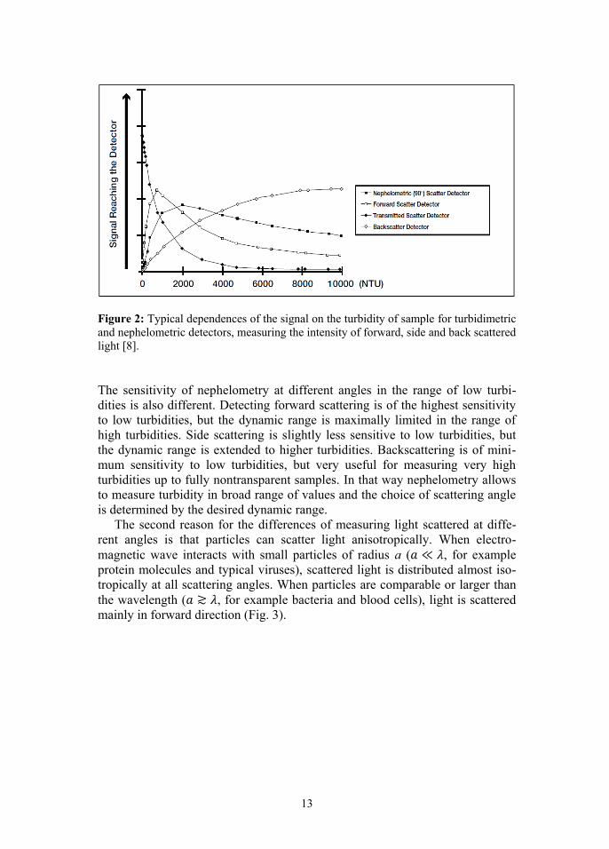
13

Figure 2: Typical dependences of the signal on the turbidity of sample for turbidimetric and nephelometric detectors, measuring the intensity of forward, side and back scattered light [ 8]. The sensitivity of nephelometry at different angles in the range of low turbi-dities is also different. Detecting forward scattering is of the highest sensitivity to low turbidities, but the dynamic range is maximally limited in the range of high turbidities. Side scattering is slightly less sensitive to low turbidities, but the dynamic range is extended to higher turbidities. Backscattering is of mini-mum sensitivity to low turbidities, but very useful for measuring very high turbidities up to fully nontransparent samples. In that way nephelometry allows to measure turbidity in broad range of values and the choice of scattering angle is determined by the desired dynamic range.

The second reason for the differences of measuring light scattered at diffe-rent angles is that particles can scatter light anisotropically. When electro-magnetic wave interacts with small particles of radius a ( , for example protein molecules and typical viruses), scattered light is distributed almost iso-tropically at all scattering angles. When particles are comparable or larger than the wavelength ( , for example bacteria and blood cells), light is scattered mainly in forward direction (Fig. 3).

14

Figure 3: Calculated polar diagrams of scattering (indicatrixes) on latex spheres in water with radii a from 0.1 to 1.6 μm. Every indicatrix is representing decimal loga-rithm of intensity of scattered light depending on the direction of scattering, scattering particle is located in origin of coordinates, λ=650 nm. For that reason, to detect large particles (e.g. bacteria) with maximal sensitivity one has to measure light scattered in forward direction. In case of the processes occurring with changing morphology of the particles, simultaneous detection of light scattered at different angles allow to achieve information about the chan-ges in size and shape of the particles [ 12].

In most of nephelometers side scattering is used for turbidity measurements. Although theoretically forward scattering is more sensitive to low turbidities, parasitic scattering and illumination from transmitted light beam are also con-centrated at small angles and are minimal at 90°. When detecting large particles (bacteria) with highest sensitivity forward scattering is used, but chosen scattering angle is rather high (typically 30°) to achieve optimal balance between the sensitivity and negative influence of stray light [ 13].

15

2.2. Dynamic light scattering In turbidimetry and nephelometry the output signal after the amplifier contains two components – constant and variable. Constant component is a function of the intensity of scattered light and considered as useful signal. Variable compo-nent is usually considered as noise and is ignored by signal averaging over the time of order of seconds. However, variable component can be also informative under special conditions. This approach is used in dynamic light scattering (DLS) method also called photon-correlation spectroscopy. In DLS, the changes of the intensity of scattered light in time are analyzed, but not the mean intensity. For the functioning of DLS, the use of coherent monochromatic light source (laser) is fundamentally significant. The cuvette with particles under in-vestigation in liquid is illuminated with light beam; the scattered light is thoroughly collimated and detected with sensitive photon-counting receiver (photomultiplier or avalanche diode). Since reference light beam is mono-chromatic and coherent, electromagnetic waves scattered by particles under in-vestigation interfere forming accidental interference pattern called speckle (Fig. 4).

Figure 4: Typical accidental interference speckle pattern.

16

Since scattering particles move, speckle pattern changes in time, fluctuate, and the mean intensity on the detector changes in time too. In DLS, the cuvette with particles under investigation in liquid is thoroughly thermostated. As a result, only Brownian motion defines the movement of particles. Free path of the particle in Brownian motion depends on its size monotonously; therefore, the frequency of speckle fluctuations on the detector is connected with particles size unambiguously. Analysis of fluctuations frequency of intensity on the detector allows to determine size distribution of the particles in the cuvette. Typical DLS analyzers has dynamic range from 1 nm to 6 μm. Despite being highly infor-mative, DLS has not being widely used in clinical laboratory practice because of high complexity and low throughput of corresponding analyzers.

2.3. Coherent fluctuation nephelometry

In coherent fluctuation nephelometry (CFN) the dynamic approach is also used and the fluctuations of the intensity on the detector are analyzed, at the same time CFN is oriented for turbidity measurements and is related to conventional nephelometry in that respect. In CFN laser is fundamentally used as a source of reference light beam to form speckle pattern on the detectors. Two detectors are installed symmetrically relatively to reference light beam. This setup allows to subtract mean nephelometry signals easily and effectively using differential amplifier (DA), detecting only variable component of nephelometric signal related to speckle fluctuations (Fig. 5).

Figure 5: The block diagram of coherent fluctuation nephelometry, – the intensity of reference light beam, – the intensity of light, scattered at angle , ADC – analog-to-digital converter, DA – differential amplifier.

17

Speckle pattern on the detectors is formed both by the light scattered by particles under investigation and by stray light from different parts of optical path of the device, first of all from the cuvette. Parasitic stray light is formed by immovable parts of the device, so parasitic speckle pattern is static and does not change in time. Static parasitic and useful fluctuating speckle patterns add together. When subtracting signals from two detectors by DA, static speckle is subtracted and resulting signal depends almost only on fluctuating part of speckle pattern formed by particles under investigation. Therefore, static stray light almost do not influence the measured signal allowing to reach high sen-sitivity to low concentration of particles under investigation.

Particles in liquid undergo Brownian motion. Typical frequency of speckle fluctuations for Brownian motion depends on particles size and scattering angle and is fractions of Hz for forward scattering by bacteria [ 14]. To shift the fre-quencies to higher range that is more convenient for detecting, flows in the liquid are made. Any stirrer can be used for that purpose, for example, magnetic stirrer, but the most technologically convenient stirring is convection. To pro-duce a convection, the heater is used firmly contacting the cuvette from the bottom, at the same time the upper put of the cuvette is not termostated. There-fore, the temperature gradient is created in the liquid resulting in the convective flow. Such convection is enough to shift the frequencies of fluctuations of speckle pattern, formed by forward scattering to hundreds of Hz in standard semimicro cuvette with 1 ml of liquid [ 15].

2.4. Elastic light scattering in clinical laboratory practice

Optical methods based turbidity measurement are widely used in laboratory practice, for example for drinking water and other liquids quality assessment [ 5]. In clinical laboratory practice, such methods are used to study the processes in colloids and suspensions that occurs with turbidity changes. Two most wide-spread processes are immunoagglutination reactions and growth of microorga-nisms.

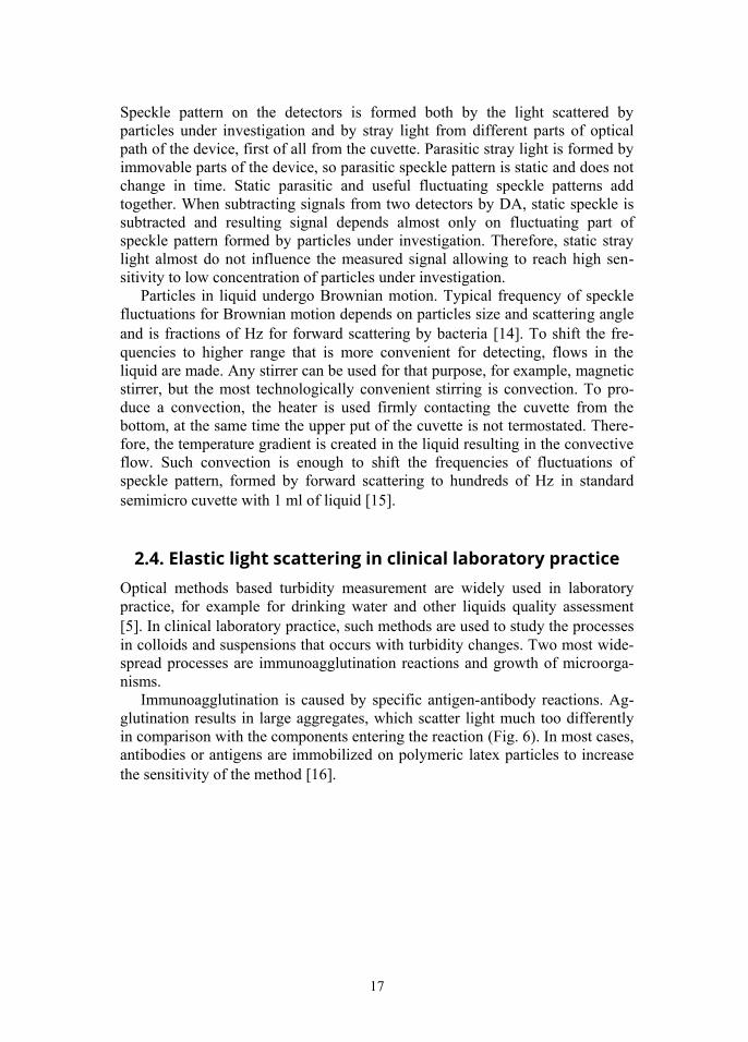
Immunoagglutination is caused by specific antigen-antibody reactions. Ag-glutination results in large aggregates, which scatter light much too differently in comparison with the components entering the reaction (Fig. 6). In most cases, antibodies or antigens are immobilized on polymeric latex particles to increase the sensitivity of the method [ 16].

18

Figure 6: A block diagram of latex immunoagglutination [ 16]. Antibody-antigen reaction results in massive aggregation of particles. When detecting growth of microorganisms, bacteria or fungi are incubated in nutrient broth; they divide and the increase of their number results in the in-crease in light scattering.

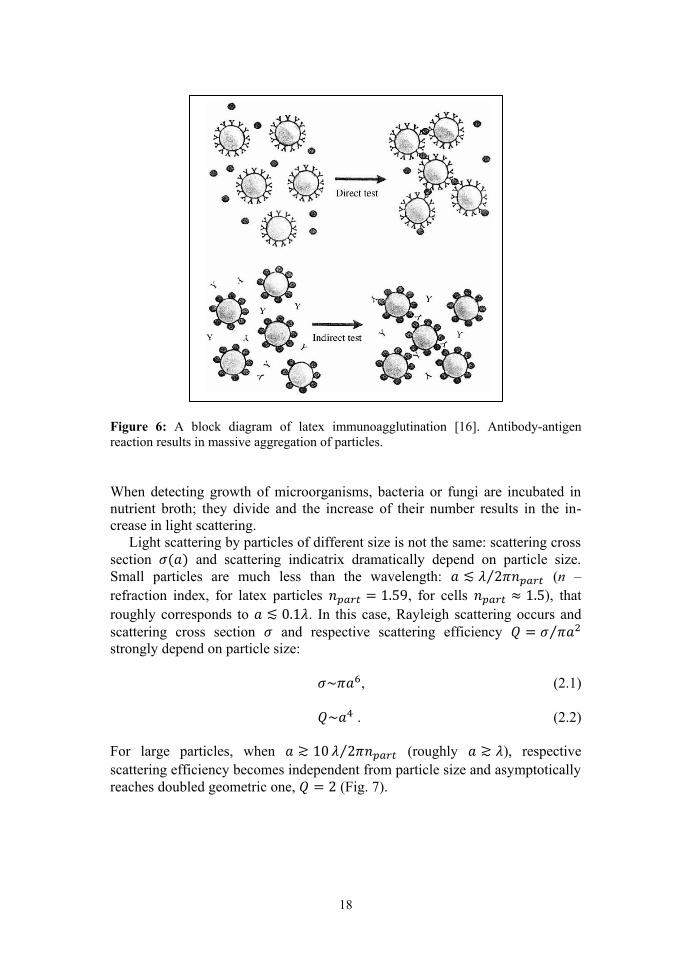
Light scattering by particles of different size is not the same: scattering cross section and scattering indicatrix dramatically depend on particle size. Small particles are much less than the wavelength: (n – refraction index, for latex particles , for cells ), that roughly corresponds to . In this case, Rayleigh scattering occurs and scattering cross section and respective scattering efficiency strongly depend on particle size:

, (2.1)

. (2.2)

For large particles, when (roughly ), respective scattering efficiency becomes independent from particle size and asymptotically reaches doubled geometric one, (Fig. 7).

19

Figure 7: Dependence curve of respective scattering efficiency on size parameter for Rayleigh scattering (dotted line) and Mie scattering (solid line) [ 17]. In range of small size when Rayleigh scattering occurs and strong dependence is observed . For large particles when respective scattering efficiency becomes independent from particle size and asymptotically reaches doubled geometric one . For recording immunoagglutination reactions, Rayleigh’s strong dependence of scattering cross section on particles size is used. For example, typical size of protein molecules and antibodies are roughly about 5 nm. When compact aggre-gate of 8 molecules is formed, its size doubles to approximately 10 nm. According (2.1), such aggregate will scatter times more light than single molecule.

For immunoagglutination reactions, latex particles are chosen of small size (with diameter of about 100 nm for wavelength 650 nm, i.e. ) to use strong dependence of scattering cross section on the size of forming aggregates. When aggregates are forming, their number decrease in comparison with number of particles initially entering the reaction. When particles with size

agglutinate into aggregates of size , their number decrease proportio-nally to the ration of their volumes:

. (2.3) Considering (2.1) the ratio of scattering cross sections of all particles:

.

20

Consequently, for small particles (Rayleigh’s scattering), cross section of aggre-gating particles is proportional to third power of the size of aggregates:

. (2.4) In case of detecting growth of microorganisms, when their turbidity increases due to cell division, effect is also achieved because of increase of particles size. Indeed, every new cells is built of peptide and protein molecules from the nutrient broth. Their size is very small (about 1 nm), and size of typical bacteria is about 1 μm, the difference in respective scattering efficiency is dramatically huge, so one can neglect the scattering on the components of nutrients broth and consider that light is scattered only by microorganisms.

In laboratory practice mainly turbidimetry and nephelometry based analyzers are used to record immunoagglutination reactions [ 16]. In case of turbidimetry, light beam passes through the cuvette where aggregation of particles occurs, the intensity of light decreases due to scattering and absorption of light by the particles in the liquid. The wavelength of reference light beam is chosen so that no components of biological liquid under investigation absorb light, so turbidity changes are caused mainly by changes in light scattering. Polymeric particles used in immunoagglutination reactions also do not absorb visible light.

In case of low-angle nephelometry, the increase of turbidity due to aggre-gation of particles is accumulated with the effect of anisotropy of light scat-tering by large particles. Larger the aggregates, more light is scattered in for-ward direction (Fig. 3).

In clinical microbiology optical methods are used to record growth curves of microorganisms [ 18], although in general automation of microbiology laborato-ries is still rather low and the manual techniques are still most common [ 19]. Turbidimetry allows to determine number of microorganisms at high concentra-tions, that’s why turbidimeters are widely used to prepare suspensions with high concentrations of cells according to McFarland turbidity scale. Turbidimetry also allows to record growth curves of microorganisms in the presence of anti-biotics (antibiotic susceptibility testing – AST). However, due to poor detection limit of bacteria, turbidimetry is not suitable for testing of biological liquids with low concentration of microorganisms.

For several sterile biology liquids such as blood and cerebrospinal liquid, presence of microorganisms in any concentration is pathologic, so the higher is the sensitivity of optical method, the less time is needed to detect microbial growth. Urine has the special place in clinical microbiology practice, since urinary tract infections are among the most actual infectious diseases and urine testing for bacteriuria is one of the most frequent analyses in microbiology laboratories [ 20]. Potential uropathogens in concentration 103 – 105 CFU/ml in urine sample is considered significant depending on sex, age and clinical picture of the patient [21], so high sensitive optical methods are required to detect microbes at such low concentrations.

21

Conventional microbiological techniques (culturing on solid nutrient media) needs 24-48 hours for urine screening and 24 hours for AST, that is too long. To increase the effectiveness of treatment the result should be obtained much faster. For that reason, development of new fast techniques is of great impor-tance.

Analyzers based on registration of changes in the intensity of scattered light over time resulted from microorganisms division, are used since 1980s for direct detection of viable microorganisms in urine samples [ 22]. Analyzers HB&L (Alifax S.r.l., Italy) and BacterioScan 216Dx (BacterioScan Inc., USA) allow not only to test urine samples rapidly, but also to determine antibiotic susceptibility of bacterial cultures [ 18, 23, 24]. For bacteriuria screening, urine samples are mixed with nutrient broth and growth delay time is analyzed within 3-4 hours. When bacteriuria is clinically significant, microflora in urine starts to grow quickly. When only contaminating microorganisms are present in urine, they need several hours for adaptation so growth is delayed [ 24].

To achieve high sensitivity in nephelometry, one must use cuvettes of high optical quality and construct analyzers with complicate optical scheme to reduce stray light. It complicates laboratory nephelometers, however they still lack sensitivity to estimate concentration of bacteria in urine in addition to growth curves recording. Information about the turbidity of urine samples would allow to evaluate concentration of microorganisms present, increasing diagnostic reliability of determining positive and negative urine samples.

Besides nephelometry, analyzers based on flow cytometry are used for urine screening in laboratory practice, for example UF-1000i (Sysmex Corporation). It combines cytofluorimetry and conductometry and can analyze concentration of microorganism in urine sample and composition of urine sediment. When bacteriuria is significant, the concentration of microorganisms in urine is higher in average, than in case of contamination. UF-1000i is used as an instrument for preliminary selection of urine samples for further culturing [ 25]. Despite the high sensitivity to the number of bacteria in urine, flow cytometry does not give information about their viability (does not analyze growth) that negatively influences its diagnostic effectiveness.

22

3. EXPERIMENTAL

3.1. CFN-analyzer early prototypes To investigate the basics of CFN method operating, two-channel CFN prototype of CFN-analyzer “CFN-2” was used (Medtechnopark Ltd., Russia). Standard photometric polystyrene semimicro type cuvettes with 1.6 ml volume (optical path 10 mm) were used with polyethylene stoppers (Vacutest Kima S.r.l., Italy). The first prototype of multichannel analyzer “CFN-48” (Medtechnopark Ltd., Russia) was used. It has mechanical positioning system for cuvettes. It allows to record the signal from the cuvettes consecutively using 6 CFN optical channels, one for standard 8-well strip of 96-well plate, each well with 200 μl of liquid. Each strip is moved back-forward perpendicular to the laser beam.

3.2. Calibration of CFN prototype To calibrate “CFN-2” prototype, latex polystyrene monodisperse spheres of radii 40, 60, 125, 200, 300, 390, 500 и 950 nm with initial mass concentration of 10% were used (“Diafarm” LLC, Russia). Formazine turbidity standard 4000 FTU (Sigma-Aldrich Co. LLC, USA) was also used. Dilution and other manipulations with standards were performed using distilled water and standard laboratory pipettes, disposable tips and test tubes of different volume.

3.3. Theoretical analysis of CFN method functioning To model the convection in the cuvette, ANSYS Fluent software 15.0 was used. Navier–Stokes equations were used to describe the processes occurring in the cuvette:

,

,

,

where – liquid density, – velocity components, – liquid pressure, – components of viscous stress tensor, – mass density of full energy, – internal energy, – components of heat flow vector. Viscous stress tensor takes the form:

23

,

where – viscosity of liquid.

Heat flow is described by Furrier’s law:

, where – specific thermal conduction of liquid.

Liquid density was considered to depend on temperature, table values were taken from [ 26], to calculate intermediate values linear interpolation was used. To describe process of heat transfer through the cuvette wall Newton-Richman law was used:

, where – normal component of heat flow, – the coefficient of heat transfer,

– external temperature, – temperature of the liquid near the wall. There are many methods to solve set of equations referred above. Main

classes of methods are finite-difference methods, finite elements methods and finite volumes methods. The latter naturally provides conservatism and are relatively simple to realize, so they were chosen to solve the problem.

The first step of this method is the partition of the volume under investi-gation for the cells. On the second step, the differential equations are integrated within the volume of the cell. The third step is the approximation of the flows on the borders of cells.

Consider a set of equation of the form:

,

in our case:

,

.

Integrating the differential equations, we have:

,

24

where is the vector . Let label the average value of vector in the cell with index :

. Suppose – the majority of numbers of all cells, that have joint border with cell , then

.

Approximation for boundary integrals (flows) are represented in the form

,

where – the area of the border between cells and , – quadrature weights, – approximations of normal flows in quadrature points .

At temperature 37˚С the density of water is . The viscosity of water is . The coefficient of heat transfer of all walls of the cuvette excluding the

upper one is .

The coefficient of heat transfer of the upper wall is .

3.4. Modeling of the processes underlying CFN Modeling of light scattering by particles in the cuvette, formation of speckle pattern on the detectors and CFN signal was made using Monte Carlo method in Maple 13 software. Indicatrixes and scattering cross sections of particles were calculated using Mie scattering theory for spheres of arbitrary size [ 27, p. 137–153]. In this theory, a rigorous solution of Maxwell’s equations for incident plane wave with linear polarization and corresponding boundary conditions on the surface of the sphere is obtained. Electric field on the distance from the sphere is represented by two components – parallel to the polarization of incident wave ( ) and perpendicular ( ):

,

,

25

where amplitude functions и are in the form of infinite series:

, (4.1)

, (4.2) where

,

,

,

,

where – associated Legendre polynomials, – complex refractive index of medium, size parameter – ratio of circumference of sphere to wavelength, , and – Ricatti-Bessel functions. Calculated indicatrixes were compared with ones, obtained using ScatLab software.

3.5. Agglutination of functionalized particles To study agglutination of functionalized particles, reagent kits “C-reactive pro-tein Novo” (Vector-Best LLC, Russia) and “MAP-Endotox spp.” (Rohat In-dustrial Scientific Company LLC, Russia) were used. Size of particles and their aggregates was determine by nanoparticles size analyzer based on DLS “АРН-2” (VNIIOFI, Russia). To study the influence of stirring with magnetic stirrer on aggregation reaction rate, aggregation analyzer “220LA” (Biola Ltd., Russia) was used.

3.6. Microbiology To study growth of microorganisms using CFN-analyzers, sugar meat-peptone and Mueller-Hinton broths were used (ООО “НИЦФ”, Russia). Antibiotics for susceptibility testing were obtained from the Department of new technologies, Pasteur Institute of Epidemiology and Microbiology (Russia).

26

4. GOALS OF THE STUDY

The main goal of the thesis was to investigate and optimize CFN method with aim to develop devices, oriented for wide use in laboratory practice. To achieve this, the following specific objectives were pursued: 1. To describe and model physical processes underlying CFN method. 2. To determine fields of application of CFN method. 3. To apply CFN method to registration of immunoagglutination reactions. 4. To optimize the parameters for developing prototypes of CFN-analyzer for

chosen field of application – clinical microbiology. 5. To study the effectiveness of developed microbiological CFN-analyzers

and to compare with other methods used in the field.

27

5. RESULTS AND DISCUSSION

5.1. Calibration of CFN prototype In prototype “CFN-2” the scattering light was detected at angle 6°–9°, the dis-tance between the cuvette and the detectors was 40 mm. Reference beam was produced by semiconductor laser with 1 mW power and geometrical size of light beam cross-section 1×2 mm2.

To investigate the features of signal dependence on concentrations of par-ticles of different size, calibration curves were obtained for latex polystyrene monodisperse spheres of radii 40, 60, 125, 200, 300, 390, 500 и 950 nm using prototype “CFN-2” (Fig. 8).

Figure 8: Calibration curves representing CFN signal dependence on mass con-centration of latex particles of different diameter in logarithmic coordinates. Formazine turbidity standard 4000 FTU was also used (Fig. 9).

5

50

500

1E-9 1E-8 1E-7 1E-6 1E-5 1E-4 1E-3 1E-2

CFN

sign

al, a

.u.

Mass concentration of latex particles

a = 40 nm а = 60 nm a = 125 nm a = 200 nma = 300 nm a = 390 nm a = 500 nm a = 950 nm

28

Figure 9: Calibration curves representing CFN signal dependence on turbidity of formazine standard. All calibration curves reach their maximum at high turbidities due to multiple light scattering.

5.2. Theoretical analysis of CFN functioning

5.2.1. Analysis of measurands in nephelometry and CFN

In CFN, nephelometric signals (light intensities) averaged by the area of the detectors are subtracted. Denote by the intensity in the point of detector j (j = 1, 2) at time moment t. Nephelometric signal on both detectors is value averaged by the area at given time moment. CFN signal is the difference between nephelometric signals

at given time moment. In nephelometry the measurand is the averaged signal over the time of order of seconds

(since both detectors are symmetrically located, nephelometric measurands are the same in average). In CFN, the measurand is root-mean-square of the difference between nephelometric signals over the time of the order of seconds:

. .

5

50

500

5000

0,01 0,1 1 10 100 1000

CFN

sign

al, a

.u.

FTU

29

Consider the averaged by the area of the detector intensity of scattered light as a variable random in time. Taking into account that random

variables and are independent and equally distributed since both detectors are symmetrically located, nephelometric signal is the mathematical expectation of random variable , and CFN signal is proportional to root-mean-square deviation of :

,

.

Since signal processing is made with finite digitizing rate and one measurement includes processing of signal at N time points, the relations can be expressed as:

,

, (5.0)

where N – quantity of time points in one measurement, k – time point number.

5.2.1.1. Nephelometric signal dependence on particles number and stray light

Let us determine the dependence of nephelometric and CFN signals on the number of particles in the cuvette N and the stray light from the optical path of the device. For that purpose, consider how speckle pattern forms on the detectors. For simplicity, we would consider interference of scattered light of one polarization on the point detectors.

Assume that N particles are in non-scattering liquid in the cuvette and they are illuminated by reference monochromatic coherent light beam. Every particle scatters light as the point source of electromagnetic radiation, so according to superposition principle N scattered waves interfere on the detector:

, where I – intensity of scattered light on the point detector, E – electric field strength on the detector, – phase shift for particle j, – initial phase of light for particle j, – frequency of electromagnetic radiation.

Consider the case, when all particles are equal, then , and the relation takes the form:

30

. For the scattered light of one polarization, we have:

. After squaring the sum, the equation is:

. (5.1) When particles in the cuvette move fast and chaotically, phase can be treated as a random variable, and the intensity of light on the detector, resulted from scattering by one of the equal particles, is defined by relation:

. (5.2) Let us find the mathematical expectation , corresponding to total nephelo-metric signal on the detector, averaged in time:

. Since random variables are independent and equally distributed, than the relation takes the form:

, or considering (5.2):

. Random variable is centralized, so:

, (5.3) and the mathematical expectation of intensity of scattered light on the detector is:

. (5.4) Consequently, the average light intensity on the detector from N equal particles is N times greater than from one particle. This result agrees with observed in practice – nephelometric signal is proportional to the number of scattering particles (in absence of parasitic stray light):

31

. (5.5) In the case when light scattered by particles is summarized with static stray light from optical path of the device with intensity , the equation for the intensity on the point detector takes form:

, After squaring the sum, we obtain:

. (5.6)

Considering (5.2), the mathematical expectation of intensity of scattered light on the detector is:

, The last term vanishes according to (5.3), so we obtain in nephelometry, that intensity of stray light is summarized with intensity of scattered light

:

. (5.7)

In CFN, the measurand is root-mean-square of the difference between inten-sities of scattered light on the detectors, so we consider the dispersion of light intensity on the detector. From (5.1) we have:

, or

. Dispersion of two independent random variables X and Y can be converted according the formula:

,

5.2.1.2. CFN signal dependence on particles number and

stray light

32

whence:

.

The dispersion of scattered light intensity from one of the equal particles, is defined by relation:

. (5.8) Considering (5.3) and (5.8) the dispersion of scattered light intensity is:

,

.

Thus, we have more complicated dependence of CFN signal on number of scattering particles N in comparison with nephelometry:

, (5.9) where k1 and k2 are constants.

The dependence is not linear, it is stronger than and weaker than , however the most important is that the signal monotonously increases with particles number increasing.

From Fig. 8 and Fig. 9 one can see, that calibration curves have maximum inclination it the range from to . The dependence is weaker for low concentrations of particles and stronger for high concentration for every calibration curve. All these findings agree with obtained relation (5.9).

In the case when light scattered by particles is summarized with static stray light from optical path with intensity of the device, the equation for the intensity on the point detector (5.6) takes form:

.

Since we have:

,

33

or

, (5.10)

where k1, k2 and k3 are constants.

The comparison of relations for dependences of signal on particles number (5.7) and (5.10) allow to conclude, that the parasitic stray light influences the signal in nephelometry and CFN in different ways. In nephelometry the sensitivity limit is bounded by the intensity of stray light:

.

In CFN the intensity of parasitic stray light does not bound the sensitivity limit (in the range of intensities, when the saturation of the detector does not occur), but influence the behavior of the dependence of the signal on particles number

. Stray light makes this dependence weaker.

5.2.2. Dependence of speckle fluctuations frequency on the direction of particles movement for forward scattering.

Consider how the direction of motion of scattering particles influences the frequency of speckle fluctuations. Let a couple of detectors are located in point C at a distance L from the scattering particle (point A). Reference light beam is directed along the main optical axis AB, the scattering occurs at the angle to the reference beam. The distances are , ,

(Fig. 10).

Figure 10: A block diagram for calculation of phase shifts in cases when particle moves in parallel or perpendicular to main optical axis. Consider two possible movements of the particle over time : in parallel or perpendicular to main optical axis. The dependence of speckle fluctuations frequency on the velocity of the particle is defined by the coefficient in the

34

ralation , where – phase shift caused by movement of the particle by distance over time .

Phase in the electromagnetic wave equation scattered by particle j is defined as:

,

where is wavelength of light. When the particle moves perpendicular main optical axis by distance , using Pythagorean theorem, phase shift takes the form:

,

. Since then vanishes because of its smallness, we approximate the root using Taylor series, and after cancellation we have:

, (5.11) To derive phase shift for movement of the particle along main optical axis, we notice then the wavelength scattered on the particle gains additional phase shift when particles moves in the direction of incident light beam. Considering this the equation for phase shift takes the form:

,

. Since then vanishes because of its smallness, we approximate the root using Taylor series, and after cancellation we have:

. (5.12) For small angles after approximating using Taylor series from (5.11) and (5.12) we have:

,

.

35

Consequently, for forward scattering:

.

Therefore, particle movement perpendicular to main optical axis leads to greater phase shift than movement along the main optical axis. That is why the stirring in the cuvette must be created perpendicular to the incident light beam. Just so, the convection flow is formed in the cuvette when it is heated from the bottom.

5.2.3. Modeling and experimental verification of

the convection in the cuvette

It has been found experimentally, that when heating standard photometric semi-micro cuvette with 1 ml of liquid from the bottom to 37˚С at normal room temperature 23±3°C, the temperature in the coldest upper part of the liquid is about 35˚С. When we use a probe, that is a relatively large particle visible by eye, put it into the cuvette and observe its movement in convective flows, we can roughly estimate the maximum convection speed as 1 mm/s.

To model convection in the cuvette using ANSYS Fluent software, three configurations of the heater were used. Configuration 1 – the heater contacts only with the bottom of one side wall of the cuvette, contact area is 100 mm2. Configuration 2 – heater contacts with the bottom of one side wall of the cuvette and with the bottom of the cuvette, contact area is 140 mm2. Con-figuration 3 – nonsymmetrical U-type heater contacts with the bottom of the cuvette and with both side walls, contact area is 190 mm2. The temperature of the heater is 37˚С, temperature of cuvette walls above the heater was 34˚С, 35˚С or 36˚С. Evaporation from the surface of the liquid (meniscus) was disregarded.

There were boundary conditions of non-leakage on all cuvette walls. Be-sides, the tangent component of liquid velocity was equal zero near all walls except the meniscus.

On Fig. 11 distributions of temperatures and velocities of convective flows in the cuvette are given for one of the calculated configurations.

36

Figure 11: Distributions of temperatures and velocities of convective flows in the cuvette for one of the calculated configurations (U-type heater, temperature of the walls 35˚С). Average and maximal velocities of liquid flows are given for different tempe-ratures of cuvette walls and configurations of heater in table 1. One can assess Reynolds numbers for obtained flows by maximal flow velocity using equation:

,

where is characteristic size of the cuvette (10 mm).

37

Table 1: Average (Vaver) and maximal (VMAX) velocities of liquid flows and Reynolds numbers depending on temperatures of cuvette walls and configuration of heater

Temperature of cuvette walls, ˚С

Heater configuration VMAX, mm/s Vaver, mm/s Re

34 1 0.98 0.11 14 34 2 1.55 0.39 22 34 3 1.08 0.4 15 35 1 0.61 0.061 9 35 2 1.18 0.31 17 35 3 0.79 0.3 11 36 1 0.16 0.014 2 36 2 0.62 0.17 9 36 3 0.43 0.17 6

In model built, stable convective flow develop within 1 minute after virtual installing of the cuvette onto the heater. In “CFN-2” prototype, it also takes about 1 minute for convection to develop.

At temperature 35˚С of the cuvette walls, temperature difference between liquid in upper and lower parts of the cuvette is 2˚С, which corresponds to the observed in experiment. At configuration of the heater 3 (which corresponds to “CFN-2” prototype), the maximal calculated flow speed was about 0.8 mm/s that is in good agreement with the experimental value of 1 mm/s.

All calculated convective flows are characterized with low Reynolds numbers from 2 to 22, much less than critical number [ 28]. Con-sequently, convective flows in the cuvette are always laminar.

Convective flows of maximal velocities are achieved when using configu-ration 2, although contact area with the heater is greater at heater configuration 3.

5.2.4. Doppler effect impact on speckle fluctuations frequency

When summating the electromagnetic waves scattered by particles, phase of particle j can vary in time not only due to changes in position of

particle relatively to detector , but also due to the changes of wave vector . Modulus of wave vector depends on the wavelength of reference light beam:

,

where – the frequency of incident light. Since particles move relative to reference light beam, the frequency of light

changes due to Doppler effect. When particles move perpendicular or along reference light beam the equations for the frequency are:

38

,

,

where – the ratio of particle velocity to the speed of light. For convective stirring , and upper estimate is . Due to smallness of the expressions for frequency shifts take the form:

,

.

Maximal frequency shift is caused by particle shift along the reference light beam. Corresponding phase shift due to frequency shift is:

.

For and phase shift caused by Doppler effect is much less than (phase shift causing the maximal change the amplitude of the wave):

. Consequently, Doppler effect do not contribute to speckle pattern fluctuations in CFN method.

5.3. Modeling the processes underlying CFN method

5.3.1. Modeling the scattering indicatrix and cross section of single particle

To consider anisotropy of light scattering by particles, indicatrix of light was modeled using Mie scattering theory for spheres of arbitrary size. For this purpose amplitude functions were calculated according to (4.1, 4.2) and the following relation for dependence of intensity of light scattered at angle was used:

.

Amplitude functions are given by infinite series that are convergent, and the convergence rate is the weaker the larger are the particles. By default calculations are made with accuracy until tenth decimal place in Maple 13, therefore infinite series were calculated with nearly the same accuracy. The

39

summation was interrupted when the next term of the sum was less modulo than 10-10 of the sum of previous terms. The curve represented the number of terms needed for different particles sizes is represented on Fig. 12.

Figure 12: The dependence of number of terms in infinite series on particle radius a, to achieve calculation accuracy 10-10. On Fig. 3 calculated indicatrixes for particles of different size are given. Indicatrixes agree with those obtained using ScatLab Software.

5.3.1.1. The dependence of particle scattering cross section on radius

Besides the angular distribution of scattered light, Mie theory allows to calcu-late scattering cross section of the particle depending on its size. The equation for respective scattering efficiency is of the form:

.

The curve representing dependence of calculated respective scattering effi-ciency on particle radius is shown on Fig. 13. for small particles ( ) and for large particles ( ). Calculated dependence agrees with theoretical one shown on Fig. 7.

01020304050607080

0 1 2 3 4 5 6 7

Num

ber o

f ter

ms i

n se

ries

a, μm

40

Figure 13: The dependence of calculated respective scattering efficiency on particle radius in logarithmic coordinates. Refractive index of particles (polystyrene latex), refractive index of medium (water).

5.3.1.2. The dependence of scattering cross section on radius for suspension of particles with fixed concentration

During the processes of aggregation/desegregation of particles, the concentra-tion of matter do not change in time, and when the size of particles changes, their number also changes. Let us fix volume concentration of particles:

. Consider monodisperse particles for simplicity. Consider the intensity of light , scattered by the suspension of the particles at angle . In this case, the intensity of scattered light is determined by total scattering cross section of particles and by scattering indicatrix. Let

is part of light scattered by particle of radius a at angle into elementary solid angle, it is determined by scattering indicatrix. Therefore, we have:

.

Since for small particles ( ):

, ,

, then . Calculated dependences of intensity of light, scattered at diffe-rent angles , on radius for the suspension of monodisperse spheres with fix volume concentration of matter are given on Fig. 14. Reference curve is the dependence of total cross section of all particles on radius, ignoring the aniso-tropy of scattering (it represents virtual particles scattering light to all angles anisotropically, for such particles scattered light intensity depends only on cross section).

1E-9

1E-7

1E-5

1E-3

1E-1

1E+1

1 10 100 1000 10000 100000

Q, a

.u.

a, nm

41

Figure 14: Calculated dependences of light intensity scattered at different angles

, on radius of particles. Suspension consists of monodisperse spheres and their volume concentration is fixed ( , when particles size changes, their number also changes. For particles of small radius the intensity of scattered light is almost independent on the scattering angle and is determined only by scattering cross section. Starting from the dependence of total cross section deviates from the dependence . The intensities of light scattered to different angles also have the different behavior starting from due to lengthening of indicatrix in the forward direction (Fig. 3). For lower scattering angles strong dependence preserves for larger particles size during the aggregation process. For side and backscattering the effect is opposite – indicatrix decreases at chosen angle and the dependence deviates from

earlier and steeper than the dependence of total scattering cross section.

5.3.1.3. Multiple scattering influence on the dynamic range upper limit

For turbidity measurements both in conventional nephelometry and in CFN, the dynamic range has upper limit due to multiple scattering. At low turbidities, light scattered by every particle in liquid reaches the detector without second scattering on other particles with probability close to 100%. When number of particles increases, there finally occurs the situation when scattered light cannot reach the detector without scattering on second particle. At so high con-

1E+05

1E+07

1E+09

1E+11

1E+13

1E+15

1 10 100 1000 10000

Inte

nsity

of s

catte

red

light

, a.u

.

Radius of scattering particles a, nm

Total cross section of all particles Scattering intesity to 2-3 degreesScattering intesity to 4-6 degrees Scattering intesity to 9-11 degreesScattering intesity to 38-52 degrees Scattering intesity to 80-100 degreesScattering intesity to 128-142 degrees

42

centration, inverse dependence of the signal on particles number is observed (Fig. 8). Let us estimate the critical concentration when multiple scattering becomes significant and study its dependence on particle size.

Consider for simplicity the suspension of monodisperse spheres of radius a in non-scattering liquid in the cuvette. Let is number concentration of particles and is volume concentration; they are related by the equation:

,

Let is the optical path in the cuvette and is the the cross sectional area of reference light beam. Illuminated volume of suspension inside the cuvette is

. Multiple scattering starts to influence the signal when the total cross section of the particles becomes comparable to the cross sectional area of light beam:

,

where is coefficient of order of unity, is scattering cross section of particle j. Since all particles are equal then (where Q is respective scattering efficiency of particle), we have:

.

Since :

.

Expressing via the volume concentration we obtain:

.

To characterize the relationship between turbidity of the liquid and the optical path in the cuvette, the value of free path of light is used, which is estimated as:

.

When path length of light becomes comparable to liner dimensions of the cuvette, multiple scattering becomes significant.

To calculate critical concentration of particles, dependence is used (Fig. 13).

On Fig. 15 one can compare calculated dependence of critical concentration on particles radius (for ) with experimentally determined maximums of

43

dependences of signal on concentration for monodisperse latex spheres in water from Fig. 8 (refractive index of particles , refractive index of medium

wavelength ).

Figure 15: Calculated (orange) and experimental (blue) dependences of critical con-centration on particles radius. Since for small particles ( ) we have:

,

and for large particles ( :

.

Experimental dependence of critical concentration on particle size is in good agreement with calculated curve.

5.3.2. Speckle pattern modeling on the detectors

To model the accidental speckle pattern on the detector, the following geometry of CFN device was chosen. Cuvette H×W×D = 25×4×10 mm3 (standard semi-micro). Reference light beam with circular cross section of 2 mm diameter passes through the symmetry axis of the cuvette. The distance between the plane of detectors and center of the cuvette along the light beam is 25 mm. The distance between the detectors is 1 mm. The average scattering angle is 7˚; range of scattering angles is 4.1˚–11.7˚. Linear dimensions of the detectors vary

0,00001

0,0001

0,001

0,01

0,1

10 100 1000 10000

Crit

ical

vol

ume

conc

entra

tion

of p

artic

les

Particles radius a, nm

44

in different calculations and is specified separately. The view on the optical elements of the device in the direction of light beam is shown on Fig. 16.

Figure 16: The view on the optical elements of CFN device in the direction of light beam. On Fig. 17 calculated speckle pattern in detector zone is shown. To obtain it, 50 scattering particles of radius were randomly placed in part of the cuvette illuminated by incident light, which corresponds to the concentration of particles about 1600 pcs/ml. The detector area was chosen 50×50 μm2, it was divided into 104 elementary areas, and intensity of light scattered by particles was calculated on every elementary area. Wavelength of incident light

.

25 3

12.5

4

Detectors

Reference light beam

Cuvette

1

Main optical axis

45

Figure 17: The example of calculated speckle pattern in the detectors zone. To estimate size of speckle grain, simple two-dimensional correlation function

was built. Point n of correlation function is defined by relation:

, where is the calculated speckle intensity on elementary area and is normalization factor equal to total number of terms in the sum. Such correlation function allows to estimate speckle correlation distance which corresponds to average distance from the center of speckle grain to the point where the inten-sity of light reduces e times. Speckle correlation distance depends on the wavelength, the radius of incident light beam and the distance from scattering particles to the plane of the detectors [ 29]:

. (5.13) For chosen parameters we obtain:

.

On Fig. 18 two-dimensional correlation function is shown for detector area 1000×1000 μm2, divided into 2.5×105 elementary areas. It allows to estimate speckle correlation distance as 7-8 μm, which roughly agrees with theoretical value.

46

Figure 18: Two-dimensional correlation function for calculated speckle pattern. X axis represents distance of correlation (division value is 2 μm), Y axis represents the power of correlation in a.u. Speckle grain size is estimated as doubled speckle correlation distance and is about 15 μm in our model.

Based on speckle correlation distance, we will use the fineness of sub-division of detector area on elementary areas 2×2 μm2 in further modeling.

In built model, the influence of the number of scattered particles on corre-lation distance was studied ( that corresponds to con-centrations from 2.5×102 to 3.3×104 pcs/ml). In addition, the influence of particles radius in range from 0.05 to 3 μm was studied. Both parameters did not influence on speckle correlation distance, which agrees with (5.13). So particles number and size do not influence speckle grain size. 5.3.3. Modeling of root-mean-square deviation of the difference

between average intensities on the detectors

To model the differential signal, particles were put into illuminated part of the cuvette randomly 30 times in series. The area of the detector was chosen 40×40 μm2, each detector was divided into 400 elementary areas, and the intensity of scattered light was calculated on every elementary area. The dependences of mean intensities and the difference of intensities on number of calculation are shown on Fig. 19.

47

Figure 19: Mean intensities on the detectors (red curves) and the difference of intensities (blue curve) depending on number of 30 random calculation. The next step was to model the behavior of differential signal on particles number. In CFN, the signal is root-mean-square deviation of the difference between intensities on the detectors according (5.0). The dependence of calculated signal on number of scattering particles for radius is shown on Fig. 20.

Figure 20: The dependence of calculated CFN signal on number of scattering particles for particles radius in logarithmic coordinates, calculation is made 4 times. The dependence on particles number is close to linear and approximately

, which is in good agreement with theoretical result according to (5.9).

1E+0

1E+1

1E+2

10 100 1000

CFN

signa

l, a.

u.

Number of scattering particles

Calculation 1 Calculation 2 Calculation 3 Calculation 4

48

5.3.4. Influence of constant stray light on CFN signal

To model the influence of stray light, two models were used – uniform parasitic illumination of the detectors and illumination by parasitic speckle. The intensity of uniform illumination was chosen to exceed the intensity of light scattered by one particle, 50, 100 and 200 times. To create parasitic speckle on the detectors nonmoving virtual particles were placed into the cuvette and scattered incident light. All particles parameters were the same as the particles under investi-gation, the number of virtual particles were 50, 100 and 200.

The modeling was performed for particles of radius 1.25 μm at the same conditions as in chapter 5.3.3. The curves representing dependence of CFN signal on particles number for uniform parasitic illumination with different intensity is shown on Fig. 21.

Figure 21: The curves representing dependence of CFN signal on particles number for uniform parasitic illumination with different intensity.

The curves representing dependence of CFN signal on particles number for illumination by parasitic speckle with different intensity is shown on Fig. 22.

1E+0

1E+1

1E+2

10 100 1000

CFN

sign

al, a

.u.


Without parasitic stray light Parasitic stray light x50Parasitic stray light x100 Parasitic stray light x200

49

Figure 22: The curves representing dependence of CFN signal on particles number for illumination by parasitic speckle with different intensity. Consequently, uniform parasitic illumination of the detectors do not influence the CFN signal at all. Illumination with parasitic stationary speckle makes the dependence of the signal on particles number weaker that is in good agreement with theoretical result according to (5.10), since the more is intensity of stray light , the weaker is the dependence .

5.3.5. The dependence of speckle fluctuations frequency on particles velocities

To model the frequency spectrum of CFN signal and to compare with real spectrum obtained by “CFN-2” prototype, particles were moved step-by-step to obtain the evolution of signal in time. For that, particles of radius 1.25 μm were placed into the cuvette (in average 19 particles were illuminated by light beam every move), these particles formed the speckle pattern on the detectors. The initial positions of the particles were set randomly. Then the particles moved along the longest wall of the cuvette in one direction, and the velocity near the wall was minimal and maximal in the center of the cuvette. For that, the distribution of particles velocities corresponded the sinusoid (Fig. 23).

1E+0

1E+1

1E+2

10 100 1000

CFN

sign

al, a

.u.


Without parasitic stray light Parasitic stray light x50Parasitic stray light x100 Parasitic stray light x200

50

Figure 23: A schematic of particles movement in the simplest model of flow cuvette. When the particle reaches the upper plane of the cuvette, it is moved to the lower plane of the cuvette into the same position on the plane. Therefore, the simplest model of flow cuvette was created. One measurement was made within one second with 1023 consecutive particles movements to achieve 1024 time points. Signal obtained was converted with fast Fourier transform to achieve the frequency spectra. The measurement was made five time, obtained Fourier spectra were averaged.

To compare the results of modeling with experimental data, the standard cuvette was replaced with optically transparent pipe of 5×5 mm2 inner section in “CFN-2” prototype. The flow in the pipe was organized with constant velocity by means of perfusion pump.

Typical dependencies of signal on time, obtained by modeling and experi-ments, are shown on Fig. 24.

Cuvette in two projections

Reference light beam

Profile of particles velocities

51

Figure 24: Typical dependencies of signal in a.u on time, obtained by modeling (red) and experiments (blue) using “CFN-2” prototype. Typical Fourier spectra obtained by modeling and experiments are shown on Fig. 25.

Figure 25: Typical Fourier spectra obtained by modeling (red) and experiments (blue), X axis represents the frequency of signal fluctuation in Hz, Y axis represents Fourier amplitude in a.u. (logarithmic scale).

52

The shapes of modeled and experimental Fourier spectra are similar. The difference is that in CFN-prototype the bandpass has lower limit of about 10–20 Hz, so low frequencies are cut off.

Fourier spectra obtained can be characterized by width. It is defined by fre-quencies of speckle pattern fluctuations, which in turn are defined by velocities of moving particles in liquid. To determine the dependence of frequency spectrum width on the velocity of particles, the model of flow capillary was used. Experimental and calculated Fourier spectra width depending on flow velocity are shown on Fig. 26.

Figure 26: The dependence of typical Fourier spectra width on flow velocity for suspension of latex particles of 1.25 μm diameter, obtained by calculation and in experiment. The dependencies are similar. The differences are apparently related with the simplicity of the model used for calculation.

5.3.6. The influence of the bandpass of electronics on the dependence of CFN signal on particles velocities

The signal in CFN is root-mean-square of the difference between mean inten-sities on the detectors (5.0):

.

By Parseval’s theorem, the signal can be expressed as root-mean-square of Fourier spectrum components:

10

100

1000

0,02 0,2 2Four

ier s

pect

rum

wid

th, H

z

Flow velocity, mm/s

Experimental Calculated

53

, (5.11)

where is the component k of discrete Fourier transform of signal

. Consequently, the signal is the area under the curve on Fourier spectra graph.

Every electronics for variable signal processing is characterized by the band-pass. Frequency spectra lower cutoff can be seen on Fig. 25 when comparing experimental and calculated Fourier spectra. Due to cutoff, the first several Fourier components do not contribute to the signal (5.11). Let us look at speci-fic examples, how cutoff influences the signal in “CFN-“2 prototype.

Stirring of liquid in the cuvette is caused by convection in “CFN-2” proto-type. The movement of scattering particles causes broadening of signal Fourier spectra, as the result it can be detected easily. For example, convection in stan-dard semimicro cuvette heated at 37°C is characterized by the velocities of particles about 1 mm/s, and the width of Fourier spectra is in the range from 500 to 1000 Hz depending of scattering angle. In “CFN-2” prototype ADC is characterized by upper cutoff of tens of KHz. Specialized ADC as usual have higher upper cutoff, but most of ADC have the similar lower cutoff of several Hz or tens of Hz. Since CFN signal frequencies do not exceed several KHz, the upper cutoff of ADC does not influence the signal. For that reason, let us study the influence of lower cutoff on the dependence of CFN signal on particles velocities.

It was found experimentally, that when the velocities of particles in the cuvette increase, the Fourier spectrum width also increases, at the same time the amplitude of the Fourier components decreases (Fig. 27).

Figure 27: The example of the increase of Fourier spectrum width and the decrease of the amplitude of Fourier components caused by the increase of the velocities of particles in the cuvette (left graph – low velocities, right graph – high velocities). X axis represents frequency in Hz; Y axis represents amplitude in a.u. in logarithmic scale.

54

Let us study experimentally the dependence of CFN signal on velocity of the flow through the pipe described in chapter 5.3.5 for suspension of latex particles of 1.25 μm diameter. The result is shown on Fig. 28.

Figure 28: The dependence of CFN signal on average velocity of the flow through the capillary for suspension of latex particles of 1.25 μm diameter in logarithmic coordinates. For the velocities less than 0.02 mm/s the signal is minimal and does not depend on the velocity. If we extrapolate the curve on Fig. 26, we obtain, that velocity 0.02 mm/s corresponds to Fourier spectrum width of about 15–20 Hz. It is consistent to lower cutoff for “CFN-2” prototype (10–20 Hz), which can be seen on Fig. 27. Therefore, for velocities less than 0.02 mm/s all useful signal is out of the bandpass.

For the velocities greater than 0.5-0.7 mm/s the signal reaches its maximal value and practically does not depend on the velocity. It means, that almost all useful signal is shifted to higher frequencies and lower cutoff cuts only insigni-ficant part of the signal.

Let us study experimentally the dependence of CFN signal on the velocity of convective stirring in standard semimicro cuvette for the suspension of latex particles of 1.25 μm diameter. For this, we compare Fourier spectra of the signals obtained from six cuvettes, containing 500–1000 μl of particles suspen-sion (the cuvettes were put into “CFN-2” prototype one by one). For different volumes of suspension in the cuvette, the height of liquid column is from 12.5 to 25 mm. Since the dependence of the velocity of free convection on liquid column height is defined as [ 28], then the larger is the volume of liquid, the broader is the Fourier spectrum of CFN signal and the less is components amplitude (Fig. 29).

100

1000

10000

0,005 0,05 0,5 5

CFN

sign

al, a

.u.

Average particles velocities, mm/c

55

Fig. 29 confirms the straight relationship between Fourier spectrum width and the velocity of stirring. At the same time, the CFN signal is almost the same and does not depend on the volume of the liquid in the cuvette. Convective stirring provides enough velocities of particles’ movement to make CFN-analyzer operate in the regime, when the signal does not depend on velocities of the stirring. Minor perturbations in convective flows and changes in the volume of the liquid do not influence the signal significantly. This provides the stability of measurements using CFN-analyzer.

Figure 29: Pseudo-3D graph, representing the dependence of Fourier spectra width of CFN signal for the cuvettes with 500–1000 μl of particles suspension (1.25 μm dia-meter). X axis represents time in seconds, Y axis – frequency in Hz, colour indicates the amplitude of Fourier components in logarithmic scale (ascending amplitude: black-blue-white).

5.4. CFN application for detection of immunoagglutination reactions

Typical size of the particles in aggregation processes can be significantly diffe-rent from tens of nanometers to micrometers; also their concentration can vary considerably. Reagents kits based on immunoagglutination reactions can be divided into two classes by the type of results detection. The first class is the kits designed for instrumental detection of turbidity changes. Such kits are discussed in chapter 2.4. They are based on particles significantly less than the wavelength of light ( ), which provides strong increase of the turbidity during the aggregation of particles. The second class of kits is designed for visual observation of the results of particles aggregation: it is made semi-quantitatively by observing small/large clumps and lightening of the suspension that initially looks milky. For aggregation assessment, the scale from 1 to 4 is usually used. 1 means no aggregation, when particles suspension looks milky without clumps. 4 means very strong aggregation, when particles suspension looks like large clumps in transparent liquid Fig. 30).

500 μl 600 μl 700 μl 800 μl 900 μl 1000 μl

56

Figure 30: The picture of the results of latex agglutination reaction, numbers correspond to the agglutination strength [ 30]. The tiniest pattern that can be distinguished by naked human eye is about 120 lines per angular degree, that is about 50 μm at the distance of best vision of about 25 cm [ 16]. To achieve such big aggregates, large particles must be used of size . Historically the first immunoagglutination test using polymeric particles was designed for visual observation [ 31]. The advantage of such test is its simplicity: no specialized equipment is needed, besides the synthesis of latex particles of large size was technically more simple for a long time. The obvious disadvantages of visual agglutination test are semiquantative result and the complexity of automation.

Consider scattering cross section for the suspension of monodisperse latex particles of fixed mass concentration, which aggregate staying monodisperse. Size, number and scattering cross section of particles changes with time during aggregation. The dependence of total cross section on aggregates size is shown on Fig. 31.

When using turbidimetry, detection of aggregation is determined only by changes in total cross section of particles. For small particles strong dependence occurs, which is used in immunoturbidimetric diagnostic kits. Twofold increase of particles size is enough to detect reliably the 8-fold in-crease of the signal. For large particles weak dependence occurs, aggregation causes the lightening of the suspension, but relatively in-efficient.

In this chapter, CFN-analyzer is used for registration of aggregation of particles both of small and large size.

1 3

4

2

57

Figure 31: Calculated dependence of total scattering cross section of monodisperse particles on their radius , arrows show the ranges of particles size suitable for instru-mental (red) and visual (green) detection.

5.4.1. Detection of small particles aggregation using CFN-analyzer

Immuturbidimetric reagents kit “C-reactive protein Novo” (Vector-Best LLC, Russia) was used. It is designed for carrying out agglutination reaction in standard photometric semimicro cuvette using any laboratory turbidimeter with wavelength 540 nm and do not suggest to stir the liquid in the cuvette. 1 ml of latex suspension is put into the cuvette, then 7 μl of human blood serum under investigation is added and the kinetics of particles aggregation is detected using turbidimeter in two fixed time points – 10 and 120 seconds.

The suspension of functionalized latex particles were placed into the cuvet-tes in CFN-analyzer and particles size analyzer “АРН-2”. The reaction was carried out at 37˚С. Aggregation curves are shown on Fig. 32.

The comparison of the curves obtained by two methods allows to estimate the dependence of CFN signal on particles size. When the size of aggregates reaches , the dependence begins to weaken, and starting from

it saturates. Such dependence corresponds to scattering angle of about 8 degrees according to calculated curves on Fig. 14, which agrees with geometry of “CFN-2” prototype.

The reagents kit is optimized for turbidimetric registration, for that reason the initial turbidity of particles suspension is relatively high. For such reagents kits CFN-analyzer has no advantage over standard laboratory turbidimeters, since its high sensitivity is not used. The analyzer of specific proteins in human serum “BN ProSpec” (Siemens Healthcare GmbH) is known to use nephelo-metry to detect the aggregation of functionalized particles. It is used with

1E+0

1E+1

1E+2

1E+3

1E+4

1E+5

1E+6

1E+7

0,001 0,01 0,1 1 10 100

Tota

l sca

tterin

g cr

oss s

ectio

n Σ,

a.u.

Particle radius a, μm

58

specialized reagents kits, optimized for nephelometry. Due to higher sensitivity in comparison with turbidimetry, the analyzer allows to reduce the consumption of antibodies, which are the most expensive part of the reagents kits, thereby reducing the cost of the analysis.

Figure 32: Aggregation curves of functionalized particles “C-reactive protein Novo” obtained by CFN-analyzer and particles size analyzer “АРН-2”; at time 0 the calibrator with concentration 57 μg/ml was added. The feature of small particles ( ) aggregation processes is the indepen-dence of reaction rate on stirring. Particles diffusion provides high rate of collisions of particles that is not significantly increased by additional stirring. This observation is confirmed by independence of reaction rate on stirring velocity. Moreover, in DLS method uniform thermostating of the cuvette is provided to exclude convection completely, and the reaction rate is the same as with convective stirring. One can notice that on late stage of the reaction the size of aggregates measured by “АРН-2” significantly fluctuates. It is due to large aggregates move slowly without stirring and are distributed unevenly over the cuvette, causing large signal changes when passing through the laser beam.

10020030040050060070080090010001100

100

1000

-300 0 300 600 900 1200 1500

Mea

n hy

drod

ynam

ic d

iam

eter

of t

he

part

icle

s, nm

CFN

signa

l, a.

u.

Time, s

CFN-analyzer АРН-2

59

5.4.2. Detection of large particles aggregation using CFN-analyzer

To study the aggregation of large functionalized particles, diagnostic kit “MAP-Endotox spp.” was used. The main components of the kit are the diagnosticum (suspension of functionalized particles) and positive control (K+). The reaction is carried out on hydrophobic plate (analogous to shown on Fig. 30) within 10 minutes with obligatory three-times mixing by shaking the plate. To study the features of detection such reactions by CFN-analyzer, the reaction between diagnosticum and K+ was used.

The dependences of CFN and turbidimetric signal on concentration of particles in diagnosticum are shown on Fig. 33.

Figure 33: Experimental dependences of CFN and turbidimetric signals on particles mass concentration in diagnosticum of reagents kit “MAP-Endotox spp.” Despite small particles ( are technologically easy to use in agglutination reactions, large particles ( ) have some advantages. Detection limit of analyte is significantly better when using large particles. The most effective agglutination takes place in equivalence zone with certain ratio of number concentration of particles and analyte [ 32], therefore to decrease the detection limit one should decrease the number concentration of particles. At the same time the decrease of number concentration of the particles causes the decrease of reaction rate and, consequently, increase of registration time. In case of large particles, their number concentration is lower than in case of small particles of

0

0,5

1

1,5

2

2,5

3

3,5

1

10

100

1000

10000

1E-08 0,000001 0,0001 0,01

Opt

ical

den

city

CFN

sign

al, a

.u.

Mass concentration of particles

Turbidimeter CFN-analyzer

60

the same mass concentration (see equation 2.3); accordingly, the detection limit of analyte is lower without increasing the time needed for the test.

Moreover, large particles allow to carry out agglutination reaction in undi-luted biological liquids that are often turbid (such as whole blood or blood serum). To record aggregation reliably it is necessary that the intensity of light scattered by the particles is significantly higher than scattered by turbid liquid itself. Since large particles ( ) scatter light more efficiently, their aggre-gation can be recorded in whole or slightly diluted biological liquid. In turn, small particles scatter light weaker, and strong dilution of biological liquid is usually needed to record their aggregation (for example, in diagnostic kit “C-reactive protein Novo” 1 ml of particles suspension is mixed with only 7 μl of blood serum). Large particles usage allows to record agglutination reactions, for example, in whole blood, which is of important diagnostic significance.

In terms of free path of light (see 5.3.1.3.) for small particles usually (where L – free path of light in the cuvette), and for large particles .

However, usage of large particles in diagnostic kits leads not only to said advantages, but also to the number of difficulties described below. Due to weak Brownian motion, aggregation reaction rate is limited by the diffusion for large particles. Besides, aggregates are formed not uniformly in the volume of the liquid, especially at low number concentration of analyte.

Let us consider the agglutination reaction of particles from diagnostic kit “MAP-Endotox spp.” in particles size analyzer “АРН-2” as an example. 1 ml of particles suspension was mixed with 200 μl of positive control. The cuvette in the analyzer is thoroughly thermostated, so convective stirring is excluded. The dependence of average particles size on the reaction time is shown on Fig. 34.

It can be seen from the graph that at the absence of stirring the reaction rate is very low (particles size doubles within 15 minutes), and the signal fluctuates strongly. Precisely for these reasons, it is strongly recommended to mix the re-action mixture 3 times thoroughly during the incubation (10 minutes) according to the manual for diagnostic kit.

61

Figure 34: The dependence of average particles size (kit “MAP-Endotox spp.”) on the reaction time, measured by particles size analyzer “АРН-2”. Positive control was added at time 0.

Another problem is that large particles suspension is of relatively high turbidity, which limits the application of optical methods that use single light scattering. For described reasons the aggregation of large particles is recorded mainly visually at the end point, including the photographic devices. For such type of registration high turbidity and non-uniform distribution of the aggregates is not a problem, unlike for nephelometers and turbidimeters.

Let us compare the features of diagnostic kits, based on agglutination reaction of functionalized particles of small and large size (table 2). Table 2: The comparison of diagnostic systems, based on agglutination reaction of functionalized particles of different radius a.

Parameter Small particles ( ) Large particles ( )

Initial turbidity Relatively not high ( )

Very high ( )

Particles diffusion Fast Slow Stirring Not required Required

Reaction registration

Turbidimetry or nephelometry

Visual or by photographic device

Turbidity dependence on aggregates size

Strong

Weak

Turbidity dynamics during particles

aggregation Increase Decrease

800

1000

1200

1400

1600

1800

2000

-5 0 5 10 15 20

Aver

age

size

of p

artic

les,

nm

Time, min.

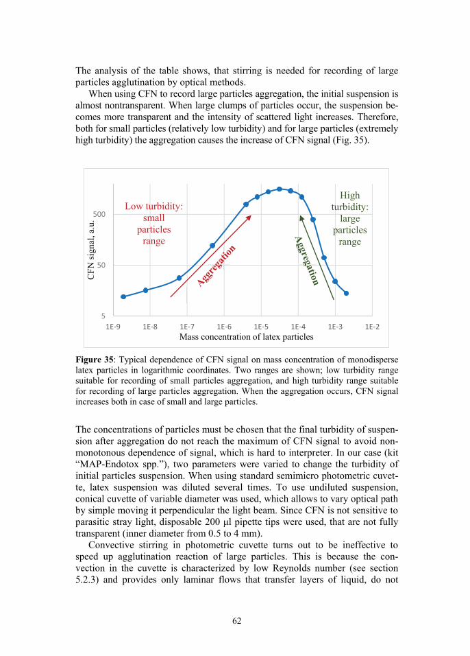
62

The analysis of the table shows, that stirring is needed for recording of large particles agglutination by optical methods.

When using CFN to record large particles aggregation, the initial suspension is almost nontransparent. When large clumps of particles occur, the suspension be-comes more transparent and the intensity of scattered light increases. Therefore, both for small particles (relatively low turbidity) and for large particles (extremely high turbidity) the aggregation causes the increase of CFN signal (Fig. 35).

Figure 35: Typical dependence of CFN signal on mass concentration of monodisperse latex particles in logarithmic coordinates. Two ranges are shown; low turbidity range suitable for recording of small particles aggregation, and high turbidity range suitable for recording of large particles aggregation. When the aggregation occurs, CFN signal increases both in case of small and large particles. The concentrations of particles must be chosen that the final turbidity of suspen-sion after aggregation do not reach the maximum of CFN signal to avoid non-monotonous dependence of signal, which is hard to interpreter. In our case (kit “MAP-Endotox spp.”), two parameters were varied to change the turbidity of initial particles suspension. When using standard semimicro photometric cuvet-te, latex suspension was diluted several times. To use undiluted suspension, conical cuvette of variable diameter was used, which allows to vary optical path by simple moving it perpendicular the light beam. Since CFN is not sensitive to parasitic stray light, disposable 200 μl pipette tips were used, that are not fully transparent (inner diameter from 0.5 to 4 mm).

Convective stirring in photometric cuvette turns out to be ineffective to speed up agglutination reaction of large particles. This is because the con-vection in the cuvette is characterized by low Reynolds number (see section 5.2.3) and provides only laminar flows that transfer layers of liquid, do not

5

50

500

1E-9 1E-8 1E-7 1E-6 1E-5 1E-4 1E-3 1E-2

CFN

sign

al, a

.u.

Mass concentration of latex particles

Low turbidity: small

particles range

High turbidity:

large particles

range

63

mixing them. Therefore, to increase the reaction rate, 3 turbulent methods of mixing were developed.

Method 1. The stirring in photometric cuvette can be created using so called “submerged jet”. Thin tube is inserted into the particles suspension and is con-nected hydrodynamically with a plunger pump. Plunger makes reciprocal motion; as a result, part of the liquid is periodically pulled in and pushed out from the tube (Fig. 36). To avoid contamination of the liquid, there can be membrane or simply air gap between the liquid and the plunger. When liquid is pushed out the tube, the submerged jet is produced providing turbulent flows in reaction mixture [ 28, p.118-121]. It increases reaction rate and redistribution of the formed aggregates in volume of the liquid.

Figure 36: A schematic of stirring by submerged jet, 1 – source of coherent light, 2 – cuvette, 3 – plunger pump, 4 – thin tube.

Method 2. The stirring in conical cuvette can be made using so called “diffuser flow”. Suspension of particles is moved along the conical cuvette, e.g. by plunger pump (Fig. 37). When liquid is flowing in the cuvette in the direction of its widening, turbulent flows are produced near cuvette walls already at low Reynolds numbers [ 28, p.113–118].

Figure 37: A schematic of stirring by diffuser flow, 1 – source of coherent light, 2 – conical cuvette, 3 – plunger pump.

1

2

4

3

1 2

3

64

Method 3. The stirring in any cuvette can be produced using magnetic particles, which are placed into the suspension of large functionalized particles. The surface of magnetic particles must be inert to the components of reaction mixture. The source of periodic magnetic field of low frequency, for example, rotating permanent magnet, causes the formation of rod-like structures and their cyclic movement in the liquid; such structures act as multitude of micro mag-netic stirrers, producing microturbulences [ 33] (Fig. 38). Besides, the concentra-tion and/or size of magnetic particles are chosen much less, than concentration and/or size of aggregating particles so that the intensity of light scattered by magnetic particles is much less than intensity of light scattered by reacting particles. Since the suspension of large particles is of high turbidity, the fulfill-ment of the requirement is quite real.

Figure 38: A schematic of stirring by diffuser flow, 1 – source of coherent light, 2 –cuvette, 3 – source of periodic magnetic field. Experiments were made using “CFN-2” prototype to record agglutination reactions with large particles (diagnostic kit “MAP-Endotox spp.”) in standard photometric semimicro cuvette and in conical cuvette (pipette tip).

Dependence curves of decimal logarithm of CFN signal on time are shown on Fig. 39 for different types of stirring in conical cuvette. All types of turbulent stirring increase the reaction rate manifold, especially combination of two turbulent stirrings.

Dependence curves of decimal logarithm of CFN signal on time is shown on Fig. 40 for different types of stirring in photometric cuvette. All types of turbu-lent stirring increase the reaction rate manifold.

3

1 2

65

Figure 39: Dependence curves of decimal logarithm of CFN signal (in a.u.) on time (in seconds) for different types of stirring in conical cuvette. The reaction of particles of diagnostic kit “MAP-Endotox spp.” with positive control is carried out; the control is added at time 0.

Figure 40: Dependence curves of decimal logarithm of CFN signal (in a.u.) on time (in seconds) for different types of stirring in photometric cuvette. The reaction of particles of diagnostic kit “MAP-Endotox spp.” with positive control is carried out; the control is added at time 0.

Convection Magnetic particlesDiffuser flow Diffuser flow + Magnetic particles

Convection Magnetic particles Submerged jet

66

To compare the effectiveness of intense but not turbulent stirring, the reaction was carried out in the cylindrical cuvette of 4 mm diameter with magnetic stirrer (platelet aggregation analyzer 220LA, Biola Ltd.) Standard magnetic stirring at 800 rpm was used, which produce circle laminar flows at Reynolds number of about 500, while the turbulent flows develop at Reynolds number of the order 104 [ 34]. The dependence curve of optical density on time is shown on Fig. 41, the reaction rate is much lower than when using turbulent stirring.

Figure 41: Dependence curve of optical density on time (in seconds) for 800 rpm magnetic stirring in cylindrical cuvette of 4 mm diameter. The reaction of particles of diagnostic kit “MAP-Endotox spp.” with positive control is carried out; the control is added at time 0.

5.5. Microbiological analyzer based on CFN By the results of investigation of CFN method, the area of laboratory diagnos-tics was chosen, where CFN would be efficient for solving the specific problem. The recommendations on the configuration of corresponding device design are given.

The chosen area of CFN applicability is clinical laboratory microbiology. In this field, high sensitivity is needed to detect low concentrations of microorga-nisms down to 103 CFU/ml [21], which cannot be provided by conventional nephelometry. Moreover, the automation of microbiological laboratories is of low level in comparison with other clinical laboratories [ 19], so the new devices are needed to increase the efficiency of analyses.

0

0,5

1

1,5

2

2,5

3

3,5

-100 400 900 1400 1900

Opt

ical

den

sity

Time, seconds

67

5.5.1. The recommendations on the development of microbiological CFN-analyzer

Microorganisms isolated from human biological liquids in microbiology labora-tories are bacteria and fungi. In most cases, they are bacteria, which can be rods and cocci (spherical). The most of pathogenic bacteria scatter light in average as spheres of 0.8 – 1.1 μm in diameter [ 9]. Since bacteria scatter light mostly in forward direction [ 10], to achieve maximum sensitivity, light scattered at low angles must be detected. CFN allows to use small scattering angles without complication of optical scheme and special requirement to cuvette quality, so CFN is suitable for construction of microbiological analyzer.

Bacterial growth is to be analyzed in broad range of concentration up to 109 CFU/ml. Since dynamic range of low-angle nephelometry is limited above (see Fig. 2, forward scattering), one has to use additional optical method to detect high bacterial concentration. The most suitable method is turbidimetry, which can be easily combined with CFN due to its low sensitivity to parasitic stray light.

Many small clinical microbiology laboratories receive 5-10 urine samples every day for testing. For that reason, microbiological CFN-analyzer has to be multichannel. Usually in multichannel laboratory analyzers one optical channel is used, which record the signal of multiple cuvettes one by one. For example, in microbiological analyzer HB&L carousel for 60 cuvettes with one optical channel is used. That is due to the complexity of optical system; using of mechanical system of cuvettes positioning is technologically simpler than using own source of light and detectors for each cuvette. Mechanical positioning system increases device complexity and cost and decreases its reliability. Technological simplicity of CFN and turbidimetry methods allow to use own laser diode and three silicon photodiodes (two for CFN and one for turbidimetry) for each cuvette, fully refusing mechanical moving parts in CFN-analyzer. On such principle, 12-channel CFN-analyzers “CFN-P-12” were built (Medtechnopark Ltd., Fig. 42).

68

Figure 42: Microbiological analyzer “CFN-P-12” (prototype).

The prototype is compact (30×20×15 cm3, <5 kg). Standard disposable photo-metric semimicro cuvettes are used, which are closed by disposable caps. Every cuvette is illuminated by its own laser diode with 650 nm wavelength. Light scattered at 7°-10° is detected.

The first prototype of microbiological analyzer “CFN-48” (Medtechnopark Ltd.) was constructed using mechanical positioning of the cuvettes for consecutive recording the signal from the cuvettes. 6 CFN channels were used, one for standard 8-well strip of 96-well plate, each well with 200 μl of liquid. Each strip was moved back-forward perpendicular to the laser beam. The prototype did not have turbidimetric detectors in addition to CFN. The experience of using this device confirmed the necessity of turbidimetry usage to increase the upper dynamic range limit. It also showed, that it is simpler to use its own optical system for each cuvette, than to construct precise cuvettes positioning system. Prototype also displayed that 200 μl cuvettes has too weak convection and it is preferable to use large cuvettes with 1 ml or more liquid in it. Prototype “CFN-48” is shown near two prototypes “CFN-P-12” on Fig. 43.

69

Figure 43: Prototypes of microbiological CFN-analyzers “CFN-48” и “CFN-P-12”.

According to the results of convective flows modeling (chapter 5.2.3), heater configuration №2 was used in prototype “CFN-P-12” to obtain more intensive stirring, than using heater №3, as in prototype “CFN-2”.

5.5.2. Microorganisms growth detection using CFN-analyzer

Combining CFN and turbidimetry allows to detect bacterial growth in broad range of concentrations from 103 CFU/ml to 109 CFU/ml. On Fig. 44, growth curves of clinical E. coli culture are shown, recorded by CFN and turbidimetry simultaneously using “CFN-P-12” prototype.

Figure 44: Growth curves of clinical E. coli culture recorded by CFN (blue) and turbidimetry (red) simultaneously using “CFN-P-12” prototype. Growth starts at about 103 CFU/ml and ends at about 109 CFU/ml.

70

In laboratory practice, detection limit of bacterial growth is usually restricted by turbidity of nutrient broth needed for bacteria to grow, which is usually not less than 103-104 CFU/ml. Turbidimetry allows to record very high turbidities: saturation of growth curve on Fig. 43 is caused not by limited sensitivity to high turbidities, but bacterial culture growth stationary phase [ 35]. So, constructed microbiological analyzer allows to record bacterial growth in all necessary range of concentrations.

5.5.3. Urine screening using CFN-analyzer

The first step to analyze urine sample received for bacteriological analysis is bacteriuria screening. Normally, urine is a sterile biological fluid, and the pre-sence of potentially pathogenic bacteria is called bacteriuria and indicates urinary tract infection. At the same time, skin and intestinal bacteria can be transferred to urine sample during urine collection. The main goal of bacteriuria screening is to determine the presence of microorganisms in urine, and to determine whether they are uropathogens or contamination. Urine samples are analyzed using microscope initially during general urine test. Such analysis is very simple but not enough sensitive for bacteria revealing [ 36], it also does not allow to distinguish uropathogens from contaminating flora and live microorga-nisms from lifeless. After general test, urine is seeded on solid nutrient media and left for 24-48 hours at 37°C. After incubation, every live bacterium forms the colony, so qualitative and quantitative composition of urine microflora can be assessed. Presence of high concentration of potential uropathogens is considered clinically significant with cut off level from 103 to 105 CFU/ml, depending on age, sex and clinical status of the patient [ 21].

When growth curves are recorded using optical methods, such as nephelo-metry and turbidimetry, urine sample is mixed with liquid nutrient broth, heated at 37°C and the changes in turbidity are analyzed. The advantage in comparison with culturing on solid media is that the time needed for growth detection reduces from at least 24 to 3–4 hours. The weak point of growth curve analysis is that the composition of urine is not analyzed. At the same time, samples with high concentration of contaminating flora can be distinguished from uropatho-gens, since contaminants need several hours to adapt to new medium [ 24]. So, growth is observed earlier in urine samples with true bacteriuria (uropathogens), than in samples with contamination (Fig. 45). The second parameter, that can be analyzed by CFN, but not by conventional nephelometry due to lack of sensiti-vity, is initial concentration of microorganisms. After fast centrifugation of urine for 1 minutes at ≈1700g (3000 rpm of standard laboratory centrifuge) all large impurities (such as human cells, salts and mucus) sediment on the bottom of the tube, and the microorganisms stay in the volume of the liquid. After such centrifugation, the turbidity of urine corresponds to the concentrations of the microorganisms in the urine, which is diagnostically useful parameter [ 25].

71

Figure 45: The examples of growth curves of microflora in three urine samples, recorded by “CFN-P-12” prototype. Two parameters are analyzed: the growth delay and the turbidity of urine samples.

Four studies were made to demonstrate the effectiveness of prototypes “CFN-P-12” for bacteriuria screening. The growth delay and turbidity of urine were ana-lyzed both separately and together. More than 650 urine samples were tested. The results of testing using CFN-analyzers were compared with the results obtained by classical method (culture on solid nutrient media), which was considered as gold standard. The highest sensitivity and specificity (95.2% and 96.9%) were achieved when analyzing both parameters together using CFN-analyzer (growth delay and turbidity of urine).

In one study urine samples were simultaneously analyzed using CFN proto-type and flow cytometry (UF-1000i). The comparison of the results showed significantly higher specificity of CFN (96.9%) in comparison with flow cyto-metry (82.3%) at the same sensitivity of both methods used (95.2%).

The results show that porotypes of microbiological analyzers “CFN-P-12” are effective for fast bacteriuria screening within 3-4 hours. 5.5.4. Rapid antibiotic susceptibility testing using CFN-analyzer

Microbiological analyzers based on optical methods allow to test antibiotic susceptibility of bacterial cultures. Growth curve of pure bacterial cultures are recorded in the presence of antibiotics in recommended concentration. The growth in the presence of the drug is compared with the control cuvette without antibiotic, growth inhibition is observed when the bacteria are sensitive (Fig. 46). In most cases, the antibiotics are taken in two concentrations [ 37, 38].

72

Figure 46: The example of susceptibility testing of clinical E. coli isolate to ceftriaxo-ne, recorded by “CFN-P-12” prototype.

Two studies were made to demonstrate the effectiveness of prototypes ‘CFN-P-12” for AST. More than 250 tests were made. The results were compared with widely used disk-diffusion method and serial dilution method, which take 20 hours. The agreement was from 84% to 88%. The obtained results showed that CFN is the promising method for fast antibiotic susceptibility testing within 3-6 hours.

73

6. MAIN ARGUMENTS PROPOSED

1. Physical processes underlying CFN were described and modeled, starting from light scattering by particles to the differential signal formation. The dependence of CFN signal on stirring was investigated; the stability of convection and its sufficiency for CFN functioning was demonstrated. Weak dependence of the signal on parasitic stray light was shown in comparison with conventional nephelometry allowing CFN to reach sensitivity as low as 103 CFU/ml.

2. CFN was applied to record immunoagglutination reactions in suspensions of small particles (size much less then wavelength) and large particles (size comparable of greater then wavelength). Three turbulent methods of mixing were developed to increase the reaction rate and standardize registration of agglutination of large particles.

3. The chosen area of CFN applicability is clinical laboratory microbiology due to high sensitivity is needed to detect low concentrations of micro-organisms down to 103 CFU/ml. Two main problems can be efficiently solved using CFN – urine screening and fast antibiotic susceptibility testing.

4. CFN method is suitable for registration of particles in broad range of concentrations and dispersion. The experience of CFN applying to bacterial growth recording allowed to determine the optimal parameters to develop CFN prototypes for clinical microbiology. The constructed prototypes “CFN-P-12” are 12-channeled, that allows to test 12 urine samples or susceptibility to 5 antibiotics at once. Light scattered at low angles (7°–10°) is detected to increase the detection limit of bacteria. The device is lack of mechanical system of cuvettes positioning; every cuvette is analyzed using its own laser and photodiodes, decreasing device complexity and increasing its reliability. In addition to CFN, turbidimetry is used to increase the upper limit of dynamic range to 109 CFU/ml.

5. Four studies was made to demonstrate the effectiveness of prototypes ‘CFN-P-12” for bacteriuria screening. More than 650 urine samples were analyzed. High sensitivity and specificity were shown (up to 95.2% and 96.9%) in comparison with classical methods (culture on solid nutrient media).

6. Two studies were made to demonstrate the effectiveness of prototypes ‘CFN-P-12” for antibiotic susceptibility testing. More than 250 tests were made; the agreement with classical methods (disk-diffusion and serial dilution methods) was from 84% to 88%.

74

SUMMARY IN ESTONIAN

Koherentse fluktuatsiooni nefelomeetria rakendamine laboratoorses praktikas

Doktoritöö põhieesmärk oli uurida ja optimeerida koherentse fluktuatsiooni nefelomeetria (CFN) meetodit, et arendada seadmeid, mis leiaks laialdast kasu-tust laboratoorses praktikas. Saavutati järgnevad põhitulemused. 1. Kirjeldati ning modelleeriti CFN meetodi aluseks olevaid füüsikalisi

protsesse. Uuriti CFN signaali sõltuvust lahuse mehaanilisest segamisest ja demonstreeriti konvektsioonivoolude stabiilsust küvetis ning piisavust CFN meetodi funktsioneerimiseks. Näidati signaali nõrka sõltuvust para-siitselt hajunud valguse hulgast võrrelduna tavalise nefelomeetria meeto-diga. See asjaolu võimaldab saavutada tundlikkust, et mõõta bakteri-kontsentratsioone kuni 103 CFU/ml .

2. Rakendati CFN meetodit, et monitoorida immunoglutinatsiooni reakt-sioone suspensioonides, mis koosnevad nii väikestest (osakeste suurused palju väiksemad kui lainepikkus) kui ka suurtest osakestest (osakeste suu-rused lainepikkusega võrreldavad või suuremad). Arendati kolm turbu-lentse segamise meetodit, et suurendada reaktsiooni kiirust ning standar-diseerida aglutinatsiooni registreerimist suurte osakeste puhul.

3. Sobiv rakendus CFN meetodile on kliiniline mikrobioloogia, kuna seal on vaja väga head tundlikkust, et avastada madala kontsentratsiooniga mikro-organisme kuni kontsentratsioonini 103 CFU/ml. Põhiprobleemid on või-malik efektiivselt lahendada CFN kasutades uriiniproovide kiir-skriiningut ja kiire antimikroobse tundlikkuse mõõtmine meetodit.

4. CFN meetod on sobiv osakeste registreerimiseks laias kontsentratsioonide vahemikus ning dispersioonides. Saadud kogemus CFN rakendamises bakteriaalse kasvu mõõtmiseks võimaldas kindlaks teha optimaalsed para-meetrid CFN seadme prototüübi koostamiseks kliinilise mikrobioloogia jaoks. Konstrueeritud prototüübid „CFN-P-12“ on 12-kanalilised, mis või-maldavad mõõta 12 uriiniproovi või 5 antibiootikumi mikroobtundlikkust ühekorraga. Et parandada tundlikkust bakterite minimaalse avastatava kontsentratsiooni väärtuste korral, detekteeritakse valgust, mis hajub väi-keste nurkade all (7°–10°). Seadmel puudub mehaaniline süsteem küvettide positsioneerimiseks; iga küvetti analüüsitakse tema enda laseri ja foto-dioodiga, vähendades nii seadme komplekssust ning suurendades töö-kindlust. Lisaks CFN-le kasutatakse seadmes turbidimeetriat, mis viib mõõteulatuse ülemise piiri 109 CFU/ml-ni.

5. Tehti neli kliinilist uuringut, et näidata „CFN-P-12“ prototüüpide efektiiv-sust bakteriuuria mõõtmisel. Analüüsiti rohkem kui 650 proovi. Näidati kõrget tundlikkust ning spetsiifilisust (vastavalt kuni 95.2% ja 96.9%) võrreldes klassikalise meetodiga (mikroobide külvamine tahkele toitekesk-konnale).

75

6. Tehti kaks kliinilist uuringut, et demonstreerida „CFN-P-12“ prototüüpide efektiivsust antibiootikumide mikroobitundlikkuse määramisel. Tehti roh-kem kui 250 mõõtmist; kooskõla klassikalise meetodiga (diskdifusiooni ning järjestikuse lahjendamise meetodid) oli 84% kuni 88%.

76

SUMMARY IN ENGLISH

Coherent fluctuating nephelometry application in laboratory practice

The main goal of the thesis was to investigate and optimize coherent fluctuation nephelometry (CFN) method to develop devices, oriented for wide use in laboratory practice. The fallowing results were obtained. 1. Physical processes underlying CFN were described and modeled. The

dependence of CFN signal on stirring was investigated; the stability of convection and its sufficiency for CFN functioning was demonstrated. Weak dependence of the signal on parasitic stray light was shown in com-parison with conventional nephelometry. That allows CFN to reach sensi-tivity as low as 103 CFU/ml.

2. CFN was applied to record immunoagglutination reactions in suspensions of small particles (size much less then wavelength) and large particles (size comparable of greater then wavelength). Three turbulent methods of mixing were developed to increase the reaction rate and standardize registration of agglutination of large particles.

3. The chosen area of CFN applicability is clinical laboratory microbiology due to high sensitivity is needed to detect low concentrations of micro-organisms down to 103 CFU/ml. Two main problems can be efficiently solved using CFN – urine screening and fast antibiotic susceptibility testing.

4. CFN method is suitable for registration of particles in broad range of con-centrations and dispersion. The experience of CFN applying to bacterial growth recording allowed to determine the optimal parameters to develop CFN prototypes for clinical microbiology. The constructed prototypes “CFN-P-12” are 12-channeled, that allows to test 12 urine samples or susceptibility to 5 antibiotics at once. Light scattered at low angles (7°–10°) is detected to increase the detection limit of bacteria. The device is lack of mechanical system of cuvettes positioning; every cuvette is analyzed using its own laser and photodiodes, decreasing device complexity and increasing its reliability. In addition to CFN, tubidimetry is used to increase the upper limit of dynamic range to 109 CFU/ml.

5. Four studies was made to demonstrate the effectiveness of prototypes ‘CFN-P-12” for bacteriuria screening. More than 650 urine samples were analyzed. High sensitivity and specificity were shown (up to 95.2% and 96.9%) in comparison with classical methods (culture on solid nutrient media).

6. Two studies were made to demonstrate the effectiveness of prototypes ‘CFN-P-12” for antibiotic susceptibility testing. More than 250 tests were made; the agreement with classical methods (disk-diffusion and serial dilution methods) was from 84% to 88%.

77

ACKNOWLEDGEMENTS

At first, I would like to thank my supervisors. I am very grateful to Dr. Alexey Volkov for teaching experimental methods and general support. Dr. Ilmo Sildos provided good assistance in studying and making the reports in Tartu Uni-versity.

Special thanks to Dr. Stanislav Rastopov for his outstanding engineering support.

I am grateful to Dr. Sergey Babichenko for help of various kinds; to Olga Shalatova for nutrient broths and antibiotics; to the coworkers from research-scientific laboratory in MONIKI, especially to Dr. Elena Rusanova for great support in the field of clinical microbiology.

Finally, I would like to thank my friends Mel and Will for loving and supporting me.

78

REFERENCES

1. Kober, P.A. and Graves, S.S., “Nephelometry (Photometric Analysis). I. History of Method and Development of Instruments”, Ind. Eng. Chem., 7(10), 843–847 (2014).

2. M.I.T. Quarterly, 13, 274 (1900). 3. McFarland, J., “The nephelometer: and instrument for estimating the number of

bacteria in suspensions used for calculation of opsonic index and for vaccines”, JAMA, 14, 1176–1178 (1907).

4. Kingsbury, F.B., Clark, C.P., Williams, G., and Post, A.L., “The rapid deter-mination of albumin in urine”, J. Lab. Clin. Med., 11, 981–989 (1926).

5. Sadar, M., “Turbidity Standards”, Hach Company Technical Information Series – Booklet No. 12, Hach Company, 1998.

6. Zapata, A. and Ramirez-Arcos, S., “A comparative study of McFarland turbidity standards and the Densimat photometer to determine bacterial cell density”, Curr Microbiol, 70(6), 907–909 (2015).

7. Maia, M.R., Marques, S., Cabrita, A.R., Wallace, R.J., Thompson, G., Fonseca, A.J., and Oliveira, H.M., “Simple and Versatile Turbidimetric Monitoring of Bacterial Growth in Liquid Cultures Using a Customized 3D Printed Culture Tube Holder and a Miniaturized Spectrophotometer: Application to Facultative and Strictly Anaerobic Bacteria”, Front Microbiol., 7, 1381 (2016).

8. Sadar, M., “Turbidity Science”, Hach Company Technical Information Series –Booklet No. 11, Hach Company, 1998.

9. Katz, A., Alimova, A., Xu, M., Rudolph, E., Shah, M.K., Savage, H.E., Rosen, R.B., McCormick, S.A., and Alfano, R.R., “Bacteria size determination by elastic light scattering”, IEEE J. Sel. Top. Quantum Electron., 9(2), 277–287 (2003).

10. Koch, A.L., “Theory of the angular dependence of light scattered by bacteria and similar-sized biological objects”, Theor. Biol., 18(1), 133–156 (1968).

11. U.S. EPA, “Detection of Biological Suspensions Using Online Detectors in a Drinking Water Distribution System Simulator”, U.S. Environmental Protection Agency, EPA/600/R-10/005 (2010).

12. Mindukshev, I., Gambaryan, S., Kehrer, L., Schuetz, C., Kobsar, A., Rukoyatkina, N., Nikolaev, V.O., Krivchenko, A., Watson, S.P., Walter, U., and Geiger, J., “Low angle light scattering analysis: a novel quantitative method for functional characterization of human and murine platelet receptors”, Clin. Chem. Lab. Med., 50(7), 1253–1262 (2012).

13. Galiano, P. and Mansutti, A., “Method for the bacteriological investigation of a biological sample and relative device”, Eur. Pat. Appl., EP2401355A1 (2010).

14. Cammings, H.Z. and Pike, E.R. (Eds.) “Photon Correlation Spectroscopy and Velocimetry”, Plenum. Press (1977).

15. Rastopov, S.F., “Coherent Fluctuation Nephelometry: a High-Sensitivity Method for Detecting Particles in Liquids”, Instrum. Exp. Tech., 54(6), 837–840 (2011).

16. Molina-Bolivar, J.A. and Galisteo-Gonzalez, F., “Latex immunoagglutination assays”, Polym. Rev., 45, 59–98 (2005).

17. Cox, A.J., DeWeerd, A.J., and Linden, J., “An experiment to measure Mie and Rayleigh total scattering cross sections”, Am. J. Phys., 70(6), 620–625 (2002).

18. Davenport, M., Mach, K.E., Dairiki Shortliffe, L.M., Banaei, N., Wang, T.H., and Liao, J.C., “New and developing diagnostic technologies for urinary tract infections”, Nat. Rev. Urol., 14(5), 296–310 (2017).

79

19. Bourbeau, P.P. and Ledeboer, N.A., “Automation in clinical microbiology”, J. Clin. Microbiol., 51(6), 1658–65 (2013).

20. Horcajada, J.P., Shaw, E., Padilla, B., Pintado, V., Calbo, E., Benito, N., Gamallo, R., Gozalo, M., and Rodríguez-Baño, J.; ITUBRAS group; GEIH; SEIMC, “Healthcare-associated, community-acquired and hospital-acquired bacteraemic urinary tract infections in hospitalized patients: a prospective multicentre cohort study in the era of antimicrobial resistance”, Clin. Microbiol. Infect., 19(10):962–968 (2013).

21. Kranz, J., Schmidt, S., Lebert, C., Schneidewind, L., Vahlensieck, W., Sester, U., Fünfstück, R., Helbig, S., Hofmann, W., Hummers, E., Kunze, M., Kniehl, E., Naber1, K., Mandraka, F., Mündner-Hensen, B., Schmiemann, G., and Wa-genlehner, F.M.E., “Epidemiology, diagnostics, therapy, prevention and mana-gement of uncomplicated bacterial outpatient acquired urinary tract infections in adult patients : Update 2017 of the interdisciplinary AWMF S3 guideline”, Urologe A., 56 (6), 746–758 (2017).

22. Hale, D.C., Wright, D.N., McKie, J.E., Isenberg, H.D., Jenkins, R.D., and Matsen, J.M., “Rapid screening for bacteriuria by light scatter photometry (Autobac): a collaborative study”, J. Clin. Microbiol., 13, 147–150 (1981).

23. Fontana, C.S., Favaro, M.A., Bossa, M., Minelli, S., Altieri, A., Pelliccioni, M., Falcione, F.T., Di Traglia, L., Cicchetti, O., and Favalli, C., “Improved diagnosis of central venous catheter-related bloodstream infections using the HB&L UROQUATTRO™ system”, Eur. J. Clin. Microbiol. Infect. Dis., 31(11), 3139–3144 (2012).

24. Lahanas, S., Stathopoulos, G., Chan, R.C., and van Hal, S.J., “Evaluation of the Alfred 60/AST device as a screening test for urinary tract infections”, J. Clin. Microbiol., 51(10), 3406–3408 (2013).

25. Herráez, O., Asencio, M.A., Carranza, R., Jarabo, M.M., Huertas, M., Redondo, O., Arias-Arias, A., Jiménez-Álvarez, S., Solís, S., Zamarrón, P., Illescas, M.S., and Galán, M.A., “Sysmex UF-1000i flow cytometer to screen urinary tract infections: the URISCAM multicentre study”, Lett. Appl. Microbiol., 66(3), 175-181 (2018).

26. http://webbook.nist.gov/chemistry/fluid/ 27. Ван де Хюлст, Г., “Рассеяние света малыми частицами”, Москва: Изда-

тельство иностранной литературы, 1961. (in Russian) 28. Ландау, Л.Д., Лифшиц, Е.М., “Теоретическая физика, т. 6, Гидродинамика”,

М.: Наука. Гл. ред. физ.-мат. лит., 1986. (in Russian) 29. Takai, N., Iwai, T., and Asakura, T., “Correlation distance of dynamic speckles”,

Appl. Opt., 22(1), 170-177 (1983). 30. Starovoytova T.A., Steriopolo, N.A., Zayko, V.V., and Vengerov, Yu.Yu., “The

latex agglutination with video digital registration: the enhancement of diagnostic significance of conventional technique”, Klin. Lab. Diagn., 2, 7-13 (2012). (in Russian)

31. Plotz, C.M. and Singer J.M., “The latex fixation test. I. Application to the serologic diagnosis of rheumatoid arthritis”, Am. J. Med., 21(6), 888-892 (1956).

32. Bangs Laboratories, “TechNote 304: Light-Scattering Assays”, Fishers: Bangs laboratories, 2008.

33. Lee, S.H., van Noort, D., Lee, J.Y., Zhang, B.T., and Park, T.H. “Effective mixing in a microfluidic chip using magnetic particles”, Lab on a Chip, 9(3), 479-482 (2009).

80

34. Forney, L.J., “Similitude in Stirred-Tank Reactors: Laminar Feed”, AIChE Jour-nal, 49 (10), 2655-2661, (2003).

35. Zwietering, M.H., Jongenburger, I., Rombouts, F.M., and van 't Riet, K., “Mo-deling of the bacterial growth curve”, Appl. Environ. Microbiol., 56(6), 1875-1881 (1990).

36. Cui, M., Ju, S., Shi, Y., and Jing, R, “Performance Verification of the Iris iQ200 Sprint Automated Urine Microscopy Analyzer in a Hospital Routine Laboratory”, Clin. Lab., 63(10), 1607-1612 (2017).

37. “Определение чувствительности микроорганизмов антибактериальным препаратам: Методические указания”, МУК 4.2.1890—04.—М.: Федераль-ный центр госсанэпиднадзора Минздрава России, 2004. (in Russian)

38. Коллектив авторов, “Определение чувствительности микроорганизмов к ан-тимикробным препаратам. Клинические рекомендации”, МАКМАХ (2015). (in Russian)

PUBLICATIONS

141

CURRICULUM VITAE

Name: Aleksandr Gurev Date of birth: 26 January 1987, Khimki, Moscow region, Russia Nationality: Russian Present Position: Senior researcher, M.F. Vladimirsky Moscow Regional

Clinical and Research Institute (MONIKI), Moscow, Russia Researcher, Medtechnopark Ltd., Moscow, Russia Address: Cherniyahovskogo 6–148, Moscow, Russia, 125319, Phone: +79060620673 E-mail: [email protected] Education: Federal Research and Clinical Center of Physical-Chemical Medicine,

Moscow, Russia (FRCC PCM), 2010–2014 post-graduate course Moscow Institute of Physics and Technology (MIPT), MSc 2010

(applied physics and mathematics) MIPT, BSc 2008 (applied physics and mathematics)

Language Skills: Russian (mother tongue) English (speaking, writing) Positions held: researcher, Medtechnopark Ltd. 2012– junior resercher, FRCC PCM 2014–2017 researcher, MONIKI 2017 senior researcher, MONIKI 2018– R&D Activity 1. Main research subjects: Coherent fluctuation nephelometry method

investigation with application in clinical laboratory practice 2. Publications included in the thesis:

1) Gur’ev, A.S.; Yudina, I.E.; Lazareva, A.V.; Volkov, A.Yu. Coherent fluctuation nephelometry as a promising method for diagnosis of bacteriuria. Practical Laboratory Medicine, in Press.

2) Gur’ev, A.S.; Kuznetsova, O.Yu.; Kraeva, L.A.; Rastopov, S.F.; Verbov, V.N.; Vasilenko, I.A.; Rusanova, E.V.; Volkov, A.Yu. (2018). Develop-ment of Microbiological Analyzer Based on Coherent Fluctuation Nephelometry. In: Hu Z., Petoukhov S., He M. (eds) Advances in Artifi-cial Systems for Medicine and Education, AIMEE 2017, Advances in Intelligent Systems and Computing, Springer, Cham, 658, 198–206; doi:10.1007/978-3-319-67349-3_18.

3) Gur’ev, A.S., Kuznetsova, O.Yu.; Pyasetskaya, M.F.; Smirnova, I.A.; Belyaeva, N.A.; Verbov, V.N.; Volkov, A.Yu. (2016). Raid urine screening for bacteriuria in children using microbiology analyzer,

142

combining photometric and coherent fluctuation nephelometric methods. Russian Journal of Infection and Immunity = Infektsiya i immunitet, 6(4), 395–398. Article in Russian; doi:10.15789/2220-7619-2016-4-395-398.

4) Gur’ev, A.S.; Volkov, A.Y.; Dolgushin, I.I.; Pospelova, A.V.; Rastopov, S.F.; Savochkina, A.Y.; Sergienko, V.I. (2015). Coherent Fluctuation Nephelometry: A Rapid Method for Urine Screening for Bacterial Conta-mination. Bulletin of experimental biology and medicine, 159(1), 107–110; doi:10.1007/s10517-015-2902-0.

5) Volkov, A.Y.; Gur’ev, A.S.; Levin, A.D.; Nijazmatov, A.A.; Rastopov, S.F. (2014). Optical method of registration of kinetics of particle aggre-gation in turbid suspensions. Patent of Russian Federation, RU2516193.

143

ELULOOKIRJELDUS

Nimi: Aleksandr Gurjev Sünniaeg: 26. jaanuar 1987, Himki, Moskva regioon, Venemaa Rahvus: venelane Praegune amet: vanem teaduslik töötaja, M.F. Vladimiri nimeline Moskva

Regionaalne Kliiniline ja Uurimisinstituut (MONIKI), Moskva, Venemaa

teadlane, Medtechnopark Ltd., Moskva, Venemaa Aadress: Tšernjahovski 6–148, Moskva, Venemaa, 125319, Telefon: +79060620673 E-post: [email protected] Haridus: Föderaalne Füüsikalis-Keemilise Meditsiini Uurimis- ja Kliiniline Keskus,

Moskva, Venemaa (FRCC PCM), 2010–2014 kraadiõppe kursus Moskva Füüsika ja Tehnoloogia Instituut (MIPT), MSc 2010

(rakendusfüüsika ja -matemaatika) MIPT, BSc 2008 (rakendusfüüsika ja -matemaatika)

Keeleoskus: vene (emakeel)

inglise (kõnes ja kirjas) Ametikohad: teadlane, Medtechnopark Ltd. 2012–

nooremteadlane, FRCC PCM 2014–2017 teadlane, MONIKI 2017 vanemteadlane, MONIKI 2018–

R&D tegevus 1. Peamised uurimisteemad: “Koherentse fluktuatsiooni nefelomeetria rakenda-

mine laboratoorses praktikas”. 2. Publikatsioonid, k.a. teesid:

1) Gur’ev, A.S.; Yudina, I.E.; Lazareva, A.V.; Volkov, A.Yu. Coherent fluctuation nephelometry as a promising method for diagnosis of bacteriuria. Practical Laboratory Medicine, in Press.

2) Gur’ev, A.S.; Kuznetsova, O.Yu.; Kraeva, L.A.; Rastopov, S.F.; Verbov, V.N.; Vasilenko, I.A.; Rusanova, E.V.; Volkov, A.Yu. (2018). Develop-ment of Microbiological Analyzer Based on Coherent Fluctuation Nephe-lometry. In: Hu Z., Petoukhov S., He M. (eds) Advances in Artificial Systems for Medicine and Education, AIMEE 2017, Advances in Intelli-gent Systems and Computing, Springer, Cham, 658, 198–206; doi:10. 1007/978-3-319-67349-3_18.

3) Gur’ev, A.S., Kuznetsova, O.Yu.; Pyasetskaya, M.F.; Smirnova, I.A.; Be-lyaeva, N.A.; Verbov, V.N.; Volkov, A.Yu. (2016). Raid urine screening

144

for bacteriuria in children using microbiology analyzer, combining photo-metric and coherent fluctuation nephelometric methods. Russian Journal of Infection and Immunity = Infektsiya i immunitet, 6(4), 395–398. Article in Russian; doi:10.15789/2220-7619-2016-4-395-398.

4) Gur’ev, A.S.; Volkov, A.Y.; Dolgushin, I.I.; Pospelova, A.V.; Rastopov, S.F.; Savochkina, A.Y.; Sergienko, V.I. (2015). Coherent Fluctuation Nephelometry: A Rapid Method for Urine Screening for Bacterial Conta-mination. Bulletin of experimental biology and medicine, 159(1), 107–110; doi:10.1007/s10517-015-2902-0.

5) Volkov, A.Y.; Gur’ev, A.S.; Levin, A.D.; Nijazmatov, A.A.; Rastopov, S.F. (2014). Optical method of registration of kinetics of particle aggre-gation in turbid suspensions. Patent of Russian Federation, RU2516193.

145


1. Andrus Ausmees. XUV-induced electron emission and electron-phonon interaction in alkali halides. Tartu, 1991.

2. Heiki Sõnajalg. Shaping and recalling of light pulses by optical elements based on spectral hole burning. Tartu, 1991.

3. Sergei Savihhin. Ultrafast dynamics of F-centers and bound excitons from picosecond spectroscopy data. Tartu, 1991.

4. Ergo Nõmmiste. Leelishalogeniidide röntgenelektronemissioon kiirita-misel footonitega energiaga 70–140 eV. Tartu, 1991.

5. Margus Rätsep. Spectral gratings and their relaxation in some low-temperature impurity-doped glasses and crystals. Tartu, 1991.

6. Tõnu Pullerits. Primary energy transfer in photosynthesis. Model calcula-tions. Tartu, 1991.

7. Olev Saks. Attoampri diapasoonis voolude mõõtmise füüsikalised alused. Tartu, 1991.

8. Andres Virro. AlGaAsSb/GaSb heterostructure injection lasers. Tartu, 1991. 9. Hans Korge. Investigation of negative point discharge in pure nitrogen at

atmospheric pressure. Tartu, 1992. 10. Jüri Maksimov. Nonlinear generation of laser VUV radiation for high-

resolution spectroscopy. Tartu, 1992. 11. Mark Aizengendler. Photostimulated transformation of aggregate defects

and spectral hole burning in a neutron-irradiated sapphire. Tartu, 1992. 12. Hele Siimon. Atomic layer molecular beam epitaxy of A2B6 compounds

described on the basis of kinetic equations model. Tartu, 1992. 13. Tõnu Reinot. The kinetics of polariton luminescence, energy transfer and

relaxation in anthracene. Tartu, 1992. 14. Toomas Rõõm. Paramagnetic H2– and F+ centers in CaO crystals: spectra,

relaxation and recombination luminescence. Tallinn, 1993. 15. Erko Jalviste. Laser spectroscopy of some jet-cooled organic molecules.

Tartu, 1993. 16. Alvo Aabloo. Studies of crystalline celluloses using potential energy calcu-

lations. Tartu, 1994. 17. Peeter Paris. Initiation of corona pulses. Tartu, 1994. 18. Павел Рубин. Локальные дефектные состояния в CuO2 плоскостях

высокотемпературных сверхпроводников. Тарту, 1994. 19. Olavi Ollikainen. Applications of persistent spectral hole burning in ultra-

fast optical neural networks, time-resolved spectroscopy and holographic interferometry. Tartu, 1996.

20. Ülo Mets. Methodological aspects of fluorescence correlation spectros-copy. Tartu, 1996.

21. Mikhail Danilkin. Interaction of intrinsic and impurity defects in CaS:Eu luminophors. Tartu, 1997.

146

22. Ирина Кудрявцева. Создание и стабилизация дефектов в кристаллах KBr, KCl, RbCl при облучении ВУФ-радиацией. Тарту, 1997.

23. Andres Osvet. Photochromic properties of radiation-induced defects in diamond. Tartu, 1998.

24. Jüri Örd. Classical and quantum aspects of geodesic multiplication. Tartu, 1998.

25. Priit Sarv. High resolution solid-state NMR studies of zeolites. Tartu, 1998. 26. Сергей Долгов. Электронные возбуждения и дефектообразование в

некоторых оксидах металлов. Тарту, 1998. 27. Kaupo Kukli. Atomic layer deposition of artificially structured dielectric

materials. Tartu, 1999. 28. Ivo Heinmaa. Nuclear resonance studies of local structure in RBa2Cu3O6+x

compounds. Tartu, 1999. 29. Aleksander Shelkan. Hole states in CuO2 planes of high temperature

superconducting materials. Tartu, 1999. 30. Dmitri Nevedrov. Nonlinear effects in quantum lattices. Tartu, 1999. 31. Rein Ruus. Collapse of 3d (4f) orbitals in 2p (3d) excited configurations

and its effect on the x-ray and electron spectra. Tartu, 1999. 32. Valter Zazubovich. Local relaxation in incommensurate and glassy solids

studied by Spectral Hole Burning. Tartu, 1999. 33. Indrek Reimand. Picosecond dynamics of optical excitations in GaAs and

other excitonic systems. Tartu, 2000. 34. Vladimir Babin. Spectroscopy of exciton states in some halide macro- and

nanocrystals. Tartu, 2001. 35. Toomas Plank. Positive corona at combined DC and AC voltage. Tartu, 2001. 36. Kristjan Leiger. Pressure-induced effects in inhomogeneous spectra of

doped solids. Tartu, 2002. 37. Helle Kaasik. Nonperturbative theory of multiphonon vibrational relaxa-

tion and nonradiative transitions. Tartu, 2002. 38. Tõnu Laas. Propagation of waves in curved spacetimes. Tartu, 2002. 39. Rünno Lõhmus. Application of novel hybrid methods in SPM studies of

nanostructural materials. Tartu, 2002. 40. Kaido Reivelt. Optical implementation of propagation-invariant pulsed

free-space wave fields. Tartu, 2003. 41. Heiki Kasemägi. The effect of nanoparticle additives on lithium-ion mobi-

lity in a polymer electrolyte. Tartu, 2003. 42. Villu Repän. Low current mode of negative corona. Tartu, 2004. 43. Алексей Котлов. Оксианионные диэлектрические кристаллы: зонная

структура и электронные возбуждения. Tartu, 2004. 44. Jaak Talts. Continuous non-invasive blood pressure measurement: compa-

rative and methodological studies of the differential servo-oscillometric method. Tartu, 2004.

45. Margus Saal. Studies of pre-big bang and braneworld cosmology. Tartu, 2004.

147

46. Eduard Gerškevitš. Dose to bone marrow and leukaemia risk in external beam radiotherapy of prostate cancer. Tartu, 2005.

47. Sergey Shchemelyov. Sum-frequency generation and multiphoton ioniza-tion in xenon under excitation by conical laser beams. Tartu, 2006.

48. Valter Kiisk. Optical investigation of metal-oxide thin films. Tartu, 2006. 49. Jaan Aarik. Atomic layer deposition of titanium, zirconium and hafnium

dioxides: growth mechanisms and properties of thin films. Tartu, 2007. 50. Astrid Rekker. Colored-noise-controlled anomalous transport and phase

transitions in complex systems. Tartu, 2007. 51. Andres Punning. Electromechanical characterization of ionic polymer-

metal composite sensing actuators. Tartu, 2007. 52. Indrek Jõgi. Conduction mechanisms in thin atomic layer deposited films

containing TiO2. Tartu, 2007. 53. Aleksei Krasnikov. Luminescence and defects creation processes in lead

tungstate crystals. Tartu, 2007. 54. Küllike Rägo. Superconducting properties of MgB2 in a scenario with

intra- and interband pairing channels. Tartu, 2008. 55. Els Heinsalu. Normal and anomalously slow diffusion under external

fields. Tartu, 2008. 56. Kuno Kooser. Soft x-ray induced radiative and nonradiative core-hole

decay processes in thin films and solids. Tartu, 2008. 57. Vadim Boltrushko. Theory of vibronic transitions with strong nonlinear

vibronic interaction in solids. Tartu, 2008. 58. Andi Hektor. Neutrino Physics beyond the Standard Model. Tartu, 2008. 59. Raavo Josepson. Photoinduced field-assisted electron emission into gases.

Tartu, 2008. 60. Martti Pärs. Study of spontaneous and photoinduced processes in mole-

cular solids using high-resolution optical spectroscopy. Tartu, 2008. 61. Kristjan Kannike. Implications of neutrino masses. Tartu, 2008. 62. Vigen Issahhanjan. Hole and interstitial centres in radiation-resistant MgO

single crystals. Tartu, 2008. 63. Veera Krasnenko. Computational modeling of fluorescent proteins. Tartu,

2008. 64. Mait Müntel. Detection of doubly charged higgs boson in the CMS detec-

tor. Tartu, 2008. 65. Kalle Kepler. Optimisation of patient doses and image quality in diag-

nostic radiology. Tartu, 2009. 66. Jüri Raud. Study of negative glow and positive column regions of capil-

lary HF discharge. Tartu, 2009. 67. Sven Lange. Spectroscopic and phase-stabilisation properties of pure and

rare-earth ions activated ZrO2 and HfO2. Tartu, 2010. 68. Aarne Kasikov. Optical characterization of inhomogeneous thin films.

Tartu, 2010. 69. Heli Valtna-Lukner. Superluminally propagating localized optical pulses.

Tartu, 2010.

148

70. Artjom Vargunin. Stochastic and deterministic features of ordering in the systems with a phase transition. Tartu, 2010.

71. Hannes Liivat. Probing new physics in e+e− annihilations into heavy particles via spin orientation effects. Tartu, 2010.

72. Tanel Mullari. On the second order relativistic deviation equation and its applications. Tartu, 2010.

73. Aleksandr Lissovski. Pulsed high-pressure discharge in argon: spectro-scopic diagnostics, modeling and development. Tartu, 2010.

74. Aile Tamm. Atomic layer deposition of high-permittivity insulators from cyclopentadienyl-based precursors. Tartu, 2010.

75. Janek Uin. Electrical separation for generating standard aerosols in a wide particle size range. Tartu, 2011.

76. Svetlana Ganina. Hajusandmetega ülesanded kui üks võimalus füüsika-õppe efektiivsuse tõstmiseks. Tartu, 2011

77. Joel Kuusk. Measurement of top-of-canopy spectral reflectance of forests for developing vegetation radiative transfer models. Tartu, 2011.

78. Raul Rammula. Atomic layer deposition of HfO2 – nucleation, growth and structure development of thin films. Tartu, 2011.

79. Сергей Наконечный. Исследование электронно-дырочных и интер-стициал-вакансионных процессов в монокристаллах MgO и LiF методами термоактивационной спектроскопии. Тарту, 2011.

80. Niina Voropajeva. Elementary excitations near the boundary of a strongly correlated crystal. Tartu, 2011.

81. Martin Timusk. Development and characterization of hybrid electro-optical materials. Tartu, 2012, 106 p.

82. Merle Lust. Assessment of dose components to Estonian population. Tartu, 2012, 84 p.

83. Karl Kruusamäe. Deformation-dependent electrode impedance of ionic electromechanically active polymers. Tartu, 2012, 128 p.

84. Liis Rebane. Measurement of the W cross section and a search for a doubly charged Higgs boson decaying to -leptons with the CMS detector. Tartu, 2012, 156 p.

85. Jevgeni Šablonin. Processes of structural defect creation in pure and doped MgO and NaCl single crystals under condition of low or super high density of electronic excitations. Tartu, 2013, 145 p.

86. Riho Vendt. Combined method for establishment and dissemination of the international temperature scale. Tartu, 2013, 108 p.

87. Peeter Piksarv. Spatiotemporal characterization of diffractive and non-diffractive light pulses. Tartu, 2013, 156 p.

88. Anna Šugai. Creation of structural defects under superhigh-dense irradiation of wide-gap metal oxides. Tartu, 2013, 108 p.

89. Ivar Kuusik. Soft X-ray spectroscopy of insulators. Tartu, 2013, 113 p. 90. Viktor Vabson. Measurement uncertainty in Estonian Standard Laboratory

for Mass. Tartu, 2013, 134 p.

149

91. Kaupo Voormansik. X-band synthetic aperture radar applications for environmental monitoring. Tartu, 2014, 117 p.

92. Deivid Pugal. hp-FEM model of IPMC deformation. Tartu, 2014, 143 p. 93. Siim Pikker. Modification in the emission and spectral shape of photo-

stable fluorophores by nanometallic structures. Tartu, 2014, 98 p. 94. Mihkel Pajusalu. Localized Photosynthetic Excitons. Tartu, 2014, 183 p. 95. Taavi Vaikjärv. Consideration of non-adiabaticity of the Pseudo-Jahn-

Teller effect: contribution of phonons. Tartu, 2014, 129 p. 96. Martin Vilbaste. Uncertainty sources and analysis methods in realizing SI

units of air humidity in Estonia. Tartu, 2014, 111 p. 97. Mihkel Rähn. Experimental nanophotonics: single-photon sources- and

nanofiber-related studies. Tartu, 2015, 107 p. 98. Raul Laasner. Excited state dynamics under high excitation densities in

tungstates. Tartu, 2015, 125 p. 99. Andris Slavinskis. EST Cube-1 attitude determination. Tartu, 2015, 104 p. 100. Karlis Zalite. Radar Remote Sensing for Monitoring Forest Floods and

Agricultural Grasslands. Tartu, 2016, 124 p. 101. Kaarel Piip. Development of LIBS for in-situ study of ITER relevant

materials. Tartu, 2016, 93 p. 102. Kadri Isakar. 210Pb in Estonian air: long term study of activity con-

centrations and origin of radioactive lead. Tartu, 2016, 107 p. 103. Artur Tamm. High entropy alloys: study of structural properties and

irradiation response. Tartu, 2016, 115 p. 104. Rasmus Talviste. Atmospheric-pressure He plasma jet: effect of dielectric

tube diameter. Tartu, 2016, 107 p. 105. Andres Tiko. Measurement of single top quark properties with the CMS

detector. Tartu, 2016, 161 p. 106. Aire Olesk. Hemiboreal Forest Mapping with Interferometric Synthetic

Aperture Radar. Tartu, 2016, 121 p. 107. Fred Valk. Nitrogen emission spectrum as a measure of electric field

strength in low-temperature gas discharges. Tartu, 2016, 149 p. 108. Manoop Chenchiliyan. Nano-structural Constraints for the Picosecond

Excitation Energy Migration and Trapping in Photosynthetic Membranes of Bacteria. Tartu, 2016, 115p.

109. Lauri Kaldamäe. Fermion mass and spin polarisation effects in top quark pair production and the decay of the higgs boson. Tartu, 2017, 104 p.

110. Marek Oja. Investigation of nano-size α- and transition alumina by means of VUV and cathodoluminescence spectroscopy. Tartu, 2017, 89 p.

111. Viktoriia Levushkina. Energy transfer processes in the solid solutions of complex oxides. Tartu, 2017, 101 p.

112. Mikk Antsov. Tribomechanical properties of individual 1D nanostruc-tures: experimental measurements supported by finite element method simulations. Tartu, 2017, 101 p.

113. Hardi Veermäe. Dark matter with long range vector-mediated inter-actions. Tartu, 2017, 137 p.

150

114. Aris Auzans. Development of computational model for nuclear energy systems analysis: natural resources optimisation and radiological impact minimization. Tartu, 2018, 138 p.

Coherent fluctuating nephelometry application in ...

Documents

Transcript of Coherent fluctuating nephelometry application in ...