COHERENCE FOR INVERTIBLE OBJECTS AND MULTI …ddugger/invcoh.pdf · At an even deeper level than...
38
COHERENCE FOR INVERTIBLE OBJECTS AND MULTI-GRADED HOMOTOPY RINGS DANIEL DUGGER Abstract. We prove a coherence theorem for invertible objects in a sym- metric monoidal category. This is used to deduce associativity, skew- commutativity, and related results for multi-graded morphism rings, gener- alizing the well-known versions for stable homotopy groups. Contents 1. Introduction 1 2. Review of MacLane’s coherence 9 3. Kelly-Laplaza coherence 11 4. Invertible objects 16 5. Coherence for invertible objects 22 6. The main applications: Z n -graded rings of maps 25 7. More general grading schema 31 Appendix A. A short motivic application 37 References 38 1. Introduction In algebraic topology a classical object of study is the stable homotopy ring π * (S), which is Z-graded and graded-commutative. For any topological space (or spectrum) X the stable homotopy groups π * (X) give a bimodule over π * (S). The motivation for the present paper comes from wanting to generalize this basic setup to more sophisticated homotopy theories, where the homotopy rings and mod- ules have a more elaborate grading. Standard examples are the categories of G- equivariant spectra and the category of motivic spectra. In these settings it has long been realized that it can be advantageous to use a grading by an index having to do with the invertible objects, rather than a grading by integers (which corre- spond to integral suspensions/desuspensions of the unit object). This paper deals with some fundamental questions that arise in this general situation. As we explain below, for general grading schema one must take some care over whether the analog of π * (S) is indeed associative, and whether the analogs of π * (X) are indeed bimodules. Care is also needed in the treatment of graded- commutativity. At an even deeper level than these issues, the ring structure on π * (S) is not exactly canonical—different choices in the basic setup can result in different isomorphism classes of rings. We approach these issues by proving a general coherence theorem for invertible objects in a symmetric monoidal category; 1
Transcript of COHERENCE FOR INVERTIBLE OBJECTS AND MULTI …ddugger/invcoh.pdf · At an even deeper level than...

COHERENCE FOR INVERTIBLE OBJECTS ANDMULTI-GRADED HOMOTOPY RINGS
DANIEL DUGGER
Abstract. We prove a coherence theorem for invertible objects in a sym-metric monoidal category. This is used to deduce associativity, skew-commutativity, and related results for multi-graded morphism rings, gener-alizing the well-known versions for stable homotopy groups.
Contents
1. Introduction 12. Review of MacLane’s coherence 93. Kelly-Laplaza coherence 114. Invertible objects 165. Coherence for invertible objects 226. The main applications: Zn-graded rings of maps 257. More general grading schema 31Appendix A. A short motivic application 37References 38
1. Introduction
In algebraic topology a classical object of study is the stable homotopy ringπ∗(S), which is Z-graded and graded-commutative. For any topological space (orspectrum) X the stable homotopy groups π∗(X) give a bimodule over π∗(S). Themotivation for the present paper comes from wanting to generalize this basic setupto more sophisticated homotopy theories, where the homotopy rings and mod-ules have a more elaborate grading. Standard examples are the categories of G-equivariant spectra and the category of motivic spectra. In these settings it haslong been realized that it can be advantageous to use a grading by an index havingto do with the invertible objects, rather than a grading by integers (which corre-spond to integral suspensions/desuspensions of the unit object). This paper dealswith some fundamental questions that arise in this general situation.
As we explain below, for general grading schema one must take some care overwhether the analog of π∗(S) is indeed associative, and whether the analogs ofπ∗(X) are indeed bimodules. Care is also needed in the treatment of graded-commutativity. At an even deeper level than these issues, the ring structure onπ∗(S) is not exactly canonical—different choices in the basic setup can result indifferent isomorphism classes of rings. We approach these issues by proving ageneral coherence theorem for invertible objects in a symmetric monoidal category;
1

2 DANIEL DUGGER
this is the main result of the paper, and is spread across Theorems 1.6, 1.10, 1.13,and 1.14 below. After establishing the coherence result we deduce the basic factsabout Zn-graded homotopy rings as consequences.
1.1. Introduction to the problem. Let (C,⊗) be a symmetric monoidal cate-gory, and let S denote the unit. Given objects x1, . . . , xn in C, we write x1⊗· · ·⊗xnas an abbreviation for
x1 ⊗ (x2 ⊗ (x3 ⊗ · · · (xn−1 ⊗ xn))).We also use xk as an abbreviation for x ⊗ x ⊗ · · · ⊗ x (k factors). So note thatx2⊗y3⊗z is an abbreviation for (x⊗x)⊗((y⊗(y⊗y))⊗z), and that by conventionx0 = S. Finally, for each tuple a = (a1, . . . , an) ∈ Nn, write
xa = xa11 ⊗ · · · ⊗ xan
n .
An object X of C is called invertible if there is an object Y and an isomorphismα : S → Y ⊗X. We will say that (Y, α) is an inverse for X. In this situation thereturns out to be a unique map α : X ⊗ Y → S such that the two evident maps from(X⊗Y )⊗X to X are the same, and this α is an isomorphism (see Proposition 4.11below). If a ∈ Z define
Xa =
{Xa (as already defined) if a ≥ 0,Y −a if a < 0.
Note that given an invertible object X, the isomorphism type of Y is uniquelydetermined; but given a specific choice of Y , the map α is not uniquely determined—it can be varied by an arbitrary element of Aut(S).
Let X1, . . . , Xn be a collection of invertible objects in C, with inverses(Y1, α1), . . . , (Yn, αn). For a ∈ Zn define
Xa = Xa11 ⊗ · · · ⊗Xan
n .
Assume now that C is an additive category and that the tensor product is anadditive functor in each variable. Let π∗(S) be the Zn-graded abelian group givenby πa(S) = C(Xa, S). More generally, if W is a fixed object in C let π∗(W ) be theZn-graded abelian group given by πa(W ) = C(Xa,W ). One of the goals of thispaper is the following:
Proposition 1.2.(1) π∗(S) is a Zn-graded ring,(2) π∗(W ) is a Zn-graded bimodule over π∗(S), and(3) There exist elements τ1, . . . , τn ∈ π(0,...,0)(S) satisfying τ2
i = 1 such that for allf ∈ πa(S) and g ∈ πb(S), where a, b ∈ Zn, one has
fg = gf ·[τ
(a1b1)1 · · · τ (anbn)
n
].
In fact, τi is just the trace of the identity map on Xi (see Section 3 for thedefinition of trace).
Remark 1.3. The groups π∗(W ) depend on the choice of objects X1, . . . , Xn, andtherefore we should probably write πX∗ (W ). We will always regard the sequenceX as being understood, however. Unfortunately, the ring structure from (1) de-pends on even more than this: it depends on the choices of α1, . . . , αn. Given onlythe sequence X, the number of isomorphism types of different ring structures isparameterized by the set Aut(S)n. See Proposition 7.1 below.

COHERENCE FOR INVERTIBLE OBJECTS AND MULTI-GRADED HOMOTOPY RINGS 3
To see the difficulty in (1), assume that f : Xa → S and g : Xb → S are two maps.Of course we may tensor them together to form f ⊗ g : Xa ⊗ Xb → S ⊗ S ∼= S.However, this only yields an element in πa+b(S) after choosing an isomorphismXa ⊗ Xb ∼= Xa+b. The trouble is that there are many such isomorphisms, andwe cannot just choose one at random. To ensure that π∗(S) is associative theseisomorphisms must be compatible in the sense that some evident pentagons allcommute.
Both (1) and (2) follow from the fact that one can choose such isomorphisms ina compatible way. This is not a particularly hard result, but it does require somecare. The skew-commutativity in (3) is more difficult, and when exploring this onequickly realizes the desirability of a general coherence theory for invertible objects.This paper develops such a theory.
Let us say a little more about skew-commutativity. Given an invertible object Xand a self-map f : X → X, there is a well-defined invariant tr(f) ∈ End(S) calledthe trace (see Section 3). Define τX = tr(idX) and call this the basic commuterfor the object X. One can prove in this generality that τX ∈ Aut(S) and satisfiesτ2X = idS . In fact τ gives a homomorphism Pic(C) → 2 Aut(S), where Pic(C)
is the group of isomorphism classes of invertible objects and 2 Aut(S) denotesthe 2-torsion elements in Aut(S). This homomorphism is a basic invariant of thesymmetric monoidal category, and governs all commutativity issues. See Section 4for more information.
The motivating examples for C one may wish to keep in mind throughout thepaper are:
• The G-equivariant stable homotopy category, where G is a finite group(or even a compact Lie group). In this case let V1, . . . , Vn be a collectionof finite-dimensional, irreducible, real representations for G that representevery isomorphism type. Let Xi = SVi be the suspension spectra of theone-point compactifications.
• The motivic stable homotopy category over some chosen ground ring. HereX1 = S1,0 and X2 = S1,1 are the two basic motivic spheres.
Remark 1.4. The product on π∗(S) defined above might look different from thestandard composition product that is used for stable homotopy groups. An easyargument shows that the products are, in fact, the same—see Remark 2.2.
1.5. Coherence results. Fix an invertible object X with inverse (Y, α). Let wbe a tensor word in X and Y . As a specific example, let us look at the wordw = (X ⊗ (X ⊗ Y )) ⊗ (Y ⊗ X). Clearly w ∼= X, but there are different ways toconstruct such an isomorphism. We might use the chain
w ∼= (X ⊗ S)⊗ (Y ⊗X) ∼= (X ⊗ S)⊗ S ∼= X
where we used α in the first isomorphism and α in the second. Or we might usethe chain
w ∼= (X ⊗ S)⊗ (Y ⊗X) ∼= X ⊗ (Y ⊗X) ∼= (X ⊗ Y )⊗X ∼= S ⊗X ∼= X
where we have used α in both the first isomorphism and in the fourth. Are thesetwo composite isomorphisms the same? Are all composite isomorphisms the same?
The answer to the second question depends on how careful we are. If we allowourselves to use the twist isomorphism t : X⊗X
∼=−→ X⊗X then it is not necessarily

4 DANIEL DUGGER
true that all composite isomorphisms will be the same. However, if we agree not touse the twist then we obtain the following result:
Theorem 1.6 (Coherence without twists). Let w1 and w2 be two tensor words inthe formal variables x and y. Suppose given two “formal composites” f, g : w1 → w2,by which we mean composable sequences of the following kinds of maps:
(i) associativity isomorphisms;(ii) unital isomorphisms S ⊗W ∼= W ∼= W ⊗ S;(iii) α and α;(iv) Maps obtained from the above ones by tensoring with identity maps;(v) Inverses of any of the above maps.
Then the maps f(C) and g(C), obtained by substituting X and Y for x and y andtaking the actual composite in C, are equal.
Example 1.7. The awkwardness in the statement of the above proposition iscommonplace in coherence results, because one has to eliminate certain accidentalcompositions from occurring. For example, suppose the invertible objectX happensto be its own inverse: i.e., suppose Y = X. Then both α and (α)−1 are mapsS → X ⊗ X; however, the theorem does not claim that they are the same map.Indeed, on a formal level α is a map S → yx and (α)−1 is a map S → xy, and sothere is no choice of w2 for which we can apply the theorem to these two maps.
Example 1.8. To complement the above “non-example” of the proposition, hereis a true application. Consider the words w1 = (x⊗ y)⊗ x and w2 = x. There aretwo formal compositions w1 → w2 we can construct as follows:
(x⊗ y)⊗ (x⊗ y) α⊗α−→ S ⊗ S∼=−→ S
and
(xy)(xy) // x(y(xy)) // x((yx)y)1⊗α−1⊗1// x(Sy) // xy α // S.
Note that we omitted the tensor symbols in the second composite for typographicalreasons. The proposition guarantees that the corresponding composites give thesame map in any symmetric monoidal category, for any invertible object X andinverse (Y, α).
Remark 1.9 (Canonical isomorphisms). Let X be an invertible object in C withinverse (Y, α). By a “tensor word” w in X and Y we can mean either a formalexpression in the symbols “X” and “Y ” or the actual object that results when theexpression is evaluated in C. We will usually let the reader deduce the meaningfrom context, but occasionally we will write w(C) for the latter interpretation—theevaluation of the formal word w inside of C. Formal tensor words are best thoughtof as functors into C where the allowable inputs are pairs (X, (Y, α)).
Consider the following statement: given a tensor word w as above, there is aunique a ∈ Z for which w ∼= Xa. This is true for formal tensor words, but notnecessarily true for their evaluations in C. For example, if our particular object Xis its own inverse (Y = X) then we have X ∼= X1 ∼= X−1 and so the value of ais not unique. But it is not true that the formal word “X” is isomorphic to theformal word “X−1”.
Keeping this nuance of language in mind, we can apply Theorem 1.6 as follows.Given a formal word w in X and Y , there is a unique a ∈ Z for which w ∼= Xa

COHERENCE FOR INVERTIBLE OBJECTS AND MULTI-GRADED HOMOTOPY RINGS 5
(canonical isomorphism of functors) and moreover the isomorphism can be chosenfrom the class described in Theorem 1.6, in which case it is canonical . In thispaper such canonical isomorphisms will always be denoted φ. The provision ofthese canonical isomorphisms is one of the main uses of coherence.
We will need a coherence theorem that is more sophisticated than Theorem 1.6.To state this, imagine that one has formal words w1, w2, . . . , wn in x and y togetherwith a string of maps
w1f1−→ w2
f2−→ · · · −→ wn−1fn−1−→ wn.
We assume that each fi is one of the following:(i) an associativity isomorphism;(ii) one of the unital isomorphisms S ⊗W ∼= W ∼= W ⊗ S;(iii) A twist map tx,x : x ⊗ x → x ⊗ x, tx,y : x ⊗ y → y ⊗ x, ty,x : y ⊗ x → x ⊗ y,
ty,y : y ⊗ y → y ⊗ y;(iv) Either α or α;(v) A map obtained from the above ones by tensoring with identity maps;(vi) An inverse of any of the above maps.Let (w, f) denote the tuple of wi’s and fi’s. Define the parity of (w, f) to be thetotal number of times tx,x, ty,y, tx,y and ty,x appear—that is, the number of i’s forwhich one of these maps appears as a tensor factor in fi.
Theorem 1.10 (Coherence with twists). Let (w, f) and (w′, f ′) be two strings asabove, and let k be the length of the first and l the length of the second. Assumethat w1 = w′1 and wk = w′l. If (w, f) and (w′, f ′) have the same parity, thenthe composite of the fi’s is equal to the composite of the f ′j’s in any symmetricmonoidal category, when x and y are replaced with an invertible object X and aninverse (Y, α).
Example 1.11. Consider the composites
Sα−→ Y ⊗X tY,X−→ X ⊗ Y α−→ S
andS
φ−→ (Y ⊗ Y )⊗ (X ⊗X) id⊗tX−→ (Y ⊗ Y )⊗ (X ⊗X)φ−1
−→ S
where φ is the canonical isomorphism provided by Theorem 1.6. Then Theorem 1.10states that these two composites are the same. An attempt to prove this directlywill quickly demonstrate the nontriviality of Theorem 1.10.
Now we turn to coherence theorems involving several different invertible ob-jects. Suppose again that X1, . . . , Xn are invertible objects in C. For each i, let(X−1
i , αi) denote a chosen inverse for Xi. Let w be a tensor word in X1, . . . , Xn
and X−11 , . . . , X−1
n . It is clear that w is formally isomorphic to Xa for a uniquelydetermined a ∈ Zn. We want a result which says that different ways of constructingsuch an isomorphism yield the same result.
Remark 1.12. In our statements of the next two results we dispense with thephrasing about formal compositions and their instances inside of a given symmetricmonoidal category. However, this language should be taken as implicit in thestatements.

6 DANIEL DUGGER
Theorem 1.13 (Coherence without self-twists, multi-object case). Let w be atensor word in the symbols Xi and X−1
i , 1 ≤ i ≤ n. There is an isomorphismw ∼= Xa constructed as a composite of the following kinds of maps, and moreoverthis isomorphism is unique. The maps we are allowed to use are
(i) associativity isomorphisms;(ii) unital isomorphisms;(iii) commutativity isomorphisms Xi⊗Xj → Xj ⊗Xi and Xi⊗X−1
j → X−1j ⊗Xi
for i 6= j;(iv) the maps αi and αi;(v) maps obtained from (i)–(iv) by tensoring with identities;(vi) all inverses of maps in (i)–(v).
We also have a more general version involving parity checks. Supposew1, w2, . . . , wk are tensor words in the Xi’s and X−1
i ’s, and consider a compos-ite
w1f1−→ w2
f2−→ · · · −→ wk−1fk−1−→ wk.
We assume that each fi is one of the following:(i) an associativity isomorphism;(ii) one of the unital isomorphisms S ⊗W ∼= W ∼= W ⊗ S;(iii) A twist map tXi,Xj
: Xi ⊗Xj → Xj ⊗Xi, tXi,X−1j
: Xi ⊗X−1j → X−1
j ⊗Xi,
tX−1i ,Xj
: X−1i ⊗Xj → Xj ⊗X−1
i , or tX−1i ,X−1
j: X−1
i ⊗X−1j → X−1
j ⊗X−1i ,
where possibly i = j;(iv) One of the αi’s or αi’s;(v) A map obtained from the above ones by tensoring with identity maps;(vi) An inverse of any of the above maps.Define the i-parity of the string (w, f) to be the total number of times tXi,Xi ,tXi,X
−1i
, tX−1i ,Xi
, and tX−1i ,X−1
iappear in the fj ’s. We have the following:
Theorem 1.14 (Coherence with self-twists, multi-object case). Let (w, f) and(w′, f ′) be two strings as above, where the length of the first is k and the length ofthe second is l. Assume w1 = w′1 and wk = w′l. If (w, f) and (w′, f ′) have the samei-parity for all 1 ≤ i ≤ n, then the composites of the two strings are the same map.
1.15. Applications. The first application answers the question raised at the be-ginning of the paper. If f ∈ πa(S) and g ∈ πb(S) then form the tensor productf ⊗ g : Xa ⊗ Xb → S ⊗ S ∼= S. Theorem 1.13 supplies a canonical isomorphismXa ⊗Xb → Xa+b, and using this we obtain an element f · g ∈ πa+b(S). Similarly,one obtains maps πa(S)⊗ πb(W ) → πa+b(W ) and so forth. Coherence guaranteesthat these pairings all have the desired associativity (see Section 2 for details).
Given a map f : Xa → Xb there are two evident ways to recover an elementof πa−b(S). We can tensor on the left with X−b and then use the canonical iso-morphisms from Theorem 1.13, or we can tensor on the right and use canonicalisomorphisms. We call the associated elements [f ]r and [f ]l, respectively. Anotherapplication of coherence is to relate these two elements:
[f ]r = [f ]l ·∏
τbi(ai−bi)i(1.16)
where the τi’s are the basic commuters of the Xi’s. This and many related formulasare developed in Section 6.

COHERENCE FOR INVERTIBLE OBJECTS AND MULTI-GRADED HOMOTOPY RINGS 7
Let us very briefly indicate the idea behind skew-commutativity. If f : Xa → Sand g : Xb → S then we may form the diagram
Xa ⊗Xb
ta,b
��
f⊗g // S ⊗ S S.
Xb ⊗Xa
g⊗f
99ttttttttt
A little work gives that inside π∗(S) we have f ·g = g ·f · [ta,b]r (note that by (1.16)one has [ta,b]r = [ta,b]l). The content of Proposition 1.2(c) is the identification of[ta,b]r as a product of basic commuters; this is a direct consequence of Theorem 1.14,which says that the associated composite S → S is determined purely by the paritiesinvolved. See Section 6 for complete details.
1.17. The stable motivic homotopy ring. We close this long introduction witha very specific example. In the stable motivic homotopy category (over a chosenground field) there are two basic spheres denoted S1,0 and S1,1. These are invertibleobjects. More generally one sets Sp,q = (S1,0)∧(p−q) ∧ (S1,1)∧(q), for any p, q ∈ Z.The bigraded stable homotopy ring π∗,∗(S) is an instance of the general situationconsidered in this paper, although unfortunately the bigrading is different fromthe generic bigrading we adopted for Proposition 1.2: the motivic group πa,b(S)corresponds to what we have been calling π(a−b,b)(S).
The basic commuter for S1,0 is the element −1 ∈ π0,0(S). The basic commuterfor S1,1 is represented by the twist map S1,1 ∧ S1,1 → S1,1 ∧ S1,1; in motivichomotopy theory it is usually denoted ε ∈ π0,0(S). The skew-commutativity resultfor the motivic stable homotopy ring is the following, obtained as a direct corollaryof Proposition 1.2:
Proposition 1.18. For f ∈ πa,b(S) and g ∈ πc,d(S) one has
fg = gf · (−1)(a−b)(c−d) · εbd.
Now assume that the ground field is C, so that there is a realization map ψfrom the stable motivic homotopy category to the classical stable homotopy cat-egory of topological spaces. This induces a collection of group homomorphismsψp,q : πp,q(S)→ πp(S). One’s first guess might be that these maps assemble into aring homomorphism ψ : π∗,∗(S)→ π∗(S), but this is not quite right. Instead thereis the following identity:
Proposition 1.19. For f ∈ πa,b(S) and g ∈ πc,d(S) one has
ψ(fg) = ψ(f) · ψ(g) · (−1)b(c−d).
This result was one of the motivations for the work in this paper; we include theproof as a brief appendix.
Remark 1.20. It is satisfying to check that Propositions 1.18 and 1.19 are (takentogether) compatible with the graded-commutativity of the classical stable homo-topy ring. This uses that ψ(ε) = −1.

8 DANIEL DUGGER
1.21. Generalizations. Let Pic(C) be the group of isomorphism classes of invert-ible objects in C. Let A be an abelian group and let h : A→ Pic(C) be a homomor-phism (the case A = Pic(C) is the main one of interest, but it is useful to work inslightly greater generality). The question we pose is whether π(S) can be regardedas an A-graded ring. We can certainly choose, for each a ∈ A, an object Xa in theisomorphism class h(a). We can then define an A-graded abelian group by
πAa (S) = C(Xa, S).
To give a pairing on this graded group one should start by choosing isomorphismsσa,b : Xa+b → Xa ⊗ Xb, and for the pairing to be associative these isomorphismsmust satisfy a certain compatibility condition (a unital condition should also beimposed). Our coherence results show that when A is finitely-generated and freethis can be accomplished—although it is important to realize that the method fordoing so is not quite canonical, depending both on a choice of basis for A and achoice of the αi maps we encountered earlier. What about other values of A? Wewill show that(1) For any abelian group A, the isomorphisms σa,b can be chosen so that πA∗ (S)
is an associative and unital ring;(2) However, the choices involved in (1) are not canonical and the different isomor-
phism classes of rings one can obtain are in bijective correspondence with theelements of the group cohomology H2(A; Aut(S)).
In homotopy theory one often hears the slogan “one should grade things by theinvertible objects”; point (2) above suggests that this is a little more dicey thanone might wish. These results are in Section 7.
1.22. Some background, and an apology. From a certain perspective this pa-per is entirely on the subject of getting signs correct—although the “signs” are notjust ±1 but rather elements in the 2-torsion of Aut(S), where (C,⊗, S) is a sym-metric monoidal category. Many of the results are undoubtedly folklore, but justlacking a convenient reference. Since this is a subject where it seems particularlyimportant to have a convenient reference—no one likes to think about signs—wehave included quite a bit of exposition (perhaps overdoing it on occasion).
Associativity and commutativity for RO(G)-graded stable homotopy rings havetypically been dealt with in a somewhat different way than what we describe here.In essence, the various choices for isomorphisms are built into the framework fromthe very beginning, and one is tasked with keeping track of them. We refer thereader to [Ma, Chapter 13, Section 1] and [MS, Section 21.1] for detailed discussions.
Certainly Proposition 1.2 and related results are if not well-known then at leastnot surprising—although I wonder if the sign in the multiplicativity of the forgetfulmap (see Proposition 1.19) has been noticed before, either in the motivic or equi-variant context. I have also been unable to find a reference in the literature similarto Proposition 6.11, even though the sign questions dealt with by that result areubiquitous.
Invertible objects are well-studied in the literature (for example, in [FW]), butin somewhat sporadic places—and there seem to be some gaps. For a self-mapf : X → X where X is invertible, there are two ways to obtain an element ofEnd(S). One is called the trace of f , and the other is something that does not havea standard name—in this paper we call it the D-invariant . These two invariants

COHERENCE FOR INVERTIBLE OBJECTS AND MULTI-GRADED HOMOTOPY RINGS 9
can be different, although they sometimes get confused. We attempt to give acareful treatment in Section 4.
As far as the coherence statements are concerned, the earliest result along theselines seems to be [D, Lemma 1.4.3], due to Deligne. However, Deligne’s result(stated without proof) only applied to symmetric monoidal categories where theself-twists X⊗X → X⊗X are all equal to the identity; as is clear from the resultslisted above, this omits the important and nontrivial phenomena that occur in thegeneral case. Symmetric monoidal categories in which all objects are invertible aretreated again in [FW]. A classification theorem is given (see [FW, Corollary 6.6]),from which coherence results are easily deducible, but again only in the case wherethe self-twists are all equal to the identity. Another sort of classification theoremfor such categories is given in the unpublished PhD thesis [H, Chapter II, Section2, Proposition 5]; but although Hoang’s theorem allows for non-identity self-twiststhe classification is of a different nature and does not seem to yield any coherenceresults. The excellent and influential paper [JS] has coherence results in the braidedcontext, but not for invertible objects; it gives a classification theorem for braidedmonoidal categories where all objects are invertible, but again not yielding coher-ence results in any evident way. The literature contains many more sophisticatedcoherence results than the ones presented here, and so it seems to be merely anunfortunate accident that there is no convenient reference for them.
1.23. Organization of the paper. In Section 2 we give a brief review ofMacLane’s coherence theorem for monoidal categories, and explain how it gives riseto associativity results for N-graded morphism groups. Section 3 then reviews thedeeper coherence theorem of Kelly-Laplaza, which applies to symmetric monoidalcategories with left duals. Section 4 develops the basic theory of invertible objects,in particular establishing that the trace of the identity map on such an object hasorder at most two; this is a key result used throughout the paper. In Section 5 weprove the coherence theorems for invertible objects, and in Section 6 we give theapplications to Zn-graded morphism rings. Finally, Section 7 deals with the topicof grading morphism rings by non-free abelian groups.
1.24. Acknowledgements. This research was partially supported by NSF grantDMS-0905888. The author is grateful to Sharon Hollander, Peter May, VictorOstrik, and Vadim Vologodsky for helpful conversations.
2. Review of MacLane’s coherence
Here we recall how MacLane’s classical coherence theorem for symmetricmonoidal categories gives rise to an associativity result for Nn-graded morphismrings.
Let (C,⊗, S) be a symmetric monoidal category. Where needed, we will denotethe associativity isomorphism (x ⊗ y) ⊗ z ∼= x ⊗ (y ⊗ z) by a and the symmetryisomorphism x⊗ y ∼= y ⊗ x by t.
Let w be any tensor word made up of formal variables xi—for instance, the word((x1 ⊗ x2) ⊗ x1) ⊗ (x2 ⊗ x3) is one example. Such tensor words can be identifiedwith certain kinds of functors Cn → C, where n is the number of letters in theword. Precisely, these are the functors that can be built up from ⊗ : C2 → C usingcomposition and the operation of cartesian product with identity maps.

10 DANIEL DUGGER
Using the associativity and commutativity isomorphisms, there is a “formal iso-morphism” (or natural isomorphism) between w and some word xa, for a uniquelydetermined a ∈ Nn. To fix such an isomorphism, here is what we do. First, re-label the x1’s in w as x1a, x1b, x1c, etc., with the indices appearing alphabeticallyfrom left to right in the word. Do the same for all the other xi’s. Let w′ denotethe new word thus constructed. Regard w′ as a functor CN → C, where N isthe total number of variables in w′. Using the associativity, commutativity, andunital isomorphisms one can construct a natural isomorphism between the functorcorresponding to w′ and the functor corresponding to the word
(x1a ⊗ x1b ⊗ · · · )⊗ (x2a ⊗ x2b ⊗ · · · )⊗ · · · ⊗ (xna ⊗ xnb ⊗ · · · ).Moreover, MacLane’s coherence theorem [M, Theorem XI.1.1] says that this nat-ural isomorphism is uniquely determined . The exact choices of associativity andcommutativity isomorphisms used to construct it are definitely not unique, but thecomposite isomorphism itself is unique. Now evaluate this natural isomorphism inthe case where all the x1,∗ objects are equal to x1, all the x2,∗ objects are equal tox2, etc. This is our definition of φ : w
∼=−→ xa
Using the observation of the last paragraph, for a, b ∈ Nn we obtain canonicalisomorphims
φa,b : xa ⊗ xb∼=−→ xa+b
such that the following diagram commutes:
(xa ⊗ xb)⊗ xc∼= //
φa,b⊗id
��
xa ⊗ (xb ⊗ xc)
id⊗φb,c
��xa+b ⊗ xc
φa+b,c ''OOOOOOOOOO xa ⊗ xb+c
φa,b+cwwoooooooooo
xa+b+c.
(2.1)
The reason it commutes is again by the coherence theorem. Both ways of movingaround the diagram are instances of a natural transformation made up of the asso-ciativity and commutativity isomorphisms, where one relabels the x1’s appearingas x1a, x1b, etc., and the same for the other variables. MacLane’s theorem saysthat there is a unique such natural transformation, and so the two ways of movingaround the diagram must be the same. (Note also that when a or b is the zero vectorthen φa,b is the unital isomorphism from the symmetric monoidal structure).
Now assume that C is also an additive category, and that the tensor product isan additive functor in each variable. Let X1, . . . , Xn be fixed objects in C. Considerthe Nn-graded abelian group
R = ⊕a∈NnC(Xa, S).
We will also write Ra for C(Xa, S). We claim that R has the structure of an Nn-graded ring. The product is defined as follows. If f ∈ Ra and g ∈ Rb, definefg ∈ Ra+b to be the composition
Xa+bφ−1
a,b−→ Xa ⊗Xb f⊗g−→ S ⊗ S ∼= S.

COHERENCE FOR INVERTIBLE OBJECTS AND MULTI-GRADED HOMOTOPY RINGS 11
Remark 2.2. Note that the above product can also be described as the composition
Xa+b ∼= Xa ⊗Xb id⊗g−→ Xa ⊗ S f⊗id−→ S ⊗ S ∼= S.
In this way the product in R can be thought of as induced by the composition inthe category C: fg comes from composing f with an appropriately “suspended”version of g.
Proposition 2.3. R is a graded ring (associative and unital), and R0 is central.
Proof. Distributivity follows immediately from the fact that ⊗ is biadditive: forinstance, if f, g ∈ Ra and h ∈ Rb then the map (f+g)⊗h is equal to (f⊗h)+(g⊗h).So the same remains true when we precompose both with φ−1
a,b.Associativity follows, by an easy argument, from the fact that diagram (2.1) is
commutative. The fact that φa,b equals the unital isomorphism when a or b is zeroimplies that the identity element idS ∈ R0 is a unit for R.
For the centrality of R0, let f : S → S and let g : Xa → S. The following diagramis commutative:
Xa ⊗ S
t
��
g⊗f // S ⊗ S
t
��
∼=
%%LLLLLLL
Xa
∼= 77ppppppp
∼= ''NNNNNNN S
S ⊗Xa
f⊗g// S ⊗ S
∼=
99rrrrrrr
The composition across the top is f · g, and across the bottom is g · f . �
Remark 2.4. This section serves as the prototype for what will happen in therest of the paper. In the case where the objects Xi are invertible under the tensorproduct, we wish to extend R to a Zn-graded ring. This requires extending theconstruction of the φa,b’s, which in turn depends on a more sophisticated versionof coherence.
3. Kelly-Laplaza coherence
Let U be a set. Kelly and Laplaza [KL] describe the “free symmetric monoidalcategory with left duals” on the set U, denoted here KL(U). In this section wereview this construction.
3.1. Preliminaries. Let (C,⊗, S) be a symmetric monoidal category, and let Xbe an object. Recall that a left dual for X is an object Y together with mapsα : S → Y ⊗X and α : X ⊗ Y → S such that the composites
X = X ⊗ S id⊗α−→ X ⊗ Y ⊗X α⊗id−→ S ⊗X = X
andY = S ⊗ Y α⊗id−→ Y ⊗X ⊗ Y id⊗α−→ Y ⊗ S = Y
are the respective identities (we are not bothering to write the associativity isomor-phisms in the composites, even though they are there). To give an object Z thestructure of a left dual of X is the same as giving the functor Z⊗ (−) the structureof a right adjoint to X ⊗ (−). This observation makes it clear that if (Y, α, α) and(Y ′, α′, α′) are both left duals for X then there is a unique isomorphism Y → Y ′
that is compatible with the extra structure.
12 DANIEL DUGGER
Definition 3.2. A symmetric monoidal category with left duals is a sym-metric monoidal category (C,⊗, S) together with an assignment X 7→ (X∗, αX , αX)that equips every object of C with a left dual. (Warning: Note that (X∗)∗ need notequal X, although they will be isomorphic).
In the above setting, there is a unique way of making X → X∗ into a contravari-ant functor. This is not included as part of the definition only to minimize thenumber of things that need to be checked in applications. We will not need thefunctoriality of duals.
It is easy to see that any closed symmetric monoidal category has left duals.Suppose X has a left dual and f : X → X is a map. Then we may form the
compositeS
α−→ X∗ ⊗X id⊗f−→ X∗ ⊗X t−→ X ⊗X∗ α−→ S,
and this composite is called the trace of f . The uniqueness of left duals (up toisomorphism) shows that tr(f) is not dependent on the choice of left dual for X.
The trace satisfies the following properties:
Proposition 3.3. Let C be a symmetric monoidal category with left duals.(a) If there is a commutative diagram
Xq //
f
��
Z
g
��X
q // Z
in which q is an isomorphism, then tr(f) = tr(g).(b) If f : X → Y and g : Y → X then tr(fg) = tr(gf).
Proof. For part (a), observe that if (X∗, α, α) is a left dual for X then X∗ is also aleft dual for Z via the maps α′ = (idX∗ ⊗q)α and α′ = α(q−1 ⊗ idX∗). Using this,(a) is an easy exercise.
Part (b) is much harder. It is not needed in the present paper, but included forexpository purposes. For a proof, see [PS, Proposition 2.4]. �
We will also need the following fundamental result:
Lemma 3.4. In a symmetric monoidal category the monoid End(S) is abelian.
Proof. Suppose f, g : S → S and consider the following commutative diagram:
S ⊗ Sf⊗id //
��
S ⊗ Sid⊗g //
��
S ⊗ S
��S
f // Sg // S.
This shows that gf is the composite
S∼=−→ S ⊗ S f⊗g−→ S
∼=−→ S.
A similar diagram also shows that fg is also equal to this composite, so gf = fg. �

COHERENCE FOR INVERTIBLE OBJECTS AND MULTI-GRADED HOMOTOPY RINGS 13
3.5. The construction. For any category U the paper [KL] constructs the freesymmetric monoidal category with left duals on U. We will only need this con-struction where U only has identity maps—i.e., U is just a set. See Remark 3.7,however, for hints about the general case.
Note that for every element X ∈ U our category must have an identity map idXand therefore a self-map of S obtained by taking the trace. These traces will allneed to commute, since all self-maps of S commute by Lemma 3.4. So let N〈U〉be the free commutative monoid on the set U. If X ∈ U we think of the element[X] ∈ N〈U〉 as the formal trace of the identity map on X. Our construction forKL(U) will have N〈U〉 as its set of self-maps of S.
Define a signed set to be a set A together with a function τ : A → {+,−}. IfA is a signed set let A∗ be the same set but with the signs reversed. If A and Bare signed sets then A q B denotes the disjoint union with the evident signs. Abipartition of a signed set A is a directed graph with A as the vertex set, havingthe properties that
(i) The tail of every edge is marked with − and the head of every edge is markedwith +;
(ii) Every element of A is a vertex of exactly one edge.If A and B are signed sets, then a correspondence from A to B is a bipartitionof A∗ q B. One can make a picture of such a thing by drawing the elements of Aon one “level”, the elements of B on a lower level, and then drawing the edges ofthe bipartition. For example:
A : +
��@@@
@@@@
+
��~~~~
~~~
+ ??− −
B : + + −
77oooooooooooooo −��+
Note the convention for drawing edges with vertices at the same level: if the verticesare on the top level we draw a cup ∪, and if the vertices are on the bottom levelwe draw a cap ∩. Also, there is a simple technique for getting the direction of thearrows straight: each element with sign + should be pictured as a small downwardarrow ↓, and elements with sign − are pictured as small upward arrows ↑. Thesesmall arrows must join (compatibly) with the edges in the correspondence. Finally,note again that the data in these pictures is really just “what connects to what”.The exact physical paths of the arrows in the picture are irrelevant, only where thearrows begin and end.
Given a correspondence from A to B, and a correspondence from B to C, wemay compose these to get a correspondence from A to C. This is best described interms of the pictures: one stacks the pictures on top of each other and composesthe edges head-to-tail as expected. Note that there might be extra “loops” in thepicture, and these must be discarded. For example, the composition
A : +
��@@@
@@@@
+
��~~~~
~~~
+ ??− −
B : +
��@@@
@@@@
+ ??−
77oooooooooooooo −��
AA+ ??−��+
C : +

14 DANIEL DUGGER
equals the correspondence
A : + 99+
��
+ ??− −
C : +
We are ready to define the category KL(U). An object will be a formal wordmade from the set U and the special symbol S using tensors and duals: e.g., w =((X∗)∗⊗S)⊗((X⊗Y )∗⊗(Y ∗⊗Z)). To each such word we associate its underlying setof letters P (w), together with a function τ : P (w)→ {+,−}. In the above exampleP (w) = {X1, X2, Y1, Y2, Z} (the indices distinguish the different occurrences ofthe letters in the word) and the sign function has τ−1(+) = {X1, Z}, τ−1(−) ={X2, Y1, Y2}. In general P is defined inductively by setting P (X) = {X} if X ∈ U,P (S) = ∅, P (u ⊗ v) = P (u) q P (v), and P (u∗) = P (u)∗. Note that there is anevident map P (w)→ U that sends each formal symbol to the corresponding elementof U.
Let w1 and w2 be two formal words. We define a map from w1 to w2 to bea pair (θ, λ) where θ is a bipartition of P (w1)∗ q P (w2) for which the head andtail of every edge are sent to the same object of U, and where λ is an elementof N〈U〉. Given a map (θ, λ) : w1 → w2 and (φ, µ) : w2 → w3, the composite is(φθ, λ + µ +
∑i[Xi]) where φθ is the composition of correspondences and where
the Xi’s are the objects labelling each of the loops that was discarded during thecomposition process. Said differently, every loop in which the vertices were labelledby an object X ∈ U contributes a factor of tr(idX) = [X] to the composition.
We may again depict maps in KL(U) via pictures. For example, here is a mapfrom (X∗)∗ ⊗ (X ⊗ Y )∗ ⊗ (Z ⊗ Y ) to Z:
X+ ;;X− Y− Z+
}}||||
|||
Y+gg
Z+
Note that the precise word forming the domain (or codomain) of the map is notretrievable from the picture; that is, the picture only shows P (w) together with alinear ordering, not w itself. This is actually a feature rather than a bug! If twowords differ only in the placement of parentheses, for example, notice that there is acanonical isomorphism between them. Similarly, observe that (w∗)∗ is canonicallyisomorphic to w, and (w1 ⊗ w2)∗ is canonically isomorphic to w∗1 ⊗ w∗2 .
The category KL(U) is a symmetric monoidal category with left duals. Weleave the reader the (not difficult, but informative) exercise of checking this andidentifying the necessary structures. The main result of [KL] is the following:
Theorem 3.6 (Kelly-Laplaza Coherence Theorem). The category KL(U) is thefree symmetric monoidal category with left duals on the set U.
Remark 3.7. The paper [KL] actually describes the free symmetric monoidalcategory with left duals on a category A. We have only discussed the case where A
is discrete (i.e., only has identity maps) because this is all we need for our presentpurposes. The general case is not very different, however. A map in KL(A) isa correspondence equipped with a labelling of the edges by maps in A, having
COHERENCE FOR INVERTIBLE OBJECTS AND MULTI-GRADED HOMOTOPY RINGS 15
the property that if an edge has head Y and tail X then the label belongs toHomA(X,Y ). When composing labelled correspondences one composes the labelsin the evident manner. Finally, the monoid of formal traces N〈U〉 must be replacedby something more complex: every self-map in A must have a formal trace, andthese must satisfy the cyclic property of Proposition 3.3(b). It is easy to write downthe universal monoid having these properties; see [KL] for details.
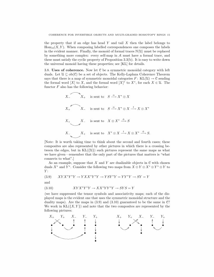
3.8. Uses of coherence. Now let C be a symmetric monoidal category with leftduals. Let U ⊆ ob(C) be a set of objects. The Kelly-Laplaza Coherence Theoremsays that there is a map of symmetric monoidal categories F : KL(U)→ C sendingthe formal word [X] to X, and the formal word [X]∗ to X∗, for each X ∈ U. Thefunctor F also has the following behavior:
X−##X+ is sent to S
α−→ X∗ ⊗X
X+ X−{{
is sent to Sα−→ X∗ ⊗X t−→ X ⊗X∗
X+ ;;X− is sent to X ⊗X∗ α−→ S
X− X+cc is sent to X∗ ⊗X t−→ X ⊗X∗ α−→ S.
[Note: It is worth taking time to think about the second and fourth cases; thesecomposites are also represented by other pictures in which there is a crossing be-tween the edges, but in KL({U}) such pictures represent the same maps as whatwe have given—remember that the only part of the pictures that matters is “whatconnects to what”.]
As an example, suppose that X and Y are dualizable objects in C with chosenduals X∗ and Y ∗. Consider the following two maps from X ⊗ Y ⊗X∗ ⊗ Y ∗ ⊗ Y toY :
XYX∗Y ∗Y → Y XX∗Y ∗Y → Y SY ∗Y = Y Y ∗Y → SY = Y(3.9)
and
XYX∗Y ∗Y → XX∗Y Y ∗Y → SY S = Y(3.10)
(we have suppressed the tensor symbols and associativity maps; each of the dis-played maps is the evident one that uses the symmetric monoidal structure and theduality maps). Are the maps in (3.9) and (3.10) guaranteed to be the same in C?We work in KL({X,Y }) and note that the two composites are represented by thefollowing pictures:
X+
""FFFFFY+
||xxxxx
X− Y− Y+
��
X+
��
Y+
##FFFFFX− Y− Y+
��•��
• BB•
OO
•
OO
•��
• BB•
<<xxxxx •��
•
OO
•[[
• 99 •
OO
•��
•
•

16 DANIEL DUGGER
The composite pictures are clearly not the same map in KL(U), and so there is noguarantee that the two maps are the same in C. They might be the same, but if sothis is an “accident”—it does not follow from the basic axioms.
As one more example, let us consider the following composite:
S = SSS // X∗XY ∗Y XX∗ // X∗Y ∗XXYX∗tX,X // X∗Y ∗XXYX∗
��S = SSS X∗XY ∗Y XX∗oo
Note that in the third map we have omitted the identity factors on either side ofthe tX,X , due to limitations of space. All of the other maps are the evident ones.We claim that the composite can be given a simpler description. Computing inKL({X,Y }) we get the following picture:
X•��•
$$HHHH
H •Y��•
""EEEEE •
||yyyyy
•X��
•
OO
•
;;vvvvv •$$HH
HHH •zzvvv
vv•��
•
OO
•
OO
•
OO
•zzvvv
vv•
""EEEEE •
||yyyyy
•
OO
•
OO
•[[ •
ddHHHHH•[[ • CC•
OO
This picture breaks up into two loops, one where the vertices are all labelled byX and the other where they are all labelled by Y . As a map from S to S inKL({X,Y }) this composite is therefore equal to tr(idX) ◦ tr(idY ) (note that theorder of composition does not matter, since Hom(S, S) is commutative). Since thisidentity holds in the universal example KL({X,Y }), it also holds in C.
Remark 3.11 (Traces in Kelly-Laplaza categories). Let w be an object in KL({U})and let f : w → w be a map. Then tr(f) is a map S → S in KL({U}). We leave itas an easy exercise to verify that tr(f) is represented by the following picture:
f
(where the picture representing f should be inserted into the blank box).
4. Invertible objects
In this section we review the notion of invertible object in a symmetric monoidalcategory, and establish some of their properties. For every invertible object X wedefine a basic commuter τX , which is an isomorphism τX : S → S such that τ2
X = 1.

COHERENCE FOR INVERTIBLE OBJECTS AND MULTI-GRADED HOMOTOPY RINGS 17
4.1. Prelude. Throughout this section (C,⊗, S) is a symmetric monoidal category.If u : S → S and g : A→ B then denote the composites
A ∼= S ⊗A u⊗g−→ S ⊗B ∼= B and A ∼= A⊗ S g⊗u−→ B ⊗ S ∼= B
by u ⊗ g and g ⊗u. We will sometimes omit the carat and just write u ⊗ g andg ⊗ u by abuse, but at other times it is useful to remember that u ⊗ g and u ⊗ gare somewhat different.
Lemma 4.2. Let u : S → S and g : A→ B. Then
u ⊗ g = (u ⊗ idB) ◦ g = g ◦ (u ⊗ idA) = g ⊗u.Proof. This is elementary, using that u ⊗ g = (idS ⊗g) ◦ (u ⊗ idA) = (u ⊗ idB) ◦(idS ⊗g) and similarly for g ⊗ u. �
Remark 4.3. The above lemma will often be used in the following way. Supposethat g : A→ B and f : B → C. Then multiple applications of the lemma give
(u ⊗ f) ◦ g = f ◦ (u ⊗ idB) ◦ g = f ◦ (u ⊗ g) = f ◦ g ◦ (u ⊗ idA) = u ⊗ (fg).
So we can move a u ⊗ (−) from anywhere inside a composite to anywhere else,including outside the composite.
Remark 4.4. Observe that for any object V in C we obtain a map of monoidsEnd(S)→ End(V ) given by u 7→ u ⊗ idV .
4.5. Invertible objects.
Definition 4.6. An object X in C is invertible if there exists a Y in C and anisomorphism α : S → Y ⊗X.
It is easy to prove that if such a Y exists then it is unique up to isomorphism.But to give an inverse for an object X, one must specify an object Y together withthe isomorphism α : Y ⊗ X → S. This map α is not uniquely determined by Y ,since one can clearly get a different α by composing with an automorphism of S.Note that if X and Z are invertible then clearly so is X ⊗ Z.
We will often use the following observation:
Proposition 4.7. If X is an invertible object in C then the canonical mapEnd(S) → End(X) is an isomorphism of monoids. More generally, for any ob-ject V of C the two maps End(V ) → End(V ⊗ X) and End(V ) → End(X ⊗ V )(obtained by tensoring with identity maps) are both isomorphisms.
Proof. Choose an inverse (Y, α) for X. The functor TX : C→ C given by Z 7→ Z⊗Xis an equivalence of categories, because an inverse is given byW 7→W⊗Y . Since TXis an equivalence, for any V in C the map End(V )→ End(TX(V )) is an isomorphismof monoids. A similar argument shows End(V )→ End(X⊗V ) to be an isomorphism(or use the twist map X ⊗ V ∼= V ⊗X).
When V = S one has TX(S) ∼= X via the unital isomorphism, and the compositeEnd(S)→ End(TX(S)) ∼= End(X) is readily checked to be the map of Remark 4.4.
�
When X is invertible it will be useful to have a description of the inverse tothe isomorphism End(S) → End(X). If (Y, α) is a choice of inverse for X andg : X → X, define DY (g) to be the composite
Sα−→ Y ⊗X id⊗g−→ Y ⊗X α−1
−→ S.

18 DANIEL DUGGER
An easy diagram chase shows that DY (u ⊗ idX) = u, for u ∈ End(S). SinceEnd(S)→ End(X) is an isomorphism this verifies that DY is the inverse, and so inparticular does not depend on the choice of (Y, α). From now on we will just writeD(g) rather than DY (g).
The homomorphism D : End(X) → End(S) is a bit like a trace, but it doesnot coincide with the standard trace that exists for dualizable objects as definedin Section 3.1 (see Remark 4.15 for an explicit example). The map D can alsobe regarded as something like a determinant—this analogy works well when C isa category of vector spaces or vector bundles, but of course in those cases thedeterminant and trace are indistinguishable on one-dimensional objects. In thepresent paper we will just call D(f) the “D-invariant” of the map f : X → X.Like a determinant, the D-invariant is multiplicative (being a homomorphism ofmonoids): that is, D(idX) = idS and D(fg) = D(f)D(g). Here are some furtherproperties of the D-invariant:
Lemma 4.8. Let X and Z be invertible objects.(a) Given a commutative diagram
X
f
��
q // Z
h
��X
q // Z
in which q is an isomorphism, one has D(f) = D(h).(b) If f : X → X, then D(idZ ⊗f) = D(f ⊗ idZ) = D(f).(c) If f : X → X and g : Z → Z then D(f ⊗ g) = D(f)D(g), where the product on
the right-hand-side is in the monoid End(S).
Proof. All of the parts are easy exercises. For (a) one uses the diagram
End(S) //
%%KKKKKKKKKEnd(X)
��End(Z)
where the vertical arrow sends a map f to qfq−1. One checks that the diagramcommutes using Remark 4.3, and then it follows at once that D(qfq−1) = D(f).
For (b) one looks at the composite End(S) → End(X) → End(X ⊗ Z). Bothmaps are isomorphisms, DX is the inverse of the first map, and DX⊗Z is the inverseof the composite; it follows at once that DX⊗Z(f ⊗ idZ) = D(f).
Finally, (c) follows from (b) and the fact that f ⊗ g = (f ⊗ idZ) ◦ (idX ⊗g). �
Remark 4.9. Let f : A → B and g : B → B, where B is invertible. The D-invariant of g is the unique map S → S satisfying g = D(g) ⊗ idB . We can thenwrite
gf = (D(g) ⊗ idB) ◦ f = f ◦ (D(g) ⊗ idA),using Remark 4.3 for the second equality. So automorphisms of invertible objectscan effectively be moved around inside a composition, by replacing them with theirD-invariant.

COHERENCE FOR INVERTIBLE OBJECTS AND MULTI-GRADED HOMOTOPY RINGS 19
4.10. The adjoint to α and the trace of a map. The following result showsthat an invertible object is left dualizable.
Proposition 4.11. Let X be an invertible object in C, with inverse (Y, α). Thenthere is a unique map α : X ⊗ Y → S with the property that the composite
X ∼= X ⊗ S id⊗α−→ X ⊗ (Y ⊗X) ∼= (X ⊗ Y )⊗X α⊗id−→ S ⊗X ∼= X
equals the identity. Moreover, α is an isomorphism and the composite
Y ∼= S ⊗ Y α⊗id−→ (Y ⊗X)⊗ Y ∼= Y ⊗ (X ⊗ Y ) id⊗α−→ Y ⊗ S ∼= Y
also equals the identity.
Remark 4.12. Note that one is tempted to assume that α equals the composite
X ⊗ Y t−→ Y ⊗X α−1
−→ S.(4.13)
This need not be the case. Let k be a field and let C = GrV ect±k be the categoryof Z-graded vector spaces with the usual tensor product, and with the twist mapthat involves signs. Let X = k[1], and Y = k[−1]. Let α : k → Y ⊗ X send 1 to1⊗1. Then α : X⊗Y → k must be the multiplication map, whereas the composite(4.13) sends a⊗ b to −ab.
Proof of Proposition 4.11. Let FX : C → C be given by FX(A) = A ⊗ X, and letFY : C → C be given by FY (A) = A ⊗ Y . These are an equivalence of categories.Consider the chain of functions
C(X ⊗ Y, S) FX−→ C((X ⊗ Y )⊗X,S ⊗X)γ∗−→ C(X,S ⊗X)
∼=−→ C(X,X)
where γ : X → (X ⊗ Y )⊗X is the composite
X∼=−→ X ⊗ S id⊗α−→ X ⊗ (Y ⊗X)
∼=−→ (X ⊗ Y )⊗X.Since γ is an isomorphism, γ∗ is a bijection. Likewise, the map labelled FX is abijection because FX is part of an equivalence of categories. So the whole compositeis a bijection, and we let α be the unique map whose image is the identity idX .This justifies the first claim in the statement of the proposition.
To see that α is an isomorphism, consider again the first composite in the state-ment. All the maps other than α ⊗ id are known to be isomorphisms, so we canconclude the same for α⊗id = FX(α). As FX is part of an equivalence of categories,it must be that α was an isomorphism itself.
Finally, let f : Y → Y be the second composite in the statement. We have acommutative diagram
X ⊗ Y
id ))TTTTTTTTTTTTTTTid⊗α⊗id // X ⊗ Y ⊗X ⊗ Y
α⊗id⊗ id
��
id⊗ id⊗α // X ⊗ Y ⊗ S∼= // X ⊗ Y
�
X ⊗ Y α // S,
where we have left off several associativity isomorphisms. The triangle commutesby the defining property of α, and the composite across the top row is idX ⊗f . Sothe diagram shows that α ◦ (idX ⊗f) = α. As α is an isomorphism we concludethat idX ⊗f = idX⊗Y . From this it follows that f = idY , by Proposition 4.7. �

20 DANIEL DUGGER
Suppose that X is invertible and f : X → X. Since X is left dualizable we maytake the trace, obtaining tr(f) : S → S. Recall that we have another way to obtaina self-map of S, namely the D-invariant D(f). These are connected by the followingformula:
Proposition 4.14. Let X be an invertible object and let f : X → X. Then onehas tr(idX) ·D(f) = tr(f).
Proof. The composite tr(idX) ·D(f) is
Sα−→ Y ⊗X id⊗f−→ Y ⊗X α−1
−→ Sα−→ Y ⊗X id−→ Y ⊗X t−→ X ⊗ Y α−→ S.
The terms in the middle cancel and we obtain the definition of tr(f). �
Remark 4.15. Consider again the example GrV ect±k from Remark 4.12, with X,Y , and α as described there. Then tr(idX) = −1, but of course D(idX) = 1. Sothis gives an example where the trace and D-invariant are distinct.
Our next major goal will be to prove that whenX is invertible one has tr(idX)2 =idS . This is an important property of invertible objects, but unfortunately we havenot been able to find a direct, simple-minded proof. We will instead deduce theresult from a cyclic permutation property, which a priori feels somewhat deeper.
4.16. Automorphisms of invertible objects induced from permutations.Let x1, . . . , xn be formal variables and let w be any tensor word in the xi’s withthe property that each xi appears exactly once. For instance, if n = 3 we mighthave w = (x1⊗x3)⊗x2. We can associate to w a functor Fw : Cn → C which plugsin objects for the variables xi. For objects X1, . . . , Xn in C write w(X1, . . . , Xn) asshorthand for Fw(X1, . . . , Xn), and write w(X) as shorthand for Fw(X,X, . . . ,X).
If σ is a permutation of {1, . . . , n}, we let wσ denote the word in which xi hasbeen replaced by xσ(i). So we can write
Fwσ(X1, . . . , Xn) = Fw(σ · (X1, . . . , Xn)) = Fw(Xσ(1), Xσ(2), . . . , Xσ(n)).
By MacLane’s coherence theorem [M, Theorem XI.1.1] there is a unique naturaltransformation Fw → Fwσ obtained by composing associativity and commutativityisomorphisms. If X is an object in C, we can evaluate this natural transformation atthe tuple (X,X, . . . ,X) and thereby obtain an automorphism φw,σ : w(X)→ w(X).In this way we obtain a function φw : Σn → Aut(w(X)), which is readily checkedto be a homomorphism.
The following result is from [V, Discussion preceding Theorem 4.3]:
Lemma 4.17. Let X be an invertible object in C. Then for any tensor word w inn variables, and any even permutation σ in Σn, the map φw,σ : w(X) → w(X) isequal to the identity. In particular, the composite map
(X ⊗X)⊗X tX⊗X,X−→ X ⊗ (X ⊗X) a−→ (X ⊗X)⊗Xis equal to the identity. (Note that this composite map is an instance of the canonicalmap (A⊗B)⊗ C → C ⊗ (A⊗B), i.e. the cyclic permutation map).
Proof. Since X is invertible, so is w(X). Hence Aut(w(X)) is abelian by Propo-sition 4.7 and Lemma 3.4. This means the homomorphism φw : Σn → Aut(w(X))kills the commutator subgroup of Σn, which is the alternating group An. �
We can now obtain our goal:
COHERENCE FOR INVERTIBLE OBJECTS AND MULTI-GRADED HOMOTOPY RINGS 21
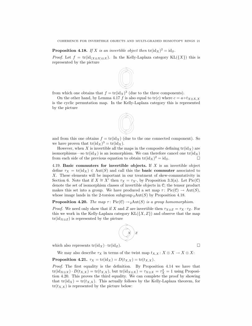
Proposition 4.18. If X is an invertible object then tr(idX)2 = idS.
Proof. Let f = tr(id(X⊗X)⊗X). In the Kelly-Laplaza category KL({X}) this isrepresented by the picture
from which one obtains that f = tr(idX)3 (due to the three components).On the other hand, by Lemma 4.17 f is also equal to tr(c) where c = a◦ tX⊗X,X
is the cyclic permutation map. In the Kelly-Laplaza category this is representedby the picture
and from this one obtains f = tr(idX) (due to the one connected component). Sowe have proven that tr(idX)3 = tr(idX).
However, when X is invertible all the maps in the composite defining tr(idX) areisomorphisms—so tr(idX) is an isomorphism. We can therefore cancel one tr(idX)from each side of the previous equation to obtain tr(idX)2 = idS . �
4.19. Basic commuters for invertible objects. If X is an invertible objectdefine τX = tr(idX) ∈ Aut(S) and call this the basic commuter associated toX. These elements will be important in our treatment of skew-commutativity inSection 6. Note that if X ∼= X ′ then τX = τX′ , by Proposition 3.3(a). Let Pic(C)denote the set of isomorphism classes of invertible objects in C; the tensor productmakes this set into a group. We have produced a set map τ : Pic(C) → Aut(S),whose image lands in the 2-torsion subgroup 2Aut(S) by Proposition 4.18.
Proposition 4.20. The map τ : Pic(C)→2Aut(S) is a group homomorphism.
Proof. We need only show that if X and Z are invertible then τX⊗Z = τX · τZ . Forthis we work in the Kelly-Laplaza category KL({X,Z}) and observe that the maptr(idX⊗Z) is represented by the picture
X Z
which also represents tr(idX) · tr(idZ). �
We may also describe τX in terms of the twist map tX,X : X ⊗X → X ⊗X:
Proposition 4.21. τX = tr(idX) = D(tX,X) = tr(tX,X).
Proof. The first equality is the definition. By Proposition 4.14 we have thattr(idX⊗X) ·D(tX,X) = tr(tX,X), but tr(idX⊗X) = τX⊗X = τ2
X = 1 using Proposi-tion 4.20. This proves the third equality. We can complete the proof by showingthat tr(idX) = tr(tX,X). This actually follows by the Kelly-Laplaza theorem, fortr(tX,X) is represented by the picture below:

22 DANIEL DUGGER
Because there is only one connected component, this also represents tr(idX). �
5. Coherence for invertible objects
In this section we prove our main coherence theorems for invertible objects ina symmetric monoidal category. We deduce these as consequences of the Kelly-Laplaza theorem.
Let (C,⊗, S) be a symmetric monoidal category and let X be an invertible objectwith inverse (X∗, α). Recall that tr(idX) is defined to be the composite
Sα−→ X∗ ⊗X t−→ X ⊗X∗ α−→ S.
Every map in this composite is an isomorphism, so we can write
α−1 = tr(idX)−1 ◦ (αt) = tr(idX) ◦ (αt) = tr(idX) ⊗ (αt)
where in the second equality we have used that tr(idX)2 = idS (see Proposi-tion 4.18). Similarly, we have
α−1 = tr(idX) ⊗ (tα).
Let Cinv be the full subcategory of invertible objects. Then Cinv is a symmetricmonoidal category with left duals. We will deduce our desired coherence theoremsfor invertible objects from Kelly-Laplaza coherence applied to Cinv.
We saw in Section 3 that maps in a Kelly-Laplaza category can be representedby pictures consisting of certain kinds of directed curves in the plane. These curvesare very simple: every crossing is a standard “X”-crossing, and every place wherethere is a horizontal tangent line is either a local minimum or local maximum withrespect to the y-coordinate (i.e., a cup or cap)—we will call these cups and capsthe critical points of the curve.
5.1. Coherence without self-twists.
Proof of Theorem 1.6. Let us use the term “acceptable” for formal composites ofthe type considered in the statement of the proposition. Suppose there were twoacceptable formal composites f, g : w1 → w2 that yielded different maps in C. Thenthe formal composite g−1f : w1 → w1 would yield a map in C different from theidentity. So it suffices to prove the proposition in the case w1 = w2 and g = id.
Suppose f : w1 → w1 is an acceptable formal composite such that f(C) 6= id.Let w∗1 be the formal inverse of the word w1, and choose any acceptable formalcomposite h : S → w∗1 ⊗ w1. Consider the formal composite
Sh−→ w∗1 ⊗ w1
id⊗f−→ w∗1 ⊗ w1h−1
−→ S.
Since f(C) 6= id Proposition 4.7 shows that the map id⊗f also does not give theidentity in C, and from this it follows that the above composite does not give theidentity either. So it suffices to prove the proposition in the case w1 = w2 = S andg = id.
Let n1 be the number of α−1 maps that appear in f , and let n2 be the number ofα−1 maps that appear. Let n = n1 + n2. Let F be the formal composite in which

COHERENCE FOR INVERTIBLE OBJECTS AND MULTI-GRADED HOMOTOPY RINGS 23
every α−1 has been replaced with αt and every α−1 has been replaced with tα.Using Remark 4.3, the identities α−1 = tr(idX) ⊗ (αt) and α−1 = tr(idX) ⊗ (tα)show that f(C) = tr(idX)n ⊗F (C).
The reason for introducing F is that it only involves maps that exist for dualizableobjects, rather than invertible ones. So we may consider F as a composite in thecategory Kelly-Laplaza category KL({X}). The assumption that f was acceptableimplies that F can be represented by the disjoint union of simple closed curves; forexample, one of the components might look like this:
Let us be clear about why this works. The assumption that the formal composite fis acceptable guarantees that the only twist maps that appear in F come togetherwith an α or α. In terms of the pictures, each of these twists can be eliminated; tosee this, recall how the pictures work:
•��• = α, • AA• = α,
•��•
������
���
= = tα,
• •��
• •
[[6666666
• •
������
���
= = αt.
• •ZZ • DD•
[[7777777
The twists in F only appear in conjunction with a cup or cap, and so they can allbe depicted by an untwisted cup or cap going in the opposite direction.
Now we come to the crux of the matter. For the moment assume that the picturefor F only contains one component, for simplicity. In this simple closed curve, everyα or α appears as a right-pointing arrow on a cup or cap. Likewise, every tα or αtappears as a left-pointing arrow on a cup or cap. So the number of left-pointingarrows in our simple closed curve is n1 + n2 = n. But elementary topology showsthat in a (nice enough) directed, simple, closed curve the number of left-pointingcritical points must always be odd (the same is true for the number of right-pointingcritical points, of course). So n is odd.
In the category KL({(X}) we know that a simple closed curve as above is equalto tr(idX). So when F is evaluated in C it also gives this trace. Putting everythingtogether, we find that f(C) = tr(idX)n ◦ F (C) = tr(idX)n ◦ tr(idX) = tr(idX)n+1.

24 DANIEL DUGGER
Given that n is odd, this just equals the identity (using Proposition 4.18). Thiscompletes the proof for the case that the picture for F has only one component.
For the multi-component case we observe that in KL({X}) the map F is thecomposition of the maps represented by each individual component; by what hasalready been argued, F (C) is a composition of identity maps and hence equal tothe identity. �
Proof of Theorem 1.13. This is essentially the same as the proof of Theorem 1.6,except we use the Kelly-Laplaza category KL({X1, . . . , Xn}). Note that the exis-tence part of the theorem is obvious; the work lies in showing uniqueness of theisomorphism. For this one reduces, just as in Theorem 1.6, to the case of a com-posite f that starts and ends with S and is of the type specified in the statementof the theorem.
The composite f is then replaced by a corresponding formal composite F inKL({X1, . . . , Xn}). The picture for F is a collection of simple, closed curves in theplane, each labelled by one of the Xi’s, which are allowed to intersect each otherin double points. The Kelly-Laplaza theorem identifies F with the composite ofthe maps whose pictures correspond to each closed curve. In this way one reducesto the one-variable case handled by Theorem 1.6, to conclude that f must be theidentity. �
5.2. Coherence with self-twists.
Proof of Theorem 1.10. The proof proceeds along the same lines as that of Theo-rem 1.6. One immediately reduces to the case w1 = w2 = S, g = id, and wherethe parity of f is even. Just as before, we replace f by a corresponding formalcomposite F in the Kelly-Laplaza category KL({X}). We have
f(C) = tr(idX)n ◦ F (C),
where the integer n is the same as in the proof of Theorem 1.6.The picture corresponding to F is no longer a union of simple curves as it was
in the proof of Theorem 1.6. Rather, it is a union of oriented, closed curves thatmay contain double points of self-intersection. For pedagogical purposes let us firstdeal with the case where the picture contains a single closed curve, for example asfollows:
It is easy to prove that in such an oriented curve one has
(# of left-pointing critical points) + (# of double points) ≡ 1 mod 2.(5.3)
Indeed, let L denote the number on the left of the congruence. Imagine taking aclosed loop of string—an unknot—and laying it on top of the plane containing our

COHERENCE FOR INVERTIBLE OBJECTS AND MULTI-GRADED HOMOTOPY RINGS 25
oriented curve, in such a way that the string exactly covers the curve. This gives usan oriented knot diagram which is similar to our original picture but in which everydouble-point has been changed to an over- or under-crossing. One readily checksthat the parity of the number L is unchanged under the Reidemeister moves. Sinceour knot diagram is equivalent to the unknot, this says that the parity of L is thesame as the corresponding number for an oriented circle. But a circle clearly givesL = 1.
The number of left-pointing critical points in the picture for F is just the numbern. Likewise, the number of double points in the picture is the parity of the formalcomposite f , which we have assumed to be even. So (5.3) tells us that n is odd.
The Kelly-Laplaza theorem implies that F (C) = tr(idX). So f(C) = tr(idX)n+1.Since n + 1 is even tr(idX)n+1 = idS by Proposition 4.18, and this completes theproof in the present case (where the picture for F contains one closed curve).
For the general case we have F (C) = tr(idX)e where e is the number of closedcurves in the picture. The analog of (5.3)—whose proof is the same as before—becomes
(# of left-pointing critical points) + (# of double points) ≡ e mod 2.(5.4)
We then obtain f(C) = tr(idX)n+e, and (5.4) yields that n+ e is even. So again wehave f(C) = idS , as desired. �
Proof of Theorem 1.14. This is a straightforward generalization of the proof of The-orem 1.10, in the same way that Theorem 1.13 generalized Theorem 1.6. The mainpoint is that a map from S to S in KL({X1, . . . , Xn}) is represented by a collectionof closed curves, each of which is labelled by one of the Xi’s. The Kelly-Laplazatheorem identifies such a map with the composite of the maps obtained by consid-ering each closed curve separately. The i-parity of our formal composite representsthe number of double points in the curves labelled by Xi. The hypothesis that eachof these parities is even guarantees, just as in the proof of Theorem 1.13, that thespecified map in KL({X1, . . . , Xn}) is the identity. �
6. The main applications: Zn-graded rings of maps
Assume that (C,⊗, S) is an additive category with a symmetric monoidal struc-ture, where the tensor product is an additive functor in each variable. In thissection we investigate Zn-graded groups of maps in C.
Suppose X1, . . . , Xn ∈ C are invertible objects, and let (X∗i , αi) be a specific
choice of inverse forXi. Recall the definition ofXa for every a ∈ Zn, from Section 1.For every a, b ∈ Zn there is a canonical isomorphism
φa,b : Xa ⊗Xb ∼=−→ Xa+b
specfied by Theorem 1.13. The uniqueness part of that proposition guarantees thatthe pentagonal diagrams (2.1) all commute, and that for a, b ∈ Nn these φa,b’scoincide with the ones defined in Section 2.
For any W ∈ C define π∗(W ) to be the Zn-graded abelian group
π∗(W ) = ⊕a∈ZnC(Xa,W ).
Suppose that U , V , and W are objects and that there is a pairing U ⊗ V → W .The maps φa,b allow us to define a Zn-graded pairing π∗(U)⊗ π∗(V )→ π∗(W ) as

26 DANIEL DUGGER
follows. Suppose f : Xa → U and g : Xb → V . Define the product f · g to be thecomposite
Xa+bφ−1
a,b−→ Xa ⊗Xb f⊗g−→ U ⊗ V −→W.
Proposition 6.1. Let U be a monoid with respect to ⊗.(a) π∗(U) is a Zn-graded ring (associative and unital).(b) If V is a left (resp. right) module over U then π∗(V ) is a left (resp. right)
module over π∗(U).(c) If U is a commutative monoid then π0(U) is central in π∗(U).
Proof. The proofs of (a) and (b) are the same: distributivity is automatic, andassociativity follows from the commutativity of the diagram (2.1) involving theφa,b’s. The unit conditions follow as in the proof of Proposition 2.3.
For (c), let f : Xa → U and g : S → U . The following diagram is commutative:
Xa //
##HHHHHHHH Xa ⊗ S
t
��
f⊗g // U ⊗ U
t
��
µ// U
S ⊗Xa g⊗f // U ⊗ Uµ
<<yyyyyyyyy
The composite across the top is f · g, and the composite across the bottom is g · f .Commutativity of the diagram shows these are equal. �
6.2. Representation of elements in π∗(S) by maps in C. Let w1 and w2 betwo tensor words in the symbols X±1
i , and suppose that f : w1 → w2 is a map.Theorem 1.13 gives canonical isomorphisms Xa → w1 and Xb → w2 for uniquea, b ∈ Zn. From now on we will denote all canonical isomorphisms provided byTheorem 1.13 by φ. (A consequence of this is that a canonical map and its inverse—which is also canonical—are sometimes both denoted by φ; in practice this doesnot lead to much confusion, though.) Let 〈f〉 denote the composite
Xa φ−→ w1f−→ w2
φ−→ Xb.
There are two evident ways to obtain an element of π∗(S) from 〈f〉. Let [f ]r ∈πa−b(S) be the composite
Xa−b φ−→ X−b ⊗Xa id⊗〈f〉−→ X−b ⊗Xb φ−→ S.
and let [f ]l ∈ πa−b(S) be the composite
Xa−b φ−→ Xa ⊗X−b 〈f〉⊗id−→ Xb ⊗X−b φ−→ S.
In general one must be careful, as [f ]r and [f ]l need not be the same element. Wewill give a precise formula for relating them in Proposition 6.11 below, but it willtake some work to build up to this. We start with some simple observations:
Proposition 6.3. Let w1, w2, and w3 be three tensor words that are formallyisomorphic to Xa, Xb, and Xc, respectively. Let f : w1 → w2 and g : w2 → w3.(a) [idw3 ⊗f ]r = [f ]r and [f ⊗ idw3 ]l = [f ]l,(b) [gf ]r = [g]r · [f ]r.

COHERENCE FOR INVERTIBLE OBJECTS AND MULTI-GRADED HOMOTOPY RINGS 27
Proof. For part (a) first note that 〈idw3 ⊗f〉 = idc⊗〈f〉, by an easy argument.Next use the following diagram, where we have suppressed some tensor signs fortypograhical reasons:
X−b−cXa+cφ // X−b−cXcXa
φ⊗id
��
1⊗1⊗〈f〉// X−b−cXcXb
φ⊗id
��
id⊗φ // X−b−cXb+c
φ
��Xa−b
φ
OO
φ // X−bXa1⊗〈f〉 // X−bXb
φ // S.
The three squares are readily checked to commute; in the case of the outer onesthis is by Theorem 1.13. The composite from Xa−b to S across the ‘top’ of thediagram is [idw3 ⊗f ]r, and the composite across the bottom is [f ]r. The argumentshowing [f ⊗ idw3 ]l = [f ]l is entirely similar.
For (b) we first examine the commutative diagram
Xa−c φ1 // Xb−c ⊗Xa−bid⊗[f ]r //
[g]r⊗[f ]r ((QQQQQQQQQQQQ Xb−c ⊗ Sφ2 //
[g]r⊗id
��
Xb−c
[g]r
��S ⊗ S // S.
Let H = φ2 ◦ (id⊗[f ]r) ◦ φ1. The composite across the ‘bottom’ of the diagram is[g]r · [f ]r, so we have [g]r · [f ]r = [g]r ◦H.
Next consider the following diagram:
Xa−c φ //
φ1
��
X−cXaid⊗〈f〉 // X−cXb
id⊗〈g〉 // X−cXc φ // S
Xb−cXa−b id⊗φ // Xb−cX−bXa
φ⊗id
OO
1⊗1⊗〈f〉// Xb−cX−bXb
φ⊗id
OO
id⊗φ // Xb−cSφ2
// Xb−c
[g]r
OO
φ
jjVVVVVVVVVVVVVVVVVVVVVVV
All of the regions of the diagram commute, in two cases by Theorem 1.13. Thecomposite across the top row is [gf ]r. The composite across the bottom edge fromXa−c to Xb−c is the map H. So the diagram shows that [gf ]r = [g]r ◦H, and thelatter equals [g]r · [f ]r by the preceding paragraph. �
Remark 6.4. It is informative to check that the argument for part (b) of Propo-sition 6.3 does not dualize to prove [gf ]l = [g]l · [f ]l. The reason comes down tothe fact that the formula g⊗ f = (g⊗ id) ◦ (id⊗f) has the identity tensored on theleft side of the f . The dual argument shows [gf ]l = [f ]l · [g]l, although we will notneed this fact.
Our next task is to focus on the case where f : w1 → w2 and w1∼= w2
∼= Xa.Note that in this case 〈f〉 is a map Xa → Xa and so we also have the invariantsD(〈f〉) and tr(〈f〉), which like [f ]l and [f ]r are elements of π0(S). The followingresult gives the relation between all of these constructions:
Proposition 6.5. Let w1 and w2 be two words that are formally isomorphic toXa, for a ∈ Zn. Let f : w1 → w2 be a map.(a) [f ]r = [f ]l = D(〈f〉), and tr(〈f〉) = D(f) · tr(idXa).(b) [idc⊗f ]r = [f ⊗ idc]r = [f ]r, for any c ∈ Zn.

28 DANIEL DUGGER
(c) For a canonical isomorphism φ : w1 → w2 (as provided by Theorem 1.13) onehas [φ]r = idS.
Before giving the proof let us introduce one more important definition. Fora, b ∈ Zn we have the twist map ta,b : Xa⊗Xb → Xb⊗Xa. We write Ta,b = 〈ta,b〉,which is a map Xa+b → Xa+b. It is easy to check that Ta,b ◦ Tb,a = id. Note thatTa,−a is a map S → S.
Proof of Proposition 6.5. For (a) we consider the following diagram:
S
$$HHHH
HHHH
HH// X−a ⊗Xa //
t−a,a
��
X−a ⊗ w1
id⊗f //
t
��
X−a ⊗ w2//
t
��
X−a ⊗Xa
t−a,a
��
// S
Xa ⊗X−a // w1 ⊗X−a f⊗id // w2 ⊗X−a // Xa ⊗X−a
::vvvvvvvvvv
where all unlabelled maps are canonical isomorphisms (i.e., they should be labelledwith φ). The three squares are commutative, but the triangles on the two ends arenot; the automorphism of S obtained by moving around one of these triangles iseither Ta,−a or T−a,a, depending on which direction the composite is taken. Thecomposite across the top of the diagram is [f ]r and the composite across the bottomis [f ]l. The diagram thus yields the formula
[f ]r = Ta,−a ◦ [f ]l ◦ T−a,a.But this formula takes place in the monoid End(S), which is commutative by Propo-sition 4.7. So we obtain [f ]r = [f ]l ◦ Ta,−a ◦ T−a,a = [f ]l ◦ idS = [f ]l.
Next consider the diagram
S ⊗Xa
φ
��
φ⊗id // Xa ⊗X−a ⊗Xaφ⊗id⊗ id//
vvnnnnnnnnnnnnw1 ⊗X−a ⊗Xaf⊗id⊗ id//
uukkkkkkkkkkkkkkw2 ⊗X−a ⊗Xa
uukkkkkkkkkkkkkkφ⊗id⊗ id
��Xa ⊗ S
φ⊗id// w1 ⊗ S
f⊗id// w2 ⊗ S
φ⊗id
��
Xa ⊗X−a ⊗Xa
φ⊗id⊗ id
��uukkkkkkkkkkkkkk
Xa ⊗ Sφ
// S ⊗Xa.
The diagonal maps are all equal to the identity on the left tensor factor and thecanonical isomorphism φ : Xa ⊗ X−a → S on the other two factors. All of the‘squares’ obviously commute in the diagram, and the triangles on the two endscommute by Theorem 1.13 since all the maps are canonical isomorphisms. Thecomposition across the ‘top’ of the diagram equals [f ]l ⊗ idXa . Condensing thediagram to its outer rim yields the commutative square
S ⊗Xa [f ]l⊗id//
φ
��
S ⊗Xa
φ
��Xa ⊗ S
〈f〉⊗idS// Xa ⊗ S.
By Lemma 4.8(a) the top and bottom maps have the same D-invariant, and theD-invariant of the bottom map is also that of 〈f〉 (using the unital isomorphism).Finally, D([f ]l ⊗ id) = D([f ]l) = [f ]l by Lemma 4.8(b). This ends the proof of (a).
COHERENCE FOR INVERTIBLE OBJECTS AND MULTI-GRADED HOMOTOPY RINGS 29
Part (b) follows immediately from (a) and Proposition 6.3(a). Part (c) is aconsequence of coherence: the composite
Xa φ1−→ w1φ−→ w2
φ2−→ Xa
is a canonical map and must therefore equal the identity by Theorem 1.13. So〈φ〉 = idXa and [φ]r = D(idXa) = idS . �
The elements Ta,b ∈ Aut(S) are, of course, ubiquitous in calculations. We define
τa,b = [ta,b]l = [ta,b]r = D(Ta,b) ∈ π0(S),
where the second two equalities are by Proposition 6.5. Recall that we have thebasic commuters τi = tr(idXi
) ∈ π0(S) and these satisfy τ2i = 1 by Proposition 4.18.
Recall as well that τi = D(tXi,Xi) by Proposition 4.21. If e1, . . . , en is the standardbasis for Zn then this just says that τi = τei,ei . Let us also point out that if i 6= jthen τei,ej = idS ; in fact Tei,ej is the composite
Xei+ejφ−→ Xi ⊗Xj
tXi,Xj−→ Xj ⊗Xiφ−→ Xei+ej
and this equals the identity map either by Theorem 1.14 or by just looking at thedefinitions. Quite generally, we can express all of the elements τa,b in terms of thebasic commuters:
Proposition 6.6. For all a, b ∈ Zn one has τa,b = τ(a1b1)1 · · · τ (anbn)
n .
Proof. Recall that Ta,b is the composite Xa+b φ−→ Xa⊗Xb ta,b−→ Xb⊗Xa φ−→ Xa+b.Observe that we can also obtain this map as a long composite
Xa+b → w1 → w2 → · · · → wN → Xa+b(6.7)
where each wk is a tensor word in the X±1i ’s and each map is either
(1) a canonical isomorphism φ (as provided by Theorem 1.13),(2) a tensor product of tXi,Xi
with identity maps,(3) a tensor product of tXi,X
−1i
with identity maps, or(4) a tensor product of tX−1
i ,X−1i
with identity maps.
In the ‘standard’ way to obtain such a composite the number of transpositionsof types (2)–(4) will be |aibi|, for any chosen value of i. Let f : S → S be themap
∏i τ
(aibi)i , noting that only the parity of aibi matters in the exponent since
τ2i = idS . Consider the composite
Xa φ−→ S ⊗Xa f⊗id−→ S ⊗Xa φ−→ Xa.(6.8)
It follows from Theorem 1.14 that the composites in (6.7) and (6.8) are the same,because by construction they have the same i-parity for every i. Consequently,the D-invariant of the two composites is the same. But the D-invariant of (6.8) ismanifestly equal to the map f . We have thus proven that f = D(Ta,b) = τa,b. �
Remark 6.9. As a consequence of Proposition 6.6 and the fact that τ2i = 1 note
that we have τa,bτa,c = τa,b+c = τa,b−c. Likewise, τa,b = τ−a,b = τb,a. Identitiessuch as these will often be used.
Before proceeding further we need a lemma, which is easy but worth recording:

30 DANIEL DUGGER
Lemma 6.10. Consider composable maps Xa f−→ Xa g−→ Sh−→ S. Then as
elements of π∗(S) one has hg = h · g = g · h and gf = g ·D(f). More generally, wecan write hgf = h · g ·D(f) = g · h ·D(f).
Proof. We have already seen that h · g = g ·h, in Proposition 2.3. The identificatonof these with the composite hg is easy. For the second identity we have
g ◦ f = g ◦ (idX ⊗D(f)) = g ⊗D(f) = g ·D(f)
where the second equality is from Lemma 4.2 and the third equality follows from thedefinitions. Finally, the identity for hfg is a consequence of the previous identities.
�
Now we can move on to the study of [f ]r and [f ]l for general maps f .
Proposition 6.11. Let w1 and w2 be two tensor words, where w1 is formallyisomorphic to Xa and w2 is formally isomorphic to Xb. Let f : w1 → w2, and letc ∈ Zn. Write idc for idXc .(a) [f ]r = [f ]l · τb,a−b(b) [idc⊗f ]r = [f ]r(c) [f ⊗ idc]r = [f ]r · τa−b,c(d) [f ⊗ idc]l = [f ]l(e) [idc⊗f ]l = [f ]l · τa−b,c(f) If g : w2 → w3 where w3
∼= Xc, then [gf ]r = [g]r · [f ]r and likewise [gf ]l =[g]l · [f ]l · τa−b,c−d.
(g) Let g : w′1 → w′2 where w′1 ∼= Xc and w′2 ∼= Xd. Then
[f ⊗ g]r = [f ]r · [g]r · τa−b,d = [g]r · [f ]r · τa−b,cand
[f ⊗ g]l = [f ]l · [g]l · τb,c−d = [g]l · [f ]l · τa,c−d.
Proof of Proposition 6.11. Note first that parts (b), (d), and the first part of (f)were already proven in Proposition 6.3; they are only restated here for ease ofreference. Note also that parts (c), (e), and the second part of (f) are formalconsequences of the aforementioned results, using (a). So most everything followsfrom (a).
To prove (a) we consider the usual diagram
Xa−b φ //
φ %%KKKKKKKKK X−b ⊗Xa
t−b,a
��
id⊗〈f〉// X−b ⊗Xb
t−b,b
��
φ // S
Xa ⊗X−b 〈f〉⊗id// Xb ⊗X−b.
φ
::vvvvvvvvvv
The square commutes but the triangles do not; the composite across the top is [f ]rand the composite across the bottom is [f ]l. The diagram yields the formula
[f ]r = Tb,−b ◦ [f ]l ◦ T−b,a.From Lemma 6.10 we get that in π∗(S) one has the formula
[f ]r = [f ]l · Tb,−b · τ−b,a = [f ]l · τb,−b · τ−b,a = [f ]l · τa−b,b(using Remark 6.9 for the final equality).
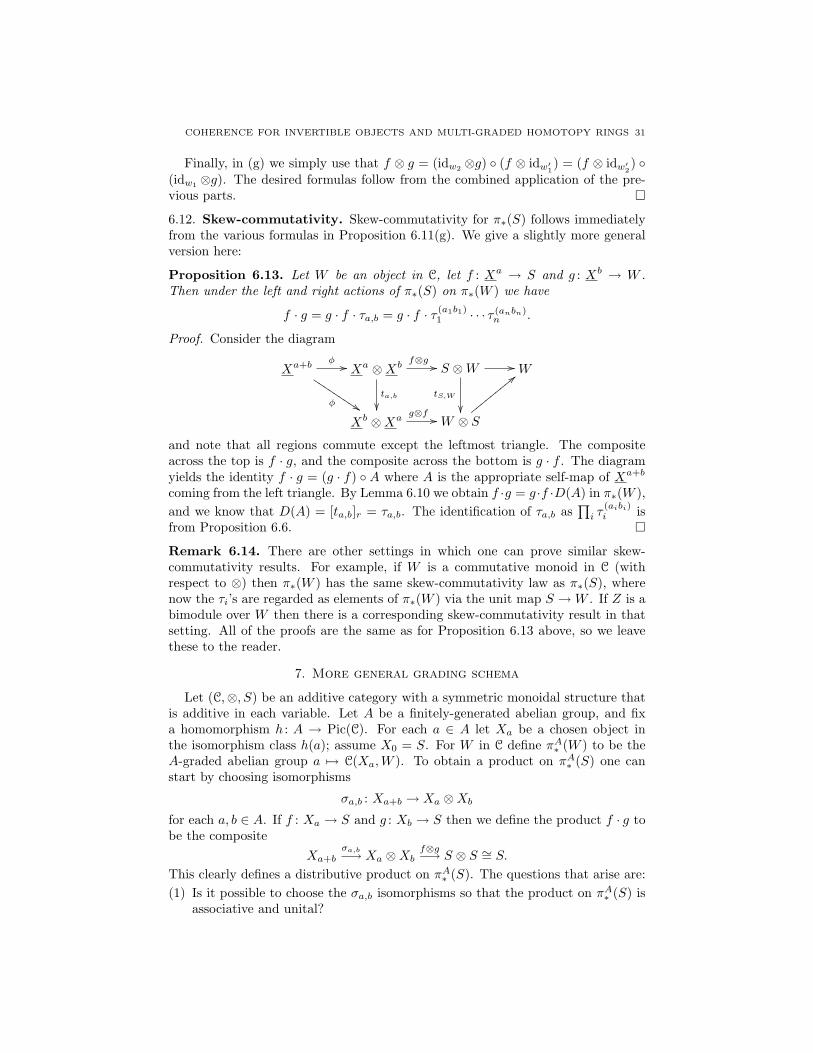
COHERENCE FOR INVERTIBLE OBJECTS AND MULTI-GRADED HOMOTOPY RINGS 31
Finally, in (g) we simply use that f ⊗ g = (idw2 ⊗g) ◦ (f ⊗ idw′1) = (f ⊗ idw′2) ◦(idw1 ⊗g). The desired formulas follow from the combined application of the pre-vious parts. �
6.12. Skew-commutativity. Skew-commutativity for π∗(S) follows immediatelyfrom the various formulas in Proposition 6.11(g). We give a slightly more generalversion here:
Proposition 6.13. Let W be an object in C, let f : Xa → S and g : Xb → W .Then under the left and right actions of π∗(S) on π∗(W ) we have
f · g = g · f · τa,b = g · f · τ (a1b1)1 · · · τ (anbn)
n .
Proof. Consider the diagram
Xa+bφ //
φ $$JJJJJJJJJ Xa ⊗Xb
ta,b
��
f⊗g // S ⊗W //
tS,W
��
W
Xb ⊗Xag⊗f // W ⊗ S
<<yyyyyyyyy
and note that all regions commute except the leftmost triangle. The compositeacross the top is f · g, and the composite across the bottom is g · f . The diagramyields the identity f · g = (g · f) ◦ A where A is the appropriate self-map of Xa+b
coming from the left triangle. By Lemma 6.10 we obtain f ·g = g ·f ·D(A) in π∗(W ),and we know that D(A) = [ta,b]r = τa,b. The identification of τa,b as
∏i τ
(aibi)i is
from Proposition 6.6. �
Remark 6.14. There are other settings in which one can prove similar skew-commutativity results. For example, if W is a commutative monoid in C (withrespect to ⊗) then π∗(W ) has the same skew-commutativity law as π∗(S), wherenow the τi’s are regarded as elements of π∗(W ) via the unit map S →W . If Z is abimodule over W then there is a corresponding skew-commutativity result in thatsetting. All of the proofs are the same as for Proposition 6.13 above, so we leavethese to the reader.
7. More general grading schema
Let (C,⊗, S) be an additive category with a symmetric monoidal structure thatis additive in each variable. Let A be a finitely-generated abelian group, and fixa homomorphism h : A → Pic(C). For each a ∈ A let Xa be a chosen object inthe isomorphism class h(a); assume X0 = S. For W in C define πA∗ (W ) to be theA-graded abelian group a 7→ C(Xa,W ). To obtain a product on πA∗ (S) one canstart by choosing isomorphisms
σa,b : Xa+b → Xa ⊗Xb
for each a, b ∈ A. If f : Xa → S and g : Xb → S then we define the product f · g tobe the composite
Xa+bσa,b−→ Xa ⊗Xb
f⊗g−→ S ⊗ S ∼= S.
This clearly defines a distributive product on πA∗ (S). The questions that arise are:(1) Is it possible to choose the σa,b isomorphisms so that the product on πA∗ (S) is
associative and unital?

32 DANIEL DUGGER
(2) If there are multiple ways to accomplish (1), do they give rise to isomorphicrings? That is, is the ring structure on πA∗ (S) in some sense canonical?
Note that in Section 6 we proved that the answer to (1) is yes in the case whenA is free. The construction depended on choosing a free basis e1, . . . , en for A andthen fixing a specific choice of isomorphism αi : S → X−ei ⊗Xei for each i; so theconstruction was certainly not canonical.
We will see below that the answer to (1) is yes in general, but the answer to (2)is no. In fact, the set of isomorphism classes of ring structures obtained in this wayis parameterized by the cohomology group H2(A; Aut(S)). Much of the materialbehind this story seems to be standard, but we were unable to find an adequatereference (the introduction to the paper [CK] gives a partial survey, though).
I am grateful to Victor Ostrik and Vadim Vologodsky for conversations aboutthe results in this section.
Let us call the collection (σa,b)a,b∈A an A-trivialization of C with respect toX if it satisfies two properties:(1) For every a ∈ A the isomorphisms σa,0 and σ0,a coincide with the unital iso-
morphisms in C.(2) For every a, b, c ∈ A the following pentagon commutes:
Xa+b+c
σa,b+c //
σa+b,c
��
Xa ⊗Xb+cid⊗σb,c
++VVVVVVVVVV
Xa ⊗ (Xb ⊗Xc)
Xa+b ⊗Xc
σa,b⊗id// (Xa ⊗Xb)⊗Xc
a 44hhhhhhhhh
Under conditions (1) and (2) the induced product on πA∗ (S) is both associative andunital; we will call this the standard ring structure on πA∗ (S) associated to σ.Note that there possibly exist ring structures on πA∗ (S) which are not standard—i.e., which do not arise from an A-trivialization. Such structures are not part ofthe theory we develop here.
Given two A-trivializations σ and σ′ we get two ring structures πA∗ (S)σ andπA∗ (S)σ′ . Are the two standard rings obtained in this way isomorphic? The questionis not easy to answer when stated so broadly, but we can refine it somewhat.The evident way to construct a map πA∗ (S)σ → πA∗ (S)σ′ would be to send eachf : Xa → S to f · u(a) for some chosen u(a) ∈ Aut(S) that is independent of f .[Note that it does not matter which product we use for f · u(a), since both theσ-product and the σ′-product will give the same answer if one of the factors liesin πA0 (S), by condition (1).] Let us say that a standard isomorphism betweenstandard ring structures is one that is of this form; note that it is determined by achosen map of sets u : A→ Aut(S).
Here is the main goal of this section:
Proposition 7.1. Suppose (C,⊗, S), h : A→ Pic(C), and X : A→ ob(C) are as inthe beginning of this section.(a) There exists an A-trivialization of C with respect to X, and therefore a resulting
standard ring structure on πA∗ (S).(b) The set of all such A-trivializations is in bijective correspondence with
Z2(A; Aut(S))norm.
COHERENCE FOR INVERTIBLE OBJECTS AND MULTI-GRADED HOMOTOPY RINGS 33
(c) The set of different possible standard ring structures on πA∗ (S), up to standardisomorphism, is in bijective correspondence with H2(A; Aut(S)).
Note that we essentially already encountered this in the case where A was Zn.In that case H2(A; Aut(S)) ∼= Aut(S)n (non-canonically), and one only obtains aring structure after fixing a basis for A together with n elements of Aut(S)—as wefound in our earlier treatment. The overall lesson is that grading morphism setsby invertible objects is a bit dicey when it comes to product structures; the ringsobtained are typically neither unique nor canonical.
Remark 7.2. One can also ask about the graded-commutativity properties ofπA∗ (S). It is easy to prove that if f ∈ πAa (S) and g ∈ πAb (S) then fg = gf · θa,bwhere θa,b = D(σ−1
b,a ◦ ta,b ◦ σa,b) ∈ Aut(S). We have not explored the properties ofθ : A2 → Aut(S), mostly due to a lack of application. Our analysis in the free case(Proposition 6.6) suggests this might be a nice exercise.
We will prove Proposition 7.1 by analyzing a very specific class of monoidalcategories, and then reducing to that case.
7.3. Monoidal categories of type (A,N). Fix abelian groups A and N . LetC = C[A,N ] be the category with object set A, where there are no maps betweendistinct objects, and where the set of self-maps of each object is equal to N . Definea bifunctor ⊗ : C×C→ C whose behavior on objects is given by the sum in A, andwhose behavior on morphisms is given by the sum in N . To equip (C,⊗, 0A) witha monoidal structure we must specify unital isomorphisms a⊕ 0 ∼= a and 0⊕a ∼= a;but a ⊕ 0 = a = 0 ⊕ a, so we can (and will) just take the isomorphisms to be theidentities.
We must also specify, for every a, b, c ∈ A, an associativity isomorphismαa,b,c : (a⊗ b)⊗ c→ a⊗ (b⊗ c). Again, since the objects (a⊗ b)⊗ c and a⊗ (b⊗ c)are actually equal (they both are equal to the object a+b+c) we are just specifyingan element αa,b,c ∈ N . We could require this to be the identity, but we wish tonot be so restrictive here. Let us call a monoidal structure on (C,⊗, 0A) obtainedin this way an extended monoidal structure, as it is an extension of the canonicaltensor functor and unital isomorphisms.
The pentagonal condition that a monoidal structure must satisfy just says thatα : A3 → N is a 3-cocycle in the usual bar complex C∗(A;N) for computing groupcohomology. Compatibility between associativity and unital isomorphisms thenrequires that αa,b,c = 0 if any of a, b, or c are zero; in other words, we have a nor-malized cocycle. In this way we see that extended monoidal structures on (C,⊗, 0)are in bijective correspondence with the group Z3(A;N)norm. Even more, it iseasy to see that elements of the group H3(A;N) are in bijective corresondence withextended monoidal structures on (C,⊗, 0) up to isomorphism. This is a standardstory. For α ∈ Z3(A;N)norm write Cα = C[A,N ]α for the corresponding monoidalcategory.
Fix an element α ∈ Z3(A;N)norm. In Cα let us ask if there is an A-trivializationwith respect to the identity map: that is, do there exist isomorphisms σa,b : a⊗b→a+ b satisying the required associativity and unital conditions? Again, σa,b is justan element of N and so σ ∈ C2(A;N). The unital condition is the requirementσ ∈ C2(A;N)norm and the associativity condition translates to δσ = α. So thecohomology class of α in H3(A;N) (or H3(A;N)norm, which is the same thing) isthe obstruction to the existence of the desired σ’s.

34 DANIEL DUGGER
Remark 7.4. Note that the σa,b’s are giving a (strong) monoidal structure onthe identity functor C[A,N ]0 → C[A,N ]α, showing that the domain and target aremonoidally equivalent. This is why we call the collection (σa,b)a,b∈A a trivializationof the monoidal structure C[A,N ]α.
7.5. Symmetric monoidal categories of type (A,N). There is a similar storyfor the existence of extended symmetric monoidal categories on C. Here one mustspecify both the αa,b,c elements and certain elements βa,b ∈ N giving the commu-tativity isomorphisms. One again finds that the set of extended structures is inbijective correspondence with the 3-cocycles in a certain complex. To describe this,let E be the complex
Z〈A4〉 ⊕ Z〈A3〉1 ⊕ Z〈A3〉2 ⊕ Z〈A2〉 d4−→ Z〈A3〉 ⊕ Z〈A2〉 d3−→ Z〈A2〉 d2−→ Z〈A〉 d1−→ 0
(concentrated in homological degrees 0 through 4) with differentials defined on freegenerators by the formulas below:
d1([a]) = 0, d2([a|b]) = [a]− [a+ b] + [b],
d3([a|b|c]) = [b|c]− [a+ b|c] + [a|b+ c]− [a|b], d3([a|b]) = [a|b]− [b|a]d4([a|b|c|d]) = [b|c|d]− [a+ b|c|d] + [a|b+ c|d]− [a|b|c+ d] + [a|b|c]d4([a|b|c]1) = [a|b|c]− [a|c|b] + [c|a|b]− [b|c] + [a+ b|c]− [a|c],d4([a|b|c]2) = [a|b|c]− [b|a|c] + [b|c|a] + [a|b]− [a|b+ c] + [a|c],d4([a|b]) = [a|b] + [b|a].
Let D ⊆ E be the “degenerate” subcomplex spanned by all symbols [a1| . . . |an] inwhich at least one of the ai’s is zero, and note that this is indeed closed under thedifferential. A little legwork shows that extended symmetric monoidal structures onC correspond to normalized 3-cocycles (α, β) ∈ Z3(Hom(E, N)) (where ‘normalized’refers to cocycles that vanish on the degenerate subcomplex).
Remark 7.6. The paper [H] used a similar complex but where the Z〈A3〉2 termwas omitted from E4 (and where the grading of the complex was shifted by 1). Itis easy to see that omitting this term does not effect H3(E) or Z3(E;N); in effect,the relations coming from this term are consequences of the ones coming fromd4([a|b|c]1) and d4([a|b]), by an easy exercise. We are using the larger complexbecause it allows us to directly quote published results from [EM2].
The complex E was introduced by Eilenberg and MacLane [EM1, EM2]: it isthe first few terms of their iterated bar construction. They prove that their com-plex calculates the homology of Eilenberg-MacLane spaces in the stable range; inparticular,
Hi(E) ∼= Hn+i−1(K(A,n))for 1 ≤ i ≤ 3 and n ≥ 3 [EM1, Theorem 6]. Let us write HEM
∗ (A) for H∗(E) andH∗EM (A;N) for H∗(Hom(E, N)). Eilenberg and MacLane calculated the following:
Proposition 7.7 (Eilenberg-MacLane).(a) There are natural isomorphisms
HEM1 (A) ∼= A, HEM
2 (A) ∼= 0, and HEM3 (A) ∼= A/2A.
The last isomorphism is induced by a 7→ [a|a].

COHERENCE FOR INVERTIBLE OBJECTS AND MULTI-GRADED HOMOTOPY RINGS 35
(b) There is an isomorphism H3EM (A;N) → Hom(A/2A,N) = Hom(A,2N) given
by (α, β) 7→ [x 7→ β(x, x)].
The isomorphisms in part (a) are from [EM2, Theorems 20.3, 20.5, 23.1]. Notethat (b) is an immediate consequence of (a), using the Universal Coefficient The-orem. Also, note that part of the claim in (b) is that if (α, β) is a 3-cocyle inHom(E, N) then x 7→ β(x, x) is linear and takes its values in 2N . Neither of theseclaims is immediately obvious, although they follow from (a). Separate from this,however, observe that they also follow from Proposition 4.20 because x 7→ β(x, x)is the τ -function for the symmetric monoidal category C[A,N ](α,β).
Observe that the bar complex C∗(A) is contained inside E as a subcomplex. LetQbe the quotient, so that we have the short exact sequence 0→ C∗(A)→ E→ Q→ 0.Note that Q has the form Z〈A3〉1 ⊕ Z〈A3〉2 ⊕ Z〈A2〉 → Z〈A2〉, concentrated indegrees 3 and 4. Applying Hom(−, N), the long exact sequence in cohomologythen gives
· · · ← H3(A;N)← H3EM (A;N)← H3(Q;N)← H2(A;N)← · · ·(7.8)
The group H3(Q;N) is easy to analyze: it is the collection of β : A2 → N satisfyingβ(x, y) = −β(y, x) and β(y, z) − β(x + y, z) + β(x, z) = 0 for all x, y, z ∈ A. Inother words, H3(Q;N) is the collection of alternating bilinear forms A × A → N ;write this as H3(Q;N) ∼= AltBilin(A,N). The map AltBilin(A,N)→ H3
EM (A;N)sends an alternating form β to the cohomology class [(0, β)].
The following lemma is the key calculation of this entire section:
Lemma 7.9. For any abelian groups A and N , the map H3EM (A;N)→ H3(A;N)
is the zero map.
Proof. We consider the commutative diagram
· · · // AltBilin(A,N) u //
p((QQQQQQQQQQQQ
H3EM (A,N)
∼=��
v // H3(A,N) // · · ·
Hom(A, 2N) Hom(A/2A,N)
where the top row is the long exact sequence (7.8), the vertical map is the one fromProposition 7.7(b), and the map p is the evident composite. Note that p sends analternating bilinear form θ : A×A→ N to the map a 7→ θ(a, a). But it is easy to seethat p is surjective. Indeed, pick elements {ei} in A whose mod 2 reductions give aZ/2-basis for A/2A. If f : A/2A→ N then define a bilinear form b : A×A→ N byb(ei, ej) = 0 if i 6= j and b(ei, ei) = f(ei). This is alternating because 2f(ei) = 0,and p(b) = f .
Since p is surjective it follows that u is surjective, and so v = 0. �
7.10. Trivializations of (A,N)-structures.
Proposition 7.11. Fix an extended symmetric monoidal structure (α, β) onC[A,N ]. Then there exists a trivialization of the monoidal structure C[A,N ]α, andthe set of all such trivializations is in bijective correspondence with Z2(A;N)norm.
Proof. As we saw in (7.3), a trivialization is simply an element σ ∈ C2(A;N)normsatisfying δσ = α. It is clear that if such a thing exists, the set of all possibilities isin bijective correspondence with Z2(A;N)norm. To prove existence we need only
36 DANIEL DUGGER
show that [α] = 0 in H3(A;N). But the map H3EM (A;N)→ H3(A;N) which sends
[(α, β)] to [α] is the zero map by Lemma 7.9, so this finishes the proof. �
7.12. The general case. We will prove Proposition 7.1 by reducing the construc-tion of an A-trivialization to the corresponding problem for an extended symmetricmonoidal category of type (A,N). This uses the following lemma from [H, ChapterII, Proposition 7]:
Lemma 7.13. Let (C,⊗, S) be a symmetric monoidal category in which every ob-ject is invertible and every map is an isomorphism. Then C is equivalent (as asymmetric monoidal category) to an extended symmetric monoidal category of type(Pic(C),Aut(S)).
Proof. First recall that C is equivalent to a symmetric monoidal category where theassociativity and unital conditions are strict [M, Theorem XI.3.1]. So we can justassume that C itself has these properties.
LetN = Aut(S). Let D be the category whose objects are the elements of Pic(C),where there are no maps between distinct objects, and where every endomorphismof self-maps is equal to N .
For each element a ∈ Pic(C) choose a fixed object Xa in C that belongs to thisisomorphism class; when a = [S] choose Xa = S. Moreover, for each Y in C
choose a fixed isomorphism iY : Y → X[Y ]. Define a functor F : C→ D by sendingeach object Y to its isomorphism class in Pic(C); if g : Y1 → Y2 is a map, then letF (g) = D(iY2 ◦ g ◦ i−1
Y1). One readily checks that this is indeed a functor, and that
each self-map f : Y → Y is sent to its D-invariant D(f) ∈ N .Likewise, define a functor G : D→ C by sending an object a ∈ Pic(C) to Xa, and
sending a self-map of a corresponding to n ∈ N to the unique self-map Xa → Xa
that hasD-invariant equal to n. It is easy to check that F and G give an equivalenceof categories. Note that FG = idD and that G([S]) = S.
Use the equivalence (F,G) to transplant the symmetric monoidal structure fromC onto D. For example, define the monoidal product on D by
d1 ⊗ d2 = F (Gd1 ⊗Gd2),
and likewise for the associativity, unital, and commutativity isomorphisms. It isroutine to check that the unit in D is strict, because this was assumed to be thecase for C and G([S]) = S; in contrast, the associativity isomorphisms need notbe strict. But one readily verifies that this gives an extended symmetric monoidalstructure on D, which is equivalent to (C,⊗, S) by construction. �
Proof of Proposition 7.1. We begin by replacing C by the subcategory Cinv of in-vertible objects and isomorphisms: the question of whether or not there exists anA-trivialization of X is the same for C and Cinv. Next use Lemma 7.13 to replaceCinv by an extended symmetric monoidal category of type (A,N), where A = Pic(C)and N = Aut(S). Finally, use Proposition 7.11. This shows the existence of anA-trivialization σ of C with respect to X.
Suppose now that σ′ is another A-trivialization of C with respect to X. Define
θa,b = D((σ′a,b)
−1 ◦ σa,b)∈ Aut(S)
for each a, b ∈ A. Note the resulting formula σ′a,b = σa,b ⊗ θa,b. Condition (1) in thedefinition of A-trivialization shows that θa,b = idS if either a or b is zero. Take the

COHERENCE FOR INVERTIBLE OBJECTS AND MULTI-GRADED HOMOTOPY RINGS 37
pentagonal diagram in condition (2) for σ and let C denote a composition goingaround the pentagon; let C ′ denote the corresponding composition for σ′. Notethat C = C ′ = id by commutativity of these diagrams. But if we replace eachσ′a,b appearing in C ′ with σa,b ⊗ θa,b, then all of the θ’s can be moved outside thecomposition by Remark 4.3. This shows that C ′ = C ⊗ (δθ)(a, b, c). Since C = C ′ =id we get that δθ(a, b, c) = idS for every a, b, c ∈ A. So θ ∈ Z2(A; Aut(S))norm, andmoreover it is easy to see that this gives a bijection between A-trivializations andelements of Z2(A; Aut(S))norm.
Finally, we have seen how the trivializations σ and σ′ each give rise to a ringstructure on πA∗ (S); write these as πA∗ (S)σ and πA∗ (S)σ′ . Recall from the beginningof this section that a standard isomorphism between these rings depends on a fixedmap of sets u : A → Aut(S). Let Fu : πA∗ (S) → πA∗ (S) be the map of A-gradedabelian groups which sends f : Xa → S to f · u(a). It is routine to check that Fugives a ring isomorphism πA∗ (S)σ → πA∗ (S)σ′ if and only if δu = θ. This completesthe proof. �
Appendix A. A short motivic application
Here we give the proof of Proposition 1.19. We concentrate on the basic idea,ignoring technical details about the foundations.
Let Ho (Sp) and Ho (MotSp) denote the stable homotopy category and the mo-tivic stable homotopy category over C, respectively. These both have symmet-ric monoidal structures, with the units written S0 and S0,0, respectively. Thereis a realization functor ψ : Ho (MotSp) → Ho (Sp) that is strong monoidal. LetX1 = S1,0 and X2 = S1,1 be the standard motivic spheres, and write S1 for theclassical suspension spectrum of the circle. Choose a model for S−1 in Ho (Sp)and an isomorphism α : S0 → S−1 ∧ S1. Choose inverses X∗
1 and X∗2 , and let us
assume for simplicity that ψ(X∗1 ) = S−1 and ψ(X∗
2 ) = S−1 (equalities instead ofmerely isomorphisms). A little thought shows that one can choose isomorphismsα1 : S0,0 → X∗
1 ∧X1 and α2 : S0,0 → X∗2 ∧X2 that map to α under ψ.
Below we will write Z = S1 to avoid having to write double exponents like (S1)a.
Proof of Proposition 1.19. Let f : Xa1 ∧Xb
2 → S and g : Xr1 ∧Xs
2 → S. Then f · gis the composite
Xa+r1 ∧Xb+s
2
φ−→ Xa1 ∧Xb
2 ∧Xr1 ∧Xs
2f∧g−→ S ∧ S = S.
The canonical isomorphism φ commutes the Xb2 past the Xr
1 and then simplifies theresulting monomial by using associativity and the α and α maps (but without anymore commutations). If we apply ψ to this composite then we get the analagouscomposite
Za+r+b+s // Za ∧ Zb ∧ Zr ∧ Zsψ(f)∧ψ(g)// S ∧ S S.
Note that the first map in the composite is not a canonical map anymore, and sowe have dropped the label φ. Rather, this map commutes the Zr past the Zb. Ifwe were to compute ψ(f) · ψ(g) in π∗(S), however, we would get the composite
Za+r+b+sφ // Za ∧ Zb ∧ Zr ∧ Zs
ψ(f)∧ψ(g)// S ∧ S S.

38 DANIEL DUGGER
So we obtain a commutative diagram
Za+r+b+sψ(f∧g) //
T
��
S
Za+r+b+sψ(f)∧ψ(g)
88qqqqqqqqqqq
where T is the composite
Za+r+b+sφ // Za ∧ Zr ∧ Zb ∧ Zs
1∧tr,b∧1// Za ∧ Zb ∧ Zr ∧ Zsφ // Za+r+b+s.
Using Lemma 6.10 the triangle gives ψ(f ∧ g) = ψ(f) ∧ ψ(g) ∧ D(T ). We nextcompute that
D(T ) = [T ]r = [φ]r ◦ [1 ∧ tr,b ∧ 1]r ◦ [φ]r = id ◦[tr,b]r ◦ id = τr,b = τ rb1 = (−1)rb
(the first, second, and third equalities are by Proposition 6.5, and the fifth is Propo-sition 6.6). This yields the desired result; one only needs to remember that themotivic bigrading is set up so that f ∈ πa+b,b(S) and g ∈ πr+s,s(S), and then onerecovers the formula from the statement of the proposition. �
Remark A.1. Note that in the setup of motivic homotopy groups we chose X1 =S1,0 and X2 = S1,1. The sign in Proposition 1.19 actually depends on this choice.We leave it as an exercise to check that if we had chosen X1 = S1,1 and X2 = S1,0
then the sign rule would be ψ(fg) = (−1)(a−b)sψ(f)ψ(g) for f ∈ πa,b(S) andg ∈ πr,s(S). This shows how sensitive sign formulas are to the choices in thebookkeeping.
References
[CK] A.M. Cegarra and E. Khmaladze, Homotopy classification of graded Picard categories,Adv. Math. 213 (2007), 644–686.
[D] P. Deligne, La formula de dualite globale, in SGA4 (Vol. 3), Lecture Notes in Math. 305,Springer-Verlag, Berlin-New York, 1973.
[EM1] S. Eilenberg and S. MacLane, Cohomology theory of abelian groups and homotopy theoryII , Proc. Nat. Acad. Sci. U.S.A. 36 (1950), 657–663.
[EM2] S. Eilenberg and S. MacLane, On the groups H(Π, n) II, Annals of Math. 70 (1954), no.1, 49–139.
[FW] A. Frohlich and C.T.C. Wall, Graded monoidal categories, Compositio Math. 28 (1974),229–285.
[H] Hoang, Xuan Sinh, Gr-categories, Universite Paris VII, PhD thesis, 1975.[JS] A. Joyal and R. Street, Braided tensor categories, Adv. Math. 102 (1993), no. 1, 20–78.[KL] G.M. Kelly and M. L. Laplaza, Coherence for compact closed categories, J. Pure Appl.
Algebra 19 (1980), 193–213.[M] S. MacLane, Categories for the working mathematician, second edition, Springer-Verlag
New York, 1998.[Ma] J.P. May, Equivariant homotopy and cohomology theory, CBMS Regional Conference Series
91, American Mathematical Society, Providence, RI, 1996.[MS] J.P. May and J. Sigurdson, Parametrized homotopy theory, Mathematical Surveys and
Monographs 132, American Mathematical Society, Providence, RI, 2006.[PS] K. Ponto and M. Shulman, Traces in symmetric monoidal categories, preprint,
arXiv:1107.6032.[V] V. Voevodsky, A1-homotopy theory, Proceedings of the International Congress of Mathe-
maticians, Vol. I (Berlin, 1998), Doc. Math. 1998, Extra Vol. I, 579–604.
Department of Mathematics, University of Oregon, Eugene, OR 97403E-mail address: [email protected]