Cognitive Radar Network Design

and Applications

Yogesh A. Nijsure

Newcastle University

Newcastle upon Tyne, U.K.

A thesis submitted for the degree of

Doctor of Philosophy

May 2012

Acknowledgements

I would like to express my deepest gratitude towards my advisor, Dr.

Yifan Chen, for his excellent guidance, patience, and support throughout

my academic career as a M.Sc. and a Ph.D. student. I am deeply

indebted to him for accepting me as his Ph.D. student and providing

me with all the academic support over the course of five years that I

have worked under his guidance and supervision. Dr. Yifan Chen has

been a persistent source of motivation and inspiration for me. He has

always stood behind me, pushing me to aim higher, work harder, and

achieve more. I thank him profoundly for being patient, tolerating my

weaknesses and for all the painstaking efforts he has put in to improve

my technical and presentation skills. I would also like to thank my co-

supervisors Dr. Zhiguo Ding an Prof. Said Boussakta for their guidance

and support.

I take this opportunity to thank University of Newcastle upon Tyne and

University of Greenwich for providing me with all the financial support

and funding, without which undertaking this research programme would

not have been possible for me. I would like to thank Institute for In-

focomm Research, Singapore for providing me the research internship

opportunity. I wish to thank Prof. Predrag Rapajic, Prof. Chew Yong

Huat and Dr. Chau Yuen who have collaborated with me on research

ideas and provided constructive criticism and enriched my understanding

and knowledge of this research domain.

I would like to thank my parents, my brother and my wife for their

constant support and motivation which allowed me to undertake this

research programme. I thank my parents from the bottom of my heart

for having the faith in me and providing me with the best up-bringing.

Above all, I thank God Almighty, for all the blessings He has bestowed

upon me.

Abstract

In recent years, several emerging technologies in modern radar system

design are attracting the attention of radar researchers and practition-

ers alike, noteworthy among which are multiple-input multiple-output

(MIMO), ultra wideband (UWB) and joint communication-radar tech-

nologies. This thesis, in particular focuses upon a cognitive approach

to design these modern radars. In the existing literature, these tech-

nologies have been implemented on a traditional platform in which the

transmitter and receiver subsystems are discrete and do not exchange

vital radar scene information. Although such radar architectures bene-

fit from these mentioned technological advances, their performance re-

mains sub-optimal due to the lack of exchange of dynamic radar scene

information between the subsystems. Consequently, such systems are

not capable to adapt their operational parameters “on the fly”, which

is in accordance with the dynamic radar environment. This thesis ex-

plores the research gap of evaluating cognitive mechanisms, which could

enable modern radars to adapt their operational parameters like wave-

form, power and spectrum by continually learning about the radar scene

through constant interactions with the environment and exchanging this

information between the radar transmitter and receiver. The cognitive

feedback between the receiver and transmitter subsystems is the facili-

tator of intelligence for this type of architecture.

In this thesis, the cognitive architecture is fused together with modern

radar systems like MIMO, UWB and joint communication-radar designs

to achieve significant performance improvement in terms of target pa-

rameter extraction. Specifically, in the context of MIMO radar, a novel

cognitive waveform optimization approach has been developed which fa-

cilitates enhanced target signature extraction. In terms of UWB radar

system design, a novel cognitive illumination and target tracking algo-

rithm for target parameter extraction in indoor scenarios has been devel-

oped. A cognitive system architecture and waveform design algorithm

has been proposed for joint communication-radar systems. This thesis

also explores the development of cognitive dynamic systems that allows

the fusion of cognitive radar and cognitive radio paradigms for optimal

resources allocation in wireless networks. In summary, the thesis pro-

vides a theoretical framework for implementing cognitive mechanisms in

modern radar system design. Through such a novel approach, intelligent

illumination strategies could be devised, which enable the adaptation of

radar operational modes in accordance with the target scene variations

in real time. This leads to the development of radar systems which are

better aware of their surroundings and are able to quickly adapt to the

target scene variations in real time.

Contents

List of Symbols viii

List of Acronyms x

List of Figures xiii

List of Tables xvi

1 Introduction 1

1.1 Background on Radar Systems . . . . . . . . . . . . . . . . . . . . . . 1

1.2 Recent Advances and Research Scope . . . . . . . . . . . . . . . . . . 3

1.2.1 Radar Waveform Design and Optimization Strategies for Tar-

get Discrimination . . . . . . . . . . . . . . . . . . . . . . . . 4

1.2.2 Target Detection, Tracking and Parameter Extraction in In-

door Radar Applications . . . . . . . . . . . . . . . . . . . . . 7

1.2.3 Joint Communication-Radar System Design . . . . . . . . . . 9

1.3 Motivation for Cognitive Radar System Design . . . . . . . . . . . . . 10

1.4 Major Contributions and Thesis Outline . . . . . . . . . . . . . . . . 16

1.5 Publications Arising From This Research . . . . . . . . . . . . . . . . 18

2 Literature Survey 20

2.1 Introduction . . . . . . . . . . . . . . . . . . . . . . . . . . . . . . . . 20

2.2 MIMO Radar System . . . . . . . . . . . . . . . . . . . . . . . . . . . 20

2.3 UWB Radars . . . . . . . . . . . . . . . . . . . . . . . . . . . . . . . 23

2.3.1 Overview on UWB Indoor Target Tracking Algorithms: . . . . 26

2.4 Joint Communication-Radar System . . . . . . . . . . . . . . . . . . 28

2.5 Note on Thesis Organization . . . . . . . . . . . . . . . . . . . . . . . 33

iv

CONTENTS

3 Waveform Optimization in Cognitive MIMO Radars Based on In-

formation Theoretic Concepts 34

3.1 Introduction . . . . . . . . . . . . . . . . . . . . . . . . . . . . . . . . 34

3.2 Cognitive Waveform Optimization Strategy . . . . . . . . . . . . . . . 37

3.2.1 System Architecture . . . . . . . . . . . . . . . . . . . . . . . 37

3.2.2 Signal Model . . . . . . . . . . . . . . . . . . . . . . . . . . . 39

3.2.3 Target RCS Modeling . . . . . . . . . . . . . . . . . . . . . . 40

3.2.4 Two-Stage Waveform Optimization . . . . . . . . . . . . . . . 42

3.3 Delay-Doppler Resolution of MIMO Radar . . . . . . . . . . . . . . . 47

3.4 Simulation Results . . . . . . . . . . . . . . . . . . . . . . . . . . . . 48

3.5 Chapter Summary . . . . . . . . . . . . . . . . . . . . . . . . . . . . 56

4 Target Detection and Tracking Using Hidden-Markov-model-enabled

Cognitive Radar Network 59

4.1 Introduction . . . . . . . . . . . . . . . . . . . . . . . . . . . . . . . . 60

4.2 Preliminaries of HMM-Enabled CRN . . . . . . . . . . . . . . . . . . 61

4.3 HMM for Target Tracking . . . . . . . . . . . . . . . . . . . . . . . . 65

4.3.1 Problem Formulation . . . . . . . . . . . . . . . . . . . . . . . 65

4.3.2 Training Phase . . . . . . . . . . . . . . . . . . . . . . . . . . 66

4.3.3 Prediction Phase . . . . . . . . . . . . . . . . . . . . . . . . . 67

4.3.3.1 Solution to Problem 1 . . . . . . . . . . . . . . . . . 67

4.3.3.2 Solution to Problem 2 . . . . . . . . . . . . . . . . . 70

4.3.4 Summary . . . . . . . . . . . . . . . . . . . . . . . . . . . . . 71

4.4 Theoretical Analysis . . . . . . . . . . . . . . . . . . . . . . . . . . . 73

4.4.1 CRLB on Location Error . . . . . . . . . . . . . . . . . . . . . 73

4.4.2 Convergence of the HMM Algorithm . . . . . . . . . . . . . . 74

4.5 Numerical Examples . . . . . . . . . . . . . . . . . . . . . . . . . . . 76

4.5.1 EKF and MLE Algorithms . . . . . . . . . . . . . . . . . . . . 76

4.5.2 Application of EKF Algorithm to Target Tracking . . . . . . . 77

4.5.3 Simulation Results . . . . . . . . . . . . . . . . . . . . . . . . 80

4.6 Chapter Summary . . . . . . . . . . . . . . . . . . . . . . . . . . . . 88

5 Novel System Architecture and Waveform Design for Cognitive

Radar Radio Networks 89

v

CONTENTS

5.1 Introduction . . . . . . . . . . . . . . . . . . . . . . . . . . . . . . . . 90

5.1.1 Background on Cognitive Radar Waveform Design and Joint

Communication-Radar Systems . . . . . . . . . . . . . . . . . 90

5.1.2 Joint Communication-Radar Waveform Design from a CRR

Perspective . . . . . . . . . . . . . . . . . . . . . . . . . . . . 91

5.2 System Architecture . . . . . . . . . . . . . . . . . . . . . . . . . . . 92

5.2.1 CRR Network Setup . . . . . . . . . . . . . . . . . . . . . . . 93

5.2.2 CRR Node Transmitter Subsystem . . . . . . . . . . . . . . . 93

5.2.3 Target Channel Model . . . . . . . . . . . . . . . . . . . . . . 94

5.2.4 CRR Node Receiver Subsystem . . . . . . . . . . . . . . . . . 95

5.3 Step I: UWB-PPM Waveform Design . . . . . . . . . . . . . . . . . . 96

5.3.1 PPM Delay Selection in CRR Waveforms . . . . . . . . . . . . 97

5.4 Step II: MI Based Waveform Selection . . . . . . . . . . . . . . . . . 98

5.4.1 Target Impulse Response and Parameter Estimation . . . . . . 99

5.4.2 MI Minimization between Successive Target Echoes . . . . . . 99

5.5 Simulation Results and Discussion . . . . . . . . . . . . . . . . . . . . 104

5.5.1 Simulation Setup . . . . . . . . . . . . . . . . . . . . . . . . . 104

5.5.2 Target Range Estimation . . . . . . . . . . . . . . . . . . . . . 104

5.5.3 MI Minimization and Target Detection Probability . . . . . . 105

5.5.4 Communication BER and Throughput Performance . . . . . . 106

5.5.5 Mobile Target Scene Simulation . . . . . . . . . . . . . . . . . 107

5.5.6 Impact of Multipath Channel on System Performance . . . . . 107

5.6 Chapter Summary . . . . . . . . . . . . . . . . . . . . . . . . . . . . 115

6 Location Aware Spectrum and Power Allocation Algorithm for

Cognitive Wireless Systems 117

6.1 Introduction . . . . . . . . . . . . . . . . . . . . . . . . . . . . . . . . 119

6.1.1 Location Aware Spectrum and Power Allocation . . . . . . . . 119

6.2 CRR Network Model . . . . . . . . . . . . . . . . . . . . . . . . . . . 122

6.3 Spectrum and Power Allocation Algorithm . . . . . . . . . . . . . . . 124

6.4 Cognitive Mechanism for Opportunistic Spectrum Access for Cogni-

tive Radios . . . . . . . . . . . . . . . . . . . . . . . . . . . . . . . . 126

6.4.1 Hidden Markov processes . . . . . . . . . . . . . . . . . . . . . 127

6.4.2 Conventional BWA-based HMM . . . . . . . . . . . . . . . . . 128

vi

6.4.3 Proposed HMM . . . . . . . . . . . . . . . . . . . . . . . . . . 129

6.5 Simulation Results . . . . . . . . . . . . . . . . . . . . . . . . . . . . 132

6.5.1 Simulation Results for Location Aware Spectrum and Power

Allocation . . . . . . . . . . . . . . . . . . . . . . . . . . . . . 132

6.5.2 Simulation Results on Cognitive Mechanism for Opportunistic

Spectrum Access . . . . . . . . . . . . . . . . . . . . . . . . . 136

6.5.3 Chapter Summary . . . . . . . . . . . . . . . . . . . . . . . . 139

7 Conclusion and Future Work 141

References 145

vii

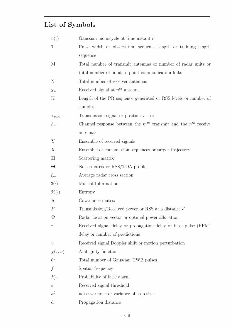
List of Symbols

u(t) Gaussian monocycle at time instant t

T Pulse width or observation sequence length or training length

sequence

M Total number of transmit antennas or number of radar units or

total number of point to point communication links

N Total number of receiver antennas

yn Received signal at nth antenna

K Length of the PR sequence generated or RSS levels or number of

samples

xm,n Transmission signal or position vector

hm,n Channel response between the mth transmit and the nth receive

antennas

Y Ensemble of received signals

X Ensemble of transmission sequences or target trajectory

H Scattering matrix

Θ Noise matrix or RSS/TOA profile

ξav Average radar cross section

I(·) Mutual Information

H(·) Entropy

R Covariance matrix

P Transmission/Received power or RSS at a distance d

Ψ Radar location vector or optimal power allocation

τ Received signal delay or propagation delay or inter-pulse (PPM)

delay or number of predictions

υ Received signal Doppler shift or motion perturbation

χ(τ, υ) Ambiguity function

Q Total number of Gaussian UWB pulses

f Spatial frequency

Pfa Probability of false alarm

ε Received signal threshold

σ2 noise variance or variance of step size

d Propagation distance

viii

α One way path-loss exponent or channel gain

A State transition matrix

B Observation matrix

λ HMM parameter set or SNR or estimated entropy

π Initial probability distribution

amn State transition probability

bmk Observation probability

ZT RSS/TOA observation sequence

QT Target trajectory state sequence

µ Mean vector of received signal

Σ Covariance matrix

o Observation level

ρ Signal to noise ratio

C Capacity of CRR network

X(t) Hidden stochastic process

Y (t) Observation stochastic process

S(t) HMM state of channel occupancy

Pe Probability of error

ix

List of Acronyms

PRF Pulse Repetition Frequency

GCA Ground Control Approach

ATC Air Traffic Control

FM Frequency Modulation

CW Continuous Wave

HF High Frequency

MI Mutual Information

IID Independent and Identically Distributed

MIMO Multiple Input Multiple Output

UWB Ultra-Wideband

PRF Pulse Repetition Frequency

LFM Linear Frequency Modulation

GPS Global Positioning System

NLOS Non Line-of-Sight

pdf Probability Density Function

HMM Hidden Markov Model

OFDM Orthogonal Frequency Division Multiplexing

CRR Cognitive Radar Radio

CRN Cognitive Radar Network

x

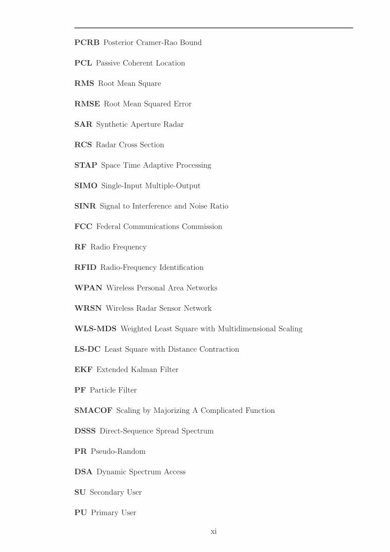
PCRB Posterior Cramer-Rao Bound

PCL Passive Coherent Location

RMS Root Mean Square

RMSE Root Mean Squared Error

SAR Synthetic Aperture Radar

RCS Radar Cross Section

STAP Space Time Adaptive Processing

SIMO Single-Input Multiple-Output

SINR Signal to Interference and Noise Ratio

FCC Federal Communications Commission

RF Radio Frequency

RFID Radio-Frequency Identification

WPAN Wireless Personal Area Networks

WRSN Wireless Radar Sensor Network

WLS-MDS Weighted Least Square with Multidimensional Scaling

LS-DC Least Square with Distance Contraction

EKF Extended Kalman Filter

PF Particle Filter

SMACOF Scaling by Majorizing A Complicated Function

DSSS Direct-Sequence Spread Spectrum

PR Pseudo-Random

DSA Dynamic Spectrum Access

SU Secondary User

PU Primary User

xi

LOS Line-Of-Sight

AWGN Additive White Gaussian Noise

SVD Singular Value Decomposition

AF Ambiguity Function

MSE Mean Squared Error

SCNR Signal-to-Clutter-plus-Noise Ratio

ROC Receiver Operating Characteristics

CFAR Constant False Alarm Rate

RSS Received Signal Strength

TOA Time Of Arrival

MLE Maximum Likelihood Estimation

TDOA Time Difference Of Arrival

AOA Angle Of Arrival

EM expectation-maximization

FIM Fisher Information Matrix

CRLB Cramer-Rao Lower Bound

UMTS Universal Mobile Telecommunications System

SNR Signal to Noise Ratio

PPM Pulse Position Modulation

BER Bit Error Rate

PRI Pulse Repetition Interval

ISI Inter Symbol Interference

CRU Cognitive Radio Users

CBS Cognitive Base Station

xii

CMS Cognitive Mobile Station

CE Cognitive Engine

BWA Baum-Welsh algorithm

ANN Artificial Neural Network

USS Unknown State Sequence

KSS Known State Sequence

xiii

List of Figures

1.1 Differences in the application of information theory to radar system

and communication system design . . . . . . . . . . . . . . . . . . . . 7

1.2 Cognitive Radar Architecture as shown in [33] . . . . . . . . . . . . . 13

1.3 Bat using cognitive echo-location as shown in [33] . . . . . . . . . . . 13

1.4 Cognitive Radar Building blocks . . . . . . . . . . . . . . . . . . . . . 16

3.1 Cognitive MIMO radar architecture. . . . . . . . . . . . . . . . . . . 37

3.2 (a) Transmission waveform at a particular antenna after the two-

step optimization, (b) received signal after matched filtering for the

transmitted signal shown in (a), and (c) target response extraction. . 54

3.3 (a) MSE in target response extraction and (b) probability of target

detection. . . . . . . . . . . . . . . . . . . . . . . . . . . . . . . . . . 55

3.4 AF contours indicating target resolution at (a) iteration 1 and (b)

iteration 20 for a 2 × 2 MIMO radar, which demonstrates a smaller

focal area and an improved signal-to-clutter ratio in (b) as compared

to (a). . . . . . . . . . . . . . . . . . . . . . . . . . . . . . . . . . . . 55

3.5 (a) SAR image, (b) 4× 4 MIMO radar (MI maximization), (c) 4× 4

MIMO radar (MI minimization), and (d) 4×4 MIMO radar two step

MI optimization. (e) ROC for 2 × 2 MIMO radar (f) ROC for 4× 4

MIMO radar. . . . . . . . . . . . . . . . . . . . . . . . . . . . . . . . 57

3.6 (a) Backscatter signal profile for MI minimization at iteration 20,

(b) Backscatter signal profile for MI maximization at iteration 20,

(c) Backscatter signal profile for two-step waveform optimization at

iteration 20, and (d) MSE performance for 4× 4 MIMO configuration. 58

xiv

4.1 10 Voronoi regions formed based on the distribution of 10 radars in

the CRN. The target locations are classified into discrete “states”

corresponding to the Voronoi regions where the target is located. In

the above plot, the sequence of target states is 6 → 8 → 9. . . . . . . 62

4.2 System architecture of the HMM-enabled CRN. . . . . . . . . . . . . 63

4.3 Typical RSS/TOA profiles received at 4 radars. RSS at Radar 1 (the

nearest radar) is quantized into 5 levels. Each level corresponds to a

particular distance from Radar 1 following (4.1). The quantized level

corresponding to the highest RSS is selected. . . . . . . . . . . . . . . 84

4.4 Flowchart for the HMM-based target tracking algorithm. . . . . . . . 85

4.5 Probability of detection for various target tracking algorithms. . . . . 86

4.6 (a) Location estimation errors for various target tracking algorithms,

(b) CRLB on RSS/TOA localization . . . . . . . . . . . . . . . . . . 86

4.7 RMSE performance of the 3 tracking algorithms with respect to vary-

ing values of σνx and σνy . . . . . . . . . . . . . . . . . . . . . . . . . . 87

4.8 An illustrative example for initial and final values (before and after

the training phase) of matrices A and B. . . . . . . . . . . . . . . . . 88

5.1 (a) Coexistence of communication and radar functionalities in a CRR

network, and (b) CRR node architecture. . . . . . . . . . . . . . . . . 109

5.2 (a)column vector of the Walsh-Hadamard code matrix, (b) 16-bit

CRR transmission waveform, (b) orthogonality of CRR waveforms,

and (c) spectrum of the received CRR signal at a reference distance

of 20 m at 4 GHz center frequency. . . . . . . . . . . . . . . . . . . . 110

5.3 (a) Static target and non-target (clutter) scatterers resolved after 10

iterations of MI minimization at a CRR node, and (b) target and

clutter returns after 10 iterations of MI minimization. . . . . . . . . . 111

5.4 (a) Minimization of MI algorithm at different SNRs, (b) probability

of target detection against SCNR for various iterations of the MI

minimization algorithm, and (c) probability of detection for waveform

selection based on MI minimization and static waveform assignment. 112

5.5 (a) BER of different joint communication-radar waveform designs,

and (b) throughput performance against distance from a particular

CRR node. . . . . . . . . . . . . . . . . . . . . . . . . . . . . . . . . 113

xv

5.6 (a) Target range profile for a target velocity = 3.5 m/s for 4 s time

duration after 10 iterations of MI minimization, and (b) target and

clutter returns after 10 iterations of MI minimization. . . . . . . . . . 114

5.7 (a) UWB channel model, (b) average ranging error based on TOA

estimation in the multipath UWB channel, and (c) average ranging

error against PRI in the multipath UWB channel. . . . . . . . . . . . 115

6.1 CRR network architecture. . . . . . . . . . . . . . . . . . . . . . . . . 122

6.2 Proposed training-based HMM system model . . . . . . . . . . . . . . 130

6.3 Proposed HMM state transition . . . . . . . . . . . . . . . . . . . . . 130

6.4 Initial random channel assignment. . . . . . . . . . . . . . . . . . . . 133

6.5 Final location-aware channel assignment. . . . . . . . . . . . . . . . . 134

6.6 CRR network throughput. . . . . . . . . . . . . . . . . . . . . . . . . 134

6.7 Performance of spectrum user detection. . . . . . . . . . . . . . . . . 135

6.8 KSS-HMM prediction accuracy on test data set . . . . . . . . . . . . 136

6.9 Prediction accuracy for a channel . . . . . . . . . . . . . . . . . . . . 137

6.10 Effect of δ value on channel prediction accuracy and spectrum oppor-

tunity usage . . . . . . . . . . . . . . . . . . . . . . . . . . . . . . . . 137

6.11 Comparison of channel selection with prediction and random channel

selection . . . . . . . . . . . . . . . . . . . . . . . . . . . . . . . . . . 139

xvi

List of Tables

4.1 Related Works . . . . . . . . . . . . . . . . . . . . . . . . . . . . . . . 61

4.2 Simulation Setup: Radar Positions . . . . . . . . . . . . . . . . . . . 80

4.3 Execution Times for Various Tracking Algorithms . . . . . . . . . . . 82

6.1 ON/OFF period means for different channels . . . . . . . . . . . . . . 138

6.2 Comparison of KSS-HMM and USS-HMM prediction accuracy . . . . 138

xvii

Chapter 1

Introduction

1.1 Background on Radar Systems

The word radar is an abbreviation for RAdio Detection And Ranging. In general,

radar systems use modulated waveforms and directive antennas to transmit electro-

magnetic energy into a specific volume in space to search for targets [1]. Objects

(targets) within a search volume will reflect portions of this energy (radar returns or

echoes) back to the radar. These echoes are then processed by the radar receiver to

extract target information such as range, velocity, angular position, and other target

identifying characteristics [2]. Radars can be classified as ground based, airborne,

spaceborne, or ship based radar systems [2]. They can also be classified into nu-

merous categories based on the specific radar characteristics, such as the frequency

band, antenna type, and waveforms utilized. Another classification is concerned

with the mission and/or the functionality of the radar. This includes: weather,

acquisition and search, tracking, track-while-scan, fire control, early warning, over

the horizon, terrain following, and terrain avoidance radars [1].

Radars are most often classified by the types of waveforms they use, or by their

operating frequency. Considering the waveforms first, radars can be continuous wave

or pulsed radars [2]. Continuous wave radars are those that continuously emit elec-

tromagnetic energy, and use separate transmit and receive antennas. Unmodulated

continuous wave radars can accurately measure target radial velocity (Doppler shift)

and angular position. Target range information cannot be extracted without uti-

lizing some form of modulation. The primary use of unmodulated continuous wave

radars is in target velocity search and track, and in missile guidance [2]. Pulsed

1

radars use a train of pulsed waveforms (mainly with modulation). In this category,

radar systems can be classified on the basis of the pulse repetition frequency (PRF)

as low PRF, medium PRF, and high PRF radars. Low and medium PRF radars are

primarily used for ranging where target velocity (Doppler shift) is not of interest.

High PRF radars are mainly used to measure target velocity. Continuous wave as

well as pulsed radars can measure both target range and radial velocity by utilizing

different modulation schemes [2]. Radar has been employed on the ground, in the

air, on the sea, and in space. Ground-based radar has been applied chiefly to the

detection, location, and tracking of aircraft or space targets. Shipboard radar is used

as a navigation aid and safety device to locate buoys, shore lines, and other ships, as

well as for observing aircraft. Airborne radar may be used to detect other aircraft,

ships, or land vehicles, or it may be used for mapping of land, storm avoidance,

terrain avoidance, and navigation. In space, radar has assisted in the guidance of

spacecraft and for the remote sensing of the land and sea.

The major user of radar, and contributor of the cost of almost all of its devel-

opment, have been the military, although there have been increasingly important

civil applications, chiefly for marine and air navigation [2]. As indicated in [2], the

major areas of radar application, in no particular order of importance, are briefly

described below.

• Air Traffic Control (ATC): Radars are employed throughout the world for

the purpose of safely controlling air traffic en-route and in the vicinity of

airports. Aircraft and ground vehicular traffic at large airports are monitored

by means of high-resolution radar. Radar has been used with GCA (ground-

control approach) systems to guide aircraft to a safe landing in bad weather.

In addition, the microwave landing system and the widely used ATC radar-

beacon system are based in large part on radar technology.

• Aircraft Navigation: The weather-avoidance radar used on aircraft to out-

line regions of precipitation to the pilot is a classical form of radar. Radar is

also used for terrain avoidance and terrain following. Although they may not

always be thought of as radars, the radio altimeter (either frequency modu-

lation (FM)/continuous wave (CW) or pulse) and the Doppler navigator are

also radars. Sometimes ground-mapping radars of moderately high resolution

are used for aircraft navigation purposes.

2

• Ship Safety: Radar is used for enhancing the safety of ship travel by warning

of potential collision with other ships, and for detecting navigation buoys,

especially in poor visibility. In terms of numbers, this is one of the largest

applications of radar, but in terms of physical size and cost it is one of the

smallest. It has also proven to be one of the most reliable radar systems.

Automatic detection and tracking equipments (also called plot extractors) are

commercially available for use with such radars for the purpose of collision

avoidance. Shore-based radar of moderately high resolution is also used for

the surveillance of harbors as an aid to navigation.

• Remote Sensing: All radars are remote sensors; however, as this term is used

it implies the sensing of geophysical objects, or the “environment.” For some

time, radar has been used as a remote sensor of the weather. It was also used

in the past to probe the moon and the planets (radar astronomy). The iono-

spheric sounder, an important adjunct for high frequency (HF) (short wave)

communications, is a radar. Remote sensing with radar is also concerned

with Earth resources, which includes the measurement and mapping of sea

conditions, water resources, ice cover, agriculture, forestry conditions, geolog-

ical formations, and environmental pollution. The platforms for such radars

include satellites as well as aircraft.

• Law Enforcement: In addition to the wide use of radar to measure the speed

of automobile traffic by highway police, radar has also been employed as a

means for the detection of intruders.

• Military: Many of the civilian applications of radar are also employed by

the military. The traditional role of radar for military application has been

for surveillance, navigation, and for the control and guidance of weapons. It

represents, by far, the largest use of radar.

1.2 Recent Advances and Research Scope

As mentioned in the abstract, this thesis aims at developing cognitive mechanisms

for designing modern radar systems. The purpose of this section is to introduce

these modern technological advances and indicate the scope for improvement by

3

utilizing a cognitive architecture. Specifically, this thesis focuses on three domains

of radar research,

1. Radar waveform design and optimization strategies for target discrimination

in presence of clutter and non-stationary radar environments.

2. Target detection, tracking and target parameters extraction in indoor and

outdoor radar applications.

3. Radars equipped with added functionalities like the joint communication-

radars.

1.2.1 Radar Waveform Design and Optimization Strategies

for Target Discrimination

Adaptive waveform design for radar applications has been a well investigated subject

in the past. Some of the pioneering works like [3], have applied information-theoretic

measures for the design of radar waveforms in order to facilitate improved target

detection and classification. The basic difference between the application of informa-

tion theory in communication and radar systems design has been shown in Fig. 1.1.

In communication systems design, the source of uncertainty of information lies at

the transmitter, since the receiver has no knowledge of the transmitted signal. Here

we intend to make the received signal statistically more dependant on the trans-

mitted signal in order to reduce the bit error rate. Hence the basic objective is to

maximize the mutual information between the received signal and the transmitted

signal in order to improve the overall information capacity of the communication

system. However as seen from Fig. 1.1, the source of uncertainty or information in

the radar system lies at the target. In this case, the receiver has an exact knowledge

of the transmitted signal. Thus the distortion brought about by the target upon the

transmitted signal is a matter of interest to us. In radar systems we want to ensure

that the transmission waveforms would be designed with the sole objective of mak-

ing the received signal more statistically dependant upon the target signature, and

we intend to suppress the non-target contributions from noise and clutter. Thus,

in this case we intend to maximize the mutual information between the received

signal and the estimated target impulse response given the transmission signal. In

this thesis we explore such a waveform optimization approach which allows us to

4

design optimum transmission waveforms which would “match” the target based on

the information-theoretic measures.

In recent years, the research on the development of knowledge-aided waveform

design has received great impetus. Some of the noteworthy works in this area

include [4–8]. In these works the radar transmission parameters are modified in

order to improve the target parameters estimation in a dynamic radar environment.

Based on the prior knowledge about targets and environments, transmit signals can

be adaptively optimized to improve system performance and efficiency. Inspired

by this concept, many attempts have been focusing on target recognition using

waveform-adaptation. In [9], Goodman proposed the integration of waveform de-

sign techniques with a sequential-hypothesis testing framework [10] that controls

when hard decisions may be made with adequate confidence [6]. He also compared

two different waveform design techniques for use with active sensors operating in a

target recognition application. One is based on a maximization of the mutual infor-

mation (MI) between a random target ensemble and the echo signal, while the other

is based on maximizing the weighted average Euclidean distance or Mahalanobis

distance (in additive colored noise) between the ideal echoes from different target

hypotheses [8, 10], where known impulse responses are used to model the target

scattering behaviors.

Multiple-input multiple-output (MIMO) radar has attracted more and more at-

tention of researchers in recent times. The concept of MIMO has appeared in the

field of communication system since the 1990s. However, it has not appeared in sen-

sor and radar systems until recently [11]. Unlike the standard phased array radar

transmitting a single waveform at a time, MIMO radar transmits multiple orthogo-

nal waveforms by multiple antennas simultaneously. These waveforms are extracted

by a bank of matched filters in the receiver. All the matched filter output are then

combined to obtain the desired information [12]. Recent theoretical research has

shown some advantages to operate a radar in MIMO mode, e.g., improved target

detecting performance, better target model parameter estimation and target im-

age creation [13]. However, from a system engineering viewpoint, there are serious

tradeoffs of MIMO versus phased array radars relative to cost, system complexity

and risk and it is not clear what advantages MIMO radar offers [13]. MIMO radars

can be broadly classified into 2 categories, distributed and collocated MIMO archi-

tectures. In the distributed MIMO radar scene the MIMO transmitter and receiver

5

elements are spatially separated by a significant distance. This allows the different

transceiver units to view the target from distinct aspect angles and thus the MIMO

receiver can exploit the spatial diversity of the MIMO channel. In this thesis, we

evaluate a distributed MIMO architecture in Chapter 3.

Research Scope

Most of the research pertaining to statistical characterization of radar scene, treats

clutter as a wide sense stationary random process. Nevertheless, focusing on the

scattering phenomena that give rise to the received signal, we observe that the re-

ceived clutter depends on the radar scene in a certain temporal range. Thus, the

clutter process cannot be stationary, particularly over long time intervals. Mitiga-

tion of Doppler spread clutter can be achieved by estimating the covariance matrix

of slow-time data across the coherent processing interval. Typically, this covariance

matrix is estimated by averaging snapshots of the slow-time clutter time series at

neighboring range bins [14]. However in complex propagation conditions, the clutter

return is often “non-stationary” in range which seriously limits the availability

of independent, identically distributed (IID) signal-free training data [15].

For such radar scenarios, which are heavily cluttered and non-stationary, MIMO

radars offer attractive solutions to enhance target detection and discrimination.

MIMO radar empowered with a cognitive architecture can facilitate efficient target

discrimination by exploiting the spatial diversity, waveform diversity and by adopt-

ing a cognitive approach through continual interactions with the radar environment.

Consequently, such a radar would be able to adjust its operational parameters like

the transmit power, waveform shape and frequency “on the fly” and in a completely

autonomous manner. In this thesis, Chapter 3 extends the relevant works on infor-

mation theoretic waveform design to waveform optimization in MIMO radars. In

this Chapter, the concept of MI is used to design and select the MIMO waveforms.

The objective of this algorithm is to extract the target impulse response from the

radar scene which is heavily cluttered and non-stationary.

6

Figure 1.1: Differences in the application of information theory to radar system andcommunication system design

1.2.2 Target Detection, Tracking and Parameter Extraction

in Indoor Radar Applications

Over past several decades there has been an extensive research on designing efficient

radar illumination strategies for target detection and tracking applications. Wire-

less radar sensor network is emerging as an enabling technology for applications such

as border surveillance, intrusion monitoring for unauthorized movement of targets

around critical facilities. Surveillance applications, i.e., real-time detection, tracking

and classification of intrusion, require mission critical networking capabilities in wire-

less sensor networks [16]. Generally, low power ultra-wideband (UWB) radar sensors

are used in detection, tracking and localization of an intruder in sensor field [17,18].

The proliferation of wireless localization technologies provides a promising future for

serving human beings in indoor scenarios. Their applications include real-time track-

ing, activity recognition, health care, navigation, emergence detection, and target-

of-interest monitoring, among others. Additionally, indoor localization technologies

address the inefficiency of Global Positioning System (GPS) inside buildings [16].

However, due to the complex of indoor environments, the development of an indoor

localization technique is always accompanied with a set of challenges, e.g. non line of

sight (NLOS), multipath effect, and noise interference [19]. These challenges result

7

mainly from the influence of obstacles (e.g. walls, equipments, and human beings)

on the propagation of electromagnetic waves. For instance, the mobility of people

incurs changes in physical conditions of the environment, which might significantly

affect the behavior of wireless radio propagation. Although these negative effects

cannot be eliminated completely, in recent years researches are constantly going on

to improve the performance of indoor (human/object) tracking.

The use of location and tracking information is an excellent tool to improve pro-

ductivity and to optimize the resources management in a wide range of sectors [20]:

industry, medicine, home-automation or military. An additional potentiality of the

tracking problem that has not been explored enough is the mobility of the moving

targets, especially for the complex surroundings [21]. The Kalman filter can get

the optimal solution to the tracking problem in the assumption of linear Gaussian

environment. However, in many situations of interest, the assumptions made above

do not hold. The extended Kalman filter [22] utilizes the first term in a Taylor

expansion of the nonlinear function, but the required probability density function

(pdf) is still approximated by a Gaussian, which may be a gross distortion of the

true underlying structure and may lead to filter divergence.

Research Scope

Design of indoor localization and tracking radar systems is a challenging research

field. There is a need for employing a radar architecture which can adapt au-

tonomously and effectively to the dynamic radar environment. The indoor wire-

less environment is rich in multipath and clutter sources, which can prove to be

detrimental to target detection and tracking. These problems can be alleviated by

adopting a cognitive architecture in the design of the indoor radar systems, which

would constantly learn from the extracted target parameters information for the

radar scene. In this way, intelligent illumination strategies could be devised which

ensure effective target illumination in the indoor radar environment. This problem

is dealt with in more detail in Chapter 4 of this thesis. In this Chapter, a cognitive

illumination strategy for an indoor cognitive radar network is devised which learns

from the target trajectory by utilizing a hidden Markov model (HMM) thus improv-

ing the target detection and tracking performance. By adopting this framework, the

tracking algorithm is more robust to rapid target movements and alleviates some of

the problems like the Gaussian approximations which are made in the contemporary

tracking algorithms.

8

1.2.3 Joint Communication-Radar System Design

Wireless communications and radar have always been independent research enti-

ties in the past. Wireless communications focus upon achieving the best possible

information capacity across a noisy wireless channel under power and complexity

constraints. On the other hand, radar systems attempt to achieve better target res-

olution and parameter estimation in the presence of surrounding clutter and noise.

In recent years, the research in integrating the communication and radar system

designs under a common platform has gained significant momentum [23–29]. Such

a joint radar and communication system would constitute a unique cost-efficient so-

lution for future intelligent surveillance applications, for which both environmental

sensing and establishment of ad hoc communication links is essential. This type

of systems can be used in mission-critical and military operations to address the

surveillance and communication issues simultaneously [24]. It is thus envisaged that

future personal communication devices will have comprehensive radar-like functions

such as spectrum sensing and localization, in addition to multi-mode and multi-band

communication capability. Recent works such as [24] and [25] in particular focus

upon the development of devices that have multiple radio functions and combine

communication and radar in a small portable form with ultra low power consump-

tion.

Communication information can be embedded in the radar system through wave-

form diversity [30,31]. Meanwhile, in the radar network, the communication message

for instance the reports on the detected targets can be embedded into the orthogo-

nal frequency division multiplexing (OFDM) radar waveform [32]. A unique covert

opportunistic spectrum access solution to enable the coexistence of OFDM based

data communication with UWB noise radar is presented in [33]. A multi-functional

waveform has been designed, by embedding an OFDM signal within a spectrally

notched UWB random noise waveform [33].

Research Scope

There is a significant research potential in the design of joint communication-radar

systems. An interesting extension to this research problem is developing cognitive

waveform design solution which would adapt to the dynamic radar scene while still

maintaining the communication link between radar units. Another aspect of this

research is the fusion of the cognitive radar and cognitive radio paradigms for wire-

9

less network applications. The research on cognitive radar and cognitive radio is

beginning to gain momentum in recent years. Both of these models strive to im-

part intelligence to traditional wireless systems which utilize a static framework for

resource management and hence are not able to cope up with the ever increasing

demands of wireless devices being deployed.

In this thesis, Chapter 5 investigates such a joint communication-radar network

by employing cognitive radar principles. In this Chapter, a novel system archi-

tecture and waveform design method has been illustrated for cognitive radar radio

(CRR) networks. Chapter 6 further extends this idea and utilizes the superior tar-

get parameter extraction capability of cognitive radars to allocate crucial resources

like power, spectrum over the wireless network. This Chapter also illustrates the

fusion of cognitive radar and cognitive radio paradigms for exploring opportunistic

spectrum access methods for improving the channel sensing abilities of the wireless

devices in a network.

1.3 Motivation for Cognitive Radar System De-

sign

According to the Oxford English Dictionary, cognition is “knowing, perceiving, or

conceiving as an act”. Cognitive radar network (CRN) is an innovative paradigm for

optimizing radar surveillance within non-stationary environments, where the radar

scene can be highly time-variant [34–37]. As mentioned in [35], the three ingredients

are basic to the constitution of a cognitive radar:

1. Intelligent signal processing, which builds on learning through interactions of

the radar with the surrounding environment;

2. Feedback from the receiver to the transmitter, which is a facilitator of intelli-

gence;

3. Preservation of the information content of radar returns, which is realized by

the Bayesian approach to target detection through tracking.

This cognitive approach to radar design is possible because of the three distinct

capabilities of modern radars [35]:

1. The inherent ability of radar to sense its environment on a continuous basis

10

2. The ability of phased-array antennas to electronically scan the environment in

a fast manner

3. The ever-increasing power of computers to digitally process signals

From the moment a surveillance radar system is switched on, the system becomes

electromagnetically linked to its surrounding environment in the sense that the en-

vironment has a strong and continuous influence on the radar returns (i.e., echoes).

In so doing, the radar builds up its knowledge of the environment from one scan to

the next and makes decisions of interest on possible targets at unknown locations in

the environment; the locations are not known before the radar is switched on, but

they become determined by the radar receiver once the targets under surveillance

are declared. From signal processing and control theory perspective, we know that

it is not necessary for the radar to keep the entire record of past data [35]. Rather,

by adopting a state-space model of the environment and recursively updating the

state vector representing an estimate of certain parameters pertaining to the envi-

ronment, the need for storing the entire history of radar data on the environment

is eliminated [34, 35]. The requirement to update estimation of the environmental

state is necessitated by the fact that the radar environment is non-stationary.

Recursive updating of a state is synonymous with adaptivity, which is the nat-

ural method for dealing with non-stationarity. In current designs of radar systems,

however, adaptivity is usually confined to the receiver [36]. For a radar to be cogni-

tive, adaptivity has to be extended to the transmitter too. Moreover, the radar has

to learn from experience on how to deal with different targets, large and small, and

at widely varying ranges, all in an effective and robust manner.

This way of thinking leads us to the block diagram of Figure 1.2, which depicts

the picture of a cognitive cycle performed by a cognitive radar system. The cycle

begins with the transmitter illuminating the environment. The radar returns pro-

duced by the environment are fed into two functional blocks: radar-scene analyzer

and Bayesian target-tracker. The tracker makes decisions on the possible presence

of targets on a continuing time basis, in light of information on the environment

provided to it by the radar-scene analyzer. The transmitter, in turn, illuminates

the environment in light of the decisions made on possible targets, which are fed

back to it by the receiver. The cycle is then repeated over and over again. Note

also that although the process of target detection is not explicitly shown in the cog-

11

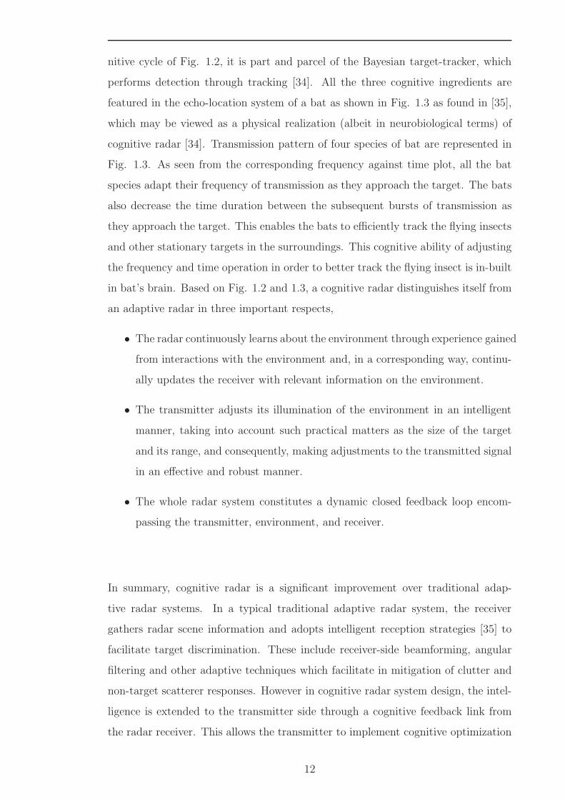
nitive cycle of Fig. 1.2, it is part and parcel of the Bayesian target-tracker, which

performs detection through tracking [34]. All the three cognitive ingredients are

featured in the echo-location system of a bat as shown in Fig. 1.3 as found in [35],

which may be viewed as a physical realization (albeit in neurobiological terms) of

cognitive radar [34]. Transmission pattern of four species of bat are represented in

Fig. 1.3. As seen from the corresponding frequency against time plot, all the bat

species adapt their frequency of transmission as they approach the target. The bats

also decrease the time duration between the subsequent bursts of transmission as

they approach the target. This enables the bats to efficiently track the flying insects

and other stationary targets in the surroundings. This cognitive ability of adjusting

the frequency and time operation in order to better track the flying insect is in-built

in bat’s brain. Based on Fig. 1.2 and 1.3, a cognitive radar distinguishes itself from

an adaptive radar in three important respects,

• The radar continuously learns about the environment through experience gained

from interactions with the environment and, in a corresponding way, continu-

ally updates the receiver with relevant information on the environment.

• The transmitter adjusts its illumination of the environment in an intelligent

manner, taking into account such practical matters as the size of the target

and its range, and consequently, making adjustments to the transmitted signal

in an effective and robust manner.

• The whole radar system constitutes a dynamic closed feedback loop encom-

passing the transmitter, environment, and receiver.

In summary, cognitive radar is a significant improvement over traditional adap-

tive radar systems. In a typical traditional adaptive radar system, the receiver

gathers radar scene information and adopts intelligent reception strategies [35] to

facilitate target discrimination. These include receiver-side beamforming, angular

filtering and other adaptive techniques which facilitate in mitigation of clutter and

non-target scatterer responses. However in cognitive radar system design, the intel-

ligence is extended to the transmitter side through a cognitive feedback link from

the radar receiver. This allows the transmitter to implement cognitive optimization

12

Figure 1.2: Cognitive Radar Architecture as shown in [33]

Figure 1.3: Bat using cognitive echo-location as shown in [33]

strategies to enhance target parameters extraction. Cognitive radar systems show

improvement in target discrimination by adopting a multiple iterative approach to

adapt and learn about the radar scene in real time.

A CRN [38] incorporates several radars working together to achieve the task of

enhanced remote sensing capability. The network can operate in two modes, dis-

tributed cognition and central cognition. In a distributed cognitive network, each

radar is capable of cognitive processing, whereas in a central cognitive network, a

single radar acts as the brain of the entire network. With several radars operating

in parallel, the system performance is considerably improved over a single radar.

Several problems have been addressed in the past under the closed-loop cognitive

13

framework. In this thesis, both of these central and distributed cognitive archi-

tectures have been explored. Specifically, in Chapters 3 and 4, a central cognitive

architecture is adopted, in the rest of the Chapters a more distributed cognitive

approach is investigated.

The cognitive framework is illustrated in Fig. 1.4. As shown in Fig. 1.4, the

cognitive framework consists of a closed loop involving the adaptive control over

operational parameters of the radar system, the radar environment, the perception

of the environment gained through constant interactions with it and the feedback

channel that allows the adaptive control. Also the fundamental building blocks for

the cognitive radar system which differentiate it from the traditional radar systems

are shown in Fig. 1.4. The authors of [9] integrate waveform design, based on the

maximization of MI, with sequential hypothesis testing. In [39], the authors use

a cognitive radar for single-target tracking and propose a waveform optimization

based on the minimization of the posterior Cramer-Rao bound (PCRB). In [40], the

authors employ dynamic programming to select optimal waveforms from a prescribed

library using PCRB as an optimization criterion. In [41], the authors use a CRN for

extended target recognition, and in [42], the authors propose an adaptive waveform

design for a cognitive radar for target recognition. Finally, in [43], the authors

describe time resource allocation techniques for a cognitive radar system.

In [44] the author proposes a cognitive version of passive coherent location (PCL)

which has much in common with the broad cognitive radar concept, but adapts only

to the waveforms it senses in the environment, and exploits those that are most

useful to it for target detection. In addition, it would model the terrain to improve

coverage and provide countermeasures against direct signal saturation. By its name,

PCL does not transmit, but relies on emissions from other radiating systems, such

as broadcast services, other radars, cellular radio, WiFi, and so on. It is clear that

such a cognitive system, consisting of multiple, cooperating receivers, can achieve

excellent performance in the presence of deliberate jamming, difficult terrain, and

attempts at target stealth.

When the targets are moving in a dense urban environment, this problem be-

comes much more challenging [45]. The propagation path in such an environment

consists of multiple scatterers, which can be in relative motion with respect to the

sensors. This introduces both delay and Doppler shift in the received signals. To

exploit this inherent delay-Doppler diversity and to obtain better performance, ac-

14

curate prior information about the multipath channel state is required. When no

prior information is available, the channel state has to be estimated along with the

target state. When multiple sensors are employed, the channel state between each

pair of sensors has to be estimated. Hence, the problem of tracking multiple tar-

gets in complex scenarios, such as an urban environment, poses a computational

challenge due to the high-dimensionality of the state space.

For an active sensor network, such as a radar network, it is also important to con-

sider the constraints on the signal power to be transmitted, and the sensor locations

while formulating the optimization problem. Few works in the past have addressed

the problem of sensor scheduling for active sensor networks like a distributed MIMO

radar network. In [46], the authors propose a subset selection algorithm for the task

of estimating the position of a single stationary target. They assume that there is no

multipath and the signals transmitted from each radar are orthogonal to each other.

In [47], the authors consider tracking multiple targets. They perform an iterative

local search to minimize the PCRB and find a subset of antennas to be employed

at each time.

In [48], the authors investigate a CRN system for the joint estimation of the

target state comprising the positions and velocities of multiple targets, and the

channel state comprising the propagation conditions of an urban transmission chan-

nel. They develop a measurement model for the received signal by considering a

finite-dimensional representation of the time-varying system function which char-

acterizes the urban transmission channel. The authors employ sequential Bayesian

filtering at the receiver to estimate the target and the channel state. They propose

a hybrid Bayesian filter that operates by partitioning the state space into smaller

subspaces and thereby reducing the complexity involved with high-dimensional state

space. The feedback loop that embodies the radar environment and the receiver en-

ables the transmitter to employ approximate greedy programming to find a suitable

subset of antennas to be employed in each tracking interval, as well as the power

transmitted by these antennas. The PCRB on the target and channel state esti-

mation is used as an optimization criterion for designing the antenna selection and

power allocation algorithms.

15

Figure 1.4: Cognitive Radar Building blocks

1.4 Major Contributions and Thesis Outline

In this thesis, we develop and analyze cognitive radar architectures to improve tar-

get parameter extraction from a radar scene. The radar scene considered is dynamic

with mobile target and non-target scatterers. Specifically this work focuses on the

intelligent illumination techniques for the radar scene based on cognition. As dis-

cussed previously, this thesis aims at developing cognitive mechanisms which would

gain from adaptive waveform design methods, continual learning based on constant

interactions with the radar environment and developing feedback mechanisms which

would make the radar transmitter more “intelligent” and aware about the dynamic

target scene.

In particular, we try to incorporate the above mentioned recent advances in

radar systems design within the cognitive radar framework. We develop cognitive

architectures for MIMO radar, UWB radar and joint communication-radar waveform

design applications. Specifically, we incorporate the cognitive framework for MIMO

radar through a novel waveform optimization algorithm, we develop a cognitive

strategy for target detection and tracking for UWB radars and finally we investigate

the radar systems with added functionality by developing joint communication-radar

systems. Chapter-wise major contributions of this thesis are as follows:

• In Chapter 2, a detailed literature survey on the research ideas mentioned in

Section 1.2 is presented. Specifically recent advances in MIMO, UWB and

joint communication-radar systems are discussed in detail in this Chapter.

• In Chapter 3, a cognitive MIMO radar waveform design method is developed

and analyzed. In this approach the target parameter estimates formed by

the radar receiver through successive interactions with the radar environment

are used in order to design MIMO radar waveforms. This novel two-step ap-

16

proach employs information theoretic concepts in order to design the MIMO

waveforms. As demonstrated by this work the cognitive MIMO waveform de-

sign approach improves the target parameter extraction capability. Simulation

results also demonstrate that the cognition improves target detection proba-

bility, target impulse response or target signature extraction capability and

delay-Doppler resolution.

• In Chapter 4, a CRN is developed for facilitating intelligent illumination of the

radar scene. This approach employs spatial discretization of the radar scene

and develops a HMM enabled approach to learn about the target trajectory.

This work considers a distributed radar network which has been deployed to

track the trajectory of a target. The radar system learns from the target

trajectory and updates its understanding about the radar scene with every

subsequent scan. This updated understanding of the radar scene facilitates

the intelligent illumination in the succeeding time instant. As demonstrated

by the simulation results, the performance gain in terms of probability of

target detection, root mean squared (RMS) error on location and tracking

performance is compared with the benchmark methods for tracking.

• In Chapter 5, a joint communication-radar waveform design is developed based

on cognition. In this chapter a novel approach for encapsulating communica-

tion and radar functionalities in a single waveform design for CRR networks

is proposed. This approach aims at extracting the target parameters from

the radar scene, as well as facilitating high data rate communications between

CRR nodes by adopting a single waveform optimization solution. Each CRR

node encapsulates its communication data into the radar signal such that the

radio and radar information is always separable and can be shared over the en-

tire network. Such CRR networks are aimed at addressing the communication

and radar detection problems in mission-critical and military applications,

where there is a need of integrating the knowledge about the target scene

gained from distinct radar entities functioning in tandem with each other.

• In Chapter 6, a novel approach to spectrum and power allocation is proposed

for cognitive radio networks by integrating cognitive radio and cognitive radar

network paradigms to achieve intelligent utilization of spectral resources in a

17

wireless network. This approach exploits the intelligent location information

offered by cognitive radars combined with user detection capability of cognitive

radios to aid spectrum and power allocation to minimize interference between

wireless devices. Such a system requires sharing of channel perception between

the radio and radar devices involved, to aid better spectral resource utilization.

The second aspect of this research is investigating the inclusion of cognitive

mechanism in predicting the spectral holes over the network by adopting a

HMM learning approach. To realize opportunistic spectrum access, cognitive

spectrum sensing is applied to detect the presence of spectrum holes. Simula-

tion results indicate improvement in throughput and reduction in interference

between neighboring wireless devices.

• Finally, Chapter 7 provides concluding remarks and associated future works

for this research.

Throughout this work, det(·) denotes the determinant of a matrix, (·)H denotes

the Hermitian transpose, tr(·) denotes the trace, and E· denotes the expectation

operator.

1.5 Publications Arising From This Research

1. Y. Nijsure, Y. Chen, C. Litchfield and P. B. Rapajic, “Hidden Markov model

for target tracking with UWB radar systems”, in Proc. IEEE 20th Interna-

tional Symposium on Personal, Indoor and Mobile Radio Communications,

pp. 2065-2069, 13-16 Sept. 2009.

2. Y. Nijsure, Y. Chen, P. Rapajic, C. Yuen, Y. H. Chew, and T. F. Qin,

“Information-theoretic algorithm for waveform optimization within ultra wide-

band cognitive radar network”, in Proc. IEEE International Conference on

Ultra-Wideband (ICUWB), vol. 2, Sept. 2010, pp. 1-4.

3. Y. Nijsure, Y. Chen, C. Yuen, Y. H. Chew, “Location-aware spectrum and

power allocation in joint cognitive communication-radar networks”, in Proc.

Cognitive Radio Oriented Wireless Networks and Communications (CROWN-

COM), pp.171-175, 1-3 June 2011.

18

4. H. Ahmadi, Y. H. Chew, P. K. Tang and Y. Nijsure,“Predictive opportunistic

spectrum access using learning based hidden Markov models”, in Proc. IEEE

22nd International Symposium on Personal Indoor and Mobile Radio Commu-

nications (PIMRC), pp.401-405, 11-14 Sept. 2011.

5. Y. Nijsure, Y. Chen, Y. Chau, Y. H. Chew, Z. Ding and S. Boussakta,“Adaptive

Distributed MIMO Radar Waveform Optimization Based on Mutual Infor-

mation”, IEEE Transactions on Aerospace and Electronic Systems (Journal

accepted for publication in September 2012).

6. Y. Nijsure, Y. Chen, P. Rapajic, C. Yuen and Y.H. Chew,“Mobile target track-

ing using hidden-Markov-model-enabled Cognitive Radar Network”, IEEE

Transactions on Aerospace and Electronic systems (Journal under 2nd stage

review).

7. Y. Nijsure, Y. Chen, Y. Chau, Y. H. Chew, Z. Ding and S. Boussakta,“Novel

system architecture and waveform design for cognitive radar radio Networks”,

IEEE Transactions on Vehicular Technology(Journal accepted for publication

in May 2012).

19

Chapter 2

Literature Survey

2.1 Introduction

As mentioned in Chapter 1, this thesis provides a cognitive approach to design the

modern radar systems. In Section 1.2, the link between the existing research ideas

and the contribution of this thesis was presented. In this Chapter, a detailed lit-

erature survey on these research ideas is provided. Specifically, recent advances in

MIMO, UWB and joint communication-radar systems are discussed in detail. We

incorporate the cognitive framework for MIMO radar through a novel waveform

optimization algorithm, we develop a cognitive strategy for target detection and

tracking for UWB radars and finally we investigate the radar systems with added

functionality by developing joint communication-radar systems. We further inves-

tigate the fusion of the cognitive radar and cognitive radio paradigms for enhanced

spectrum and power resource allocation in wireless networks.

2.2 MIMO Radar System

MIMO radar is an emerging technology that is attracting the attention of radar

researchers. Unlike a standard phased array radar, which transmits scaled versions

of a single waveform, a MIMO radar system can transmit via its antennas multi-

ple probing signals that may be chosen quite freely. The notion of MIMO radar

is simply that there are multiple radiating and receiving sites [49]. The collected

information is then processed together. In some sense, MIMO radars are a gener-

alization of multi-static radar [50, 51]. The underlying concepts have most likely

20

been discovered independently numerous times. By the most general definition,

many traditional systems can be considered as special cases of MIMO radars. As

an example, synthetic aperture radar (SAR) can be considered as a form of MIMO

radar. Although SAR traditionally employs a single transmit antenna and a single

receive antenna, the positions of these two antennas are translated and images are

formed by processing all the information jointly. The significant difference between

this radar and a “typical” MIMO radar, which takes full advantage of the degrees of

freedom, is that SAR does not have access to channel measurements for all transmit-

receive position pairs. Equivalently, one may say that only the diagonal elements

of the channel matrix are measured. Similarly, a fully polarimetric radar, that is, a

radar that measures both receive polarizations for each transmit polarization, is an

example of MIMO radar [50]. Clearly, it is a MIMO radar with a relatively small

dimensionality. In addition, some spatial interpretations of MIMO radar have to be

considered in a different context for polarimetric radars.

The transmit antennas radiate signals, which may or may not be correlated, and

the receive antennas attempt to disentangle these signals. In much of the current

literature, it is assumed that the waveforms coming from each transmit antenna are

orthogonal, but this is not a requirement for MIMO radar. However, orthogonality

can facilitate the processing. Two simple approaches to obtain orthogonality are

to use time division or frequency division multiplexing. However, both approaches

can suffer from potential performance degradation (assuming coherent operation)

because of the loss of coherence of the target response. The scattering response of

the target or background is commonly time-varying or frequency-selective, limiting

the ability to coherently combine the information from the antenna pairs. In some

applications, it is desirable to introduce correlation between the transmitted signals.

For some tracking problems, optimal asymptotic angle estimation performance is

given by employing strongly correlated signals [49].

There is a continuum of MIMO radar system concepts; however, there are two

basic regimes of operation considered in the current literature. In the first regime,

the transmit array elements (and receive array elements) are broadly spaced, pro-

viding independent scattering responses for each antenna pair, sometimes referred

to as statistical MIMO radar. In the second regime, the transmit array elements

(and receive array elements) are closely spaced so that the target is in the far field

of the transmit or receive array, sometimes referred to as coherent MIMO radar.

21

Here it is assumed that the targets scattering response is the same for each antenna

pair, up to some small delay. While the answer to the question,“how large must

the angular separation be to get independent scattering responses?” is dependent

on the details of the target, a sense of scale is provided by thinking of the target

as an array of scatterers with phase responses optimized to focus energy toward

one of the antennas. If an array of appropriately phased scatterers of the physical

size of the target can resolve individual locations of the antennas, then independent

scattering responses would theoretically be possible [49]. The waveform diversity

enables superior capabilities compared with a standard phased array radar.

In [11, 49, 52, 53], the diversity offered by widely separated transmit/receive an-

tenna elements was exploited. Many other papers, including, for instance, [54], have

considered the merits of a MIMO radar system with collocated antennas. The advan-

tages of a MIMO radar system with both collocated and widely separated antenna

elements are investigated in [55]. For collocated transmit and receive antennas, the

MIMO radar paradigm has been shown to offer higher resolution [50,56], higher sen-

sitivity to detecting slowly moving targets [57], better parameter identifiability [58],

and direct applicability of adaptive array techniques [58, 59]. On the other hand,

MIMO radars employing widely separated antennas have an advantage of viewing

the target from several distinct aspect angles. The radar cross section (RCS) of the

target varies with the aspect angle and thus widely separated MIMO radar systems

can exploit spatial diversity more effectively [49]. Waveform optimization has also

been shown to be a unique capability of a distributed MIMO radar system. For

example, it has been used to achieve flexible transmit beam pattern designs [60] as

well as for MIMO radar imaging and parameter estimation [54].

In the MIMO radar receiver, a matched filter bank is used to extract the or-

thogonal waveform components. There are two different approaches for using the

non-coherent waveforms:

1. Increased spatial diversity can be obtained [52,53]. In this scenario, the trans-

mitting antenna elements are far enough from each other relative to the dis-

tance from the target. The target RCSs are independent random variables for

different transmitting paths. When the orthogonal components are sent from

different antennas, each orthogonal waveform will carry independent informa-

tion about the target. This spatial diversity can be utilized to perform better

22

detection [52, 53].

2. A better spatial resolution for clutter can be obtained. In this scenario, the

distances between transmitting antennas are small enough compared to the

distance between the target and the radar station such that the target RCS

is identical for all transmitting paths. The phase differences caused by differ-

ent transmitting antennas along with the phase differences caused by different

receiving antennas can form a new virtual array steering vector. With judi-

ciously designed antenna positions, one can create a very long array steering

vector with a small number of antennas. Thus the spatial resolution for clutter

can be dramatically increased at a small cost.

The adaptive techniques for processing the data from airborne antenna arrays

are called space time adaptive processing (STAP) techniques. The basic theory of

STAP for the traditional single-input multiple-output (SIMO) radar has been well

developed [61]. Many algorithms have been proposed for improving the complexity

and convergence of the STAP in the SIMO radar. With a slight modification, these

methods can also be applied to the MIMO radar case. The MIMO radar STAP for

multipath clutter mitigation can be found in [62]. However, in the MIMO radar,

STAP becomes even more challenging because of the extra dimension created by

the orthogonal waveforms. On one hand, the extra dimension increases the rank of

the jammer and clutter subspace, especially the jammer subspace. This makes the

STAP more complex. On the other hand, the extra degrees of freedom created by

the MIMO radar allow us to filter out more clutter subspace with little effect on

signal-to-interference-and-noise ratio (SINR).

2.3 UWB Radars

UWB radio is a fast emerging technology with uniquely attractive features inviting

major advances in wireless communications, networking, radar, imaging, and posi-

tioning systems. By its rule-making proposal in 2002, the Federal Communications

Commission (FCC) in the United States essentially unleashed huge new bandwidth

(3.6 − 10.1 GHz) at the noise floor, where UWB radios overlaying coexistent ra-

dio frequency (RF) systems can operate using low-power ultra-short information

bearing pulses. With similar regulatory processes currently under way in many

23

countries worldwide, industry, government agencies, and academic institutions re-

spond to this FCC ruling with rapidly growing research efforts targeting a host of

exciting UWB applications. These include short-range very-high-speed broadband

access to the Internet, covert communication links, localization at centimeter-level

accuracy, high-resolution ground-penetrating radar, through-wall imaging, precision

navigation and asset tracking, just to name a few. UWB characterizes transmission

systems with instantaneous spectral occupancy in excess of 500 MHz or a fractional

bandwidth of more than 20%. Such systems rely on ultra-short (nanosecond scale)

waveforms that can be free of sine-wave carriers and do not require intermediate fre-

quency processing because they can operate at baseband. As information-bearing

pulses with ultra-short duration have UWB spectral occupancy, UWB signals come

with unique advantages that have long been appreciated by the radar and commu-

nications communities:

• Enhanced capability to penetrate through obstacles.

• Ultra high precision ranging at the centimeter level.

• Potential for very high data rates along with a commensurate increase in user

capacity.

• Potentially small size and low processing power.

Despite these attractive features, interest in UWB devices prior to 2001 was primar-

ily limited to radar systems, mainly for military applications.

UWB technology emerges as a promising physical layer candidate for Wireless

Personal Area Networks (WPAN), because it offers high-rates over short range, with

low cost, high power efficiency, and low duty cycle.

• UWB radio networks:

Sensor networks consist of a large number of nodes spread across a geographical

area. The nodes can be static, if deployed for, e.g., avalanche monitoring

and pollution tracking, or mobile, if equipped on soldiers, firemen, or robots

in military and emergency response situations. Key requirements for sensor

networks operating in challenging environments include low cost, low power

and multi functionality. High data-rate UWB communication systems are well

motivated for gathering and disseminating or exchanging a vast quantity of

24

sensory data in a timely manner. Typically, energy is more limited in sensor

networks than in WPANs because of the nature of the sensing devices and

the difficulty in recharging their batteries. Studies have shown that current

commercial Bluetooth devices are less suitable for sensor network applications

because of their energy requirements and higher expected cost. In addition,

exploiting the precise localization capability of UWB promises wireless sensor

networks with improved positioning accuracy. This is especially useful when

GPS are not available, e.g., due to obstruction.

• UWB radar and imaging systems:

As described previously, the wireless sensors can aid in detection of various

phenomenon of interest like avalanche monitoring, fire detection, pollution

tracking etc. UWB radar and imaging systems comprise wireless radar sensor

network (WRSN). WRSN is an enabling technology for applications such as

border surveillance, intrusion monitoring for unauthorized movement of tar-

gets around critical facilities. Surveillance applications, i.e., real-time detec-

tion, tracking and classification of intrusion, require mission critical network-

ing capabilities in WRSN. Generally, low power UWB radar sensors are used

in detection, tracking and localization of an intruder in sensor field [63–67].

However, detection and tracking do not surface for a complete target clas-

sification in mission critical surveillance applications. To address this need,

target imaging is imperative to effectively determine the features of the mobile

target.

Object detection and imaging via sensor network is presented in [63], with

multi-static imaging of fixed objects by using mobile radar sensors. Here,

to obtain high quality radar image, large number of samples of the object

need to be taken and transported to the sink, which incur huge amount of

traffic, and hence, potentially lead to congestion in the network. Furthermore,

radar image quality and communication challenges are not investigated in

[63]. In fact, UWB radar technology can be used for networked collaborative

target imaging over a field due to its unique features. UWB radar sensors can

provide detection, localization and imaging of targets in short range regardless

of environmental conditions [63], as they can operate in all weather conditions,

including fog, rain, sleet, hail, snow, and sand. In the classification process,

25

UWB radar image of the mobile target is required to accurately assess the

threat level of the mobile intruder. Spatially distributed radar sensor nodes

can gather significant information, e.g., feature and shape, on mobile targets

in sensor field. However, UWB-based WRSN is yet to be developed for high

quality imaging of mobile targets.

Different from conventional radar systems where targets are typically con-

sidered as point scatterers, UWB radar pulses are shorter than the target

dimensions. UWB reflections off the target exhibit not only changes in am-

plitude and time shift but also changes in the pulse shape. As a result, UWB

waveforms exhibit pronounced sensitivity to scattering relative to conventional

radar signals. This property has been readily adopted by radar systems and

references therein and can be extended to additional applications, such as un-

derground, through-wall and ocean imaging, as well as medical diagnostics and

border surveillance devices.

• Vehicular radar systems:

UWB-based sensing has the potential to improve the resolution of conventional

proximity and motion sensors. Relying on the high ranging accuracy and tar-

get differentiation capability enabled by UWB, intelligent collision-avoidance

and cruise-control systems can be envisioned. These systems can also improve

airbag deployment and adapt suspension/braking systems depending on road

conditions. UWB technology can also be integrated into vehicular entertain-

ment and navigation systems by downloading high-rate data from airport off

ramp, road-side, or gas station UWB transmitters.

2.3.1 Overview on UWB Indoor Target Tracking Algo-

rithms:

With respect to the UWB tracking technique itself, parametric and non-

parametric approaches can be distinguished. Parametric approaches compute

the location based on the a priori knowledge of a model, while non-parametric

approaches process straightforward the data with the usage, in some cases, of

some statistic parameters [68]. Specifically, the following algorithms are con-

sidered in the current literature: Trilateration, weighted least square with

26

multidimensional scaling (WLS-MDS), least square with distance contraction

(LS-DC), extended Kalman filter (EKF) and particle filter (PF) [68].

Trilateration is a non-parametric algorithm that computes the position based

on the distance estimated between the target and three anchor nodes using a

geometrical method for determining the intersection of three sphere surfaces

[69]. Consequently, regardless of the number of anchors selected, only the

three with the smallest estimated distances to the target are used for position

computation.

The algorithm WLS-MDS is a completely non-parametric approach combin-

ing multidimensional scaling (MDS) with weighted least square minimization

(WLS) [70]. MDS is a multivariate data analysis technique used to map “prox-

imities” into a space. These “proximities” can be dissimilarities (distance-like

quantities). Given the points and corresponding dissimilarity, MDS finds a

set of points in a space such that a one-to-one mapping between the original

configuration and the reconstructed one exists. MDS is used to obtain a pre-

vious estimation of the solution. Then the Procrustes transformation is used

to map back the solution to the absolute reference system. Finally, an itera-

tive low-complexity minimization algorithm known as scaling by majorizing a

complicated function or SMACOF is applied to optimize the solution. Weights

based on the dispersion of the estimated distances are used in the optimization

phase in order to diminish the importance of less reliable estimations.

LS-DC aims to correct the distance measurements by subtracting a certain

value in order to minimize the impact of biased measurements on the least

square (LS) objective function [71]. First the existence of a feasibility region,

defined as the area formed by the intersection of the circles with centre at

the anchors is checked and an initial solution is computed inside the feasi-

bility area. The contracted distances are computed as the shortest distance

from each anchor to the feasibility region. Once the contracted distances are

computed, then the LS-objective function is generally convex, and any opti-

mization method (i.e. global distance continuation, steepest descent) can be

used to find the global minimum, thus reducing complexity.

The EKF is a Bayesian technique known for its low-complexity and stability

as a tracking algorithm [72]. The Kalman-based tracking algorithm has two

27

major stages, namely, the update and the correction stages, which are iterated

a few times for every observation occurring at a given time. A state vector is

defined, which contains the variables of the process, namely target position and

speed. A measure vector is defined containing the process observations, namely

the estimated distances between the target and the anchors. A function that

describes the evolution of the state vector through time, and a function that

describes the relation between the state vector and the measure vector, are

identified. Process noise (acceleration) and measurement noise (ranging error)

are Gaussian with a certain variance that is optimized through simulations.

Finally, PFs are recursive implementations of Monte Carlo based statistical

signal processing. The use of PFs for positioning in wireless networks was

proposed in [73]. It is based on a large number of samples of the state vector

(particles), which are weighted according to their importance (likelihood) in

order to provide an estimation of the state vector. On each step, the parti-

cles are moved according to the process model and the weights are updated

according to the likelihood of the observations (estimated distances) accord-

ing to the distribution of the measurement error. The advantage of the PFs

over other parametric solutions is that non-linear models and non-Gaussian

noise can be defined. Specifically, two different measurement error models

have been defined as a weighted sum of two and three Gaussian components

for the different channel configurations. Consequently, the filter is defined by

the variance of process noise (acceleration) and the parameters of the measure-

ment error model that were optimized through simulations. As a drawback,

its computational complexity is higher, so it is suitable in applications where

computational power is rather cheap and the sampling rate is slow.

2.4 Joint Communication-Radar System

Multi-functional software defined radio for both radar and communication has be-

come a hot research topic recently [23, 26, 27, 29]. In current technological develop-

ment, RF front-end architectures in radar and wireless communication technologies

have become more and more similar. In particular, an increasing number of func-

tions, traditionally realized by hardware components, are being replaced by digital

signal processing. At the same time, the carrier frequencies used for communica-

28

tion systems, have shifted to the microwave regime and have become of the same

order of magnitude as those traditionally used for radar applications. Hence, a

joint RF hardware platform for communications and radar applications could easily

be realized with today’s technology. Such a kind of platform would offer unique

possibilities for novel system concepts and applications. A typical communication

waveform with good autocorrelation properties is the spread spectrum signal, which

is a well-known candidate for joint radar and communications applications [23]. In

addition, advanced concepts, based on multicarrier communication waveforms, have

appeared recently. With multicarrier waveforms, processing techniques in the fre-

quency domain can be applied that allow relaxing the autocorrelation requirement.

Not only the employed waveform, but also general system parameters, e.g., the

bandwidth, have to be chosen according to the requirements derived from both ap-

plications. At first glance, the conditions for optimum signal parameters, from the

communications and radar perspective, seem different. That is, in order to achieve

high resolution, a radar sensor needs a large signal bandwidth, which is usually

much wider than the bandwidth of typical communication signals. Furthermore,

the waveform design should satisfy a number of additional requirements. Most im-

portantly, it should be possible to perform radar sensing with arbitrary transmit

data. Only in that case is an efficient reuse of the spectrum possible. While the

Doppler shift of the received signal, which occurs in environments with moving ob-

jects, represents a deteriorating factor for the quality of information transmission, it

contains valuable information on the velocities of the reflecting objects at the same

time. Hence a strategy must be found that allows for tolerating the Doppler shift

in the case of information transmission and for exploiting the velocity information

in the radar processing. The radar processing algorithm should support the inde-

pendent estimation of range and velocity of multiple objects. The acquisition of

Doppler information, in addition to a simple range measurement is important for

active vehicular safety applications like pre-crash detection. In practical automotive

applications, in addition to the range and the velocity also the azimuth position

of objects must be determined, in order to get the full two-dimensional (2D) sce-

nario information. However, rotating narrow-beam antennas, as typically utilized

for surveillance radar systems, are hardly applicable in automotive radar and would

also imply low update rates and restricted communication coverage. A practical

solution is to use digital beam-forming techniques, which is currently an important

29

research area. In this approach, the received signals from multiple antenna elements,

with a wider, dedicated coverage, are first individually converted to baseband and

digitized. Then, they are processed to form an arbitrary, but limited, number of

beams covering the illuminated scene. It can be foreseen that this technique will

provide advanced flexibility and performance in many radar applications, from small

automotive radar sensors (adaptive cruise control, short range parking aid and so

on) to space-borne SAR.

Even more importantly, by using a joint waveform for both applications, the

occupied spectrum would be used very efficiently and both applications could be

operated simultaneously, which would guarantee a permanent availability of both

functions, and help to partially overcome the limited availability of spectral re-

sources. Such systems, providing radar and communication functions on a single

hardware platform with a single waveform is feasible [74]. Classical radar wave-

form design aims at creating signals with optimum autocorrelation properties, which

guarantee the high dynamic range of the measurements when applying correlation

processing in the receiver. The most popular example fulfilling this requirement is

linear frequency modulated pulses, also known as chirp signals. The most intuitive

approach for designing a joint waveform, hence, would be to use the linear frequency

modulation also for encoding data.

OFDM waveform has also been used in the current radar literature [75–77]. The

key feature of OFDM waveform is that the multiple frequencies can be exploited

simultaneously and in an orthogonal way. Meanwhile, the radio resources of all

frequencies in OFDM waveform can be adjusted dynamically. Digital generation,

inexpensive implementation, pulse-to-pulse shape variation, interference mitigation,

noise-like waveform for low probability of intercept/detection, and so on are the

benefits of adopting OFDM waveforms. The research about the joint OFDM-based

radar and communication system has been carried about in Karlsruhe Institute of

Technology, Germany [74,78–82], especially for the future intelligent transportation

systems. Range estimation, angle estimation, and Doppler estimation are exten-

sively studied. Besides, a communication waveform is proposed for radar in [74].

OFDM waveform can be used to solve the unambiguous radial speed in a single

transmission and improve the signal-to-background contrast [74].

Meanwhile, in the radar network, the communication message for instance the re-

ports on the detected targets can be embedded into the OFDM radar waveform [32].

30

A unique covert opportunistic spectrum access solution to enable the coexistence of

OFDM based data communication with UWB noise radar is presented in [33]. A

multi-functional waveform has been designed, by embedding an OFDM signal within

a spectrally notched UWB random noise waveform [33]. Besides, the performance of

a cognitive WiMAX system in the presence of S-band swept pulse radar is studied

in [33]. WiMAX can still work with opportunistic transmission as long as it avoids

interfering with the radar system.

Communication-radar integration based on Direct-sequence spread spectrum

(DSSS) has been discussed in [83]. As shown in [83], a multi-functional RF system

that integrates radar and communication can avoid mutual interference by using

different pseudo random (PR) codes. Direct sequence UWB signals like the Opper-

mann sequences have been applied in [84, 85] to generate the weighted pulse trains

for the integrated radar and communication system. Thus, Oppermann sequences

can facilitate both radar application and multiple-access communication. Commu-

nication information can also be embedded in the radar system through waveform

diversity as shown in [30, 31].

In Chapter 5, we investigate the above mentioned joint communication-radar

waveform design concepts by designing a novel system architecture for cognitive

radar radio (CRR) systems. In this work we consider mobile radar units capable of

exchanging target scene information utilizing the same radar waveform. To further

extend this idea of the integrating cognitive radar and cognitive radio paradigms

a different system architecture for CRR systems is presented in Chapter 6 of this

thesis. In essence Chapter 5 and Chapter 6 explore the design of the CRR systems

with two distinct architectures. The former considers the CRR units to be mobile

radar units with communications capability while the latter envisions the CRR units

to be radio users which are also radar targets in the CRR network. We combine the

functionalities of cognitive radio and cognitive radar to facilitate localization as well

as intelligent spectrum and power allocation. Thus before discussing the potential

advantages offered by the fusion of these two cognitive schemes, in the following

discussion a brief introduction to the basic concepts and challenges in cognitive

radio design are provided.

The report from the FCC’s spectrum policy task force indicates that at any given

location and time, a high percentage of the scarce radio spectrum remains unused.

What we have learnt from the study is that looking for novel spectrum management

31

approaches to replace the existing static allocation scheme is necessary to solve the

spectrum scarcity problem. Dynamic spectrum access (DSA) allows frequency bands

to be assigned based on the needs of the radio. Opportunistic spectrum access is a

class of DSA where secondary users (SUs) exploit the temporary unused frequency

bands, known as white spaces or spectrum holes, for transmission. However, SUs

must guarantee that their transmissions would not cause harmful interference to

primary users (PUs) which are the licensed users. An occupied channel needs to be

released when a licensed user would like to use it for transmission. To detect the

presence of white spaces, SUs have to frequently sense the channels in the spectrum

band under consideration. Some commonly known sensing techniques include energy

detection, matched filter and the cyclostationary feature detection.

A cognitive radio system may coexist with a primary network or PUs on an either

interference-free or interference-tolerant basis [86]. For the former case, the cognitive

radio system only exploits the unused spectra of the primary network. While, for

the latter case, the cognitive radio system is allowed to share the spectra assigned

to primary network under the condition of not imposing detrimental interference on

the primary network. In this thesis, Chapter 6 considers a interference-free cognitive

radio system, in which location aware spectrum and power allocation scheme and

opportunistic spectrum access technique is investigated.

Unfortunately, most cognitive devices might not be able to sense all the targeted

channels concurrently. If SUs need to sequentially sense through all the channels

before a decision is made, significant amount of the scarce spectrum resources can be

wasted in performing spectrum sensing. For example, comparing an algorithm which

on average needs to sense four channels before it can find a channel to transmit, to

that which on average needs to sense only two channels, the latter has the advantage

that the transmission can begin earlier. The waste therefore is significantly reduced.

This motivates the idea to search for an intelligent predictive method so that SUs

can learn from the past channel utilization and predict which channel is likely to be

available for transmission. By prioritizing the order in which channels are sensed

according to the channels availability likelihoods, the probability that an SU gets a

channel upon it first attempt significantly increases. In other words, being able to

learn from the previous experiences helps to find the appropriate time and frequency

bands to sense, and subsequently the predicted knowledge of the channel status

helps the SU to exploit the spectrum more efficiently. Cognitive radio has been

32

proposed to promote efficient utilization of the spectrum by exploiting the existence

of spectrum holes as mentioned in [87].

Location information of cognitive radio users (CRU) can prove to be beneficial

in identifying spectrum holes over the network, which can be used to assist in spec-

trum allocation in order to avoid interference among users in close vicinity. This

information can be obtained from a dedicated cognitive radar network as discussed

in [37,88]. This motivates the design of a novel CRR system presented in the current

work.

Essentially in Chapter 6, we combine the functionalities of cognitive radio and

cognitive radar to facilitate localization as well as intelligent spectrum and power

allocation. Specifically, in a CRR network, radar targets are also radio users, which

results in coexistence of radio environment and radar scene. Furthermore, the knowl-

edge about the location and identification of a specific radar target, which uses cer-

tain radio channels for communications, can be fed into the cognitive radio network

to assist in decision making about spectrum assignment strategies. Similarly, the

cognitive radio network can also localize and identify the radio users by analyzing

the received signal. This information can be fed into the cognitive radar network

to assist in radar waveform design and selection, target state estimation, and power

allocation [37, 88–90]. This leads to sharing of perception of radio and radar scenes

under surveillance.

2.5 Note on Thesis Organization

Based on the current research developments as discussed in this Chapter, this the-

sis further extends these research ideas in Chapters 3, 4, 5 and 6. As mentioned

earlier, the thesis focuses upon a cognitive approach to design MIMO, UWB and

joint communication-radar systems. The subsequent Chapters are organized in this

mentioned order.

33

Chapter 3

Waveform Optimization in

Cognitive MIMO Radars Based on

Information Theoretic Concepts

This chapter provides treatment on the novel approach for optimizing cognitive

MIMO radar waveforms. This Chapter aims at improving target detection and

feature extraction performance by maximizing the MI between the target impulse

response and the received echoes in the first step, and then minimizing the MI be-

tween successive backscatter signals in the second step. The waveform optimization

algorithm is based upon adaptive learning from the radar scene, which is achieved

through a feedback loop from the receiver to the transmitter. This feedback includes

vital information about the target features derived from the reflected pulses. In this

way, the transmitter adapts its probing signals to suit the dynamically changing

environment by applying a cognitive approach. Simulation results demonstrate bet-

ter target response extraction using the proposed two-step algorithm as compared

to each single-step optimization method. This approach also results in improved

target detection probability and delay-Doppler resolution as the number of iteration

increases.

3.1 Introduction

Adaptive waveform design for radar applications has been a well investigated subject

in the past. Some of the pioneering works like [3], have applied information-theoretic

34

measures for the design of radar waveforms in order to facilitate improved target

detection and classification. In recent years, the research on the development of

knowledge-aided waveform design has received great impetus. Some of the notewor-

thy works in this area include [4–8]. In these works the radar transmission parame-

ters are modified in order to improve the target parameters estimation in a dynamic

radar environment. Another such recent development is the design of cognitive

radar systems which represent an innovative paradigm to describe brain-empowered

radar systems that constantly employ information-gathering mechanisms to facili-

tate intelligent illumination of the dynamic radar scene. Subsequently, the updated

information about the environment can be utilized to allocate crucial resources such

as transmit power and spectrum in a more efficient manner [35,37]. For a cognitive

radar, the information of the radar scene collected at the receiver is relayed to the

transmitter through a continuous feedback mechanism. Such a constant learning ap-

proach allows the development of waveform design techniques offering better target

resolution capability as shown in [91, 92].

Recent results have also shown that a MIMO radar, which employs multiple

transmit and receive antenna elements, can fully exploit waveform and spatial di-

versity gains by illuminating the target in different directions [93,94]. MIMO radars

employ orthogonal signals at distinct transmit antenna elements which excite dif-

ferent scattering centers on the extended targets, thus enhancing the information

content in the received backscatter signal. Since the target returns are strongly

dependent on the cross sectional area of the scatterers in the line-of-sight (LOS) of

the radars, the spatial diversity provided by the distributed MIMO radar elements

improves the target parameters extraction as shown in [95–97]. In terms of MIMO

radar pulse design, an important school of thought is to apply information theory

to radar signal processing. Bell [3] studied the design of waveforms in the context

of illumination of extended objects for target detection and information extraction.

Yang and Blum [49] extended the work in [3] by using the MI between random target

response and the reflected signal as a waveform optimization criterion in the MIMO

radar configuration. Thus it is interesting to study the performance of a cognitive

MIMO radar that combines the strength of “cognition” and “MIMO”. Specifically,

the problem of optimizing radar waveforms in order to improve target detection and

impulse response extraction will be addressed in this Chapter.

The previous works [49,95–99] mainly utilize the MI between the target impulse

35

response and the backscatter signal as a waveform optimization criterion.

This Chapter extends these previously presented ideas on adaptive radar wave-

form design and cognitive radar principles by presenting a novel two-stage waveform

optimization strategy, which can be summarized as follows.

• Step 1: Waveform design

This module involves the design of transmission waveform for each of the dis-

tinct MIMO transmit antenna elements. The main objective is to maximize

the MI between the backscatter signal and the estimated target response, sub-

ject to the transmission power constraint [98]. This design approach ensures

that the target echoes at each time instant become more statistically depen-

dent on the target features. Once the set of optimal waveform ensembles is

designed, the next step is to select the appropriate signals for transmission.

• Step 2: Waveform selection

This module is based on the principle of minimizing the MI between successive

received signals. This selection criterion ensures that we always acquire target

echoes that are more statistically independent on each other in time, with an

intention of gaining more knowledge about the target features in each time

instant of reception.

Furthermore, the optimization process is preceded by channel estimation, wherein

an estimate of the target response and noise characteristics is formed by the receiver

through measurements carried out in the previous time instant. A feedback loop

from the receiver to the transmitter allows the delivery of this radar scene infor-

mation to the transmitter. Consequently, the probing signal optimization process

becomes cognitive by enabling the transmitter to dynamically adapt its operational

mode to suit the changing radar environment. The contributions of this chapter can

be summarized as follows:

• Developing a practical framework for cognitive waveform design based on ideas

presented in works like [35].

• Developing a comprehensive algorithm for cognitive MIMO configuration com-

prising waveform design and selection.

• Comparison of prevalent target detection and classification techniques with

the proposed approach for waveform optimization.

36

Figure 3.1: Cognitive MIMO radar architecture.

• Performance evaluation of the novel waveform optimization approach in terms

of target detection, target features extraction, receiver operating characteris-

tics (ROC) and ambiguity function (AF) analysis.

3.2 Cognitive Waveform Optimization Strategy

3.2.1 System Architecture

Fig. 3.1 represents the general architecture of the cognitive MIMO radar under

consideration. As discussed extensively in the existing literature, modern radar ap-

plications make use of the pulse compression techniques such as linear frequency

modulation or phase coded waveforms employing Barker codes or Costas codes in

order to improve the target delay-Doppler resolution [2]. Here we adopt the idea of

utilizing phase coded waveforms for generation of orthogonal sequences required for

transmission over various transmit antennas. Phase-coded waveforms are selected

since they can fully exploit the transmit power with sufficient variability unlike tra-

ditional linear frequency modulated (LFM) waveforms [10]. Phase coded waveforms

divide the pulse into time segments, referred to as chips, and apply a different phase

to each. Binary phase codes limit the chip phase to 0 or π, while polyphase codes

37

support more levels. In case of the extended target detection, where the target

signature is approximated by a finite impulse response comprising of a collection

of scattering centers, the phase coded waveforms offer the advantage of exciting

the phase-sensitive scattering centers on the target, thus allowing a better target

discrimination [99].

We will consider the UWB probing signals [37], though the general methodology

is also applicable to any other type of excitation. The waveform comprises a sequence

of UWB Gaussian pulses in which the phase of each pulse is modulated in accordance

with the orthogonal sequences corresponding to the column vectors of a Hadamard

matrix [2]. Each Gaussian monocycle u(t) takes the following form

u(t) =1√2πT

exp

(− t2

T 2

)(3.1)

where T determines the pulse width and is assumed to be 0.2 ns.

As indicated in Fig. 3.1, we initially form an ensemble of orthogonal sequences

of Gaussian waveforms ready to be sent over each of the transmit antenna elements

of the MIMO radar. These pulses are then modified at the waveform optimization

module and the optimized waveforms are transmitted over the radar channels. The

backscatter signals are gathered by each of the receive antenna elements and passed

on to a matched filter bank, which matches the received signals to each individual

transmit waveform stored in the receiver. Target response is thus extracted by the

target detection and parameter estimation module, which attempts to discriminate

the target from the surrounding clutter. The estimated channel response and re-

ceived signal characteristics such as noise covariance are forwarded to the waveform

optimization module through a feedback link. The radar channel is comprised of

target and non-target scatterer contributions. In this thesis, channel response or

scattering matrix refers to this combined radar channel response. Also in this work,

the terms, back-scattered radar signal, target echoes and radar returns all refer to

the received radar signal. In the light of updated radar scene, the optimization mod-

ule designs and selects suitable sequences for each of the transmit antennas in order

to acquire the best knowledge on the target in the next time instant. This opera-

tion facilitates adaptive illumination of the radar environment and essentially leads

to a cognitive system featuring the following two important properties described

in [35]: (i) intelligent signal processing, which builds on real-time learning through

38

continuous interaction of the radar with the surroundings; and (ii) feedback from

the receiver to the transmitter, which is a facilitator of intelligence.

3.2.2 Signal Model

Without loss of generality, we consider the bistatic radar configuration, where the

transmitter and receiver are connected but not collocated. It is assumed that the

direct path between the transmitter and the target as well as the one between the

receiver and the target have been extracted through some preprocessing steps [100].

For example, the MIMO radar may employ beam-steering [37] and delay windowing

[101] to suppress non-target impulse responses.

Suppose that the MIMO system has M transmit and N receive antennas. For

simplicity of discussion, it is assumed that M = N . We can express the received

signal vector at the nth (n = 1, 2, · · · , N) antenna element as

yn =M∑

m=1

hm,nxm + ηn. (3.2)

In the preceding equation, yn ∈ Ck×1 where C indicates the complex number

domain. The parameter K= Ks+Kd, where Ks is the length of the pseudo-random

sequence generated and Kd is the maximum excess delay with respect to the first

arrival among all the links. The term xm,n = [01×Lm,nxTm 01×(Kd−Lm,n)]

T , where 01×l

is a null vector of length l, Lm,n is the propagation delay between the mth transmit

and the nth receive antennas via the target, and xm ∈ CKs×1 is the probing signal

sent by the mth transmitter. hm,n represents the channel response between the mth

transmit and the nth receive antennas. Finally, ηn ∈ CK×1 denotes the noise at the

nth receiver, which characterizes the combination of both additive white Gaussian

noise (AWGN) and joint nuisance of the channel estimation and measurement er-

rors. In this work, we consider the scenario that the length of the pseudo-random

sequence is much larger than the excess delay. As a result, K ≈ Ks and xm can be

used to approximate xm,n. We further assume that the minimum transmit/receive

antenna spacing is sufficiently larger than half wavelength (distributed MIMO con-

figuration). Hence, the correlation introduced by finite antenna element spacing is

low enough that the fades associated with two different antenna elements can be

considered independent. Subsequently, the reflection coefficient hm,n is assumed to

39

be different for various pairs of transmitter and receiver, and its phase is assumed

to be uniformly distributed between 0 and 2π. Following these above mentioned as-

sumptions on radar channel, the effective convolution in (3.1) between the channel

response and transmitted signal can be replaced by multiplication of matrices. A

similar assumption has also been made in other recent works like [10, 98].

Let Y = [y1 y2 · · · yN ] ∈ CK×N be the ensemble of received signals, X =

[x1 x2 · · · xM ] ∈ CK×M be the set of orthogonal sequences to be used for transmis-

sion, H = [hm,n]M×N ∈ CM×N be the radar channel response matrix or scattering

matrix, and Θ = [η1 η2 · · · ηN ] ∈ CK×N be the noise matrix. We can conveniently

express (3.2) as

Y = XH+Θ. (3.3)

Each hm,n in the scattering matrix H is proportional to the target RCS, whose

scintillation can vary slowly or rapidly depending on the target size, shape, dynamics,

and its relative motion with respect to the radar. The two random matrices H and

Θ are assumed to be independent of each other.

3.2.3 Target RCS Modeling

RCS is a measure of how detectable an object is with a radar. A larger RCS indicates

that an object is more easily detected. An object reflects a limited amount of radar

energy. A number of different factors determine how much electromagnetic energy

returns to the source as mentioned in [102],

• Material of which the target is made;

• Absolute size of the target;

• Relative size of the target (in relation to the wavelength of the illuminating

radar);

• The incident angle (angle at which the radar beam hits a particular portion

of target which depends upon shape of target and its orientation to the radar

source);

• Reflected angle (angle at which the reflected beam leaves the part of the target

hit, it depends upon incident angle);

40

• The polarization of transmitted and the received radiation in respect to the

orientation of the target.

Swerling target models are special cases of the Chi-Squared target models with

specific degrees of freedom. There are five different Swerling models, numbered I

through V [102],

1. Swerling I:

A model where the RCS varies according to a Chi-squared probability density

function with two degrees of freedom. This applies to a target that is made

up of many independent scatterers of roughly equal areas. As little as half a

dozen scattering surfaces can produce this distribution. Swerling I describes

a target whose radar cross-section is constant throughout a single scan,

but varies independently from scan to scan. This case is known as slow

fluctuation. In this case, the pdf reduces to

p(ξ) =1

ξavexp

− ξ

ξav

where ξ > 0 represents the variance of RCS fluctuations and ξav is the average

RCS. Swerling I has been shown to be a good approximation when determining

the RCS of objects in aviation.

2. Swerling II

Similar to Swerling I, except the RCS values returned are independent from

pulse to pulse, instead of scan to scan. This case is known as fast

fluctuation.

3. Swerling III

A model where the RCS varies according to a Chi-squared probability density

function with four degrees of freedom. This pdf approximates an object with

one large scattering surface with several other small scattering surfaces. The

RCS is constant through a single scan just as in Swerling I. This is again a

case of slow fluctuation. The pdf becomes

p(ξ) =4ξ

ξ2avexp

−2ξ

ξav

.

41

4. Swerling IV

Similar to Swerling III, but the RCS varies from pulse to pulse rather than

from scan to scan. This is a case of fast fluctuation.

5. Swerling V (Also known as Swerling 0)

Constant RCS as degrees of freedom approaches infinity.

While important in detecting targets, strength of emitter and distance are not

factors that affect the calculation of a RCS because the RCS is a property of the

target reflectivity. RCS of a target depends heavily upon the target aspect angle.

Since the target radar cross section depends heavily upon the frequency of operation

of the radar (since the target response is frequency selective).

In this thesis we consider the case of slow fluctuations of the RCS as represented

by the Swerling III model.

Let the target be a point scatterer amidst several clutter sources. In Swerling

III, the RCS samples measured by the radar are correlated throughout an entire

scan, but are uncorrelated from scan to scan (slow fluctuation) and the radar scene

comprises a single powerful scattering center and many weak reflectors in its vicinity.

This model will be applied here, where we assume that the radar scene is dominated

by the target and the amplitude returns from non-target scatterers are lower than

those from the target. The random RCS takes the following form

f(ξ) =1

ξavexp

(− ξ

ξav

). (3.4)

We would expect the target echoes between successive scans to be uncorrelated for

the Swerling III model. Towards this end, we seek to use excitation sequences that

will produce uncorrelated received signals between two consecutive scans. Swerling

models are used to describe the variations in RCS of complex targets. Also note

that, this variation cannot be analytically expressed in terms of Doppler spread

and bandwidth of the radar system, but is instead expressed in terms of statistical

variations in RCS given by the probability distributions as mentioned earlier.

3.2.4 Two-Stage Waveform Optimization

The waveform design and selection process can be formulated as the following two-

step algorithm. Note that the subscript t will be used to indicate the parameters

42

for a particular round of radar system adaptation at time t.

Step 1: Maximization of MI between the estimated target response

and the received target echoes at time t

Following the classical definition of MI [103],

I(·)(Yt;H(·)t|Xt) = H(Yt|Xt)−H(Yt|Ht,Xt) = H(Yt|Xt)−H(Θt) (3.5)

where I(Yt;Ht|Xt) is the MI between two random variates Yt and Ht given the

transmission matrix Xt, and H(Yt|Xt) represents the conditional entropy or the

average information that Xt conveys about Yt.

Our aim is to maximize I(Yt;Ht|Xt) between Yt andHt given Xt, i.e., we intend

to maximize the MI between the received target echoes and the channel response

given the ensemble of transmit waveforms. This implies that the backscatter signals

would be more statistically dependent upon the actual radar scene. We can simplify

(3.5) by applying the classical definition of entropy as follows [103]

H(Yt|Xt) =

∫−p(Yt|Xt) ln [p(Yt|Xt)] dYt (3.6)

where p(Yt|Xt) denotes the conditional pdf of Yt given Xt. The above expression

for the entropy can be further simplified by evaluating p(Yt|Xt) to be

p(Yt|Xt) =

N∏

n=1

p(yn,t|Xt)

=

N∏

n=1

1

πK det (XHt RHt

Xt +RΘt)exp

[−yHn,t

(XHt RHt

Xt +RΘt

)−1yn,t

]

=1

πNK [det (XHt RHt

Xt +RΘt)]Nexp

−tr

[(XHt RHt

Xt +RΘt

)−1YHt Yt

]

(3.7)

where RHt= E

HHt Ht

and RΘt

= EΘHt Θt are the covariance matrices of the

target response Ht and the noise Θt, respectively. Solving (3.6) and (3.7) gives rise

to the following result for the entropy [98]

H(Yt|Xt) = NK ln(π) +NK +N ln[det(XHt RHt

Xt +RΘt

)](3.8)

43

Similarly, we can derive the entropy of the noise as

H(Θt) = NK ln(π) +NK +N ln [det(RΘt)] (3.9)

Using (3.5), (3.8), and (3.9), we can compute the MI as

I(Yt;Ht|Xt) = N ln[det(XH

t RHtXt +RΘt

)]−N ln [det(RΘt

)] (3.10)

Hence, the maximization in Step 1 can be simplified as

maxXt

N ln

[det(XH

t RHtXt +RΘt

)]−N ln[det(RΘt

)]

subject to tr[XHt Xt] ≤ P

(3.11)

with P being the total transmission power.

A rigorous solution of (3.11) has been provided in [98]. We can then find the set

of optimal waveform ensembles SXt

out of the entire set of orthogonal sequences from

the Hadamard matrix, and the corresponding power allocation vector over different

antenna elements, ΨX, for each Xt ∈ S

Xt.

Step 2: Minimization of MI between the received target echoes at

time t and the estimated target echoes at time t+1

We now proceed to the second module of the waveform optimization process, in

which we intend to ensure that successive target echoes are as different from each

other as possible. This would ensure that at every instant of reception, we learn

something more about the radar scene.

We can express the MI between the received signals in two consecutive times, t

and t+ 1, as

I (Yt,Yt+1) = H (Yt|Xt) +H (Yt+1|Xt+1)−H (Yt,Yt+1|Xt,Xt+1) . (3.12)

In the preceding equation, H (Yt|Xt) (or H (Yt+1|Xt+1)) denotes the measure of

the uncertainty in the received signal at time t (or t+1) given the knowledge of the

transmitted signal Xt (or Xt+1). Furthermore, H (Yt,Yt+1|Xt,Xt+1) is the entropy

of the received signal pair (Yt,Yt+1) given the transmitted signal pair (Xt,Xt+1).

We can simplify (3.12) in the same way as we did for (3.6) to obtain the following

44

results

H(Yt|Xt) =

∫−p (Yt|Xt) ln [p (Yt|Xt)] dYt

= NK ln(π) +NK +N ln[det(XH

t RHtXt +RΘt

)],

(3.13)

H(Yt+1|Xt+1) =

∫−p (Yt+1|Xt+1) ln [p(Yt+1|Xt+1)] dYt+1

= NK ln(π) +NK +N ln[det(XH

t+1RHtXt+1 +RΘt

)],

(3.14)

and

H(Yt,Yt+1|Xt,Xt+1) = 2NK ln(π) + 2NK

+N ln[det(XHt RHt

Xt +RΘt

)]+N ln

[det(XHt+1RHt

Xt+1 +RΘt

)]

+N lndetIM×M −

[D(t,t+1)

]2.

(3.15)

In the preceding equation, IM×M is the identity matrix of dimension M ×M and

D(t,t+1) is the diagonal matrix obtained by singular value decomposition (SVD)

of the covariance matrix RYt,Yt+1, given as the cross-covariance of the whitened

expressions for Yt and Yt+1:

RYt,Yt+1= E

YH

t Yt+1

= E

(Yt

√R−1

Yt

)HYt+1

√R−1

Yt+1

=

(√R−1

Yt

)HRYt,Yt+1

√R−1

Yt+1

(3.16)

where

RYt= E

YHt Yt

,= XH

t RHtXt +RΘt

,

RYt+1= E

YHt+1Yt+1

= XH

t+1RHtXt+1 +RΘt

,

RYt,Yt+1= E

YHt Yt+1

= XH

t RHtXt+1.

(3.17)

Note that RYt,Yt+1in (3.17) does not include a noise term as noise at two different

time instants is assumed to be uncorrelated. Furthermore, the covariance matrices

of H and Θ estimated at time t are used to approximate the two matrices at time

45

t+ 1 in (3.14)-(3.17). Solving (3.13)-(3.15), we obtain

I(Yt,Yt+1) = −N lndetIM×M −

[D(t,t+1)

]2= −N

M∑

m=1

ln1−

[d(t,t+1)m

]2

(3.18)

where d(t,t+1)m are the diagonal elements of the matrix D(t,t+1) arranged in the de-

scending order as d(t,t+1)1 ≥ d

(t,t+1)2 ≥ d

(t,t+1)3 ≥ · · · ≥ d

(t,t+1)M .

Finally, we can form the minimization problem in Step 2 as

minXt+1∈SXt

−N

M∑

m=1

ln1−

[d(t,t+1)m

]2

subject to tr[XHt+1Xt+1] ≤ P

(3.19)

d(t,t+1)m are the diagonal elements of the matrix or the singular values of the co-

variance matrix RYt,Yt+1. The minimization criterion presented in (3.19) is solved

by choosing Xt+1 ∈ SXt

such that its corresponding singular value minimizes the

expression in (3.19). The set of waveform ensembles SXt

obtained in Step 1 are

designed with the purpose of maximizing MI over the spatial domain, whereas Step

2 selects the transmission sequence for each transmit antenna element from SXt

with

an objective of minimizing MI over the temporal domain. The proposed waveform

optimization algorithm can be summarized as follows.

1. At the initial time t = 0, RH0and RΘ0

can be estimated through succes-

sive measurements with uniform power allocation over the transmit antenna

elements by solving equations in (3.17) simultaneously. This can be done by

estimating the target echoes in the next time instant by using (3.3) and the

prospective transmission waveforms from the ensemble SX0

.

2. Solve for the optimum power allocation ΨX0

and the set of optimal waveform

ensembles SX0

as per the maximization criterion stated in (3.11).

3. Form an estimate of the received signal Y1 at time t = 1 based on the current

estimate for target impulse response and by using (3.3). The target impulse

response in the current time instant is estimated by de-convolving the received

signal with the transmitted signal. Since it is assumed that the target is

the most dominant scatterer in the radar environment, the result of this de-

convolution is assumed to be the target impulse response.

46

4. Solve for X1 ∈ SX0

using the minimization approach stated in (3.19).

5. Transmit X1 and process the received signal to obtain the updated RH1and

RΘ1at time t = 1.

6. Repeat Steps 1− 5 iteratively.

It is worth emphasizing that cognition is integrated in the above waveform opti-

mization process through the feedback operation implemented in Step 5.

3.3 Delay-Doppler Resolution of MIMO Radar

The radar AF represents the time response of a filter matched to a given finite energy

signal when the signal is received with a delay τ and a Doppler shift υ relative to

the nominal values expected by the filter as described in [2]. Different from the

communication systems, the matched filter for a radar receiver is designed to match

the transmit waveform but not the channel itself. The radar AF thus explains the

ability of the radar receiver to boost the backscatter signal from the target (assumed

to be at the origin of the AF plot) in comparison with the backscatter signal from

non-target scatterers [2]. The closer the AF response to unity at the origin the better

the delay-Doppler resolution. Ideally the AF plot must be a thumb-tack response

at the origin as suggested in [2].

The radar AF can be mathematically represented as [102]

χ(τ, υ)0(τ, υ) =

∣∣∣∣∫ ∞

−∞

u(t)u∗(t+ τ) exp(j2πυt)dt

∣∣∣∣ (3.20)

where u is the complex envelope of the signal. A positive υ implies a target moving

toward the radar, whereas a positive τ implies a target being farther from the radar

than the reference position with τ = 0. The radar AF for a single UWB Gaussian

pulse as shown in (3.1) can be represented as [1]

χ1(τ, υ) =

∣∣∣∣∫ ∞

−∞

exp

(− t2

T 2

)exp

[−(t + τ)2

T 2

]exp(j2πυt)dt

∣∣∣∣ (3.21)

where T determines the Gaussian pulse width. For a train of UWB pulses, the radar

47

AF is given by

χ2(τ, υ) =1

Q

Q−1∑

q=−(Q−1)

∣∣∣∣χ1 (τ − qT, υ)sin(πυ − |q|T )

sin(πυT )dt

∣∣∣∣ (3.22)

where Q represents the total number of pulses. However, the preceding equations

are only applicable to the single-input single-output (SISO) radar architecture. For

an MIMO radar the equation needs to be modified and is derived in [100]. The

received signal after matched filtering can be expressed as

χ3 (τ, υ, f) =

∣∣∣∣∫

[y (t, τ ′, υ′, f ′)]Hy (t, τ, υ, f)dt

∣∣∣∣ (3.23)

where τ, υ, f represent the delay, Doppler shift, and spatial frequency, respectively;

and τ ′, υ′, f ′ are the corresponding parameters used by the matched filter at the

receiver. We can match the spatial frequency at each of the receive antenna element

by adopting receiver beamforming. In terms of the transmitted waveform for non-

collocated antennas, the above equation can be written as

χ3 (τ, υ, f) =

∣∣∣∣∣

N∑

n=1

exp [j2π(f − f ′)n]

∣∣∣∣∣︸ ︷︷ ︸

Receiver beamforming

M∑

m1=1

M∑

m2=1

|χm1,m2(τ, υ)|︸ ︷︷ ︸

Cross AF

exp [j2π(fm1− fm2

)τ ]

(3.24)

where M and N are the number of transmit and receive antenna elements. The

cross AF is obtained as

χm1,m2(τ, υ) =

∫um1

(t− τ)uHm2(t− τ ′) exp [j2π(υ − υ′)t] dt. (3.25)

As the radar AF is a function of the transmit waveform, we can evaluate the

performance of the proposed waveform optimization strategy in terms of the delay-

Doppler resolution by using (3.24).

3.4 Simulation Results

We employ orthogonal sequences of the Gaussian UWB pulse over the transmit

antenna elements. The received waveform ensemble is matched filtered at the re-

ceiver and the transmitted signals are later modified by the waveform optimization

48

module as shown in Fig. 3.1. Fig. 3.2(a) indicates the optimized transmission se-

quence at one particular transmit antenna element after the two-step optimization

process. The sampling frequency of these UWB pulses is 10 GHz and the bandwidth

is 700 MHz.

Fig. 3.2(b) shows the received radar pulse sequence for the transmission sequence

in Fig. 3.2(a). Fig. 3.2(c) shows the target response extracted from the received

target echoes after matched filtering at the end of 20 iterations of the algorithm,

where an excellent performance of the target response extraction can be observed.

At each iteration of the algorithm, the RCS for the target and non-target scatterers

in H varies as described by the Swerling III variations. This causes the amplitude

returns of the backscatter signal from target and clutter sources to vary at each

instance. However the amplitude returns from the target are always assumed to be

stronger than those from the clutter sources.

Fig. 3.3(a) indicates the mean squared error (MSE) achieved by the algorithm

with regard to the estimation of target impulse response. This plot demonstrates

an improved MSE performance for the two-step optimization approach as com-

pared to the individual maximization (Step 1) and minimization (Step 2) modules,

particularly at the first few iterations. Fig. 3.3(b) indicates the probability of tar-

get detection achieved by the proposed method, which is obtained by averaging

over 1000 simulations each at a particular value of the received signal-to-clutter-

plus-noise ratio (SCNR). We apply the hypothesis testing method based on the

optimal Neyman-Pearson algorithm [2] for target detection. The numerical value

of the amplitude threshold is determined by fixing the probability of false alarm

Pfa = 0.00001. By Neyman-Pearson detection algorithm as mentioned in [2] we

have the threshold value ε =√nσ2Q−1(Pfa) where σ2 is the variance of the nor-

malized received signal amplitudes, n represents the number of samples and Q is

the complementary error function. Fig. 3.3(b) shows that for a fixed probability of

detection, the required SCNR value decreases as the number of iterations increases.

An SCNR gain of more than 5.5 dB at a detection probability of 0.8 is observed

between iterations 1 and 20. Nevertheless, the system performance does not show

any significant improvement beyond 20 iterations.

Fig. 3.4(a) illustrates the normalized 2 × 2 MIMO radar AF contours after the

1st iteration of the optimization algorithm. As can be seen from Fig. 3.4(a), the

resolution of the delay and Doppler of the target deteriorates due to the presence

49

of surrounding clutter. This is particularly evident if the non-target scatterers are

positioned in the vicinity along the line joining the target and the antenna element,

assuming that the target is located at the origin of the plot. However, as we increase

the number of iterations using the two-step waveform optimization approach, we

observe that the target discrimination ability is greatly improved as shown in Fig.

3.4(b). Specifically, at the end of 20 iterations, the clutter interference is suppressed

by approximately 2 dB. This plot was generated for the first transmitter receiver

pair of the MIMO radar configuration.

The delay-Doppler resolution is directly related to the AF of the radar waveforms.

It represents the matched filter output of the radar receiver and should ideally be a

thumb-tack response (with unity at origin which corresponds to the delay-Doppler

for the target). The ideal AF response would be observed if we use statistically

independent waveforms for transmission with optimum phase shifts and amplitude

for the pulses. In the two-step waveform optimization approach, we design and

select the waveforms that are matched to the approximate target impulse response

which is estimated and updated at each iteration. The improvement in AF for

the two-step setup can be attributed to the improved waveform design due to this

continual upgrade in the target impulse response estimates. The optimum power

allocation ΨX0

ensures that we suppress the clutter interference over the MIMO

radar channels and thus improve the SCNR of the received signal. The probability

of target detection result presented in Fig. 3.3(b) displays this improvement in

SCNR with the number of iterations of the algorithm in the presence of strong

clutter. This result demonstrates the improved capability of the radar system to

discriminate the target from its surroundings and resolve it in terms of its range and

velocity.

In Fig. 3.5, we provide simulation data for the target scene shown in Fig. 3.1.

In this simulation, we compare the performance of different radar configurations

with respect to their target signature extraction or target discrimination capability.

The radar scene is simulated by placing the target (the vehicle in Fig. 3.1) and

non-target scatterers (trees and brick walls in Fig. 3.1) at fixed locations on the

2D map. The map is spatially discretized in the form of range bins or cells in both

the X and Y directions. The boundary cells of all the scatterers in the target scene

fluctuate over subsequent scans as defined by the Swerling III. The target scene

is illuminated by sequences of the UWB Gaussian pulse over each of the antenna

50

elements, as described in the earlier sections. The samples of the signals received

at each antenna element are captured and utilized to perform range estimation for

the scatterer boundaries, which is achieved by estimating the delays that maximize

the cross-correlation between the received signal samples and the delayed version of

the transmission waveform. The range cells corresponding to the boundary of each

scatterer are identified by using these estimated delays. This approach to target

range estimation is similar to the one adopted in [24, 104]. Based on this range

resolution technique, an approximated map of the target scene is created.

Fig. 3.5(a) shows the target scene image recreated using the conventional SAR,

where the phased antenna arrays are employed at both the transmitter and the

receiver. For the SAR, we utilize the same Gaussian UWB sequence over each of the

antenna elements but with different delays and with the uniform power allocation.

As can be seen from Fig. 3.5(a), the target discrimination offered by this technique is

poor. Although the presence of the object can be successfully detected, the SAR fails

to discriminate the object from the surrounding clutter. Furthermore, the target

signature extraction is suboptimal as shown in the image. Fig. 3.5(b) represents

the approximated target scene by using the 4 × 4 MIMO radar and employing the

MI maximization approach for designing waveforms as discussed in [98]. The target

scene is clearer since the scatterers are better resolved spatially. The enhanced

spatial resolution can be attributed to the MIMO radar configuration, which exploits

the spatial diversity by illuminating the target scene from different directions. The

waveform design solution employed in this case results in excitation signals better

matched to the target impulse response. Hence, the target signature extraction is

superior compared to the SAR. Fig. 3.5(c) shows the recreated target scene by

employing the MI minimization algorithm alone. The target scene discrimination is

comparable to the MI maximization case but no significant improvement is observed.

Fig. 3.5(d) indicates the proposed two-step waveform design solution. As can be

seen from the image, the target resolution has been significantly improved. The

target discrimination is also superior as compared to the previous examples. Fig.

3.5(e) depicts the ROC for 4 different radar configurations, which are

• Constant false alarm rate (CFAR) detection using the phased antenna arrays

at both the transmitter and the receiver as indicated in [105];

• 2 × 2 MIMO radar employing the waveform design solution based on maxi-

51

mization of the MI as indicated in [98];

• 2×2 MIMO radar employing the proposed two-step MI optimization approach

for waveform design; and

• Conventional SAR architecture employing the phased antenna arrays.

For a probability of false alarm at 0.02, the probability of target detection offered

by the proposed scheme is approximately 0.8 as compared to 0.64 offered by the MI

maximization approach, 0.42 by the CFAR, and 0.38 by the SAR. The plot for MI

maximization and two-step waveform optimization was generated at the end of 50

iterations.

Fig. 3.5(f) represents the ROC curves for 4× 4 MIMO radar configuration. As

can be seen from this result the area under the ROC curve is much greater than in

the case of the 2 × 2 MIMO configuration, thus indicating the gain due to spatial

diversity of the MIMO radar channel.

The proposed waveform optimization comprises of maximization of MI over the

spatial domain by designing optimum ensemble of transmission waveforms. In this

module, we intend to make the received signal more statistically dependant upon the

estimated target impulse response. This design step has been well investigated in the

existing literature like [98]. This designed waveform matches the target response.

More specifically, the waveform design approach ensures that, the left singular vec-

tors of the optimal waveform are the eigenvectors of the colored noise and the right

singular vectors become the eigenvectors of the target covariance matrix. In other

words all the transmitted waveform energy is focussed in the direction where the

target exists and the energy of the clutter is minimum. This means that the Step

1 of the algorithm ensures that the optimum transmission waveform preserves and

boosts the target energy whereas suppresses the clutter and noise contributions at

the same time. The Step 2 of the algorithm ensures that we receive the back-scatter

signal which has low cross correlation over the temporal domain. This allows better

discrimination of the target features from the back-scatter signal. Thus the pro-

posed waveform optimization offers better target discrimination and suppression of

non-target contributions.

In order to evaluate the advantage of the proposed waveform optimization other

than its MSE performance, we analyze the detection variation brought about by the

waveform optimization as compared to the other MI algorithms. Fig. 3.6 represents

52

the detection variation brought about by the proposed waveform optimization al-

gorithm, the detection constraint optimization has been recently explored in works

like [10]. In [10] the authors address the problem of radar phase-coded waveform de-

sign for extended target recognition in the presence of colored Gaussian disturbance.

The objective function in [10] aims to maximize the weighted average Mahalanobis

distance or Euclidean distance between the ideal echoes from different target hy-

potheses. This objective is similar to Step 1 of the proposed waveform optimization

which is waveform design, this means that the optimization problem in (11) is sim-

ilar to [10, Eq. (8)]. As seen from Fig. 3.6, a radar scene with 7 target scatterers

is simulated in a 8 m × 8m map. The backscatter signal from the radar scene is

normalized and the radar attempts to discriminate the targets on the map based

on a fixed detection threshold. There is a significant improvement in the target

SCNR at the end of 20 iterations of the proposed waveform optimization as com-

pared with the same number of iterations of MI minimization and MI maximization

individually. This result also agrees with the probability of detection result in Fig.

3.3(b). As seen in Fig. 3.6 the radar is able to discriminate 7 targets successfully

on the 2-D map, by suppressing the clutter and noise. This improved detection per-

formance is because the waveform design step in the proposed method ensures that

the Euclidean distance between the ideal echoes from different targets is maximized

through the optimization problem in (3.11) and the most optimum waveform has

been selected based upon the MI minimization problem mentioned in (3.19).

Fig. 3.7 indicates the MSE performance for the 4 × 4 MIMO configuration

with the application of MI minimization, MI maximization and the proposed two-

step optimization. As seen from the plot the two-step waveform optimization offers

better MSE performance than both the individual MI based approaches. This result

agrees with the target discrimination result indicated in Fig. 3.5.

53

0 100 200 300 400 500−1

−0.5

0

0.5

1

Samples

Am

plitu

de

(a)

0 100 200 300 400 500−3

−2

−1

0

1

2

3

Samples

Am

plitu

de

(b)

0 10 20 30 40 50−1

−0.5

0

0.5

1

Samples

Tar

get r

espo

nse

Recovered target responseActual target response

(c)

Figure 3.2: (a) Transmission waveform at a particular antenna after the two-stepoptimization, (b) received signal after matched filtering for the transmitted signalshown in (a), and (c) target response extraction.

54

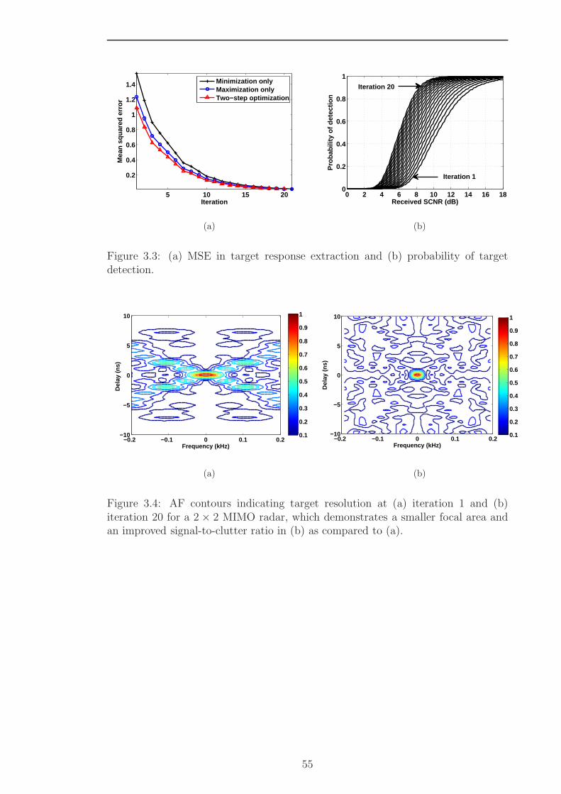
5 10 15 20

0.2

0.4

0.6

0.8

1

1.2

1.4

Iteration

Mea

n sq

uare

d er

ror

Minimization onlyMaximization onlyTwo−step optimization

(a)

0 2 4 6 8 10 12 14 16 180

0.2

0.4

0.6

0.8

1

Received SCNR (dB)

Pro

babi

lity

of d

etec

tion

Iteration 1

Iteration 20

(b)

Figure 3.3: (a) MSE in target response extraction and (b) probability of targetdetection.

Frequency (kHz)

Del

ay (

ns)

−0.2 −0.1 0 0.1 0.2−10

−5

0

5

10

0.1

0.2

0.3

0.4

0.5

0.6

0.7

0.8

0.9

1

(a)

Frequency (kHz)

Del

ay (

ns)

−0.2 −0.1 0 0.1 0.2−10

−5

0

5

10

0.1

0.2

0.3

0.4

0.5

0.6

0.7

0.8

0.9

1

(b)

Figure 3.4: AF contours indicating target resolution at (a) iteration 1 and (b)iteration 20 for a 2 × 2 MIMO radar, which demonstrates a smaller focal area andan improved signal-to-clutter ratio in (b) as compared to (a).

55

3.5 Chapter Summary

This chapter presents a two-stage waveform optimization algorithm for a cognitive

MIMO radar, which unifies the waveform design and selection procedures. The pro-

posed algorithm is based upon constant learning of the radar environment at the

transceiver and adaptation of the transmit waveforms to suit the non-stationary

radar scene. This ensures maximum information extraction from the target of in-

terest. Simulation results have demonstrated that the proposed approach results in

an improved performance in terms of target response estimation, target detection,

delay-Doppler resolution, and target discrimination.

56

(a)

Clutter

Target

(b)

Target

Clutter

(c)

Target

Clutter

(d)

0 0.02 0.04 0.06 0.08 0.10

0.2

0.4

0.6

0.8

1

Probability of false alarm

Pro

ba

bili

ty o

f d

ete

ctio

n

MIMO (Two step MI optimization)MIMO (MI maximization)SAR MIMO (MI minimization)CFAR

(e)

0 0.02 0.04 0.06 0.08 0.10

0.1

0.2

0.3

0.4

0.5

0.6

0.7

0.8

0.9

1

Probability of false alarm

Pro

ba

bili

ty o

f d

ete

ctio

n

MIMO (MI maximization)CFARSARMIMO (MI minimization)MIMO (Two step MI optimization)

(f)

Figure 3.5: (a) SAR image, (b) 4×4 MIMO radar (MI maximization), (c) 4×4 MIMOradar (MI minimization), and (d) 4× 4 MIMO radar two step MI optimization. (e)ROC for 2× 2 MIMO radar (f) ROC for 4× 4 MIMO radar.

57

0 2 4 6 8

02

46

80

0.2

0.4

0.6

0.8

1

x (m)y (m)

No

rma

lize

d

ba

cksca

tte

r sig

na

l

0.2

0.4

0.6

0.8

1

(a)

02

46

8

02

46

80

0.2

0.4

0.6

0.8

1

x (m)y (m)

No

rma

lize

db

acksca

tte

r sig

na

l

0.1

0.2

0.3

0.4

0.5

0.6

0.7

0.8

0.9

1

(b)

02

46

8

02

46

80

0.2

0.4

0.6

0.8

1

x (m)y (m)

No

rma

lize

d

ba

cksca

tte

r sig

na

l

0.1

0.2

0.3

0.4

0.5

0.6

0.7

0.8

0.9

1

(c)

0 5 10 15 200

0.5

1

1.5

Iterations

Mea

n sq

uare

d er

ror

Two step MI optimizationMI minimizationMI maximization

(d)

Figure 3.6: (a) Backscatter signal profile for MI minimization at iteration 20, (b)Backscatter signal profile for MI maximization at iteration 20, (c) Backscatter signalprofile for two-step waveform optimization at iteration 20, and (d) MSE performancefor 4× 4 MIMO configuration.

58

Chapter 4

Target Detection and Tracking

Using

Hidden-Markov-model-enabled

Cognitive Radar Network

In this chapter a novel HMM for describing the movement of an object, monitored

by a CRN, is developed. The problem of tracking the target is tackled using the

proposed HMM approach, which is integrated into the CRN that constantly learns

about its surroundings and adopts its operational mode accordingly. Both the re-

ceived signal strength (RSS) and time-of-arrival (TOA) of the backscatter signals

acquired at different radar units are applied to establish the HMM for characterizing

the non-stationary radar scene and enabling subsequent target detection and track-

ing. The system performance predicted using the proposed technique is then com-

pared to other widely-used algorithms including the EKF and maximum likelihood

estimation (MLE). Simulation results demonstrate the advantage of the proposed

cognitive tracking scheme as compared to the other approaches in terms of its higher

probability of detection and lower computational complexity, while maintaining the

same level of location accuracy.

59

4.1 Introduction

In wireless positioning systems, localization is usually achieved through the mea-

surement of relevant propagation parameters such as RSS, TOA, time-difference-of-

arrival (TDOA), and angle-of-arrival (AOA) [106–109]. Accurate ranging could be

obtained, in theory, by estimating RSS or TOA of the received waveforms. How-

ever, dense multipath and large delay spread, often found in indoor environments,

complicate the channel measurement process and deteriorate the performance of the

line-of-sight (LOS) signal acquisition. As a result, we use the hybrid RSS/TOA mea-

surements for localization instead of the conventional approach based upon RSS or

TOA only. On the other hand, the RSS information recorded at various radar com-

ponents is employed to construct the HMM for describing the dynamic radar scene

and subsequently enabling target detection and tracking. Specifically, the HMM

forms the basis of the adaptive learning module in the CRN, which continuously

collects the RSS/TOA information from the environment under surveillance and

estimates the HMM parameters responsible for generating the set of observations.

The target trajectory can then be estimated as an output of the HMM parameter

estimation process, which is fed back to the data fusion center for activation of the

nearby radars in accordance with the updated target location estimate. We will

consider UWB radars in the following discussions due to the high-resolution ranging

capability of UWB pulses [69, 110–113]. Nevertheless, the general methodology is

also applicable to any other types of radar waveforms.

HMM has been used for multiple target tracking applications in works like [114],

where superimposition of HMMs was applied. In [114], the parameters like target

location, velocity, etc. were classified as the underlying latent states for detection

through noisy observations. HMM was first applied to the problem of target local-

ization in [106]. However, the proposed HMM algorithm differs in the definition of

the Markov states and observations compared to those defined in [106]. The cur-

rent approach also differs from [106] in the way to perform spatial discretization of

the area under surveillance. In addition, we utilize a two-way propagation model

for radar signals, which is different from the one-way model for radio localization

in [106]. One possible solution for the target position and tracking estimation is the

one presented in [115] which has utilized particle filtering approach for tracking of

multiple targets within indoor localization scenarios. Other related contributions in

60

Table 4.1: Related WorksRelevant contributions References

CRN [34–36]

Application of CRN in object tracking [37]

HMM [118]

Application of HMM in indoor localization using RSS/TOA [106]

RSS/TOA based tracking with nonlinear system models [119]

indoor localization and tracking include [107, 110, 116, 117].

We build upon the ideas presented in Table 4.1, namely CRN [34–36] and its

application in object tracking [37], HMM [118] and its application in indoor localiza-

tion [106], and RSS/TOA based tracking [119], to propose a novel intelligent target

tracking platform.

The main contributions of this Chapter encompass the following aspects:

1. Development of a HMM-enabled CRN to detect and track an object by accu-

rately predicting the nearest radar units in an indoor environment; and

2. Evaluation of the probability of target detection and the root-mean-squared-

error (RMSE) of location estimate, and comparison of the results with the

benchmark algorithms including the EKF and the MLE.

4.2 Preliminaries of HMM-Enabled CRN

As indicated in Fig. 4.1, the target moves within a 2 D indoor environment and is

monitored using a CRN. As discussed in works like [37,106,119], a 2 D environment

is used to simplify the tracking problem under consideration. The height or the

azimuth information of the target is irrelevant to the radar scene under consideration,

since we are interested to locate the target within the 2D indoor map. This type of

approach is used for ground targets in which the radar units employ beam-steering

techniques to illuminate the radar scene in a direction parallel to the ground plane.

This greatly simplifies the problem since the spatial discretization need not be carried

out in a 3 D space. Each radar unit in the CRN is fixed at a known location and

transmits UWB pulses at fixed time intervals to probe the surroundings. The service

area under surveillance is divided into a number of Voronoi regions, where the radars

distributed in the region form the Voronoi centers as shown in Fig. 4.1. The locations

of the object are classified into discrete “states” following the Voronoi regions where

61

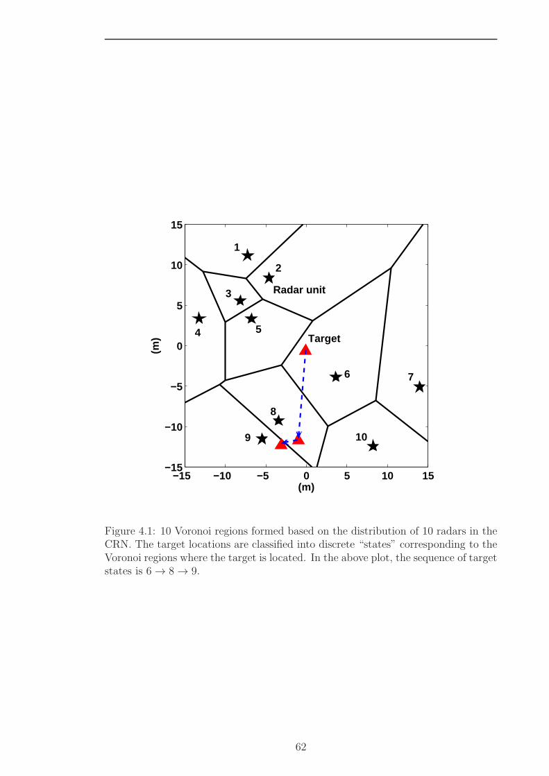
−15 −10 −5 0 5 10 15−15

−10

−5

0

5

10

15

(m)

(m)

Radar unit

Target

1

2

3

4 5

6 7

8

9 10

Figure 4.1: 10 Voronoi regions formed based on the distribution of 10 radars in theCRN. The target locations are classified into discrete “states” corresponding to theVoronoi regions where the target is located. In the above plot, the sequence of targetstates is 6 → 8 → 9.

62

Figure 4.2: System architecture of the HMM-enabled CRN.

the object is located. We further assume that the target states in consecutive time

instants are correlated.

A block diagram of the system architecture is illustrated in Fig. 4.2. Each radar

transmitter probes the environment to obtain a radar scene by sending UWB wave-

forms. The signals reflected from the target are sampled and the RSS/TOA profiles

are extracted, which are relayed to a central data fusion center. Subsequently, the

data fusion center stores the measurements recorded by all radars and constructs a

global RSS/TOA map. The global RSS/TOA map comprises the first arrived pulse

of the backscatter signal at each radar unit as well as the corresponding TOA lag.

It then identifies the nearest set of radars based upon this profile at the current

time instant to facilitate triangulation of the object. The index of the nearest radar

(or equivalently, the Voronoi region in which the target is located) is identified as

the state of the target to establish the HMM. Next, the data fusion center forwards

this information to the estimation and tracking module, which then estimates the

required HMM parameters. This process is repeated until the convergence of the

parameters is achieved. The estimation and tracking module then computes the

target position, which is fed back to the data fusion center and is subsequently used

for activating the appropriate group of radars in the vicinity of the object in the next

time interval. This operation facilitates adaptive illumination of the radar scene and

essentially leads to a CRN featuring the following two properties described in [34,35]:

(i) intelligent signal processing, which builds on real-time learning through contin-

uous interactions of the CRN with the surroundings; and (ii) feedback from the

63

receiver to the transmitter, which is a facilitator of intelligence.

We consider a monostatic radar configuration, where the transmitter and the

receiver are collocated. The radar channel comprises a forward connection and a

backward connection. The former describes signal propagation from the transmitter

to the target, while the latter characterizes the target-to-receiver link. Each radar

measures the RSS and TOA of the backscatter signal from the object. The method

of least square is then applied for location estimation from the noisy set of mea-

surements. To solve the multimodal optimization problem due to the nonlinearity

of the relationship between RSS/TOA and target position, the Taylor-series expan-

sion method is used to linearize the measurement model following the procedures

in [108, 109]. It is worth noting that a radio frequency identification (RFID) tag

could be attached to the object to enhance its radar cross section [37, 120, 121]. In

this case, a radar unit also serves as a RFID reader, and the RFID tag could facili-

tate boosting of the backscatter signal (e.g., enhanced RSS, more recognizable target

signature) from the target, potentially leading to improved localization accuracy.

It is assumed that each LOS path has been extracted through some preprocess-

ing steps. For example, each radar may employ beam-steering [37, 122] and delay

windowing [101] to suppress undesirable clutter interference. As a result, we focus

on the direct path in the subsequent analysis. The TOA is equal to the round-trip

propagation time τ = 2d/c, where d is the one-way propagation distance and c is

the speed of the electromagnetic wave. To account for the dependence of RSS on d,

the received power can be expressed as [120]

PR = −10α log τ + , (4.1)

where α is the two way path loss exponent, and = 10 logPT+K is a constant that

depends on the power PT of the transmit antenna and a propagation constant K

that depends on the indoor path loss model that we adopt. The value of α = 4.8 and

K = −25 dB is as shown in [123]. Thus (4.1) represents the log-normal shadowing

and fast fading effect for the received signal power. The received signal could also be

represented as where PT represents the transmission power, and α denotes the one-

way path loss exponent. The extension to noisy LOS data due to channel shadowing

and fading, imperfect LOS acquisition, and measurement errors can be realized by

modeling PR and τ as log-normal random variables as discussed in the subsequent

64

analysis.

4.3 HMM for Target Tracking

4.3.1 Problem Formulation

All radars are assumed to be randomly distributed in the service area, which is

divided into distinct Voronoi regions with each radar acting as the center. In the

beginning, the target is supposed to be equiprobable anywhere in the region. As

indicated in Fig. 4.1, the target makes random walks in the indoor environment.

Hence, the transition from one location to another is governed by the following

relationship

xt+1 = xt + νt. (4.2)

In (4.2), xt+1 and xt denote the position vectors at time instants t + 1 and t, re-

spectively. The term νt is a random perturbation at time t, which can be modeled

using various perturbation distributions as described in [106]. In the current work,

νt is assumed to follow a 2D Gaussian process. The following terms will be used

henceforth to characterize the HMM.

• Radar index defines the unique identity number assigned to each radar in the

CRN.

• State qt defines the Voronoi region where the target belongs, and is the same

as the index of the nearest radar at time t.

• Position vector xt defines the target location in the Cartesian coordinates at

time t.

• Trajectory XT , (x1,x2, · · · ,xT ) defines the sequence of position vectors from

time t = 1 to t = T .

• Observation sequence zt defines the sequence of quantized RSS levels observed

at time t (see also Fig. 4.3). Note that in order to simplify the analysis and

implementation, we only apply the RSS to establish the HMM. Nevertheless,

both the RSS and TOA data could be utilized through a 2D quantization of

the RSS-TOA space in Fig. 4.3.

65

• Transition matrix A defines the matrix of probabilities of transition between

states.

• Observation matrix B defines the matrix of probabilities of observing each

quantized RSS level given the state of the target.

• Initial state probability vector π defines the vector of probabilities of the initial

state where the target belongs.

• HMM parameter set λ defines the set of A and B.

The main objective is to establish the HMM model π and λ, which describes the

target trajectory in the environment. Once the model is developed, we can utilize

it to address the following two problems.

• Problem 1: Given λ, estimating the most probable set of target locations in

the next time instant.

• Problem 2: Optimizing λ by updating the parameters A and B at each time

instant.

Subsequently, a scheme utilizing both the training and prediction phases for the

HMM (see also the flowchart in Fig. 4.4) is developed. In the training phase, we

construct the HMM model. In the prediction phase, we address the two problems

mentioned above. A brief description of the Baum-Welch algorithm mentioned in

[118] in order to re-estimate the HMM parameters like the state transition matrix

A and the observation matrix B as a solution to Problem 2 is also presented. This

is achieved by using the newly observed data and old values of A and B.

4.3.2 Training Phase

During the training stage when the HMM model is being built, all the radar com-

ponents in the region are powered up to detect and locate the target by triangu-

lation [108, 109]. The state or the physical location of the target is treated as an

unknown (hidden) variable. The only observable part of the process is the backscat-

ter signal from the target.

Initially, the target under monitoring is supposed to be equiprobable in any state.

As the object changes from one state to another, its transitions are recorded during

66

the training phase. Based upon this learning process, the transition matrix A can

be constructed. For developing the observation matrix B, we discretize the RSS

at the nearest radar into distinct levels as illustrated in Fig. 4.3. Each RSS level

corresponds to a particular target-to-radar distance following (4.1). Subsequently,

the relative frequency of each level can be calculated by applying the entire set of

RSS samples associated with this specific Markov state (i.e., the index of the nearest

radar), which yields the probability of observation of each quantized RSS level.

Let M be the total number of states or equivalently, the number of radars in the

CRN; K be the number of quantized RSS levels; amn (m,n ∈ 1, 2, · · · ,M) be theprobability of transition from statem to state n, and bmk (m ∈ 1, 2, · · · ,M and k ∈1, 2, · · · , K) be the probability of observing the kth RSS level when the target is

in state m. The following relationships can be obtained:

amn =Number of transitions from state m to state n

Total number of transitions from state m,

bmk =Number of occurences of RSS level k when target is in state m

Total number of times when target is in state m.

The HMM model π and λ can thus be formulated as

π =

1M

...

1M

, A =

a11 · · · a1M...

. . ....

aM1 · · · aMM

, B =

b11 · · · b1K...

. . ....

bM1 · · · bMK

.

(4.3)

4.3.3 Prediction Phase

Once the HMM parameter set λ is derived, we can start utilizing the two matrices A

and B to predict the most probable set of target locations and RSS measurements.

Essentially, we attempt to solve both Problem 1 and Problem 2 during the prediction

phase.

4.3.3.1 Solution to Problem 1

Let ZT = (z1, z2, · · · , zT ) be the sequence of observations up to time T . The most

straightforward way of finding Pr(ZT |λ), where Pr(·) denotes probability, is through

67

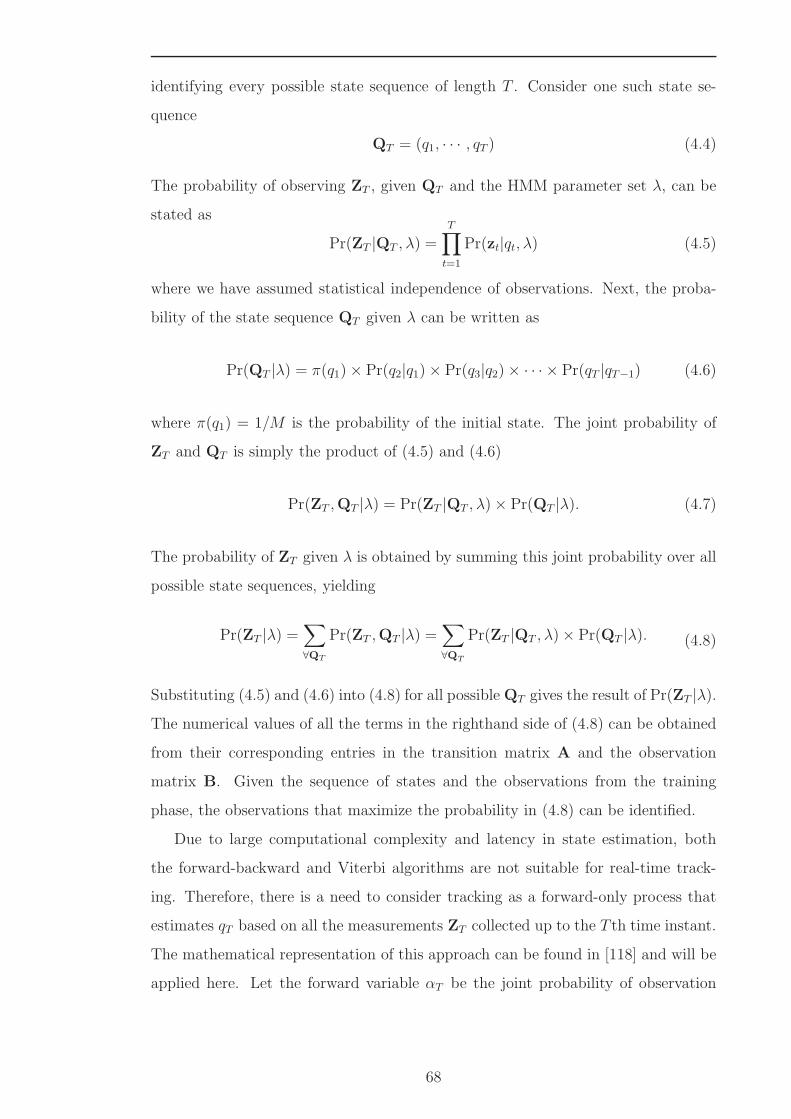
identifying every possible state sequence of length T . Consider one such state se-

quence

QT = (q1, · · · , qT ) (4.4)

The probability of observing ZT , given QT and the HMM parameter set λ, can be

stated as

Pr(ZT |QT , λ) =

T∏

t=1

Pr(zt|qt, λ) (4.5)

where we have assumed statistical independence of observations. Next, the proba-

bility of the state sequence QT given λ can be written as

Pr(QT |λ) = π(q1)× Pr(q2|q1)× Pr(q3|q2)× · · · × Pr(qT |qT−1) (4.6)

where π(q1) = 1/M is the probability of the initial state. The joint probability of

ZT and QT is simply the product of (4.5) and (4.6)

Pr(ZT ,QT |λ) = Pr(ZT |QT , λ)× Pr(QT |λ). (4.7)

The probability of ZT given λ is obtained by summing this joint probability over all

possible state sequences, yielding

Pr(ZT |λ) =∑

∀QT

Pr(ZT ,QT |λ) =∑

∀QT

Pr(ZT |QT , λ)× Pr(QT |λ). (4.8)

Substituting (4.5) and (4.6) into (4.8) for all possibleQT gives the result of Pr(ZT |λ).The numerical values of all the terms in the righthand side of (4.8) can be obtained

from their corresponding entries in the transition matrix A and the observation

matrix B. Given the sequence of states and the observations from the training

phase, the observations that maximize the probability in (4.8) can be identified.

Due to large computational complexity and latency in state estimation, both

the forward-backward and Viterbi algorithms are not suitable for real-time track-

ing. Therefore, there is a need to consider tracking as a forward-only process that

estimates qT based on all the measurements ZT collected up to the T th time instant.

The mathematical representation of this approach can be found in [118] and will be

applied here. Let the forward variable αT be the joint probability of observation

68

sequence ZT and state qT at time T ,

αT = Pr(ZT , qT |λ). (4.9)

The observation probability Pr(ZT |λ) is the summation of αT over all possible states,

viz.,

Pr(ZT |λ) =M∑

m=1

αT (m) =M∑

m=1

Pr(ZT , qT = m|λ) (4.10)

where αT (m) is the joint probability of ZT and qT = m. One possible optimality

criteria is to choose the state that is individually most likely. To implement this

solution, we define

γT (m) = Pr(qT = m|ZT , λ) (4.11)

which is the probability of the target being in state m at time T , given the observa-

tion sequence ZT and the HMM parameter set λ. Thus we can write (4.11) in the

form of the forward variables αT (m) as

γT (m) =αT (m)

Pr(ZT |λ)=

αT (m)∑M

m=1 αT (m). (4.12)

Using γT (m), we can solve for the individually most likely state m at time T as

m = argmaxm

[γT (m)] (4.13)

where m takes the values of 1, 2, · · · ,M .

Subsequently, the most probable zT and qT at time T can be identified from

(4.8) and (4.13) respectively, and with the help of A and B. This depends on our

knowledge of the trajectory until now through the sequence of states, QT , which we

assume to have since the prediction module follows the training phase and therefore

we are aware of these parameters. Using (4.13) we can predict the most likely state

m during the next time instant. The predicted future state and the observation

matrix B can be utilized to find out the most probable RSS level. Finally, the

target distance from the nearest radar in the next time instant can be predicted.

Thus the current illumination strategy can be designed in accordance with this

prediction to address Problem 1.

69

4.3.3.2 Solution to Problem 2

In this problem, we wish to optimize the parameters, A and B of the HMM model.

Before each instance of reception, the HMM algorithm predicts the most probable

target location and accordingly illuminates the target scene. Since we aim at op-

timizing the HMM parameters at every iteration, the error in prediction does not

propagate. The approach towards optimization of λ was introduced in [118] and

termed as the Baum-Welch algorithm. As shown in (4.11) and (4.12),

γT (m) = Pr(qT = m|ZT , λ) =αT (m)

∑M

m=1 αT (m). (4.14)

We also define the quantity

ξmn(T ) = Pr(qT = m, qT+1 = n|ZT , λ) (4.15)

which is the probability of being in state m at time T and being in state n at time

T + 1. ξmn can also be expanded as

ξmn(T ) =Pr(qT = m, qT+1 = n,ZT |λ)

Pr(ZT , λ). (4.16)

Thus

ξmn(T ) =Pr(ZT , qT = m|λ)amnPr(ZT , qT+1 = n|λ)

∑Nm=1

∑Nn=1Pr(ZT , qT = m|λ)amnPr(ZT , qT+1 = n|λ)

. (4.17)

In order to estimate the new parameters for the HMM using the old parameters

and the data, we can simplify the relative frequencies as follows

πm = γ1(m) (4.18)

which is the expected relative frequency spent in state m at time T = 1. The

updated transition probability

amn =

∑Tt=1 ξmn(t)∑Tt=1 γt(m)

(4.19)

which is the expected number of transitions from state m to state n relative to the

expected total number of transitions from state m. This can be used to update the

70

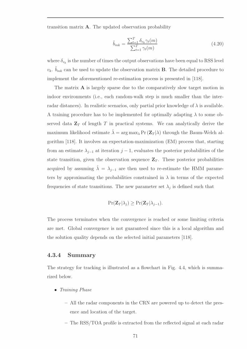
transition matrix A. The updated observation probability

bmk =

∑Tt=1 δvkγt(m)∑T

t=1 γt(m)(4.20)

where δvk is the number of times the output observations have been equal to RSS level

vk. bmk can be used to update the observation matrix B. The detailed procedure to

implement the aforementioned re-estimation process is presented in [118].

The matrix A is largely sparse due to the comparatively slow target motion in

indoor environments (i.e., each random-walk step is much smaller than the inter-

radar distances). In realistic scenarios, only partial prior knowledge of λ is available.

A training procedure has to be implemented for optimally adapting λ to some ob-

served data ZT of length T in practical systems. We can analytically derive the

maximum likelihood estimate λ = argmaxλ Pr (ZT |λ) through the Baum-Welch al-

gorithm [118]. It involves an expectation-maximization (EM) process that, starting

from an estimate λj−1 at iteration j − 1, evaluates the posterior probabilities of the

state transition, given the observation sequence ZT . These posterior probabilities

acquired by assuming λ = λj−1 are then used to re-estimate the HMM parame-

ters by approximating the probabilities constrained in λ in terms of the expected

frequencies of state transitions. The new parameter set λj is defined such that

Pr(ZT |λj) ≥ Pr(ZT |λj−1).

The process terminates when the convergence is reached or some limiting criteria

are met. Global convergence is not guaranteed since this is a local algorithm and

the solution quality depends on the selected initial parameters [118].

4.3.4 Summary

The strategy for tracking is illustrated as a flowchart in Fig. 4.4, which is summa-

rized below.

• Training Phase

– All the radar components in the CRN are powered up to detect the pres-

ence and location of the target.

– The RSS/TOA profile is extracted from the reflected signal at each radar

71

and is sent to the central data fusion center.

– The data fusion center identifies the set of four radars closest to the

object (which include the nearest one indicating the “state” of the target

location) from the gathered RSS/TOA profiles.

– The set of four nearest radars are used to triangulate the position of

the target by applying the methods of least square and Taylor series

expansion [108, 109]. This information is used to build the HMM.

– The preceding steps are repeated until the convergence of the HMM pa-

rameters is achieved.

• Prediction Phase

– Once the training phase is completed, the system makes predictions about

the future target location and the corresponding set of radars in the

vicinity. This prior knowledge of the nearest radars facilitates stimulation

of only those nearby radars in the next time instant.

– Based on the values of A and B estimated during the training phase,

four nearest radars are deduced by the data fusion center. The four

radar units collect the first arrived backscatter signal as shown in the

RSS/TOA profile in Fig. 4.3.

– The data fusion center then detects the presence of the target by com-

paring the RSS values with a pre-specified threshold, and triangulates

its position based on the RSS/TOA profiles, which are collected from

the radars activated in the previous step. Any error in estimation of

the target state is identified by the fusion center based upon the latest

RSS/TOA profiles and is used to update the transition matrix and the

observation matrix in the HMM. The process of estimating the nearest

four radars is also repeated. In this way adaptability is incorporated in

the CRN.

During the entire tracking process, the overall power transmitted by the CRN to

probe the surroundings is fixed and equally parceled out to the activated radars.

In the next section, we will evaluate the Cramer-Rao Lower Bound (CRLB) on

the estimation of the target position using the RSS/TOA profiles and analyze the

72

convergence of the proposed HMM algorithm. Other works like [124] and [125]

have derived the CRLB on RSS/TOA measurements. We use a similar approach to

establish the CRLB for our case to gauge the RMSE performance of the HMM and

other tracking algorithms.

4.4 Theoretical Analysis

4.4.1 CRLB on Location Error

At an arbitrary time instant, let us define the observed RSS/TOA profile Θ to be

Θ = (τ1, τ2, τ3, · · · , τM , P1, P2, P3, · · · , PM) (4.21)

where τm and Pm (m = 1, 2, · · · ,M) are the TOA and RSS of the backscatter signals

at the mth radar.

Define the actual location of the target in the Cartesian coordinates as ψ0 =

(x0, y0). The positioning problem then consists of finding an estimate of ψ0, ψ0, given

the vector of the radar locations Ψ = [Ψ1, · · · ,ΨM ], where Ψm = (xm, ym) (m =

1, 2, · · · ,M) gives the Cartesian coordinates of the mth radar. To obtain a lower

bound on the estimation error, we assume that the TOA and RSS measurements

are independent. This is because correlation in measured data usually reduces the

degrees of freedom and thus increases the positioning error. Furthermore, the pdf

of TOAs is assumed to follow τm ∼ N(2dm/c, σ2τ ), where N indicates the normal

distribution, dm is the distance between the mth radar and the target, c is the

speed of the electromagnetic wave, and στ is the parameter describing the joint

nuisance of the channel estimation and measurement errors. The RSSs are supposed

to be lognormal random variables with Pm ∼ N(PR,m(dB), σ2P ), where PR,m(dB) =

P0(dB)−20α log10(dm)+20α log10 d0 following (4.1) and σP is the standard deviation

of lognormal shadowing.

The CRLB of an unbiased estimator ψ0 is given by the inverse of the Fisher

information matrix (FIM), which has the form

I(ψ0) = −E ∇ψ0(∇ψ0

L (Θ|ψ0,Ψ))

=

Ixx Ixy

Ixy Iyy

(4.22)

73

where ∇ψ0denotes the derivative with respect to ψ0, E· is the expectation oper-

ator, and L(Θ|ψ0,Ψ) is the logarithm of the conditional pdf

L(Θ|ψ0,Ψ) =M∑

m=1

ln[fτm|ψ0,Ψm

(τm|ψ0,Ψm)]+

M∑

m=1

ln[fPm|ψ0,Ψm

(Pm|ψ0,Ψm)].

(4.23)

Subsequently, Ixx is derived as

Ixx = −M∑

m=1

E

∂2

∂x20ln[fτm|ψ0,Ψm

(τm|ψ0,Ψm)]

−M∑

m=1

E

∂2

∂x20ln[fPm|ψ0,Ψm

(Pm|ψ0,Ψm)]

.

(4.24)

The other two terms Ixy and Iyy can be similarly computed. Subsequently, the

CRLB on the variance of the RSS/TOA location estimation is given by

σ2ψ0

=Ixx + Iyy

IxxIyy − I2xy. (4.25)

A detailed derivation of the CRLB can be found in [125].

Following [125], the FIM for our case can be expressed as

I(ψ0) =

1c2σ2τ

∑M

m=1(x0−xm)2

d2m

+Υ∑M

m=1(x0−xm)2

d4m

1c2σ2τ

∑M

m=1(x0−xm)(y0−ym)

d2m

+Υ∑M

m=1(x0−xm)(y0−ym)

d4m

1c2σ2τ

∑Mm=1

(x0−xm)(y0−ym)d2m

+Υ∑M

m=1(x0−xm)(y0−ym)

d4m

1c2σ2τ

∑Mm=1

(y0−ym)2

d2m

+Υ∑M

m=1(y0−ym)2

d4m

(4.26)

where Υ =(

20ασP ln 10

)2. Using (4.24) and (4.25), σ2

ψ0can be determined. It is worth

noting that the CRLB is proportional to the factor Υ linked to RSS measurements

and also proportional to 1/ (c2σ2τ ) linked to TOA measurements. The CRLB also

depends upon the number of the radars, M .

4.4.2 Convergence of the HMM Algorithm

The HMM parameters A and B can be optimized using the Baum-Welsh algorithm

or the EM algorithm as stated in [118]. Each iteration of the EM algorithm consists

of two stages: the expectation step (E-step) and the maximization step (M-step). In

the E-step, the missing data are estimated given the observed data and the current

74

estimate of the model parameters. This is achieved using the expectation. In the

M-step, the likelihood function is maximized under the assumption that the missing

data are known. The results acquired from the E-step are used in lieu of the actual

missing data.

Let Z be the sequence of RSS observations at an arbitrary time. In order to

estimate the parameter set λ representing A and B, it is typical to introduce the

log-likelihood function defined as

L(λ) = ln [Pr(Z|λ)] . (4.27)

Since ln(·) is a strictly increasing function, the value of λ that maximizes Pr(Z|λ)also maximizes L(λ). The EM algorithm is an iterative procedure for maximizing

L(λ). Assume that after the (j − 1)th iteration the current estimate for λ is given

by λj−1. Since the objective is to maximize L(λ), we wish to compute an updated

estimate λj such that,

L(λj) ≥ L(λj−1). (4.28)

By determining the conditional expectation of the unobserved likely states q (which

are the missing data) and maximizing it with respect to λ, the local convergence is

guaranteed as it increases the likelihood at each iteration. A detailed discussion on

the convergence properties of the EM algorithm is presented in [126]. For the sake

of completeness, we provide a brief analysis of the convergence of the algorithm in

the current context of target tracking.

We aim at maximizing the difference as indicated in (4.27),

L(λj)− L(λj−1) = ln [Pr(Z|λj)]− ln [Pr(Z|λj−1)] . (4.29)

Denote the likely state of the moving target as q, which corresponds to the Voronoi

region where the target is located, as shown in Fig. 4.1. q is considered to be

the hidden or unobserved variable in both the HMM and EM algorithm setting.

75

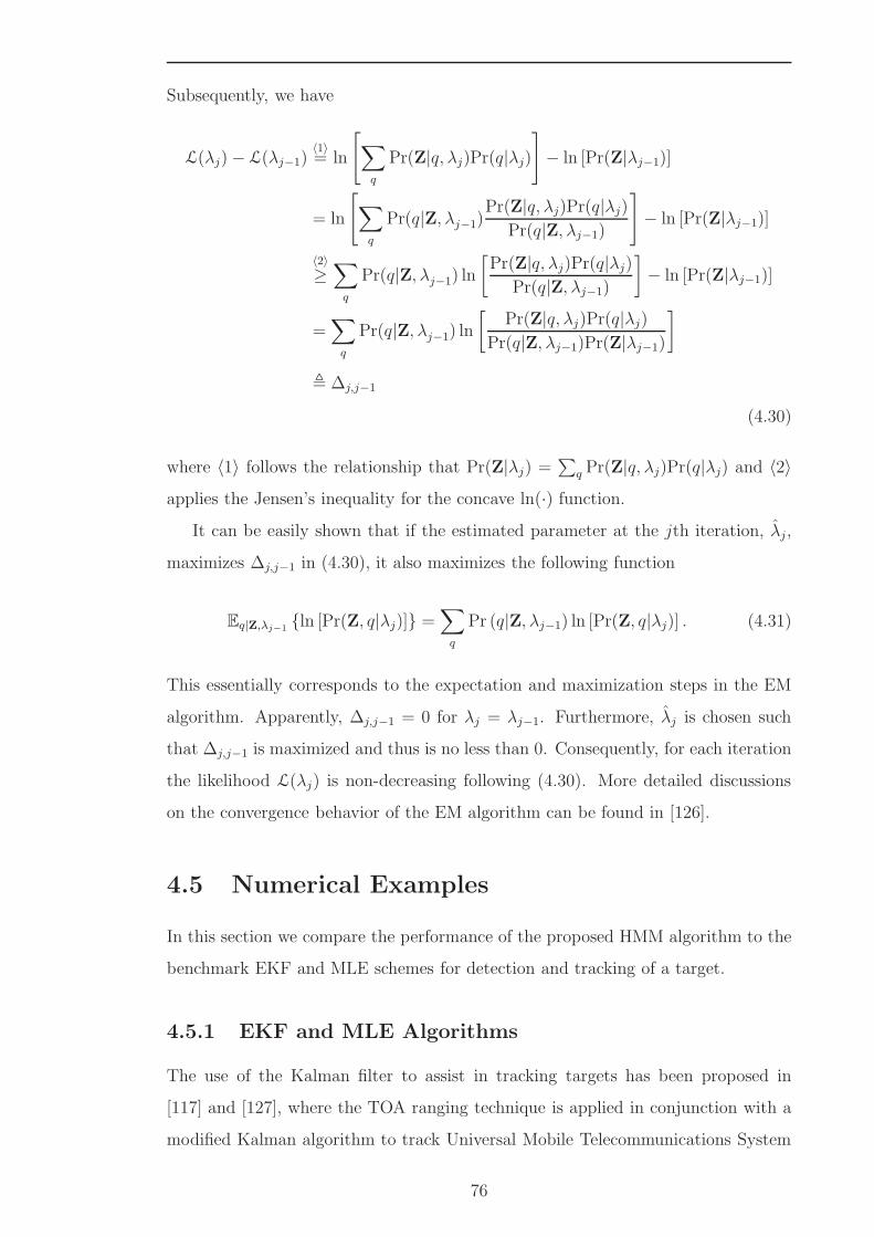
Subsequently, we have

L(λj)− L(λj−1)〈1〉= ln

[∑

q

Pr(Z|q, λj)Pr(q|λj)]− ln [Pr(Z|λj−1)]

= ln

[∑

q

Pr(q|Z, λj−1)Pr(Z|q, λj)Pr(q|λj)

Pr(q|Z, λj−1)

]− ln [Pr(Z|λj−1)]

〈2〉

≥∑

q

Pr(q|Z, λj−1) ln

[Pr(Z|q, λj)Pr(q|λj)

Pr(q|Z, λj−1)

]− ln [Pr(Z|λj−1)]

=∑

q

Pr(q|Z, λj−1) ln

[Pr(Z|q, λj)Pr(q|λj)

Pr(q|Z, λj−1)Pr(Z|λj−1)

]

, ∆j,j−1

(4.30)

where 〈1〉 follows the relationship that Pr(Z|λj) =∑

q Pr(Z|q, λj)Pr(q|λj) and 〈2〉applies the Jensen’s inequality for the concave ln(·) function.

It can be easily shown that if the estimated parameter at the jth iteration, λj,

maximizes ∆j,j−1 in (4.30), it also maximizes the following function

Eq|Z,λj−1ln [Pr(Z, q|λj)] =

∑

q

Pr (q|Z, λj−1) ln [Pr(Z, q|λj)] . (4.31)

This essentially corresponds to the expectation and maximization steps in the EM

algorithm. Apparently, ∆j,j−1 = 0 for λj = λj−1. Furthermore, λj is chosen such

that ∆j,j−1 is maximized and thus is no less than 0. Consequently, for each iteration

the likelihood L(λj) is non-decreasing following (4.30). More detailed discussions

on the convergence behavior of the EM algorithm can be found in [126].

4.5 Numerical Examples

In this section we compare the performance of the proposed HMM algorithm to the

benchmark EKF and MLE schemes for detection and tracking of a target.

4.5.1 EKF and MLE Algorithms

The use of the Kalman filter to assist in tracking targets has been proposed in

[117] and [127], where the TOA ranging technique is applied in conjunction with a

modified Kalman algorithm to track Universal Mobile Telecommunications System

76

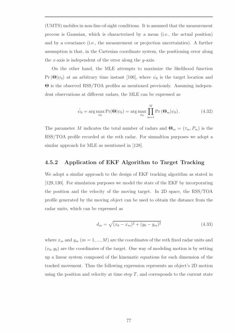
(UMTS) mobiles in non-line-of-sight conditions. It is assumed that the measurement

process is Gaussian, which is characterized by a mean (i.e., the actual position)

and by a covariance (i.e., the measurement or projection uncertainties). A further

assumption is that, in the Cartesian coordinate system, the positioning error along

the x-axis is independent of the error along the y-axis.

On the other hand, the MLE attempts to maximize the likelihood function

Pr (Θ|ψ0) at an arbitrary time instant [106], where ψ0 is the target location and

Θ is the observed RSS/TOA profiles as mentioned previously. Assuming indepen-

dent observations at different radars, the MLE can be expressed as

ψ0 = argmaxψ0

Pr(Θ|ψ0) = argmaxψ0

M∏

m=1

Pr (Θm|ψ0) . (4.32)

The parameter M indicates the total number of radars and Θm = (τm, Pm) is the

RSS/TOA profile recorded at the mth radar. For simualtion purposes we adopt a

similar approach for MLE as mentioned in [128].

4.5.2 Application of EKF Algorithm to Target Tracking

We adopt a similar approach to the design of EKF tracking algorithm as stated in

[129,130]. For simulation purposes we model the state of the EKF by incorporating

the position and the velocity of the moving target. In 2D space, the RSS/TOA

profile generated by the moving object can be used to obtain the distance from the

radar units, which can be expressed as

dm =√(x0 − xm)2 + (y0 − ym)2 (4.33)

where xm and ym (m = 1, ...,M) are the coordinates of themth fixed radar units and

(x0, y0) are the coordinates of the target. One way of modeling motion is by setting

up a linear system composed of the kinematic equations for each dimension of the

tracked movement. Thus the following expression represents an object’s 2D motion

using the position and velocity at time step T , and corresponds to the current state

77

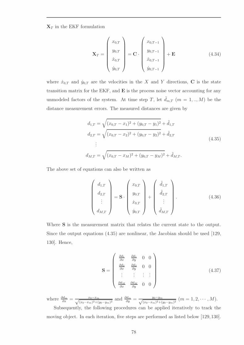
XT in the EKF formulation

XT =

x0,T

y0,T

x0,T

y0,T

= C ·

x0,T−1

y0,T−1

x0,T−1

y0,T−1

+ E (4.34)

where x0,T and y0,T are the velocities in the X and Y directions, C is the state

transition matrix for the EKF, and E is the process noise vector accounting for any

unmodeled factors of the system. At time step T , let dm,T (m = 1, ..,M) be the

distance measurement errors. The measured distances are given by

d1,T =√(x0,T − x1)2 + (y0,T − y1)2 + d1,T

d2,T =√(x0,T − x2)2 + (y0,T − y2)2 + d2,T

...

dM,T =√(x0,T − xM )2 + (y0,T − yM)2 + dM,T .

(4.35)

The above set of equations can also be written as

d1,T

d2,T...

dM,T

= S ·

x0,T

y0,T

x0,T

y0,T

+

d1,T

d2,T...

dM,T

. (4.36)

Where S is the measurement matrix that relates the current state to the output.

Since the output equations (4.35) are nonlinear, the Jacobian should be used [129,

130]. Hence,

S =

∂d1∂x

∂d1∂y

0 0

∂d2∂x

∂d2∂y

0 0...

......

...

∂dM∂x

∂dM∂y

0 0

(4.37)

where ∂dm∂x

= x0−xm√(x0−xm)2+(y0−ym)2

and ∂dm∂y

= y0−ym√(x0−xm)2+(y0−ym)2

(m = 1, 2, · · · ,M).

Subsequently, the following procedures can be applied iteratively to track the

moving object. In each iteration, five steps are performed as listed below [129,130].

78

1. Project the state ahead: X−T = C ·XT−1;

2. Project the error covariance ahead: W−T = C ·WT−1 ·CT +Ω;

3. Evaluate the Kalman gain: KT = W−T · ST ·

(S ·W−

T · ST +R)−1

;

4. Update estimation with measurements: XT = X−T +KT ·

(DT − S ·X−

T

);

5. Update the error covariance: WT = (I−KT · S) ·W−T .

In Step 1, the current state XT−1 is used to estimate the location at the next time

instant. The error covariance matrixW−T in the next time step is projected using the

state space model C and the process noise covariance matrix Ω in Step 2, where (·)T

denotes the matrix transpose. In Step 3, the Kalman gain KT is computed, where R

is a diagonal matrix representing the independent distance measurement noises at

different radars. The Kalman gain is used in Step 4, when the distance measurements

DT = [d1,T , d2,T , · · · , dM,T ]T from the radars to the target are employed to update

the state, XT . In Step 5, the error covariance matrix WT is updated. The current

position (x0,T , y0,T ) is readily available from the state XT .

In the simulation study of the EKF algorithm presented previously, the same area

under surveillance of dimensions 30 m×30 m was chosen with the same distribution

of radar units as illustrated in Fig. 4.1. The sampling time or the time step was

chosen to be 1 ms. The step size standard deviation of the target trajectory was set

to be σν = 50 cm. The process noise covariance matrix Ω, the state space model C,

and the measurement noise matrix R were assumed to be

Ω =

400 cm2 0 0 0

0 400 cm2 0 0

0 0 100 cm2/s2 0

0 0 0 100 cm2/s2

,

C =

1 0 1 ms 0

0 1 0 1 ms

0 0 1 0

0 0 0 1

,

R =

10 cm · · · 0...

. . ....

0 · · · 10 cm

.

79

Table 4.2: Simulation Setup: Radar PositionsRadar index x position (m) y position (m)

Radar 1 −7.239 11.15Radar 2 −4.593 8.387Radar 3 −8.158 5.565Radar 4 −13.21 3.367Radar 5 −6.78 3.328Radar 6 3.636 −3.874Radar 7 13.96 −5.094Radar 8 −3.42 −9.268Radar 9 −5.455 −11.52Radar 10 8.237 −12.43

4.5.3 Simulation Results

Simulations have been carried out to evaluate the performance of the HMM algo-

rithm with regards to the probability of detection, the RMSE for target tracking,

and the CRLB on RSS/TOA localization. The probing radar waveforms are Gaus-

sian monocycles with a central frequency of 4 GHz at a bandwidth of 700 MHz

and the sampling frequency used is 10 GHz. The acquisition time for RSS/TOA

acquisition is set to be 0.01 ms. The layout of the CRN under consideration is illus-

trated in Fig. 4.1, where 10 radar units are normally distributed in a 30 m× 30 m

region. The observation space of RSS levels has been fixed for simulation purposes

and has a value of K = 6. The target makes random walks in the service area,

where each step follows a normal distribution with a standard deviation of 50 cm.

The sampling time for RSS/TOA acquisition has been selected to be small enough

to cater to the target movement. Finally, the one-way path loss exponent is chosen

to be α = 2.4 following the value suggested in [131]. We assume that the radar

units operate asynchronously. In the case of a synchronous operation of different

radars, various orthogonal maximum length UWB sequences (see e.g., [132]) can

be employed to handle the interference rather than using a single pulse at distinct

radars. The radar positions for the simulation setup are as shown in Table 4.2 and

Fig. 4.1. The simulations are carried out by fixing the number and positions of the

radar units and varying the target trajectory.

Once the training phase is completed and the HMM model is constructed, sub-

sequent locations of the target are estimated using the proposed HMM algorithm

as well as the benchmark EKF and MLE algorithms. The probability of detection

is evaluated for various Signal to Noise Ratio (SNR) values ranging from 5 dB to

80

20 dB. In the HMM algorithm, only the radar units in the vicinity of the target

are activated, which is based upon prediction of the nearest radar. For the EKF

and MLE algorithms all the radar units are powered up. Based upon the target

position estimates made by the three tracking algorithms, the received signal is es-

timated and a hypothesis testing approach is used to compare the signal amplitude

with a pre-specified threshold value for detecting the presence of the target. This

threshold is determined by fixing the probability of false alarm at Pfa = 0.0001.

Following the Neyman-Pearson algorithm [2], we can calculate the threshold value

to be ε =√nσ2Q−1(Pfa), where σ

2 is the variance of the normalized received signal

amplitude, n is the number of samples, and Q is the complementary error function.

If we assume that the noise floor σ2 = 0.01, then the threshold translates into the

value of 0.3 V for a single normalized signal sample. To combine the binary decisions

made at different radars about the presence or absence of a target, the majority rule

is adopted. Fig. 4.5 is a result of averaging over 100 simulations each at a particular

SNR value. It demonstrates that as the SNR increases, the probability of target de-

tection is improved. In the case of the HMM algorithm, the probability of detection

is superior since only the nearby radar units are activated, thus avoiding the noise

contributions of distant radar components.

The RMSE of the target location is evaluated in Fig. 4.6(a). At each random-

walk step, the error in the location estimation is calculated. It can be seen that the

EKF and MLE algorithms achieve better target localization accuracy. This is due to

the fact that the EKF and MLE algorithms have superior degrees of freedom in terms

of the activated radar units. The parameters of the proposed HMM algorithm have

to be estimated at each step simultaneously with the location of the target, which

affects its RMSE performance. Nevertheless, as the random-walk step increases, the

achievable accuracy for all the three algorithms is similar and less than 1 m, which

is acceptable for indoor positioning applications as indicated in [133].

We evaluate the CRLB for the RSS/TOA based localization using (4.24) and

(4.25), which serves as a benchmark for comparison of the RMSE accuracy of the

tracking algorithms under consideration. In the current work, the data fusion center

selects the set of four nearest radar units for target localization. Hence, we consider

four radars placed at the following four locations: (−10 m,−10 m), (10 m,−10 m),

(−10 m, 10 m), and (10 m, 10 m), which synthesizes the scenario that a set of

close-by radars are activated for target positioning. As shown in Fig. 4.6(b), at

81

Table 4.3: Execution Times for Various Tracking AlgorithmsTracking algorithm Probability of detection > 0.9 RMSE < 0.3 m

σν = 10 cm σν = 20 cm σν = 50 cm σν = 10 cm σν = 20 cm σν = 50 cm

MLE 220 ms 240 ms 310 ms 200 ms 275 ms 325 ms

EKF 337 ms 350 ms 376 ms 309 ms 329 ms 345 ms

HMM 105 ms 127 ms 157 ms 308 ms 335 ms 357 ms

the central locations the maximum achievable accuracy is around 0.019 m, and the

CRLB reduces as the target moves towards one of the radar units.

Table 4.3 indicates the execution times for the three tracking algorithms under

consideration. The radar units are activated every 1 ms and the probability of

successful target detection is evaluated over an epoch of 50 such activations. The

simulation is repeated for various values of σν , which is the standard deviation

defining the step size of the 2D motion of the target. The time demanded to achieve

a probability of detection greater than 0.9 for each of the tracking techniques is

evaluated over subsequent epochs. The HMM method displays the fastest detection

of the target due to its ability to spatially discretize the area under surveillance.

A similar analysis is carried out with respect to the execution time required to

achieve a RMSE < 0.3 m. In this case, the performance for the three algorithms is

similar particularly at larger σν , though the HMM algorithm requires slightly longer

execution times as compared to the EKF and MLE approaches.

Finally, we study the performance of the three techniques if only the nearest

set of radar units are activated for all the algorithms. Specifically, we look into the

influence of standard deviation of the step size σν on the RMSE, where σν is resolved

into two components, σνx and σνy along the X and Y directions, respectively. As

shown in Fig. 4.7, the HMM yields the least RMSE for higher values of σν as

compared to the EKF and MLE when all the algorithms have the same degrees

of freedom in terms of the activated radars. Furthermore, the performance of the

EKF and MLE for target position estimation is sensitive to the increase in the step

size. In other words, they are suboptimal for tracking rapid target movements. The

HMM algorithm on the other hand gains advantage from the spatial discretization

of the area under surveillance and hence, its performance will not be affected even if

there is an increase in the target velocity. These observations justify the use of the

HMM algorithm over the other two techniques for tracking fast target movements,

and also prove that intelligent illumination of the target scene alone is necessary but

82

not sufficient for achieving an enhanced RMSE performance.

Fig. 4.8 gives an illustrative example for the initialization of A and B as well as

their values after the training phase is completed. This example corresponds to an

arbitrary five-state HMM with six RSS levels of observation. As shown in Fig. 4.8,

the state transition matrix A is initialized with all states being equiprobable and

the observation matrix B is initialized with all observation levels being equiprobable

for each state. After achieving the convergence of A and B, each current state is

most likely to remain in the same state in the next time instant.

83

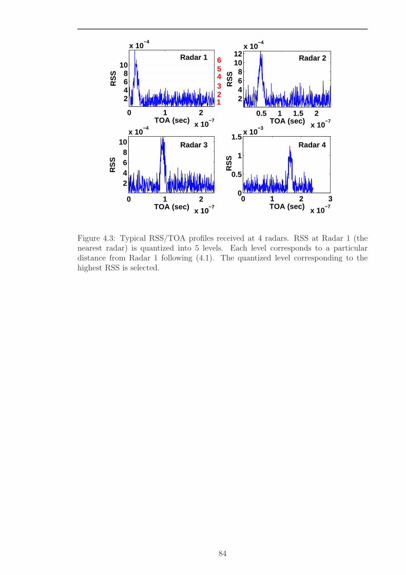
0 1 2

x 10−7

2468

10

x 10−4

TOA (sec)R

SS

0.5 1 1.5 2

x 10−7

2468

1012

x 10−4

TOA (sec)

RS

S

0 1 2

x 10−7

2468

10x 10

−4

TOA (sec)

RS

S

0 1 2 3

x 10−7

0

0.5

1

1.5x 10

−3

TOA (sec)

RS

S

Radar 1 Radar 2

Radar 3 Radar 4

123456

Figure 4.3: Typical RSS/TOA profiles received at 4 radars. RSS at Radar 1 (thenearest radar) is quantized into 5 levels. Each level corresponds to a particulardistance from Radar 1 following (4.1). The quantized level corresponding to thehighest RSS is selected.

84

Figure 4.4: Flowchart for the HMM-based target tracking algorithm.

85

5 8 11 14 17 200

0.2

0.4

0.6

0.8

1

SNR (dB)P

roba

bilit

y of

det

ectio

n

HMMMLEEKF

Figure 4.5: Probability of detection for various target tracking algorithms.

0 200 400 600 800 10000

0.2

0.4

0.6

0.8

1

1.2

Steps

RM

SE

(m

)

HMMEKFMLE

(a)

−10 −5 0 5 10−10

010

0.015

0.016

0.017

0.018

0.019

X (m)Y (m)

CR

LB (

m)

(b)

Figure 4.6: (a) Location estimation errors for various target tracking algorithms,(b) CRLB on RSS/TOA localization

86

Figure 4.7: RMSE performance of the 3 tracking algorithms with respect to varyingvalues of σνx and σνy .

87

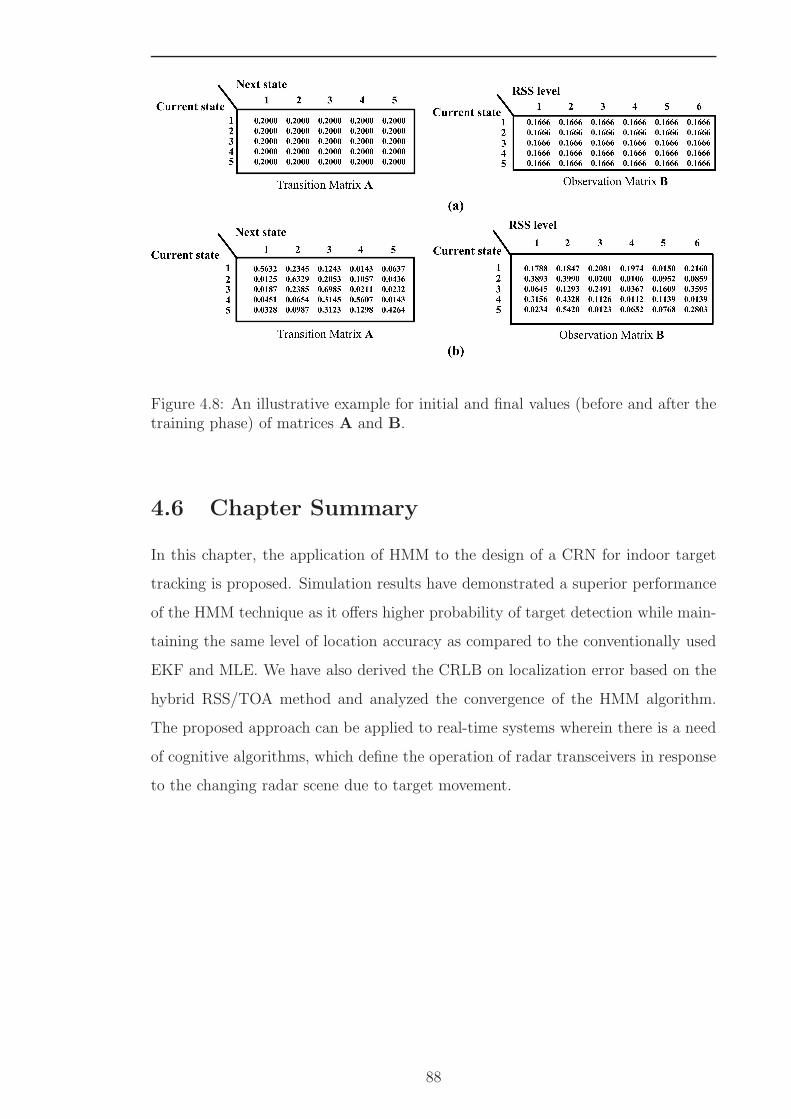
Figure 4.8: An illustrative example for initial and final values (before and after thetraining phase) of matrices A and B.

4.6 Chapter Summary

In this chapter, the application of HMM to the design of a CRN for indoor target

tracking is proposed. Simulation results have demonstrated a superior performance

of the HMM technique as it offers higher probability of target detection while main-

taining the same level of location accuracy as compared to the conventionally used

EKF and MLE. We have also derived the CRLB on localization error based on the

hybrid RSS/TOA method and analyzed the convergence of the HMM algorithm.

The proposed approach can be applied to real-time systems wherein there is a need

of cognitive algorithms, which define the operation of radar transceivers in response

to the changing radar scene due to target movement.

88

Chapter 5

Novel System Architecture and

Waveform Design for Cognitive

Radar Radio Networks

In this chapter, a novel approach to combining communication and radar function-

alities in a single waveform design for CRR networks is proposed. This approach

aims at extracting the target parameters from the radar scene, as well as facilitating

high-data-rate communications between CRR nodes by adopting a single waveform

optimization solution. The system design technique aims at addressing the coexist-

ing communication and radar detection problems in mission-critical services, where

there is a need of integrating the knowledge about the target scene gained from

distinct radar entities functioning in tandem with each other. The high spatial res-

olution and immunity to multipath fading make UWB signals an appropriate choice

for such applications. The proposed solution is achieved by applying the MI based

strategy to design the sequence of UWB transmission pulses and embed into them

the communication data with the pulse position modulation (PPM) scheme. With

subsequent iterations of the algorithm, simulation results demonstrate an improve-

ment in extraction of the parameters from the radar scene such as target position

and impulse response, while still maintaining high-throughput radio links with low

bit error rates (BERs) between CRR nodes.

89

5.1 Introduction

5.1.1 Background on Cognitive Radar Waveform Design and

Joint Communication-Radar Systems

In a cognitive radar, the information of the target scene parameters is relayed to

the transmitter by the receiver through a continuous feedback loop, which allows

the development of waveform design techniques that offer better target resolution

capabilities [132]. Excitation pulses can be optimized by application of information

theory to radar signal processing. Bell [3] studied the design of waveforms in the

context of illumination of extended targets for target detection and information

extraction. Yang and Blum [134] extended the work of Bell [3] by using MI as a

waveform optimization criterion subject to the limited transmission power in the

MIMO radar configuration.

The work in [134] in particular focuses upon the problem of radar waveform

design for target classification and identification, where the conditional MI between

the random target impulse response and the reflected signals is maximized given

the knowledge of the transmitted signals. Another problem that [135] addresses is

the design of waveforms based on minimization of mean square error (MMSE) in

estimating the target response. Analysis in [135] indicates that the above mentioned

two problems lead to the same waveform solution. The work in [132] focuses upon

designing UWB transmission waveforms with an aim of minimizing the MI between

the received radar pulses at successive instants of time. This is achieved by designing

the probing signals that will result in independent responses from the target scene in

a bid to gain more knowledge about the changing target parameters at each instant

of time.

In this chapter, we try to develop a novel cognitive architecture for the joint

communication-radar waveform design. Before we describe the actual architecture,

we provide a general background on the existing proposal of joint communication-

radar networks.

In recent years, the research in integrating the communication and radar system

designs under a common platform has gained significant momentum [24,25,28]. Such

a joint radar and communication system would constitute a unique cost-efficient

solution for future intelligent surveillance applications, for which both environmental

90

sensing and establishment of ad hoc communication links is essential.

Recent contributions such as [24] and [25] in particular focus upon the devel-

opment of devices that have multiple radio functions and combine communication

and radar in a small portable form with ultra-low power consumption. These works

have adopted the OFDM techniques fused with UWB technologies to realize the

communication-radar integration. However, these designs create other implementa-

tion issues, such as excessive demand of signal processing power, high speed analog-

to-digital circuitry, agile radio frequency frontend for multi-mode operation, etc.

Furthermore, systems employing UWB-OFDM for localization [24,25,28] utilize the

same waveform family for designing the joint communication-radar signals. Conse-

quently, these methods share a common drawback due to the fact that the auto-

correlation (related to the range resolution of radar) of UWB-OFDM signals depends

on both the location of the notch and the OFDM signal bandwidth. Hence, although

the radar target range estimation is unaffected by the presence of an OFDM signal,

its range resolution depends on the notch bandwidth into which the OFDM signal

is embedded.

5.1.2 Joint Communication-Radar Waveform Design from

a CRR Perspective

We combine the cognitive waveform selection algorithm presented in [132] and the

UWB-PPM technique to obtain a unified waveform design solution, which offers

superior radar performance and high-data-rate communication capability between

CRR nodes. In our method, the radio and radar signals can coexist by sharing the

same frequency band. Hence, the range resolution of the radar module is not affected

by the communication signal design parameters. This makes the proposed UWB-

PPM method superior to the existing UWB-OFDM solutions. The CRR waveforms

obtained would not only benefit from an information-theoretic approach for efficient

target parameter extraction but also utilize the same signal for establishing ad hoc

communication links by adopting the UWB-PPM transmission strategy.

We consider the IEEE 802.15.4 MAC layer for the CRR network and adopt the

relevant multipath indoor channel model proposed in [136] with the existence of

a LOS path. In the case of the radar link, the LOS component corresponds to

the direct target echo, whose RCS scintillation is characterized by the Swerling III

91

model [137]. Each CRR node is assumed to be a monostatic radar unit where the

transmitter and receiver subsystems are collocated and hence, can share the infor-

mation about the target parameters between themselves. We also assume perfect

synchronization between CRR nodes in order to eliminate the multiple access in-

terference between different users, and leave the more complicated asynchronous

operation scenario for future investigation. In addition, we have chosen the UWB-

PPM instead of continuous waveforms for the following reasons:

• The operational environment could be harsh to radio communications caused

by densely populated scatterers. UWB signals are relatively immune to mul-

tipath channel fading in this case.

• The UWB-PPM waveform design is robust to hostile environments by provid-

ing low probability of interception and avoiding jamming interference.

• The UWB-PPM waveform solution enables rapid low-transmission-power ad

hoc links, which can be configured “on-the-fly” without reservation or con-

tention of available spectra.

The above benefits offered by UWB-PPM make it suitable for the current system

design problem. The key contributions of this chapter can be summarized as follows:

• We develop a novel cognitive radar probing strategy based on the concept of

MI minimization between successive backscatter pulses for extraction of the

target parameters such as its relative distance from a CRR node, its impulse

response and velocity, etc.

• We propose an original UWB-PPM-based joint communication-radar wave-

form design scheme.

• We provide performance analysis of the CRR network in terms of the target

parameter extraction and communication BER between CRR nodes.

5.2 System Architecture

As discussed extensively in the existing literature, modern radar systems make use

of pulse compression techniques such as linear frequency modulation or phase-coded

waveforms employing Barker codes or Costas codes in order to improve the target

92

delay-Doppler resolution [138]. We adopt the idea of utilizing phase-coded wave-

forms for generation of orthogonal sequences required for transmission over various

transmit antennas. We will consider UWB probing signals [139], though the general

methodology is also applicable to any other type of excitation. The waveform com-

prises a sequence of UWB Gaussian monocycles in which the phase of each pulse is

modulated in accordance with the orthogonal sequences corresponding to the col-

umn vectors of a specific Walsh-Hadamard matrix [138]. Each normalized Gaussian

monocycle takes the following form

u(t) =

[1− 4π

(t

T

)2]exp

−2π

(t

T

)2

(5.1)

where T determines the pulse width and is assumed to be 0.2 ns, which is a typical

value commonly used in UWB ranging applications [138].

5.2.1 CRR Network Setup

Fig. 5.1(a) exemplifies a typical CRR network comprising distinct CRR nodes capa-

ble of maintaining communication links between themselves, gathering data on the

radar scene from sensors (suppose that the targets also induce a certain event ob-

servable at the sensors), and maintaining active probing of the target scene through

the backscatter radar signals. The communication and radar functionalities occur

simultaneously, where the CRR signal is used for communications between CRR

nodes as well as range and target impulse response estimation. As discussed earlier,

such scenarios are of particular interest in military and mission-critical applica-

tions, in which the individual radar nodes require to adopt intelligent surveillance

mechanisms and have the ability to establish ad hoc communication links between

themselves to share radar scene information. The CRR units can also gather intel-

ligence on a specific phenomenon-of-interest like radioactivity or biohazard induced

by the targets, through communicating to remote sensors. Fig. 5.1(a) represents

such a setup in which this joint communication-radar operations can be realized.

5.2.2 CRR Node Transmitter Subsystem

Fig. 5.1(b) presents the internal architecture of a single CRR node. We initially

construct an ensemble of orthogonal sequences of UWB Gaussian monocycles based

93

upon the Walsh-Hadamard codes. Each sequence corresponds to a particular col-

umn vector of the Walsh-Hadamard matrix used as illustrated in Fig. 5.2(a). Next,

all the column vectors of the ensemble matrix undergo PPM in accordance with the

communication data to be sent over the CRR link as shown in Fig. 5.2(a). The

data link could be established between two CRR nodes or between a CRR node

and a remote sensor monitoring the phenomenon-of-interest. In order to facilitate

identification, the unique addresses of each pair of source and destination are em-

bedded in the preamble of the data to be sent. An UWB-PPM signal is selected

by the waveform selection module from the ensemble based on the MI minimization

algorithm. This integrated signal is then sent by the transmitter to probe the radar

environment and send the data to other CRR nodes. The received signal comprises

either the target return or the communication data from other nodes and sensors.

Subsequently, the former can be used to estimate the target parameters like range,

velocity, and impulse response.

5.2.3 Target Channel Model

We now consider a CRR node with the same antenna used for both transmission and

reception purposes. Let x represent a particular sequence of orthogonal waveforms

to be used for transmission. Let n represent the colored noise. By colored noise we

mean the combination of AWGN, backscattering from non-target scattering centers,

and also the interference caused by the simultaneous operation of multiple CRR

nodes. It is assumed that the length of the UWB radar pulse sequence is greater

than or equal to the frame length of data to be transmitted. As shown in [140]

and verified by our simulation results to be discussed later, PPM does not affect

the orthogonality between various CRR waveforms. Thus we can safely design and

optimize radar excitations with or without PPM.

We can express the received signal for the antenna element as

y = Hx+ n. (5.2)

The variable x ∈ CK×1 denotes the transmitted signal vector with K being the

length of the UWB radar sequence, y ∈ CK×1 denotes the received signal vector,

H ∈ CK×K denotes the target channel impulse response comprising the combined

response of the transmitter-to-target, target itself, and target-to-receiver channels,

94

and n ∈ CK×1 denotes the noise vector. C represents the complex number domain.

We further define E(HTH) = RH to be the target channel covariance matrix and

E(nTn) = Rn to be the noise variance.

RCS scintillation of the target can vary slowly or rapidly depending on the

target size, shape, dynamics, and its relative motion with respect to the radar.

Thus, due to the wide variety of RCS scintillation sources, changes in the RCS are

modeled statistically as random processes. We consider the target as a dominant

scatterer amidst several clutter sources. Depending upon the motion and clutter

characteristics, the radar targets have been classified into Swerling models as found

in [137]. In Swerling III, the RCS samples measured by the radar are correlated

throughout an entire scan but are uncorrelated from scan to scan (slow fluctuation),

and the radar scene is dominated by a single powerful scatterer and many weak

scatterers in its vicinity. The entries ofH in (5.2) associated with the target response

contain the RCS of the desired target and are approximated by the Swerling III

variations (see also [141] and [137]):

f(ξ) =1

ξavexp

(− ξ

ξav

)(5.3)

where ξ > 0 represents the random RCS fluctuation with ξav being the average RCS.

All the other entries of H denote the RCS of clutter sources and are assumed to be

stationary. Hence, for a Swerling III model, we would expect the target echoes due

to successive scans to be uncorrelated. Towards this end, we seek to use excitation

sequences that will produce uncorrelated returns at two consecutive time instants.

5.2.4 CRR Node Receiver Subsystem

The reflected signal is gathered by the receive antenna and passed on to a matched

filter bank as illustrated in Fig. 5.1(b), which matches the received signal to each

individual transmission waveform stored in the receiver. At this stage, the radio

signal that exists in the form of the UWB-PPM data is extracted by removing the

excess delays between UWB pulses through demodulation. Once the radio signal

is removed, the remaining waveform is treated purely as the radar backscatter.

The target impulse response and parameter estimation module then attempts to

discriminate the target from the surrounding clutter.

The estimated channel response and received signal characteristics such as noise

95

variance are forwarded to the MI minimization module. In the light of the updated

radar scene, the MI minimization module selects a suitable sequence for the trans-

mitting antenna in order to acquire the best knowledge about the target in the next

time instant. This operation facilitates adaptive illumination of the radar environ-

ment and essentially leads to a cognitive dynamic system featuring the following

two properties described in [87]: (i) intelligent signal processing, which builds on

real-time learning through continuous interaction of the radar with the surround-

ings; and (ii) feedback from the receiver to the transmitter, which is a facilitator of

intelligence.

In summary, the CRR waveform design approach involves the following two steps:

• Step I: Designing of the UWB-PPM waveforms in accordance with the com-

munication data to be sent with an appropriate selection of the PPM delay;

and

• Step II: Waveform selection based on the MI minimization approach to facili-

tate more effective target signature extraction.

5.3 Step I: UWB-PPM Waveform Design

In this section, we focus upon constructing the CRR waveforms by introducing PPM

to the column vectors of the Walsh-Hadamard matrix, which is in accordance with

the data to be transmitted, thus forming an ensemble S. As to be seen from the

simulation results, this introduction of excess delays into the radar pulses contained

in S does not affect the orthogonality between various CRR waveforms. The commu-

nication source and destination identities are embedded in the preamble of the data

frame. It is assumed that the data frame length is less than or equal to the length of

the probing signal (i.e., length of the column vector of the Walsh-Hadamard matrix).

Fig. 5.2(a) demonstrates the proposed UWB-PPM scheme for a 16-bit data

frame, where the polarity and the delay of the UWB pulses are determined by the

column vector of the Walsh-Hadamard code and the PPM data, respectively. Fig.

5.2(b) represents the auto- and cross-correlation between CRR signals. The former

exhibits a sharp peak at the zero delay, whereas the latter gives rise to much smaller

values throughout the entire range of delay samples. This observation verifies the

orthogonality between distinct CRR signals even after the PPM operation. In this

96

way, different CRR nodes can share the same spectral resources simultaneously

as long as they use different column vectors to design their waveforms. Fig. 5.2(c)

indicates the spectrum of an arbitrarily selected CRR signal yt received at a reference

distance of 20 m from the transmitting node operating at 4 GHz. The transmission

power complies with the regulations set by the FCC mask for UWB wireless devices

transmitting in outdoors and indoors, which is at −41.3 dBm/MHz in the frequency

range 3.6− 10.1 GHz [142]. The width of each pulse in the CRR signal is assumed

to be 0.2 ns.

5.3.1 PPM Delay Selection in CRR Waveforms

Performance of UWB-PPM communications in terms of the BER and the through-

put has been well investigated in the literature. Some of the recent works in-

clude [42, 143, 144]. In these works, the time hopping scheme for UWB-PPM has

been analyzed. UWB communications offer high data rates for communications and

good immunity from multipath fading over short ranges.

We use a simple UWB-PPM scheme, where we design the PPM delay used for

sending ‘1’ or ‘0’ such that the BER on the communication link is significantly

reduced. As mentioned in [145] and [146], if the transmitted pulse is Gaussian

UWB signal, then the Euclidean distance defined for the separation between two

radar pulses for transmitting ‘1’ and ‘0’ is given by

d(τ) =

√

1−[

1− 4π( τT

)2+

4π2

3

( τT

)4]exp

[−π( τT

)2](5.4)

where τ is the PPM delay to be designed and d(τ) represents the Euclidean distance

between the PPM symbols. As shown in [145], the best signal design is the one that

maximizes the squared Euclidean distance. For a given choice of pulse width T , we

choose the PPM delay τ that maximizes square of the Euclidean distance, d2(τ).

At the same time, we also ensure that the orthogonality between radar signals is

maintained after choosing a particular τ . In other words, we seek a value for τ , which

keeps the cross-correlation between the designed waveforms below a predetermined

level such that the orthogonality between them is maintained.

97

The BER for such an UWB-PPM scheme is given as [145]

Pe(τ) = Q

(√λd2(τ)

2

)(5.5)

where Pe is the probability of error at a SNR of λ and Q(·) stands for the compli-

mentary error function or Q function. Q is defined as follows

Q(x) =2√π

∫ ∞

x

exp(−t2)dt.

Since we ensure that the orthogonality between CRR waveforms is not distorted, we

can adopt an iterative design algorithm that maximizes the target scene information

and at the same time is capable of maintaining active communication links between

CRR nodes with an acceptable BER performance. The selection of PPM delay τ is

based upon minimization of Pe, viz.,

τ = argminτPe(τ) = argmin

τQ

(√λd2(τ)

2

)(5.6)

under the constraint of keeping the cross-correlation between designed waveforms

below a pre-specified threshold. Once the communication data have been embedded

into the orthogonal codes, we then proceed to selecting from these waveforms the

best possible signal to be transmitted in the next time instant based on minimization

of MI.

5.4 Step II: MI Based Waveform Selection

The basic idea behind the MI minimization approach is that, we intend to identify

the best possible radar waveform for the next time instant based upon the current

received backscattered signal. As the radar channel is dynamic due to the fluctua-

tions in RCS of the target and other factors such as Doppler shift caused by relative

motion of the target and the surrounding clutter, there is a need for a dynamic wave-

form design and selection approach in order to constantly gain information from the

target scene.

98

5.4.1 Target Impulse Response and Parameter Estimation

The radar receiver has a complete knowledge of the transmitted waveform at all

instants of time. Hence, we can use this information to extract parameters like

target impulse response, target channel covariance matrix RH, and noise variance

Rn. Let yt and yt−1 be the received signal vectors at two successive time instants.

Using (5.2) we have,

E(yTt yt) = xTt RHxt +Rn = σ2t (5.7)

E(yTt−1yt−1) = xTt−1RHxt−1 +Rn = σ2t−1 (5.8)

where σ2t and σ2

t−1 represent the variances of the received signals at respective time

instants.

Solving (5.7) and (5.8) simultaneously we can estimate the values for RH and

Rn. These values will be used to generate the estimate for yt+1 for all values of

xt+1 ∈ S using (5.2), where S is the ensemble of the transmitted waveforms. We will

choose xt+1 ∈ S based on the proposed MI minimization approach.

This process of estimation of the target channel covariance matrix and the noise

variance will be performed at every instance of reception of yt, and their values will

be thus updated and used to generate new estimates for yt+1.

5.4.2 MI Minimization between Successive Target Echoes

MI between two random vectors yi and yj, denoted as MI (yi,yj), is a measure of

the information that yi conveys about yj, or equivalently, the information that yj

conveys about yi. If the two random vectors are statistically dependent, then the MI

between them is high. Similarly, if yt−1 and yt represent two received backscatter

signals at successive time intervals and they are statistically dependent (i.e., high

MI), then we cannot expect any gain in information about the radar scene. We

therefore, desire to obtain uncorrelated and independent target images from the

radar scene in order to acquire more target scene information from scan to scan.

Subsequently, we select only those waveforms for transmission that would produce

less statistically dependent backscatter signals from the same radar scene. In other

words, we intend to find the best transmission waveform xt by selecting from the

ensemble S a waveform that would minimize the MI between the current received

target echo and the estimated echo in the next time instant.

99

Let yt = yt,1, yt,2, · · · , yt,K ∼ N(µt, σ2t ) be the received signal vector, which is

normally distributed over K samples with mean µt and variance σ2t . Then we can

express the MI between the successive received signal vectors in subsequent time

instants as

MI(yt−1,yt) = H(yt−1|xt−1) +H(yt|xt)−H(yt−1,yt|xt−1,xt) (5.9)

where the first term H(yt−1|xt−1) represents the average information or entropy. By

classical definition of entropy it is the measure of uncertainty in the received signal

at the time instant t − 1 given the knowledge of the transmitted signal xt−1. The

knowledge of the transmitted waveform is assumed to be present at all time instants.

The other two terms in (5.9) are similarly defined.

Let y represent the sequence of the kth (k = 1, 2, · · · , K) sample of N successive

received signal vectors. Therefore, y = yt,k, yt−1,k, · · · , yt−N+1,k follows a multi-

variate normal distribution with mean vector µ and covariance matrix Σ. The joint

pdf of y is

fy(y) =1

(√2π)N |Σ| 12

exp

[−(y − µ)TΣ−1(y − µ)

2

]. (5.10)

Subsequently, the joint entropy can be expressed as

100

H(y|x) = −∫f(y)

−(y − µ)TΣ−1(y − µ)

2− ln

[(√2π)N

|Σ| 12]

dy

=1

2E

[∑

i,j

(yi − µi)(Σ−1)ij(yj − µj)

]+

1

2ln[(2π)N |Σ|

]

=1

2E

[∑

i,j

(yi − µi)(yj − µj)(Σ−1)ij

]+

1

2ln[(2π)N |Σ|

]

=1

2

∑

i,j

E[(yj − µj)(yi − µi)](Σ−1)ij +

1

2ln[(2π)N |Σ|

]

=1

2

∑

j

∑

i

Σji(Σ−1)ij +

1

2ln[(2π)N |Σ|

]

=1

2

∑

j

(ΣΣ−1)jj +1

2ln[(2π)N |Σ|

]

=1

2

∑

j

Ijj +1

2ln[(2π)N |Σ|

]

=N

2+

1

2ln[(2π)N |Σ|

]

=1

2ln[(2πe)N |Σ|

]nats. (5.11)

Following this, we can derive the joint entropy H(yt,yt−1|xt,xt−1) by substituting

N = 2 in (5.11):

H(yt,yt−1|xt,xt−1) = H(yt,k, yt−1,k|xt,k, xt−1,k) =1

2ln[(2πe)2|Σ|

]nats. (5.12)

Let the covariance matrix Σ be represented as (see also [103])

Σ =

σ2

t ρσtσt−1

ρσtσt−1 σ2t−1

(5.13)

where ρ is the correlation coefficient. Thus,

|Σ| = σ2t σ

2t−1 − (ρσtσt−1)

2

= σ2t σ

2t−1(1− ρ2). (5.14)

Let the univariate pdf of the received signal vector yt be represented as

Ψ(y) =1√2πσ2

t

exp

[−(y − µt)

2

2σ2t

]. (5.15)

101

By definition of entropy,

H(yt|xt) = −∫

Ψ(y) ln[Ψ(y)]dy

= −∫

Ψ(y)

[−(y − µt)

2

2σ2t

− ln(√

2πσ2t

)]dy

=E [(y − µt)

2]

2σ2t

+1

2ln(2πσ2

t

)

=1

2+

1

2ln(2πσ2

t

)

=1

2ln(2πeσ2

t

)nats. (5.16)

Similarly we can write

H(yt−1|xt−1) =1

2ln(2πeσ2

t−1

)nats. (5.17)

Thus using (5.9), (5.11), (5.14), (5.16) and (5.17) we obtain

MI(yt−1,yt) = H(yt−1|xt−1) +H(yt|xt)−H(yt−1,yt|xt−1,xt)

=1

2ln(2πeσ2

t−1

)+

1

2ln(2πeσ2

t

)− 1

2ln[(2πe)2|Σ|

]

=1

2ln(2πeσ2

t−1

)+

1

2ln(2πeσ2

t

)− 1

2ln[(2πe)2σ2

t σ2t−1(1− ρ2)

]

= −1

2ln(1− ρ2). (5.18)

We can estimate the correlation coefficient ρ =E[yT

t yt−1]√σ2t σ

2t−1

. We can estimate the

values for yt+1 over all possible values of xt+1 ∈ S using (5.2). Thus we can also form

an estimate of all values of the corresponding ρ =E[yT

t+1yt]√

σ2t+1σ2t

and choose the value for

xt+1 that minimizes (5.18).

The MI minimization approach can be expressed as:

MI∗ = minxt+1∈S

−1

2ln(1− ρ2) (5.19)

subject to the power constraint E(xTt+1xt+1

)≤ P0, where P0 is the power available

at the transmitter.

We can summarize the CRR waveform design algorithm as follows.

1. The current RH and Rn can be estimated through successive measurements

with orthogonal UWB sequences or radar waveforms x ∈ S.

102

2. An estimate for yt+1 is obtained using (5.2) and Step 1. We then choose the

PPM delay τ . and design the UWB-PPM ensemble S. We then select xt+1 ∈ S

to be transmitted based on the MI minimization approach and (5.18).

3. The CRR waveform is transmitted carrying the communication source and

destination identity information in the preamble of the data frame. The com-

munication link can either be between two different CRR nodes or between

a CRR node and a remote sensor monitoring the phenomenon-of-interest in-

duced by the target.

4. Backscatter signal is collected and passed through a matched filter bank or a

correlation receiver, which uniquely identifies the orthogonal sequence out of

the ensemble S and demodulates the PPM signal.

5. The radar signal is used to extract the target parameters like target range,

velocity, and impulse response. The estimates for RH and Rn are updated

using the current received signal and are relayed back to the MI minimization

module.

6. The process is repeated iteratively.

The cognitive operation involved in the proposed strategy can thus be summarized

as follows:

• The system constantly updates its estimate on the target impulse response by

continual measurements of the radar environment and utilizes this informa-

tion to select the best possible waveform for transmission. In this way, the

waveform selection approach continuously learns from multiple interactions

with the radar scene and utilizes the extracted target information in order

to make the selection of the subsequent transmission waveforms. A feedback

loop from the receiver to the transmitter allows the delivery of this radar scene

information to the transmitter.

• The system adapts its UWB-PPM inter-pulse duration and thus adjusts its

operational mode in accordance with the target parameter variation “on-the-

fly”.

Such architectures are similar to cognitive radars, where the systems adopt a con-

stant learning approach as described in [87].

103

5.5 Simulation Results and Discussion

5.5.1 Simulation Setup

For simulation purposes, we set the PPM delay τ such that the cross-correlation

coefficient between the transmission waveforms is no greater than 0.4. In this way we

have an acceptable BER for communications. Furthermore, orthogonality between

distinct CRR waveforms is maintained for radar waveform optimization purposes.

The received signal is matched filtered in order to estimate the propagation delay.

The PPM data are separately demodulated and the radar signal processing is carried

out by the target impulse response and parameter estimation module. As described

in the previous sections, the target channel covariance matrix is estimated and the

noise variance is also determined in order to help the MI minimization module to

decide upon the best UWB sequence to be used for transmission in the subsequent

time interval. The center frequency of the transmission UWB pulses is 4 GHz and

the sampling frequency is 10 GHz.

5.5.2 Target Range Estimation

In order to estimate the target range or equivalently the TOA of the backscatter

signal, it is essential to determine the value of the pulse repetition interval (PRI)

between successive Gaussian monocycles in an UWB sequence. We apply the mul-

tipath channel model as mentioned in [136] with the presence of a LOS path as the

major component in the backscatter signal.

To find the target distance the CRR node will estimate the actual time delay

τd using correlation. The transmitted signal is delayed by time τn and is cross-

correlated with the target return as follows

Ryx(τd − τn) = E[xTt (τ − τn)yt(τ − τd)]. (5.20)

In order to estimate the time delay, the maximum value of Ryx is evaluated by

varying the value of τn at the receiver. Fig. 5.3(a) shows the range profiles of the

target and the surrounding clutter. For this simulation the target and the clutter

were assumed to be stationary. This profile is achieved by continually probing the

stationary radar environment with CRR waveforms chosen by the MI minimization

104

algorithm. At each iteration we select the waveform that would produce the least

correlated output. The range resolution result in Fig. 5.3(a) is obtained at the end of

10 such iterations of MI minimization. As seen from this figure, the target is located

at a distance of approximately 38 m from the CRR node. Subsequently, three or

more distinct CRR nodes can share the information of the target relative distance

and triangulate its location over the communication links. Fig. 5.3(b) indicates the

range profile of the radar scene for a duration of 4 seconds, where the target remains

distinguishable from those non-target scatterers throughout the entire period.

5.5.3 MI Minimization and Target Detection Probability

Fig. 5.4(a) demonstrates the MI minimization process for different SNRs. At high

SNRs, the channel covariance matrix RH can be successfully estimated and there-

fore, the value of MI decreases as the number of iterations increases. On the other

hand, the estimation of RH is poor at low SNRs. Consequently, the best trans-

mission sequence for the next time instant is not always selected and the MI does

not exhibit significant decrease even with more iterations of the algorithm. Hence,

there would be little gain in the information pertaining to the target scene and the

waveform selection approach would fail to provide performance improvement in this

case.

Fig. 5.4(b) indicates the probability of target detection in the presence of AWGN

and clutter interference. We use the performance measure of SCNR in order to

evaluate the detection probability. This measure can be expressed as shown in [1,

Chapter 6]

SCNR =1

1SNR

+ 1SCR

(5.21)

where SCR is signal to clutter ratio and can be evaluated as shown in [147, Eq. (19)].

For a particular CRR waveform and a stationary radar scene, 1000 simulations were

run for each SCNR and the probability of successful target detection was plotted

based on the hypothesis testing method employing the optimal Neyman-Pearson

detector algorithm in [138] for a fixed false positive rate of 10−5. Then the next CRR

waveform was chosen according to the MI minimization algorithm and the process

was repeated for 50 iterations. As seen from Fig. 5.4(b), the MI minimization

algorithm converges after 50 iterations, yielding a detection probability of 0.9 at

SCNR = 8 dB as compared to SCNR = 17 dB at the first iteration. However, as we

105

increase the number of iterations, the probability of detection does not show further

improvement after 50 iterations.

In Fig. 5.4(c), we compare the probability of target detection for varying wave-

forms selected by the MI minimization algorithm to the probability for an arbitrary

static waveform used to estimate the target parameters over multiple snapshots.

As the proposed approach always chooses distinct waveforms, which would produce

received signals which have low correlation over time, the system adapts its probing

signal better to the fluctuating target RCS. The static waveform on the other hand,

in spite of multiple iterations, is unable to match the time-varying target response.

Hence, the probability of target detection is suboptimal in this case.

5.5.4 Communication BER and Throughput Performance

Fig. 5.5(a) shows the performance of the CRR waveform design for a single CRR

node from a communications perspective. The plot indicates the BER for different

systems based on simulation results obtained with both Matlab and Simulink operat-

ing platforms, which have been investigated in the literature for joint communication-

radar networks. The proposed CRR waveform solution can be modified by incorpo-

rating additional modulation levels for PPM, e.g., 16- or 4-ary PPM. However, as we

go on increasing the delay between the radar pulses in order to send larger constella-

tion of signals, the orthogonality of the UWB sequences is affected. As we increase

the delay between radar pulses in order to send the larger constellation of signals,

the auto-correlation of the radar waveform is significantly affected. We observe that

as the inter-pulse delay is increased the side lobes in the auto-correlation plot be-

come more dominant. This affects the orthogonality of the UWB-PPM waveform

and in turn affects the performance of the radar receiver subsystem. Consequently,

choosing the appropriate Euclidean distance or the delay for PPM results in a trade-

off between communication and radar signal design requirements. As seen from the

plot and also described in [24, 25, 28], UWB-OFDM signals offer better bit error

performance when we adopt data redundancy bits for error control. However, the

proposed UWB-PPM design performs comparably to UWB-OFDM schemes when

no redundant bit is added. In simulating UWB-OFDM joint communication-radar

waveforms the sub-carrier spacing used was 20 MHz and no cyclic prefixes were used.

Transmit/receive antenna gain is assumed to be 15 dB, transmit power is assumed

106

to be 2 Watts. The minimum usable power at the receive antenna is assumed to be

−100 dBm. For the UWB-OFDM system we utilize the CRC bits for coding and

error control.

Fig. 5.5(b) shows the throughput analysis for the CRR waveform as compared

to other UWB-OFDM signal designs. UWB communications in general achieve high

data rate over short distances. As the distance between the communicating nodes

increases the throughput falls. The proposed design offers a data rate of just about

200 Mbps at a distance of 20 m, which is better than that offered by the 4-carrier

uncoded UWB-OFDM. The throughput for the UWB case has been estimated based

on [148].

5.5.5 Mobile Target Scene Simulation

Fig. 5.6(a) shows the target and clutter range profile for a dynamic radar environ-

ment, in which the target and clutter sources are in relative motion with respect to

the observing CRR node. The simulation was carried out with a relative velocity

of 3.5 m/s. By choosing CRR waveforms based on the estimated target impulse

response and ensuring that at each instance of reception the received signals are

uncorrelated from each other, the proposed MI minimization algorithm is able to

achieve resolvable target and clutter returns at the 10th iteration as shown in Fig.

5.6(a). In Fig. 5.6(b) we observe that the target and the surrounding clutter are

distinctly resolved into different range bins even if the radar scene is dynamic. The

MI minimization algorithm is self-corrective since it updates the estimated value of

the target channel covariance matrix and also the noise variance at each step. This

result demonstrates the effectiveness of the proposed MI minimization algorithm for

dynamic radar scenes with mobile targets and clutter.

5.5.6 Impact of Multipath Channel on System Performance

In this section, we study the effect of multipath propagation on the performance of

the proposed system. Fig. 5.7(a) displays the average power delay profile of the

UWB channel model mentioned in [136], which is used throughout the simulations.

The excess delay is measured relative to the first arrival, and the vertical axis denotes

the energy level of each delay bin. On average, over 92% of the total energy is

confined within 100 ns. This means that a PRI greater than 100 ns would experience

107

very little inter symbol interference (ISI). In addition, over 99% of the total energy

arrives within 160 ns. We set the value of PRI to be above 200 ns for our system to

avoid ISI.

As described previously, we intend to estimate the delay τ that maximizes Ryx.

We therefore perform the peak detection on Ryx to obtain an estimate for the TOA

and hence the distance of the target. In Fig. 5.7(b), we compare the ranging perfor-

mance based on the mean TOA from the received signal and the TOA determined

via the peak detection of Ryx. Apparently, this result indicates the ranging error

with respect to the TOA variation caused by the multipath dispersion. As seen from

the figure, at low SCNRs the error using TOA obtained from the peak detection of

Ryx is smaller than the one using the mean TOA. We also compare this result with

the Cramer-Rao Lower Bound (CRLB) for the TOA estimation method in [149].

It can be found that the proposed scheme achieves errors close to CRLB at high

SCNRs.

Fig. 5.7(c) represents the effect of PRI on the ranging performance. As seen

from this figure, the ranging error sharply increases as we decrease the PRI below

200 ns. This complies with the previous analysis on the delay interval within which

the incoming signal power is confined. Finally, the proposed technique outperforms

the method based on the mean TOA throughout the entire range of PRI.

108

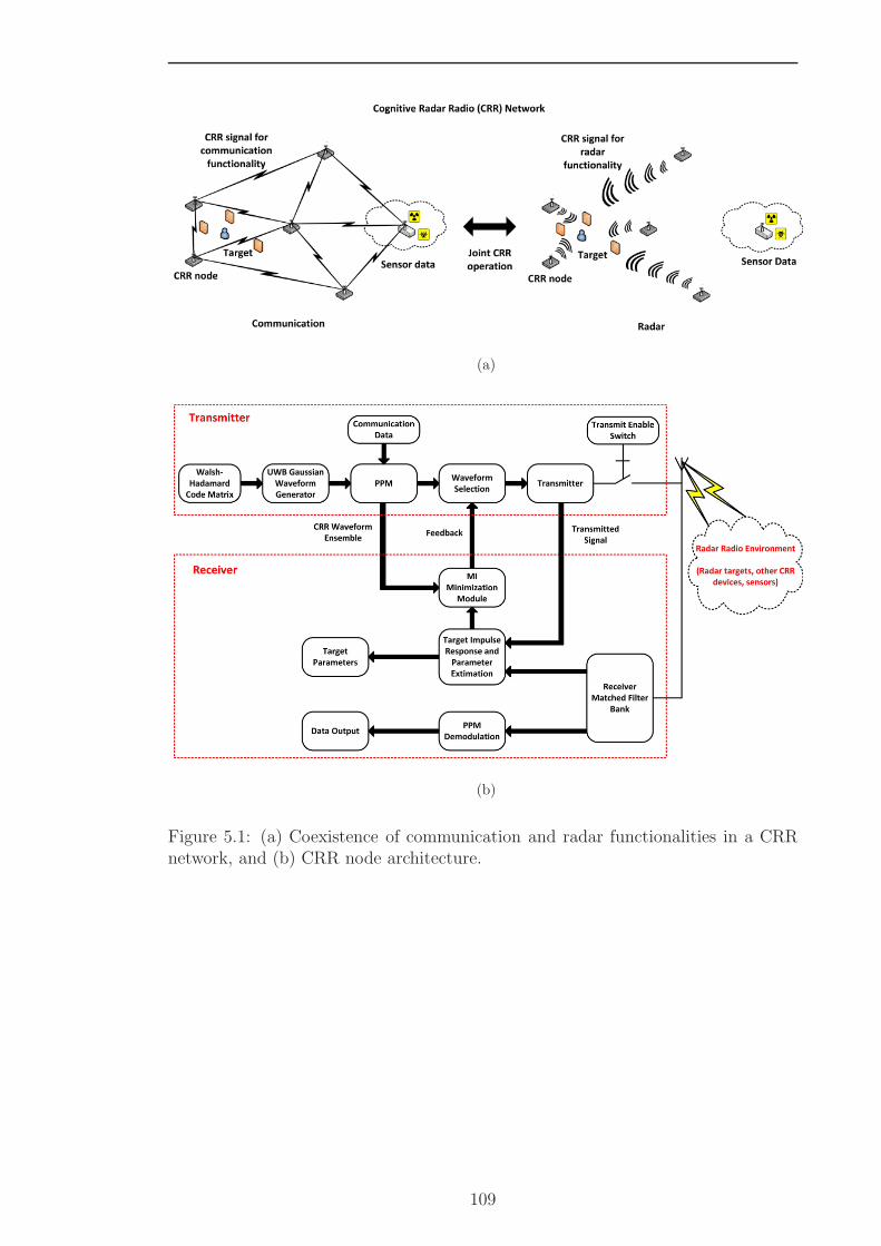
(a)

(b)

Figure 5.1: (a) Coexistence of communication and radar functionalities in a CRRnetwork, and (b) CRR node architecture.

109

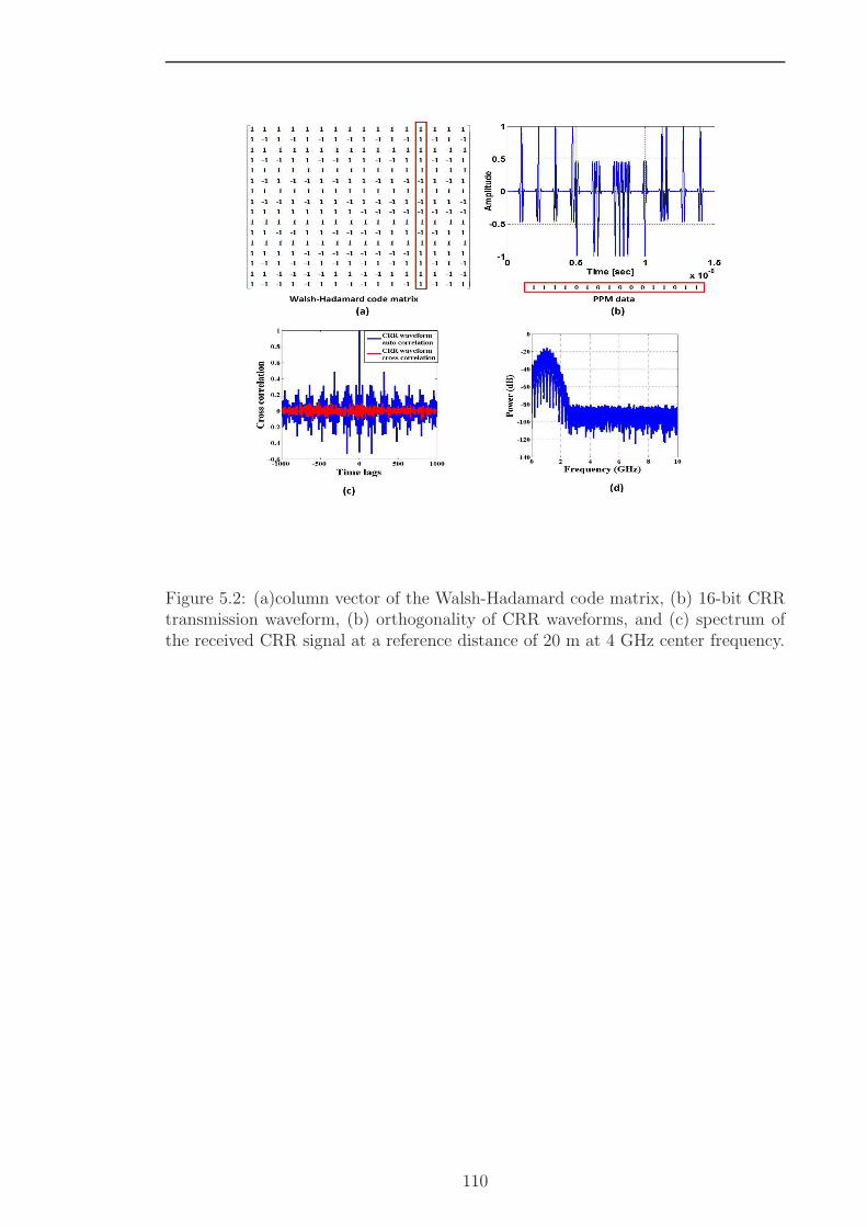
Figure 5.2: (a)column vector of the Walsh-Hadamard code matrix, (b) 16-bit CRRtransmission waveform, (b) orthogonality of CRR waveforms, and (c) spectrum ofthe received CRR signal at a reference distance of 20 m at 4 GHz center frequency.

110

Figure 5.3: (a) Static target and non-target (clutter) scatterers resolved after 10iterations of MI minimization at a CRR node, and (b) target and clutter returnsafter 10 iterations of MI minimization.

111

Figure 5.4: (a) Minimization of MI algorithm at different SNRs, (b) probabilityof target detection against SCNR for various iterations of the MI minimizationalgorithm, and (c) probability of detection for waveform selection based on MI min-imization and static waveform assignment.

112

Figure 5.5: (a) BER of different joint communication-radar waveform designs, and(b) throughput performance against distance from a particular CRR node.

113

Figure 5.6: (a) Target range profile for a target velocity = 3.5 m/s for 4 s timeduration after 10 iterations of MI minimization, and (b) target and clutter returnsafter 10 iterations of MI minimization.

114

Figure 5.7: (a) UWB channel model, (b) average ranging error based on TOAestimation in the multipath UWB channel, and (c) average ranging error againstPRI in the multipath UWB channel.

5.6 Chapter Summary

In this chapter, a joint communication-radar waveform design solution for the CRR

network is developed. As indicated by the simulation results, the CRR waveform

optimization approach promises better target impulse response extraction and range

resolution. From a communications perspective, the proposed CRR waveform de-

sign also promises high data rate performance over short ranges. The radar and

communication signals share the same spectral and temporal domains using the

current design strategy. This approach was based upon constant learning of the

target environment and adapting the transmission waveform characteristics to suit

the dynamic target scene. Such a cognitive approach ensures maximum information

extraction from the radar scene and better target discrimination capability. The

115

proposed unified system would constitute a unique cost-efficient platform for future

intelligent surveillance applications, for which both environment sensing along with

the allocation of ad hoc communication links are essential. Such systems can be used

in mission-critical and military applications for addressing the remote surveillance

and communication issues simultaneously. It is envisaged that the future personal

communication and tracking devices will have comprehensive radar-like function,

such as spectrum sensing and localization, in addition to multi-mode and multi-

band communication capability.

116

Chapter 6

Location Aware Spectrum and

Power Allocation Algorithm for

Cognitive Wireless Systems

In this chapter, a novel approach to spectrum and power allocation is proposed for

joint cognitive communication-radar networks, which aim at integrating cognitive

radio and cognitive radar paradigms to achieve intelligent utilization of spectrum

resources in wireless networks. The CRR nodes discussed in chapter 5 are mobile

radar units capable of extracting target parameters in the radar environment and are

able to simultaneously exchange communication data over the CRR network. The

communication functionality was an added feature to the CRR node design. On the

other hand, the CRR units, proposed in this chapter are wireless devices which have

the main purpose of exchanging data over the network. Although they will benefit

from the physical location information provided by the cognitive radar aspect of the

CRR design, exchange of data over the network is the primary function served by

the CRR nodes in the network. For example, the CRR network presented in chapter

5 could be applied to a battlefield scenario in which the soldiers could carry hand-

held wireless devices or CRR units, capable to track down a mobile target and at

the same time exchange vital radar scene information through the communication

link. Whereas in this chapter, the CRR nodes represent the wireless devices like

routers and hubs, which have a sole purpose of exchanging data over the network

and are empowered with location information on other devices and users through

the cognitive radar component in their design. Thus CRR nodes described in this

117

chapter are primarily radio units and the CRR nodes mentioned in chapter 5 are

mainly radar units.

This approach exploits the location information offered by cognitive radar com-

bined with spectrum sensing capability of cognitive radio to aid spectrum and power

allocation by minimizing harmful interference among neighboring devices. Such sys-

tems require both coexistence and sharing of perception of radio environment and

radar scene. To offer better spectrum resource utilization, entropy of the received

signal is employed in order to detect spectrum holes over the network topology. This

entropy-based technique also demonstrates superior performance as compared to the

conventional method based on energy detection. Simulation results indicate both

throughput improvement and interference reduction among neighboring devices.

After designing the approach to spectrum and power allocation for the CRR

network, the second aspect of this chapter is to investigate the inclusion of a cognitive

mechanism in predicting the spectral holes over the CRR network, by adopting a

HMM learning approach. Such a cognitive mechanism would enhance the overall

throughput of the entire network, since the wireless devices operating with the CRR

nodes would now be able to utilize the white spaces in the spectrum. To realize

opportunistic spectrum access, spectrum sensing is applied to detect the presence of

spectrum holes. If SUs randomly or sequentially sense the channels until a spectrum

hole is detected, significant amount of the scarce spectrum resource will be wasted,

since SUs transmit only after a decision has been made. On the other hand, with the

use of an intelligent predictive method, SUs can learn from the past activities of PUs

on each channel to predict the next channel state. By prioritizing the order in which

channels are sensed according to the channel availability likelihoods, the probability

that an SU gets a channel upon its first attempt significantly increases, thus reducing

the possible waste. Simulation results indicate improvement in throughput and

reduction in interference between neighboring wireless devices.

This inclusion of the cognitive mechanism for opportunistic spectrum access

over the CRR network facilitates the fusion of the cognitive radar and cognitive

radio paradigms. Such a fusion could achieve efficient power and spectrum resource

allocation in a wireless network.

118

6.1 Introduction

6.1.1 Location Aware Spectrum and Power Allocation

Dynamic spectrum access allows frequency bands to be assigned based on the needs

of radios without causing significant interference and degradation to the overall

throughput. The concept of system cognition proves to be an effective way for

intelligent spectrum management in wireless networks [87, 150]. The design and

implementation of cognitive radios that constantly adapt their operational modes

according to the changing radio environment are therefore necessary to utilize the

spectrum more efficiently [151]. In terms of cognitive radio, PUs of spectrum re-

sources are referred to as the authorized users of the radio channels and SUs compete

for the channels when PUs are inactive [87,150]. Hence, one of the most important

challenges of cognitive radio is spectrum hole detection, which is to acquire aware-

ness of the frequency usage and existence of PUs in neighboring bands. On the other

hand, when SUs are using the vacant channels, cognitive radio can also be aware of

initialization of any primary communication activities in their vicinity. The detec-

tion of PUs is very important, not only to prevent interference but also to detect

any opportunity of communication for SUs as shown in [87].

Location information of cognitive radio can prove to be beneficial in identifying

spectrum holes over the network, which can be used to assist in spectrum allocation

in order to avoid interference among users in close vicinity. This information can

be obtained from a dedicated cognitive radar network as discussed in [37, 88] and

chapters 3 and 4. This motivates the design of a novel CRR system presented in

the current work. Essentially, we combine the functionalities of cognitive radio and

cognitive radar to facilitate localization as well as intelligent spectrum and power

allocation. Specifically, in the CRR network studied in this chapter, radar targets

are primarily radio users, which results in coexistence of radio environment and

radar scene. Furthermore, the knowledge about the location and identification of

a specific radar target, which uses certain radio channels for communications, can

be fed into the cognitive radio network to assist in decision making about spectrum

assignment strategies. Similarly, the cognitive radio network can also localize and

identify the radio users by analyzing the received signal. This information can be

fed into the cognitive radar network to assist in radar waveform design and selection,

119

target state estimation, and power allocation [37, 88–90]. This leads to sharing of

perception of radio and radar scenes under surveillance.

Location information of CRUs can prove to be beneficial in identifying spectral

holes over the network. This location information can be used to assist spectrum

allocation in order to avoid interference between users in close vicinity. This would

allow the design and implementation of this innovative concept of CRR network for

various applications like remote detection, sensing, localization, tracking, monitor-

ing, transfer of information between wireless devices or between co-operative sensor

nodes.

IEEE 802.11b standard divides the spectrum into 14 overlapping, staggered chan-

nels whose center frequencies are 5 MHz apart. Given the separation between chan-

nels 1, 6, and 11, the signal on any channel could be sufficiently attenuated to

minimally interfere with a transmitter on any other channel located in the vicinity.

In this Chapter, we utilize these three channels for spectrum allocation between the

CRU.

The proposed CRR network is illustrated in Fig. 6.1. The system consists

of cognitive base stations (CBSs) at fixed locations and cognitive mobile stations

(CMSs) sharing 3 non-overlapping channels 1, 6 and 11 under IEEE 802.11b. A CBS

comprises a joint communication and radar platform (see e.g., the system concepts

proposed in [152,153]). On the other hand, a CMS is a radio user as well as a radar

target. For example, a RFID tag could be attached to a CMS for enhanced and rec-

ognizable RCS [37]. Subsequently, the radar components in CBSs transmit probing

waveforms, which are reflected by CMSs. The relevant information for positioning

such as RSS, TOA, and AOA is recorded at CBSs and forwarded to a cognitive

engine (CE) through wired links, which is the centralize decision-making entity as

shown in Fig. 6.1. The CE then works out the locations of CMSs by triangula-

tion [2]. It is worth emphasizing that, cognitive operations based on the experience

gained from the recognized radar-returns from CMSs could be implemented following

the cognitive radar concepts developed in [37, 88] and the previous chapters, which

include: (i) adaptive and continuous allocation of limited transmit power among

the activated CBSs; (ii) intelligent illumination of the environment through antenna

beamsteering at CBSs; and (iii) adjusting the set of activated CBSs to achieve the

optimized CMS detection and localization.

Subsequently, the spectrum holes are identified by using an information-theoretic

120

measure known as entropy of the received signal. Conventional spectrum sensing

methods include energy detection [154], matched filtering [155], and cyclostationarity-

based detection. Owing to its low computational complexity, the energy detection

algorithm is commonly used. This method requires knowledge of noise and signal

power. Nevertheless, the noise may not be stationary and its variance may not

be known a priori. On the other hand, matched filtering is the optimum method

for spectrum hole detection. However, it demands full knowledge of the signaling

features such as bandwidth, operating frequency, modulation type and order, pulse

shaping, etc. As a result, this method is not suitable for practical usage.

The entropy-based spectrum sensing can distinguish signals from noises be-

cause it is known that a stochastic signal with Gaussian pdf has the maximum

entropy [156]. This detection method has been proposed recently [157] and has

been proved to be intrinsically robust against noise uncertainty. The existence of

radio users over a channel is established when the entropy of the received signal

is smaller than a prescribed threshold. Each CMS constantly performs spectrum

sensing over the three available channels and notifies the availability of a particular

channel to the CE through the radio links with the CBSs as depicted in Fig. 6.1.

The CE then decides upon the optimal spectrum allocation strategy and determines

the corresponding operational parameters like transmission power for each CMS

by utilizing the location information in order to minimize interference and enhance

overall system throughput. Eventually, this enables an interference-suppressed sec-

ondary radio link between each pair of CMS and its neighboring SU as shown in

Fig. 6.1. For simplicity, we will assume that the SU is not a CMS (i.e., it is a radio

user but not a radar target).

The key contributions of this Chapter are:

1. Developing an algorithm based upon entropy of the received signal to detect

the radio user activity over a channel.

2. Fusing together cognitive radar and cognitive radio paradigms to achieve dy-

namic spectrum and power allocation over the wireless network.

3. Evaluation of network throughput and comparison of the proposed method

with conventional energy based detection.

4. Developing a cognitive spectrum access scheme for CRR units to facilitate

121

detection of spectral holes over the wireless network.

6.2 CRR Network Model

Figure 6.1: CRR network architecture.

We now present the analysis of the entropy-based spectrum sensing undertaken

by CMSs. This method establishes the presence or absence of a user over a radio

channel based upon hypothesis testing as follows

H0 : y(n) = η(n), n = 0, 1, ..., K − 1

H1 : y(n) = x(n) + η(n), n = 0, 1, ..., K − 1(6.1)

where H0 and H1 denote the absence and presence of the user, respectively. y(n)

is the received signal, x(n) indicates the transmitted signal from the user, η(n) is

the AWGN, and K denotes the number of samples over the observation period.

Therefore, the distribution of y(n) follows the Gaussian pdf as

H0 : y(n) ∼ N(0, σ2η)

H1 : y(n) ∼ N(µ, σ2x + σ2

η)(6.2)

122

where N(·, ·) denotes the normal distribution, σ2η is the noise variance, and µ and

σ2x are the mean and variance of the signal, respectively.

Applying discrete Fourier transform to (6.1) and (6.2), we obtain

H0 : Y(k) = η(k), k = 0, 1, ..., K − 1

H1 : Y(k) = X(k) + η(k), k = 0, 1, ..., K − 1(6.3)

where Y(k), X(k), and η(k) represent the complex vectors of received signal, trans-

mitted signal, and noise, respectively. Alternatively, Y(k) can also be written as

Y(k) =1

K

K−1∑

n=0

x(n) exp

(−j 2π

Kkn

)(6.4)

The detection strategy involves testing of the information entropy H(Y), which is

a measure of uncertainty associated with the random signal Y, defined as

H(Y) = −I∑

i=1

p(Yi) log2 p(Yi) (6.5)

In the preceding equation, I is the total number of countable states, often referred

to as the dimension of the probability space. p(Yi) denotes the probability of obser-

vation of a received signal level, Yi, such that∑I

i=1 p(Yi) = 1. We use the histogram

method for entropy estimation as suggested in [157]. Let o be the number of occur-

rences of received signal strength falling in the ith bin, Hence, p(Yi) ≈ oi/O with O

being the total number of occurrences. The bin width δ can be defined as

δ =Ymax − Ymin

I(6.6)

where Ymax and Ymin are the maximum and minimum values of the received signal

strength. Following (6.3) and (6.5), the estimated entropy (or the test statistic) is

given by

λ(Y) = H(Y) = −I∑

i=1

oiK

log2oiK

(6.7)

Subsequently, we utilize the above test statistic to evaluate the two hypotheses

123

for spectrum user detection

H0 : λ(Y) > λ0

H1 : λ(Y) ≤ λ0

(6.8)

where λ0 is the threshold determined by the probability of false alarm. The value

of λ will decrease according to the convex property of information entropy as the

channel changes its state from “free” to “busy”. In the next section we will describe

the algorithm for adapting transmission parameters of CMSs once spectral holes are

identified.

6.3 Spectrum and Power Allocation Algorithm

As described earlier, all the CMSs perform entropy-based spectrum sensing on the

three available radio channels and notify the CE about spectrum holes detected in

their neighboring regions. The CE takes into consideration the physical locations of

all the CMSs acquired through the radar units of the CBSs, and allots the available

frequencies with an intention of minimizing interference among neighboring CMSs.

It instructs each CMS to occupy a vacant channel and decides upon the transmission

power for each CMS with an objective of enhancing the overall system throughput.

The capacity of the radio link between two radio users can be expressed as [158,159]

C(ρ, η) = B log2

(1 +

ρ

1 + η

)(6.9)

where C(ρ, η) denotes the capacity of the radio link as a function of the SNR ρ, the

interference-to-noise ratio (INR) η, and the channel bandwidth B. Therefore, the

total capacity (or throughput) of the CRR network can be calculated as

C =

3∑

l=1

M∑

m=1

C

(αmm(l)Pm(l)

σ2η

,

∑n 6=m αmn(l)Pn(l)

σ2η

)

=3∑

l=1

M∑

m=1

C (ρm(l), ηm(l)) , n ∈ 1, 2, · · · ,M.(6.10)

In the preceding equation, l ∈ 1, 2, 3 is the index of the available channel, M is

the total number of point-to-point communication links using a particular channel,

αmm(l) represents the channel gain of link m using channel l, αmn(l) represents

124

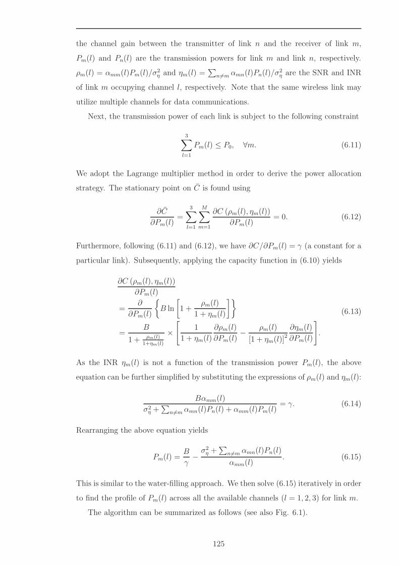
the channel gain between the transmitter of link n and the receiver of link m,

Pm(l) and Pn(l) are the transmission powers for link m and link n, respectively.

ρm(l) = αmm(l)Pm(l)/σ2η and ηm(l) =

∑n 6=m αmn(l)Pn(l)/σ

2η are the SNR and INR

of link m occupying channel l, respectively. Note that the same wireless link may

utilize multiple channels for data communications.

Next, the transmission power of each link is subject to the following constraint

3∑

l=1

Pm(l) ≤ P0, ∀m. (6.11)

We adopt the Lagrange multiplier method in order to derive the power allocation

strategy. The stationary point on C is found using

∂C

∂Pm(l)=

3∑

l=1

M∑

m=1

∂C (ρm(l), ηm(l))

∂Pm(l)= 0. (6.12)

Furthermore, following (6.11) and (6.12), we have ∂C/∂Pm(l) = γ (a constant for a

particular link). Subsequently, applying the capacity function in (6.10) yields

∂C (ρm(l), ηm(l))

∂Pm(l)

=∂

∂Pm(l)

B ln

[1 +

ρm(l)

1 + ηm(l)

]

=B

1 + ρm(l)1+ηm(l)

×[

1

1 + ηm(l)

∂ρm(l)

∂Pm(l)− ρm(l)

[1 + ηm(l)]2

∂ηm(l)

∂Pm(l)

].

(6.13)

As the INR ηm(l) is not a function of the transmission power Pm(l), the above

equation can be further simplified by substituting the expressions of ρm(l) and ηm(l):

Bαmm(l)

σ2η +

∑n 6=m αmn(l)Pn(l) + αmm(l)Pm(l)

= γ. (6.14)

Rearranging the above equation yields

Pm(l) =B

γ−σ2η +

∑n 6=m αmn(l)Pn(l)

αmm(l). (6.15)

This is similar to the water-filling approach. We then solve (6.15) iteratively in order

to find the profile of Pm(l) across all the available channels (l = 1, 2, 3) for link m.

The algorithm can be summarized as follows (see also Fig. 6.1).

125

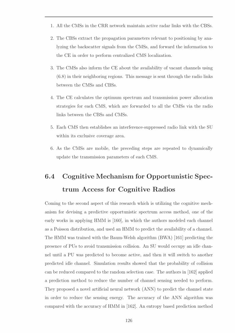
1. All the CMSs in the CRR network maintain active radar links with the CBSs.

2. The CBSs extract the propagation parameters relevant to positioning by ana-

lyzing the backscatter signals from the CMSs, and forward the information to

the CE in order to perform centralized CMS localization.

3. The CMSs also inform the CE about the availability of vacant channels using

(6.8) in their neighboring regions. This message is sent through the radio links

between the CMSs and CBSs.

4. The CE calculates the optimum spectrum and transmission power allocation

strategies for each CMS, which are forwarded to all the CMSs via the radio

links between the CBSs and CMSs.

5. Each CMS then establishes an interference-suppressed radio link with the SU

within its exclusive coverage area.

6. As the CMSs are mobile, the preceding steps are repeated to dynamically

update the transmission parameters of each CMS.

6.4 CognitiveMechanism for Opportunistic Spec-

trum Access for Cognitive Radios

Coming to the second aspect of this research which is utilizing the cognitive mech-

anism for devising a predictive opportunistic spectrum access method, one of the

early works in applying HMM is [160], in which the authors modeled each channel

as a Poisson distribution, and used an HMM to predict the availability of a channel.

The HMM was trained with the Baum-Welsh algorithm (BWA) [161] predicting the

presence of PUs to avoid transmission collision. An SU would occupy an idle chan-

nel until a PU was predicted to become active, and then it will switch to another

predicted idle channel. Simulation results showed that the probability of collision

can be reduced compared to the random selection case. The authors in [162] applied

a prediction method to reduce the number of channel sensing needed to perform.

They proposed a novel artificial neural network (ANN) to predict the channel state

in order to reduce the sensing energy. The accuracy of the ANN algorithm was

compared with the accuracy of HMM in [162]. An entropy based prediction method

126

was introduced in [163]. Authors looked for the correlated channels to optimize the

sensing strategy. In [164], the authors applied maximum likelihood to predict the

length of idle period of each channel. By selecting the channel with the longest

predicted idle time, they achieved a reduction in the number of channel switching

needed.

To realize opportunistic spectrum access, spectrum sensing is applied to detect

the presence of spectrum holes. If SUs randomly or sequentially sense the channels

until a spectrum hole is detected, significant amount of the scarce spectrum resource

will be wasted, since SUs transmit only after a decision has been made. On the other

hand, with the use of an intelligent predictive method, SUs can learn from the past

activities of each channel to predict the next channel state. By prioritizing the order

in which channels are sensed according to the channel availability likelihoods, the

probability that an SU gets a channel upon its first attempt significantly increases,

thus reducing the possible waste. This research introduces a learning-based HMM

to predict the channel activities. Simulation results show that the proposed HMM

can predict the channel activities with high accuracy after sufficient training. This

algorithm predicts the availability of the channels by only making use of the current

state of the spectrum. Furthermore, by incorporating the outcome of the actual

channel sense, the algorithm is able to make self-regulation before next decision, so

that errors will not propagate.

We present a novel HMM-based learning method to learn the behavior of PUs on

a channel and predict their activity in the next time slot. The number of states in

the proposed HMM is not fixed and grows as the training proceeds. We demonstrate

that this model can avoid propagation of error if an error occurs. The accuracy of

the proposed method is studied through simulation. We use a four-channel system

to illustrate the average number of channel sensing to be performed by an SU to

obtain a spectrum hole within a given probability of success.

6.4.1 Hidden Markov processes

In this study, the spectrum under consideration is divided into K channels and

each PU that transmits will occupy one of the channels. The presence of PUs on a

channel is represented with a “1” and the absence of PUs is shown with “0”. Some

simplifications are made in this learning model. We assume that channel sensings

127

are performed periodically (which is known as the time stamp) and the channel

sensing is ideal, i.e., the effects of noise, missed detection and false alarm errors

are negligible. An SU uses an HMM-based approach to learn about the PU usage

pattern of each channel through observing the outcomes of the channel sensing.

Using the trained HMM, SUs predict the availability of the channels for possible

usage in the next time slot through the algorithm to be introduced shortly.

A Hidden Markov Process is a doubly stochastic process with hidden states that

generate observations [118]. It is denoted mathematically as Xt, Yt; t ∈ N, wheret denotes the time stamp index which takes an integer number. X(t) is the N -state

hidden stochastic process, and X(t) ∈ Y where Y is the N possible states whose

transition probabilities are described by the N × N transition matrix A. Y (t) is

the stochastic process of the observations, and Y (t) ∈ O where O is the finite set of

possible observations withM possible outcomes. The distribution of the observation

outcomes at each state is described by the respective column vector of the N ×M

emission matrix B. The mathematical model that can generate a hidden Markov

process is called HMM. Similar to the HMM defined in chapter 4, this HMM model

can be described as λ = A,B, π. One of the main challenges in HMM is how to

adjust the model parameters (λ = A,B, π), to maximize Pr(O|λ), where Pr(·)represents probability.

In the following, we shall differentiate this approach with the conventional BWA-

based HMM approach.

6.4.2 Conventional BWA-based HMM

BWA [161] is the most commonly used method to estimate the maximum likelihood

of λ. To be able to predict, we have to gather some information from the channel

activities over the past time slots. Suppose that we observe the channel for T time

slots; having the HMM (λ), the channel state for the next time slot can be predicted

by the following rule

Y (t + 1) =

1 Pr(ζ, 1|λ) ≥ Pr(ζ, 0|λ)0 Pr(ζ, 1|λ) < Pr(ζ, 0|λ),

(6.16)

where ζ = Y (t− T + 1), ..., Y (t) denotes the past T observations.

In order to apply BWA, first the number of states (N) needs to be defined.

128

Since there is no information about the current state and previous states at the

time when parameters are estimated [161], hereafter we shall refer it as unknown-

state sequence HMM (USS-HMM). Since this approach needs to perform parameter

estimation in real-time for every prediction, the computation complexity is high,

as will be discussed later. Other challenges for this approach include defining the

optimum number of states (N) and the observation sequence length (T ) for an

accurate estimation.

6.4.3 Proposed HMM

Under the assumption that the statistics of the channel activities remain unchanged,

which means that the Doppler spread of the signal remains less than the signal

bandwidth, the prediction will be performed much faster through training. This

means that we consider a wide sense stationary channel activity instead of a time-

varying channel. The functional block diagram of the proposed method is shown

in Fig. 6.2. As shown in the figure, the HMM is trained with a certain number of

observations until a satisfactory convergence of the HMM parameters is achieved.

After training, the HMM predictor only needs the current observation to predict

the next channel state. This is unlike USS-HMM, where there is a need to use a

sequence of observations to iteratively compute every prediction. In this algorithm,

re-train is needed only if the channel statistics have changed. In order to prevent the

propagation of the error in predictions, the HMM model is retrained if the channel

statistics change.

The channel state at the next time slot will be predicted by

Y (t+ 1) =

1 Pr(S(t), 1|λ) ≥ Pr(S(t), 0|λ)0 Pr(S(t), 1|λ) < Pr(S(t), 0|λ),

(6.17)

where S(t) is the HMM state at time slot t. In this approach, since the proposed

HMM knows the state sequence as well as the observation sequence, to distinguish

from USS-HMM, the proposed HMM is referred to as the known-state sequence

HMM (KSS-HMM).

We now provide more details about the HMM model as shown in Fig. 6.3. The

number of states (i.e. N) in this model grows dynamically as learning proceeds.

zero represents the initial state. The negative and positive states represent unused

129

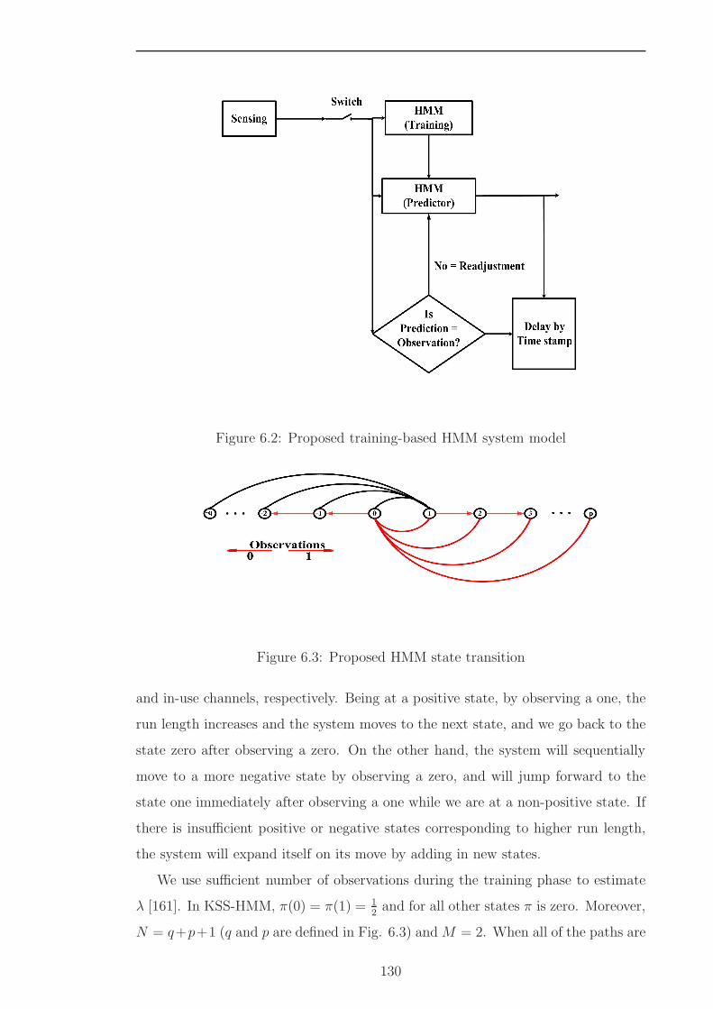
Figure 6.2: Proposed training-based HMM system model

Figure 6.3: Proposed HMM state transition

and in-use channels, respectively. Being at a positive state, by observing a one, the

run length increases and the system moves to the next state, and we go back to the

state zero after observing a zero. On the other hand, the system will sequentially

move to a more negative state by observing a zero, and will jump forward to the

state one immediately after observing a one while we are at a non-positive state. If

there is insufficient positive or negative states corresponding to higher run length,

the system will expand itself on its move by adding in new states.

We use sufficient number of observations during the training phase to estimate

λ [161]. In KSS-HMM, π(0) = π(1) = 12and for all other states π is zero. Moreover,

N = q+p+1 (q and p are defined in Fig. 6.3) andM = 2. When all of the paths are

130

known, then it is possible to count the number of times each particular transition or

output observation is applied in a set of training data. It has been proven in [161]

that counting functions, say Φmn(x(t)) for the state transitions and Φkn(y(t)) for

the output observations provide the maximum likelihood estimates for the desired

model parameters, such that

amn =Φmn(x(t))∑

n

Φmn(x(t)), (6.18)

bkn =Φkn(y(t))∑

n

Φkn(y(t)). (6.19)

Φmn(x(t)) represent the number of state transitions from state m to state n and

Φkn(y(t)) represents the number of k observations while in state n. Thus amn and

bkn represent the relative frequency of state and observation instances as mentioned

in [118]. The basis of the proposed HMM is therefore to account the probabilities

of occurrence of different run lengths of ones (or zeros). Clearly, the number of

states (N) depends on how long the algorithm is trained, and hence it also affects

the accuracy of the training. Although a disadvantage of the algorithm is that we

have to deal with a situation where the number of states dynamically grows during

the training, there is a nice property about A and B in this model. Since the HMM

adopted in the algorithm has only two possible transitions from one state, therefore

the transition matrix A, is a sparse matrix. It is not difficult to figure out that the

non-zero elements in A is actually identical to the elements in the emission matrix.

In the following, we shall see that this simplifies the prediction process and enables

a corrective action to be taken if a prediction is in error.

The transition probability between any two states is denoted by

aij = Pr(x(t) = si|x(t− 1) = sj), (6.20)

where si and sj are the states at time t and t− 1, respectively, and aij denotes the

transition probability presented in the (i, j) element of the matrix A.

During the learning or training process, the transition and emission probability

over T observations can be easily calculated by (6.18) and (6.19). As there are only

two possible observation states, HMM is designed in a way that only two states

131

are reachable from the current state. Moreover the probability of transition from

current state to either of the two states is equal to the probability of observing either

a zero or a one. Thus having the emission matrix (B), means having the probability

of next state as well as the distribution of observations.

b1,i = ai,i+1, b0,i = ai,0 i > 0

b0,i = ai,i−1, b1,i = ai,1 i ≤ 0(6.21)

This property makes the states sequence trackable. With this property, the

proposed method is not required to compute the maximum likelihood over a long

sequence of observations for each prediction. Retraining the KSS-HMM is only

needed when the behavior of PUs on the channel is changing.

A minimum separation factor (0 ≤ δ < 1) can be added to the decision criterion,

so it will look like:

Pr(S(t), 0|λ)− Pr(S(t), 1|λ) > δ. (6.22)

The purpose of prediction is to prioritize which channel to be sensed in the next

time instant. If (6.22) is satisfied, SU will sense the channel and transmit over the

channel only if the prediction is correct. On the other hand, if (6.22) is not satisfied,

SU will decide that the channel is occupied on t+1. It is obvious that if δ = 0, (6.22)

is equivalent to (6.17). In case of an inaccurate prediction, the system will notice

the prediction error after the sensing. Since S(t + 1) only depends on observation

outcome rather than predicted result, the system will move to the correct state and

errors will not propagate.

6.5 Simulation Results

6.5.1 Simulation Results for Location Aware Spectrum and

Power Allocation

For the purpose of simulation, we assume a square grid of 10×10 CMSs sharing the

three available channels under IEEE 802.11b. Fig. 6.4 indicates the initial random

channel assignment over the CMSs. Each CMS occupies a square footprint and

communicates with an SU within this exclusive coverage area. Each color (blue,

red, or yellow) represents one of the three available channels (1, 6 and 11). The

132

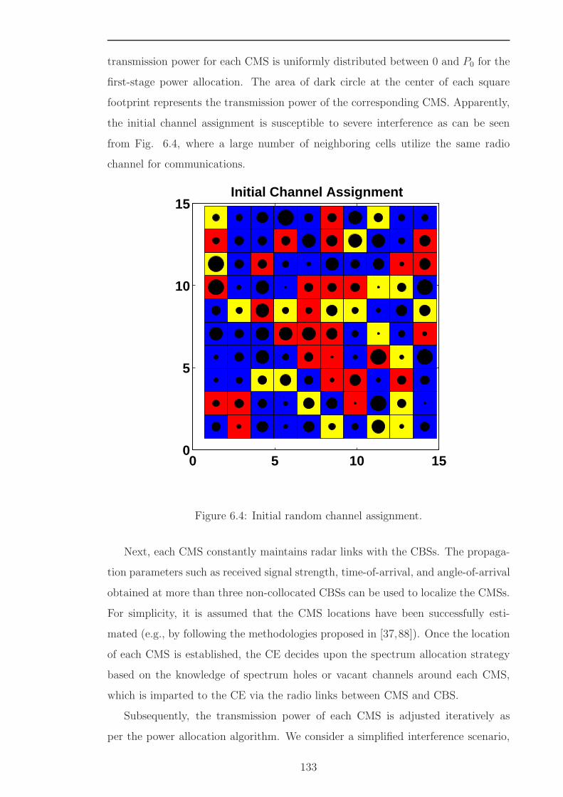
transmission power for each CMS is uniformly distributed between 0 and P0 for the

first-stage power allocation. The area of dark circle at the center of each square

footprint represents the transmission power of the corresponding CMS. Apparently,

the initial channel assignment is susceptible to severe interference as can be seen

from Fig. 6.4, where a large number of neighboring cells utilize the same radio

channel for communications.

0 5 10 150

5

10

15Initial Channel Assignment

Figure 6.4: Initial random channel assignment.

Next, each CMS constantly maintains radar links with the CBSs. The propaga-

tion parameters such as received signal strength, time-of-arrival, and angle-of-arrival

obtained at more than three non-collocated CBSs can be used to localize the CMSs.

For simplicity, it is assumed that the CMS locations have been successfully esti-

mated (e.g., by following the methodologies proposed in [37,88]). Once the location

of each CMS is established, the CE decides upon the spectrum allocation strategy

based on the knowledge of spectrum holes or vacant channels around each CMS,

which is imparted to the CE via the radio links between CMS and CBS.

Subsequently, the transmission power of each CMS is adjusted iteratively as

per the power allocation algorithm. We consider a simplified interference scenario,

133

0 5 10 150

5

10

15Final Channel Assignment

Figure 6.5: Final location-aware channel assignment.

0 10 20 30 40 500.4

0.5

0.6

0.7

0.8

0.9

1

Iteration

Th

rou

gh

pu

t

SNR=20dBSNR=−5dBSNR=−10dBSNR=−20dB

Figure 6.6: CRR network throughput.

134

−25 −20 −15 −100

0.2

0.4

0.6

0.8

1

SNR (dB)

Pro

ba

bility o

f d

ete

ctio

n

Entropy−based detector

Energy−based detector

Figure 6.7: Performance of spectrum user detection.

where the two channel gains αmm and αmn in (6.10) are assumed to be two fixed

constants. Furthermore, only the first-tier interferers (i.e., for each CMS under

consideration, its immediate 8 neighboring cells) are taken into account for power

allocation using (6.15). The main intention of this spectrum and power allocation

algorithm is to avoid clustering of CMSs using the same channel, and to distribute

transmission power according to the water-filling approach in order to enhance the

overall throughput. Fig. 6.5 indicates the final channel assignment. In this case, we

observe lower number of neighboring CMSs sharing the same channel. This indicates

reduction of interference among CMSs.

Fig. 6.6 illustrates the throughput of the overall system. Each characteristics

curve in this plot represents a throughput at a particular value of SNR. It can be

seen that the throughput converges after a certain number of iterations for each

SNR. In general, faster convergence is achieved for higher SNRs. Nevertheless, in

the case of very low SNR (SNR = −20 dB), more iterations fail to result in improved

throughput.

Finally, Fig. 6.7 demonstrates the performance of the entropy-based detector

as compared against the energy-based detector. These results have been gener-

ated by averaging over 100 simulations at different SNRs. The probability of false

alarm has been fixed at 0.15 for evaluating the value of the threshold λ0 in (6.8).

As discussed previously, the entropy-based detector does not require any previous

knowledge about transmission parameters of the signal or noise characteristics. It is

135

0 200 400 600 800 1000 1200 1400 1600 1800 200076

78

80

82

84

86

88

90

92

94

Training sequence Length

Pred

ictio

n Ac

cura

cy (p

erce

nts)

Arrival mean=10Arrival mean=12Arrival mean=14Arrival mean=16Arrival mean=18Arrival mean=20Arrival mean=22

Figure 6.8: KSS-HMM prediction accuracy on test data set

also quite robust and insensitive to noise uncertainty. Thus its performance is supe-

rior as compared to the energy-based detection in terms of probability of spectrum

user detection even at lower SNRs as can be seen from Fig. 6.7.

6.5.2 Simulation Results on Cognitive Mechanism for Op-

portunistic Spectrum Access

This section presents some simulation results of KSS-HMM and USS-HMM. To

evaluate the prediction accuracy, the statistics of PU activities on each channel are

assumed to remain unchanged over the simulation period. It is assumed that the

average traffic intensity (γ) calculated by (6.23) is equal to 0.5, which means that

the mean of ON and OFF periods are considered equal.

γ =Mean ON time

Mean Arrival Time(6.23)

Moreover, we set δ = 0 for the current simulations. Channel activities are generated

as training and test datasets for various mean arrival times, from 10 to 20 time

slots between arrivals. Fig. 6.8 shows the KSS-HMM prediction accuracy for dif-

ferent mean arrival (poisson) values. As expected the prediction accuracy improves

by increasing the length of the training sequence. Clearly using 1000 samples is

sufficiently good to generate stable training results.

In Fig. 6.9, the total error probability, and error probabilities in prediction of the

136

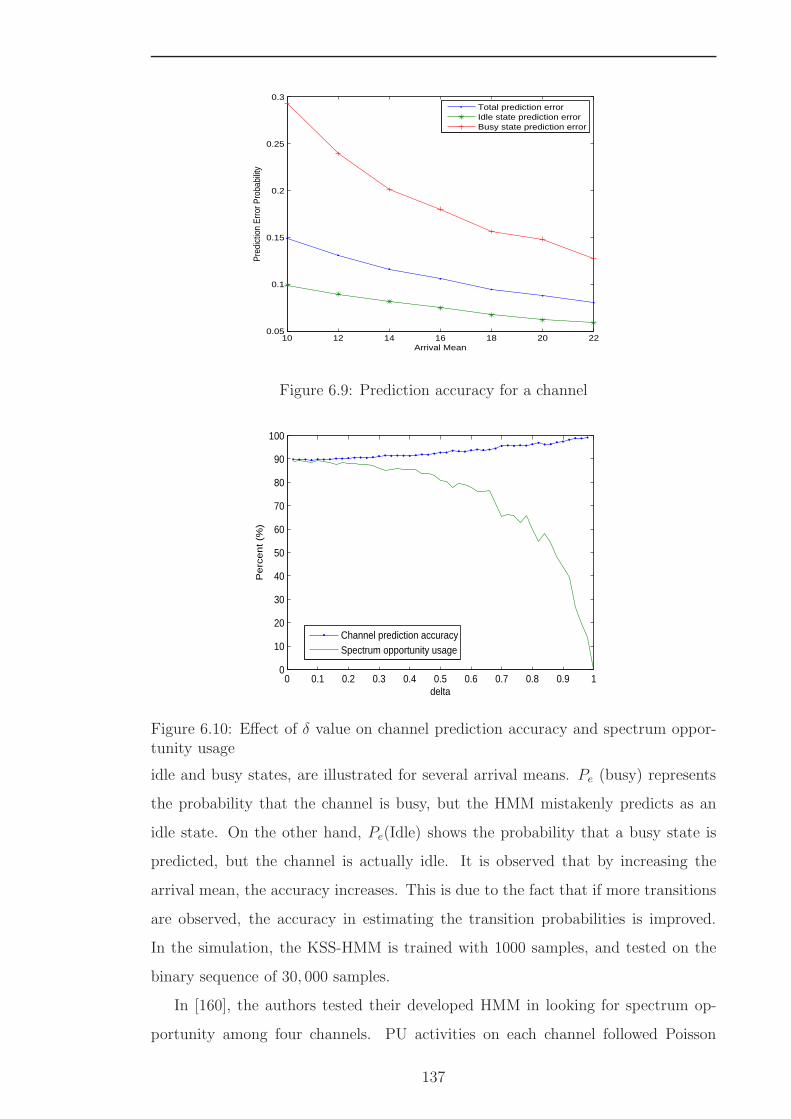
10 12 14 16 18 20 220.05

0.1

0.15

0.2

0.25

0.3

Arrival Mean

Pred

ictio

n Er

ror P

roba

bilit

y

Total prediction errorIdle state prediction errorBusy state prediction error

Figure 6.9: Prediction accuracy for a channel

0 0.1 0.2 0.3 0.4 0.5 0.6 0.7 0.8 0.9 10

10

20

30

40

50

60

70

80

90

100

delta

Perc

ent (%

)

Channel prediction accuracySpectrum opportunity usage

Figure 6.10: Effect of δ value on channel prediction accuracy and spectrum oppor-tunity usage

idle and busy states, are illustrated for several arrival means. Pe (busy) represents

the probability that the channel is busy, but the HMM mistakenly predicts as an

idle state. On the other hand, Pe(Idle) shows the probability that a busy state is

predicted, but the channel is actually idle. It is observed that by increasing the

arrival mean, the accuracy increases. This is due to the fact that if more transitions

are observed, the accuracy in estimating the transition probabilities is improved.

In the simulation, the KSS-HMM is trained with 1000 samples, and tested on the

binary sequence of 30, 000 samples.

In [160], the authors tested their developed HMM in looking for spectrum op-

portunity among four channels. PU activities on each channel followed Poisson

137

Table 6.1: ON/OFF period means for different channels

Channel 1 2 3 4ON period mean 5 7 4 8OFF period mean 5 7 4 8

Table 6.2: Comparison of KSS-HMM and USS-HMM prediction accuracy

HMM typeArrival mean

10 12 14 16 18 20 22KSS-HMM 0.8388 0.8524 0.8830 0.8936 0.9016 0.9088 0.9192USS-HMM 0.8478 0.8588 0.8858 0.8918 0.9076 0.9124 0.9184

distribution with equal mean for the ON and OFF durations. A similar approach

is used to test the performance of the proposed HMM. In this scenario, we trained

a KSS-HMM for each channel with 1000 samples and tested for 30, 000 samples.

The effect of different values of δ on the channel prediction accuracy and the per-

centage that spectrum holes are properly made use of, are shown in Fig. 6.10. In

this simulation, a channel prediction is said to be accurate if we successfully predict

an empty channel for transmission among the four channels. As can be seen, the

increase of δ leads to increase in the accuracy, but reduces the number of oppor-

tunities that are caught by the SU. Another issue which must be discussed is the

acceptable accuracy of predicting an idle channel in a time slot. Table 6.1 shows the

mean of Poisson distribution for both ON and OFF periods. Fig. 6.11 compares

the learning based and random channel selection approaches for the aforementioned

scenario. As it could be expected the random selection succeeds only about 50% of

time, while the learning based approach caches the available channel on its first at-

tempt in over 90% of its attempts. In learning based approach, only less than 0.02%

of attempts were not successful until checking the last channel, while about 7% of

random channel selection attempts were unsuccessful till the last check. Compared

to KSS-HMM, the complexity of USS-HMM is much higher. The training complex-

ity for KSS-HMM is 2(T +1)×N , where T is the training sequence length and N is

the number of states. Furthermore, KSS-HMM training is done only once and after

that whenever it is required. Therefore the actual training calculations required for

each KSS-HMM prediction is (2(T +1)×N)/τ , where τ is the number of predictions

made without the need for retraining. Moreover, each KSS-HMM decision lays only

on a hyperplane test. On the other hand, USS-HMM has N2T calculations after the

138

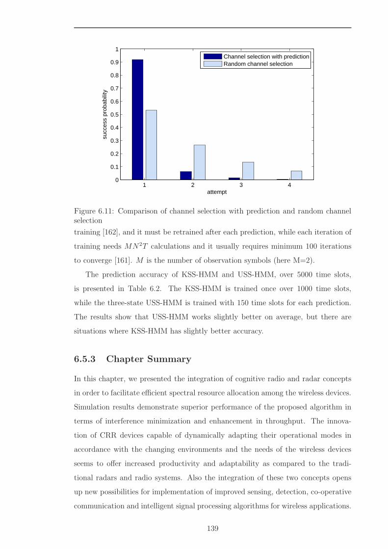
1 2 3 40

0.1

0.2

0.3

0.4

0.5

0.6

0.7

0.8

0.9

1

attempt

succ

ess

prob

abili

ty

Channel selection with predictionRandom channel selection

Figure 6.11: Comparison of channel selection with prediction and random channelselection

training [162], and it must be retrained after each prediction, while each iteration of

training needs MN2T calculations and it usually requires minimum 100 iterations

to converge [161]. M is the number of observation symbols (here M=2).

The prediction accuracy of KSS-HMM and USS-HMM, over 5000 time slots,

is presented in Table 6.2. The KSS-HMM is trained once over 1000 time slots,

while the three-state USS-HMM is trained with 150 time slots for each prediction.

The results show that USS-HMM works slightly better on average, but there are

situations where KSS-HMM has slightly better accuracy.

6.5.3 Chapter Summary

In this chapter, we presented the integration of cognitive radio and radar concepts

in order to facilitate efficient spectral resource allocation among the wireless devices.

Simulation results demonstrate superior performance of the proposed algorithm in

terms of interference minimization and enhancement in throughput. The innova-

tion of CRR devices capable of dynamically adapting their operational modes in

accordance with the changing environments and the needs of the wireless devices

seems to offer increased productivity and adaptability as compared to the tradi-

tional radars and radio systems. Also the integration of these two concepts opens

up new possibilities for implementation of improved sensing, detection, co-operative

communication and intelligent signal processing algorithms for wireless applications.

139

The second part of this chapter focused on HMM-based cognitive algorithm which

can be used for channel activity prediction of the CRR devices. As investigated in

the second part, the CRR nodes can detect spectral holes over the network through

the predictive opportunistic spectrum access algorithm. This enhances the overall

throughput of the CRR network. The algorithm is simple in principle and predic-

tions can be made without the need to perform sophisticated optimization. Using

the fact that channel sensing is still necessary before SU transmission even predic-

tion is made, the algorithm can make use of this observation later to self-correct any

prediction error occurs. The performance of the prediction algorithm is examined

through simulation and compared with the random channel access method. This

study also has shown that the proposed HMM model can achieve nearly the same

performance as the conventional USS-HMM model in the channel selection problem.

140

Chapter 7

Conclusion and Future Work

In this thesis, we have investigated various cognitive architectures for designing

radar systems. The striking difference between traditional and cognitive radar sys-

tem designs is the ability of the radar receiver to offer a cognitive feedback to the

transmitter, which enables it to implement intelligent illumination of the radar scene.

The major advantage of such a system design is the ability of the radar system to

adapt to the dynamically varying radar environment. The radar system can adapt

its operational parameters by constantly interacting with the radar environment and

gaining updated target parameter information. Such an architecture enables the in-

telligent target illumination strategies like adaptive waveform design and intelligent

selection of radar units for a network scenario.

The motivation behind this research was to explore various cognitive mecha-

nisms, which would enable the design of intelligent radar systems capable of adapting

its operational modes in accordance with target dynamics. In Chapter 3, a cogni-

tive waveform optimization approach was investigated for MIMO radar systems. In

this approach we adopted a two-step procedure based on MI optimization to design

the MIMO radar waveforms. The objective behind such a waveform optimization

approach was to gain the information on target parameters through the proposed

iterative optimization approach. The first of this two step procedure comprised of

waveform design based on maximization of MI between estimated target impulse

and received radar signal with an objective to “match” the transmitted waveform

with the target impulse response. This step was based on recent works on infor-

mation theory based waveform design methods. The second step was developed in

order to minimize the MI between the successive received radar echoes in order to

141

ensure that the subsequent received signals remain statistically independent over the

temporal domain in a bid to gain updated target impulse response estimate. Both

these approaches work in tandem to produce significant performance gains in terms

of detection probability and target parameter extraction capability of the radar sys-

tem. In Chapter 4, we investigated the HMM based tracking application wherein the

HMM based model estimated the target dynamics by learning the trajectory. This

tracking approach was utilized to predict the nearest set of radar units in the vicinity

of the target in the next time instant. This enabled significant power savings and

also made possible the realization of the track-before-detect mechanism. As demon-

strated by the simulation results the tracking capability of the proposed approach

was comparable to the standard benchmark methods for target tracking even though

only a limited set of radar units were required to perform the cognitive detection

of the target. This approach was also found to be suitable to track fast moving

targets since the HMM tracking model allowed continual learning on the target dy-

namics. The algorithm was not only found to have comparable execution times with

the standard benchmark methods but also provided better localization performance

with respect to the step size of the target. In Chapter 5, we investigated the joint

communication-radar waveform design method based on cognitive principles. This

approach allowed the distinct wireless nodes to exchange radar scene information

between themselves using the same waveform used for performing radar operations.

The motivation of this joint cognitive radar radio (CRR) waveform design method

was in mission critical and military applications. In such applications, there is a

need to exchange communications data as well as perform radar operations using a

smart waveform design approach. Simulation results have demonstrated that perfor-

mance of such a waveform design in terms of BER and throughput is comparable to

the joint communication-radar design mechanisms mentioned in the literature. The

radar performance in terms of target detection and parameter extraction is greatly

enhanced by utilizing cognitive approach for waveform selection. In Chapter 5 the

CRR nodes are mobile radar units with a communication capability. Whereas in

Chapter 6 the CRR units are radio users equipped with location information of other

neighboring CRR units provided through a radar module. The possible integration

of cognitive radio and cognitive radar paradigms is investigated in this chapter. By

achieving such a fusion of paradigms efficient resource utilization in terms of trans-

mission power and spectral resources could be achieved over a wireless network.

142

This work focused on the location aware spectrum and power allocation for wireless

network. The location information on wireless devices gained through utilization of

cognitive radar units was coupled with the spectrum sensing ability of the cognitive

radio mechanism to realize this intelligent resource allocation algorithm. In this

chapter we also investigated the cognitive opportunistic spectrum access mechanism

in order to efficiently sense the wireless environment to gain information over possi-

ble spectral holes. This information could be exploited by SUs for communication

thus enhancing the overall throughput of the wireless network.

Future works in this research field could involve extending this idea of cognitive

radar network system, which incorporates several radars working together in a co-

operative manner with the goal of realizing a remote-sensing capability far in excess

of what the radar components are capable of achieving individually. In the extended

target recognition application, the cognitive radar network can provide more robust

detection performance, more accurate position estimation, and more reliable target

aspect angle for each radar. By utilizing a cognitive architecture for MIMO radars,

the issue of target-aspect sensitivity can be solved even for maneuvering targets by

adapting the radar transmission parameters like the waveform shape, power and

frequency. In this way, cognitive mechanisms could be applied for the development

of more complex radar architectures like on-board radars in remote air-surveillance.

Cognitive radar system design could be extended to implement waveform design so-

lutions for hostile indoor and outdoor channel environments where the radar chan-

nels are highly time variant and the target responses are suppressed by strong clutter

or non-target sources in applications like tracking movement of human subjects in an

indoor environment. Cognitive radars could also be designed for bio-medical appli-

cations like synthesis of body area networks for remotely observing and monitoring

the physiological and physical conditions of patients.

Another interesting avenue for research is the fusion of cognitive radar and cog-

nitive radio paradigms which can result in the development of cognitive dynamic

systems for wireless applications. Both of these models strive to impart intelligence

to traditional wireless systems which utilize a static framework for resource manage-

ment and hence are not able to cope up with the ever increasing demands of wireless

devices being deployed. From a technological perspective, the innovation of CRR

devices presented in this thesis, which are capable of dynamically adapting their op-

erational modes in accordance with the changing environments and the needs of the

143

wireless devices, seems to offer increased productivity and adaptability as compared

to the traditional radars and radio systems. The CRR system design and results

presented in this thesis could be extended to flexible mobile sensor network appli-

cations such as new ambient intelligence applications in environment monitoring,

robotics, intelligent cars and traffic systems, smart homes, health monitoring and

industrial automation. The results presented in this thesis open up new possibilities

for implementation of improved sensing, decentralized detection, development of co-

operative radar systems and intelligent signal processing algorithms for wireless and

radar applications.

144

References

[1] B. R. Mahafza and A. Z. Elsherbeni, Matlab Simulations for Radar Systems

Design. 1st Ed., CRC Press,Chapman and Hall, 2005.

[2] M. L. Skolnik, Introduction to Radar systems, 3rd Ed. McGraw-Hill Publica-

tions, New York, 2001.

[3] M. Bell, “Information theory and radar waveform design,” IEEE Trans. In-

form. Theory, vol. 39, no. 12, pp. 1578–1597, 1993.

[4] J. R. Guerci, Space-Time Adaptive Processing. Artech House, Norwood, MA,

2003.

[5] J. Guerci and E. Baranoski, “Knowledge-aided adaptive radar at DARPA: an

overview,” IEEE Signal Process. Mag., vol. 23, no. 1, pp. 41–50, Jan. 2006.

[6] P. Stoica, J. Li, X. Zhu, and J. Guerci, “On using a priori knowledge in space-

time adaptive processing,” IEEE Trans. Signal Process., vol. 56, no. 6, pp.

2598–2602, June 2008.

[7] R. Romero and N. Goodman, “Information-theoretic matched waveform in

signal dependent interference,” in Proc. IEEE Radar Conference, May 2008,

pp. 1–6.

[8] D. Garren, M. Osborn, A. Odom, J. Goldstein, S. Pillai, and J. Guerci, “En-

hanced target detection and identification via optimised radar transmission

pulse shape,” IEE Proceedings Radar, Sonar and Navigation, vol. 148, no. 3,

pp. 130–138, June 2001.

[9] N. Goodman, P. Venkata, and M. Neifeld, “Adaptive waveform design and

sequential hypothesis testing for target recognition with active sensors,” IEEE

J. Sel. Topics Signal Process., vol. 1, no. 1, pp. 105–113, June 2007.

145

[10] Y. Wei, H. Meng, Y. Liu, and X. Wang, “Radar phase-coded waveform design

for extended target recognition under detection constraints,” in Proc. IEEE

Radar Conference (RADAR), May 2011, pp. 1074–1079.

[11] E. Fishler, A. Haimovich, R. Blum, D. Chizhik, L. Cimini, and R. Valen-

zuela, “MIMO radar: an idea whose time has come,” in Proc. the IEEE Radar

Conference., April 2004, pp. 71–78.

[12] D. Rabideau and P. Parker, “Ubiquitous MIMO multifunction digital array

radar,” in Proc. Thirty-Seventh Asilomar Conference on Signals, Systems and

Computers., vol. 1, Nov. 2003, pp. 1057–1064.

[13] J. Zhang, H. Wang, and X. Zhu, “Adaptive waveform design for separated

transmit/receive ULA-MIMO radar,” IEEE Trans. Signal Process., vol. 58,

no. 9, pp. 4936–4942, Sept. 2010.

[14] T. Barnard and D. Weiner, “Non-Gaussian clutter modeling with generalized

spherically invariant random vectors,” IEEE Transactions on Signal Process-

ing, vol. 44, no. 10, pp. 2384–2390, Oct 1996.

[15] L. Brennan and L. Reed, “Theory of Adaptive Radar,” IEEE Transactions

on Aerospace and Electronic Systems, vol. AES-9, no. 2, pp. 237–252, March

1973.

[16] D. Zhang, F. Xia, Z. Yang, L. Yao, and W. Zhao, “Localization technologies

for indoor human tracking,” in Proc. 5th International Conference on Future

Information Technology (FutureTech), May 2010, pp. 1–6.

[17] P. Dutta, A. Arora, and S. Bibyk, “Towards radar-enabled sensor networks,” in

Proc. The Fifth International Conference on Information Processing in Sensor

Networks (IPSN), 2006, pp. 467–474.

[18] R. Thoma, O. Hirsch, J. Sachs, and R. Zetik, “UWB sensor networks for

position location and imaging of objects and environments,” in Proc. The

Second European Conference on Antennas and Propagation (EuCAP), Nov.

2007, pp. 1–9.

[19] J. Choliz, M. Eguizabal, A. Hernandez-Solana, and A. Valdovinos, “Compar-

ison of algorithms for UWB indoor location and tracking systems,” in Proc.

146

IEEE 73rd Vehicular Technology Conference (VTC Spring), May 2011, pp.

1–5.

[20] S. Gezici, Z. Tian, G. Giannakis, H. Kobayashi, A. Molisch, H. Poor, and

Z. Sahinoglu, “Localization via ultra-wideband radios: a look at positioning

aspects for future sensor networks,” IEEE Signal Process. Mag., vol. 22, no. 4,

pp. 70–84, July 2005.

[21] F. Cao and D. Wang, “Accurate wireless location and tracking technique for

indoor UWB non-linear/non-gaussian systems,” in Proc. Third International

Conference on Communications and Mobile Computing (CMC), April 2011,

pp. 449–452.

[22] M. Najar, J. Huerta, J. Vidal, and J. Castro, “Mobile location with bias track-

ing in non-line-of-sight,” in Proc. IEEE International Conference on Acoustics,

Speech, and Signal Process. (ICASSP), vol. 3, May 2004.

[23] D. Garmatyuk, J. Schuerger, Y. Morton, K. Binns, M. Durbin, and J. Kimani,

“Feasibility study of a multi-carrier dual-use imaging radar and communica-

tion system,” in Proc. European Radar Conference (EuRAD)., Oct. 2007, pp.

194–197.

[24] S. C. Surender and R. M. Narayanan, “UWB noise-OFDM netted radar: Phys-

ical layer design and analysis,” IEEE Trans. Aerosp. Electron. Syst., vol. 47,

no. 2, pp. 1380–1400, Apr. 2011.

[25] D. Garmatyuk, J. Schuerger, Y. Morton, K. Binns, M. Durbin, and J. Kimani,

“Feasibility study of a multi-carrier dual-use imaging radar and communica-

tion system,” Proc. European Radar Conference (EuRAD), pp. 194–197, 2007.

[26] D. Garmatyuk and J. Schuerger, “Conceptual design of a dual-use

radar/communication system based on OFDM,” in Proc. IEEE Military Com-

munications Conference (MILCOM), Nov. 2008, pp. 1–7.

[27] D. Garmatyuk, J. Schuerger, and K. Kauffman, “Multifunctional software-

defined radar sensor and data communication system,” IEEE Sensors Journal,

vol. 11, no. 1, pp. 99–106, Jan. 2011.

147

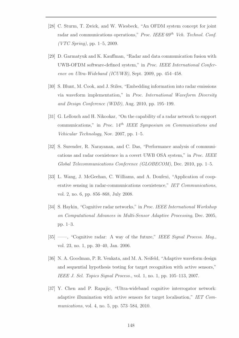
[28] C. Sturm, T. Zwick, and W. Wiesbeck, “An OFDM system concept for joint

radar and communications operations,” Proc. IEEE 69th Veh. Technol. Conf.

(VTC Spring), pp. 1–5, 2009.

[29] D. Garmatyuk and K. Kauffman, “Radar and data communication fusion with

UWB-OFDM software-defined system,” in Proc. IEEE International Confer-

ence on Ultra-Wideband (ICUWB), Sept. 2009, pp. 454–458.

[30] S. Blunt, M. Cook, and J. Stiles, “Embedding information into radar emissions

via waveform implementation,” in Proc. International Waveform Diversity

and Design Conference (WDD), Aug. 2010, pp. 195–199.

[31] G. Lellouch and H. Nikookar, “On the capability of a radar network to support

communications,” in Proc. 14th IEEE Symposium on Communications and

Vehicular Technology, Nov. 2007, pp. 1–5.

[32] S. Surender, R. Narayanan, and C. Das, “Performance analysis of communi-

cations and radar coexistence in a covert UWB OSA system,” in Proc. IEEE

Global Telecommunications Conference (GLOBECOM), Dec. 2010, pp. 1–5.

[33] L. Wang, J. McGeehan, C. Williams, and A. Doufexi, “Application of coop-

erative sensing in radar-communications coexistence,” IET Communications,

vol. 2, no. 6, pp. 856–868, July 2008.

[34] S. Haykin, “Cognitive radar networks,” in Proc. IEEE International Workshop

on Computational Advances in Multi-Sensor Adaptive Processing, Dec. 2005,

pp. 1–3.

[35] ——, “Cognitive radar: A way of the future,” IEEE Signal Process. Mag.,

vol. 23, no. 1, pp. 30–40, Jan. 2006.

[36] N. A. Goodman, P. R. Venkata, and M. A. Neifeld, “Adaptive waveform design

and sequential hypothesis testing for target recognition with active sensors,”

IEEE J. Sel. Topics Signal Process., vol. 1, no. 1, pp. 105–113, 2007.

[37] Y. Chen and P. Rapajic, “Ultra-wideband cognitive interrogator network:

adaptive illumination with active sensors for target localisation,” IET Com-

munications, vol. 4, no. 5, pp. 573–584, 2010.

148

[38] S. Haykin, “Cognitive radar networks,” in Proc. Fourth IEEE Workshop on

Sensor Array and Multichannel Processing, July 2006, pp. 1–24.

[39] P. Chavali and A. Nehorai, “Cognitive radar for target tracking in multipath

scenarios,” in Proc. International Waveform Diversity and Design Conference

(WDD), Aug. 2010, pp. 110–114.

[40] S. Haykin, A. Zia, I. Arasaratnam, and Y. Xue, “Cognitive tracking radar,”

in Proc. IEEE Radar Conference, May 2010, pp. 1467–1470.

[41] Y. Liu, D. Wang, X. Wang, and H. Meng, “Fusion-based target tracker for

sector scan radar,” in Proc. 8th International Conference on Signal Process.,

vol. 4, 16-20 2006.

[42] Y. Wei, H. Meng, and X. Wang, “Adaptive single-tone waveform design for

target recognition in cognitive radar,” in Proc. IET International Radar Con-

ference, April 2009, pp. 1–4.

[43] L. Fan, J. Wang, B. Wang, and D. Shu, “Time resources allocation in cognitive

radar system,” in Proc. International Conference on Networking, Sensing and

Control (ICNSC), April 2010, pp. 727–730.

[44] M. Inggs, “Passive coherent location as cognitive radar,” in Proc. International

Waveform Diversity and Design Conference, Feb. 2009, pp. 229–233.

[45] B. Chakraborty, Y. Li, J. Zhang, T. Trueblood, A. Papandreou-Suppappola,

and D. Morrell, “Multipath exploitationwith adaptivewaveform design for

tracking in urban terrain,” in Proc. IEEE International Conference on Acous-

tics Speech and Signal Process. (ICASSP), March 2010, pp. 3894–3897.

[46] H. Godrich, A. Petropulu, and H. Poor, “Sensor selection in distributed

multiple-radar architectures for localization: A knapsack problem formula-

tion,” IEEE Trans. Signal Process., vol. 60, no. 1, pp. 247–260, Jan. 2012.

[47] R. Tharmarasa, T. Kirubarajan, M. Hernandez, and A. Sinha, “Pcrlb-based

multisensor array management for multitarget tracking,” IEEE Trans. Aerosp.

and Electron. Syst., vol. 43, no. 2, pp. 539–555, April 2007.

149

[48] P. Chavali and A. Nehorai, “Scheduling and power allocation in a cogni-

tive radar network for multiple-target tracking,” IEEE Trans. Signal Process.,

vol. 60, no. 2, pp. 715–729, Feb. 2012.

[49] Y. Yang and R. S. Blum, “Radar waveform design using minimum meansquare

error and mutual information,” in Proc. IEEE Workshop on Sensor Array and

Multichannel Process (SAM), Waltham, MA, USA, Sep. 2006, pp. 234–238.

[50] I. Bekkerman and J. Tabrikian, “Spatially coded signal model for active ar-

rays,” in Proc. IEEE International Conference on Acoustics, Speech, and Sig-

nal Processing (ICASSP), vol. 2, May 2004.

[51] ——, “Target detection and localization using MIMO radars and sonars,”

IEEE Trans. Signal Process., vol. 54, no. 10, pp. 3873–3883, Oct. 2006.

[52] E. Fishler, A. Haimovich, R. Blum, R. Cimini, D. Chizhik, and R. Valenzuela,

“Performance of MIMO radar systems: advantages of angular diversity,” in

Proc. Thirty-Eighth Asilomar Conference on Signals, Systems and Comput-

ers., vol. 1, Nov. 2004, pp. 305–309.

[53] E. Fishler, A. Haimovich, R. Blum, J. Cimini, L.J., D. Chizhik, and R. Valen-

zuela, “Spatial diversity in radars-models and detection performance,” IEEE

Trans. Signal Process., vol. 54, no. 3, pp. 823–838, March 2006.

[54] P. Stoica, J. Li, and Y. Xie, “On probing signal design for MIMO radar,”

IEEE Trans. Signal Process., vol. 55, no. 8, pp. 4151–4161, Aug. 2007.

[55] L. Xu and J. Li, “Iterative generalized-likelihood ratio test for MIMO radar,”

IEEE Trans. Signal Process., vol. 55, no. 6, pp. 2375–2385, June 2007.

[56] D. Bliss and K. Forsythe, “Multiple-input multiple-output (MIMO) radar and

imaging: degrees of freedom and resolution,” in Proc. Thirty-Seventh Asilomar

Conference on Signals, Systems and Computers, vol. 1, Nov. 2003, pp. 54–59.

[57] K. Forsythe, D. Bliss, and G. Fawcett, “Multiple-input multiple-output

(MIMO) radar: performance issues,” in Proc. Thirty-Eighth Asilomar Con-

ference on Signals, Systems and Computers, vol. 1, Nov. 2004, pp. 310–315.

[58] J. Li and P. Stoica, “MIMO radar with colocated antennas,” IEEE Signal

Process. Mag., vol. 24, no. 5, pp. 106–114, Sept. 2007.

150

[59] L. Xu, J. Li, and P. Stoica, “Target detection and parameter estimation for

MIMO radar systems,” IEEE Trans. Aerosp. Electron. Syst., vol. 44, no. 3,

pp. 927–939, July 2008.

[60] J. Li, L. Xu, P. Stoica, K. Forsythe, and D. Bliss, “Range compression and

waveform optimization for MIMO radar: A Cramer-Rao Bound based study,”

IEEE Trans. Signal Process., vol. 56, no. 1, pp. 218–232, Jan. 2008.

[61] W. Melvin and J. Guerci, “Knowledge-aided signal processing: a new

paradigm for radar and other advanced sensors,” IEEE Trans. Aerosp. Elec-

tron. Syst., vol. 42, no. 3, pp. 983–996, July 2006.

[62] V. Mecca, D. Ramakrishnan, and J. Krolik, “MIMO radar space-time adaptive

processing for multipath clutter mitigation,” in Proc. Fourth IEEE Workshop

on Sensor Array and Multichannel Processing, July 2006, pp. 249–253.

[63] M. Arik and O. Akan, “Collaborative mobile target imaging in UWB wireless

radar sensor networks,” IEEE J. Sel. Areas in Commun., vol. 28, no. 6, pp.

950–961, Aug. 2010.

[64] C. Chang and A. Sahai, “Object tracking in a 2d UWB sensor network,” in

Proc. Thirty-Eighth Asilomar Conference on Signals, Systems and Computers,

vol. 1, Nov. 2004, pp. 1252–1256.

[65] P. Dutta, A. Arora, and S. Bibyk, “Towards radar-enabled sensor networks,” in

Proc. The Fifth International Conference on Information Processing in Sensor

Networks (IPSN), 2006, pp. 467–474.

[66] M. Chiani, A. Giorgetti, M. Mazzotti, R. Minutolo, and E. Paolini, “Target

detection metrics and tracking for UWB radar sensor networks,” in Proc.

IEEE International Conference on Ultra-Wideband (ICUWB), Sept. 2009, pp.

469–474.

[67] R. Thoma, O. Hirsch, J. Sachs, and R. Zetik, “UWB sensor networks for

position location and imaging of objects and environments,” in Proc. The

Second European Conference on Antennas and Propagation (EuCAP), Nov.

2007, pp. 1–9.

151

[68] J. Choliz, M. Eguizabal, A. Hernandez-Solana, and A. Valdovinos, “Compar-

ison of algorithms for UWB indoor location and tracking systems,” in Proc.

IEEE 73rd Vehicular Technology Conference (VTC Spring), May 2011, pp.

1–5.

[69] S. Gezici, Z. Tian, G. B. Giannakis, H. Kobayashi, A. F. Molisch, H. V.

Poor, and Z. Sahinoglu, “Localization via ultra-wideband radios: A look at

positioning aspects of future sensor networks,” IEEE Signal Process. Mag.,

vol. 22, no. 4, pp. 70–84, July 2005.

[70] D. Macagnano and G. de Abreu, “Tracking multiple dynamic targets in los-

nlos condition with multidimensional scaling,” in Proc. 5th Workshop on Posi-

tioning, Navigation and Communication (WPNC), March 2008, pp. 251–257.

[71] G. Destino and G. de Abreu, “Improving source localization in nlos conditions

via ranging contraction,” in Proc. 7th Workshop on Positioning Navigation and

Communication (WPNC), March 2010, pp. 56–61.

[72] F. Daum, “Nonlinear filters: beyond the kalman filter,” IEEE Trans. Aerosp.

Electron. Syst. Mag., vol. 20, no. 8, pp. 57–69, Aug. 2005.

[73] F. Gustafsson, F. Gunnarsson, N. Bergman, U. Forssell, J. Jansson, R. Karls-

son, and P.-J. Nordlund, “Particle filters for positioning, navigation, and track-

ing,” IEEE Trans. Signal Process., vol. 50, no. 2, pp. 425–437, Feb 2002.

[74] P. van Genderen, “A communication waveform for radar,” in Proc. 8th Inter-

national Conference on Communications (COMM), June 2010, pp. 289–292.

[75] S. Sen and A. Nehorai, “Sparsity-based multi-target tracking using OFDM

radar,” IEEE Trans. Signal Process., vol. 59, no. 4, pp. 1902–1906, April

2011.

[76] ——, “Target detection in clutter using adaptive OFDM radar,” IEEE Signal

Process. Letters, vol. 16, no. 7, pp. 592–595, July 2009.

[77] ——, “OFDMMIMO radar with mutual-information waveform design for low-

grazing angle tracking,” IEEE Trans. Signal Process., vol. 58, no. 6, pp. 3152–

3162, June 2010.

152

[78] C. Sturm, T. Zwick, and W. Wiesbeck, “An OFDM system concept for joint

radar and communications operations,” in Proc. IEEE 69th Vehicular Tech-

nology Conference (VTC Spring), April 2009, pp. 1–5.

[79] M. Braun, C. Sturm, A. Niethammer, and F. Jondral, “Parametrization of

joint OFDM-based radar and communication systems for vehicular applica-

tions,” in Proc. IEEE 20th International Symposium on Personal, Indoor and

Mobile Radio Communications, Sept. 2009, pp. 3020–3024.

[80] C. Sturm, M. Braun, and W. Wiesbeck, “Deterministic propagation model-

ing for joint radar and communication systems,” in Proc. URSI International

Symposium on Electromagnetic Theory (EMTS), Aug. 2010, pp. 942–945.

[81] Y. Sit, C. Sturm, and T. Zwick, “Doppler estimation in an OFDM joint

radar and communication system,” in Proc. German Microwave Conference

(GeMIC), March 2011, pp. 1–4.

[82] Y. Sit, L. Reichardt, C. Sturm, and T. Zwick, “Extension of the OFDM joint

radar-communication system for a multipath, multiuser scenario,” in Proc.

IEEE Radar Conference (RADAR), May 2011, pp. 718–723.

[83] S. J. Xu, Y. Chen, and P. Zhang, “Integrated radar and communication based

on DS-UWB,” in Proc. The Third International Conference Ultrawideband and

Ultrashort Impulse Signals, Sept. 2006, pp. 142–144.

[84] Z. Lin and P. Wei, “Pulse amplitude modulation direct sequence ultra wide-

band sharing signal for communication and radar systems,” in Proc. 7th In-

ternational Symposium on Antennas, Propagation EM Theory (ISAPE), Oct.

2006, pp. 1–5.

[85] M. Jamil, H.-J. Zepernick, and M. Pettersson, “On integrated radar and

communication systems using oppermann sequences,” in Proc. IEEE Military

Communications Conference (MILCOM)., Nov. 2008, pp. 1–6.

[86] C.-X. Wang, X. Hong, H.-H. Chen, and J. Thompson, “On capacity of cogni-

tive radio networks with average interference power constraints,” IEEE Trans-

actions on Wireless Communications, vol. 8, no. 4, pp. 1620–1625, April 2009.

153

[87] S. Haykin, “Cognitive radar: a way of the future,” IEEE Signal Process. Mag.,

vol. 23, no. 1, pp. 30–40, Jan. 2006.

[88] Y. Nijsure, Y. Chen, C. Litchfield, and P. Rapajic, “Hidden Markov model

for target tracking with UWB radar systems,” in Proc. IEEE 20th Personal,

Indoor and Mobile Radio Communications (PIMRC), Sep. 2009, pp. 2065–

2069.

[89] S. Haykin, “Next generation of radar systems enabled with cognition,” in Proc.

IEEE Radar Conference, May 2010, pp. 1–1.

[90] H. Celebi, I. Guvenc, S. Gezici, and H. Arslan, “Cognitive-radio systems for

spectrum, location, and environmental awareness,” IEEE Antennas Propag.

Mag., vol. 52, no. 4, pp. 41–61, 2010.

[91] R. Romero and N. Goodman, “Adaptive beamsteering for search-and-track

application with cognitive radar network,” in Proc. IEEE Radar Conference

(RADAR), May 2011, pp. 1091–1095.

[92] ——, “Waveform design in signal-dependent interference and application to

target recognition with multiple transmissions,” IET Radar, Sonar Naviga-

tion, vol. 3, no. 4, pp. 328–340, August 2009.

[93] J. Li and P. Stoica, “MIMO radar with colocated antennas,” IEEE Signal

Process. Mag., vol. 24, no. 5, pp. 106–114, Sep. 2007.

[94] A. M. Haimovich, R. S. Blum, and L. J. Cinimi, “MIMO radar with widely

separated antennas,” IEEE Signal Process. Mag., vol. 25, no. 1, pp. 116–129,

Jan. 2008.

[95] G. H. Jajamovich, M. Lops, and X. Wang, “Space-time coding for MIMO

radar detection and ranging,” IEEE Trans. Signal Process., vol. 58, no. 12,

pp. 6195–6206, Dec. 2010.

[96] Y. Yang, R. S. Blum, Z. S. He, and D. R. Fuhrmann, “MIMO radar waveform

design via alternating projection,” IEEE Trans. Signal Process., vol. 58, no. 3,

pp. 1440–1445, Mar. 2010.

154

[97] X. Song, S. Zhou, and P. Willett, “Reducing the waveform cross correlation of

MIMO radar with space-time coding,” IEEE Trans. Signal Process., vol. 58,

no. 8, pp. 4213–4224, Aug. 2010.

[98] B. Tang, J. Tang, and Y. Peng, “MIMO radar waveform design in colored noise

based on information theory,” IEEE Trans. Signal Process., vol. 58, no. 9, pp.

4684–4697, Sep. 2010.

[99] Y. Nijsure, Y. Chen, P. Rapajic, C. Yuen, Y. H. Chew, and T. F. Qin,

“Information-theoretic algorithm for waveform optimization within ultra wide-

band cognitive radar network,” in Proc. IEEE International Conference on

Ultra-Wideband (ICUWB), Sep. 2010, pp. 1–4.

[100] P. Stoica, J. Li, and Y. Xie, “On probing signal design for MIMO radar,”

IEEE Trans. Signal Process., vol. 55, no. 8, pp. 4151–4161, Aug. 2007.

[101] I. Y. Immoreev, S. Samkov, and T. H. Tao, “Short-distance ultra wideband

radars,” IEEE Aerosp. Electron. Syst. Mag., vol. 20, pp. 9–14, June 2005.

[102] A. Rihaczek, Principles of High-Resolution Radar. Mark Resources, Marina

del Rey, CA, 1977.

[103] T. M. Cover and J. A. Thomas, Elements of Information Theory. Wiley-

Interscience, 2006.

[104] S. Sira, D. Cochran, A. Papandreou-Suppappola, D. Morrell, W. Moran,

S. Howard, and R. Calderbank, “Adaptive waveform design for improved de-

tection of low-RCS targets in heavy sea clutter,” IEEE J. Select. Topics Signal

Process., vol. 1, no. 1, pp. 56–66, June 2007.

[105] T.-T. Cao, J. Palmer, and P. Berry, “False alarm control of CFAR algorithms

with experimental bistatic radar data,” in Proc. IEEE Radar Conference 2010,

May 2010, pp. 156–161.

[106] C. Morelli, M. Nicoli, V. Rampa, and U. Spagnolini, “Hidden Markov models

for radio localization in mixed LOS/NLOS conditions,” IEEE Trans. Signal

Process., vol. 55, no. 4, pp. 1525–1542, Apr. 2007.

[107] F. Gustafsson and F. Gunnarsson, “Mobile positioning using wireless net-

works,” IEEE Signal Process. Mag., vol. 22, no. 4, pp. 41–53, 2005.

155

[108] J. J. J. Caffery, Wireless Location in CDMA Cellular Radio Systems. Kluwer

Academic Publishers, 2000.

[109] L. Cong and W. Zhuang, “Hybrid TDOA/AOA mobile user location for wide-

band CDMA cellular systems,” IEEE Trans. Wireless Commun., vol. 1, pp.

439–447, July 2002.

[110] J. Y. Lee and R. A. Scholtz, “Ranging in a dense multipath environment

using an UWB radio link,” IEEE J. Select. Areas Commun., vol. 20, no. 9,

pp. 1677–1683, 2002.

[111] M. Z. Win and R. A. Scholtz, “Ultra-wide bandwidth time-hopping spread-

spectrum impluse radio for wireless multiple-access communications,” IEEE

Trans. Commun., vol. 48, no. 4, pp. 679–689, 2000.

[112] F. Ramirez-Mireles, “Performance of ultrawideband SSMA using time hopping

and M-ary PPM,” IEEE J. Select. Areas Commun., vol. 19, no. 6, pp. 1186–

1196, 2001.

[113] R. Cardinali, L. D. Nardis, M. D. Benedetto, and P. Lombardo, “UWB rang-

ing accuracy in high- and low-data-rate applications,” IEEE Trans. Microw.

Theory Tech., vol. 54, no. 4, pp. 1865–1875, 2006.

[114] B. Chen and P. Willett, “Superimposed hmm transient detection via target

tracking ideas,” IEEE Trans. Aerosp. and Electron. Syst., vol. 37, no. 3, pp.

946–956, Jul 2001.

[115] D. Schulz, W. Burgard, D. Fox, and A. Cremers, “Tracking multiple moving

targets with a mobile robot using particle filters and statistical data associa-

tion,” in Proc. IEEE International Conference on Robotics and Automation,

(ICRA)., vol. 2, 2001, pp. 1665–1670.

[116] L. J. Greenstein, V. Erceg, Y. S. Yeh, and M. V. Clark, “A new path-

gain/delay-spread propagation model for digital cellular channels,” IEEE

Trans. Veh. Technol., vol. 46, no. 2, pp. 477–485, 1997.

[117] M. Najar and J. Vidal, “Kalman tracking for mobile location in NLOS situa-

tions,” in Proc. 2003 IEEE International Symposium on Personal, Indoor and

Mobile Radio Communications (PIMRC), Sep. 2003, pp. 2203–2207.

156

[118] L. R. Rabiner, “A tutorial on hidden markov models and selected applications

in speech recognition,” Proc. IEEE, vol. 77, no. 2, pp. 257–286, 1989.

[119] Y. Song and H. Yu, “A new hybrid TOA/RSS location tracking algorithm

for wireless sensor network,” in Proc. 9th International Conference on Signal

Process. (ICSP), 2008, pp. 2645–2648.

[120] D. Kim, M. A. Ingram, and W. W. S. Jr., “Measurements of small-scale fading

and path loss for long range RF tags,” IEEE Trans. Antennas Propag., vol. 51,

no. 8, pp. 1740–1749, 2003.

[121] J. D. Griffin and G. D. Durgin, “Complete link budgets for backscatter-radio

and RFID systems,” IEEE Antennas Propag. Mag., vol. 51, no. 2, pp. 11–25,

2009.

[122] ——, “Gains for RF tags using multiple antennas,” IEEE Trans. Antennas

Propag., vol. 56, no. 2, pp. 563–570, 2008.

[123] S. Mazuelas, F. Lago, D. Gonzalez, A. Bahillo, J. Blas, P. Fernandez,

R. Lorenzo, and E. Abril, “Dynamic estimation of optimum path loss model in

a RSS positioning system,” in IEEE/ION Position, Location and Navigation

Symposium, May 2008, pp. 679–684.

[124] N. Patwari, A. O. Hero, M. Perkins, N. S. Correal, and R. J. O’Dea, “Relative

location estimation in wireless sensor networks,” IEEE Trans. Signal Process.,

vol. 51, no. 8, pp. 2137–2148, Aug. 2003.

[125] A. Catovic and Z. Sahinoglu, “The Cramer-Rao bounds of hybrid TOA/RSS

and TDOA/RSS location estimation schemes,” IEEE Commun. Lett., vol. 8,

no. 10, pp. 626–628, Oct. 2004.

[126] G. McLachlan and T. Krishnan, The EM Algorithm and Extension. John

Wiley & Sons, New York, 1996.

[127] R. Zhan and J. Wan, “Iterated unscented Kalman filter for passive target

tracking,” IEEE Trans. Aerosp. Electron. Syst., vol. 43, no. 3, pp. 1155–1163,

July 2007.

157

[128] X. Kuang and H. Shao, “Maximum likelihood localization algorithm using

wireless sensor networks,” in Proc. First International Conference on Innova-

tive Computing, Information and Control (ICICIC), vol. 3, 2006, pp. 263–266.

[129] H. Cho and S. W. Kim, “Mobile robot localization using biased chirp-spread-

spectrum ranging,” IEEE Trans. Ind. Electron., vol. 57, no. 8, pp. 2826–2835,

Aug. 2010.

[130] A. Shareef and Y. Zhu, “Localization using extended Kalman filters in wireless

sensor networks,” Kalman Filter: Recent Advances and Applications, Edited

by V. M. Moreno and A. Pigazo, Chapter 13, Apr. 2009, InTech, Vienna,

Austria.

[131] S. Mazuelas, F. Lago, D. Gonzalez, A. Bahillo, J. Blas, P. Fernandez,

R. Lorenzo, and E. Abril, “Dynamic estimation of optimum path loss model

in a RSS positioning system,” in Proc. IEEE/ION Position, Location and

Navigation Symposium, May 2008, pp. 679–684.

[132] Y. Nijsure, Y. Chen, P. Rapajic, C. Yuen, Y. Chew, and T. Qin, “Information-

theoretic algorithm for waveform optimization within ultra wideband cognitive

radar network,” in Proc. IEEE International Conference on Ultra-Wideband

(ICUWB), vol. 2, Sept. 2010, pp. 1–4.

[133] R. Challamel, P. Tome, D. Harmer, and S. Beauregard, “Performance assess-

ment of indoor location technologies,” in Proc. IEEE/ION Position, Location

and Navigation Symposium, May 2008, pp. 624–632.

[134] Y. Yang and R. S. Blum, “Radar waveform design using minimum mean-

square error and mutual information,” in Proc. 4th IEEE Workshop on Sen-

sor Array and Multichannel Proc. (SAM), Waltham, MA, USA, pp. 234–238,

2006.

[135] Y. Yang, R. S. Blum, Z. S. He, and D. R. Fuhrmann, “MIMO radar waveform

design via alternating projection,” IEEE Trans. Signal Process., vol. 58, no. 3,

pp. 1440–1445, Mar. 2010.

[136] D. Cassioli, M. Z. Win, and A. F. Molisch, “The ultra-wide bandwidth indoor

channel: from statistical model to simulations,” IEEE J. Sel. Areas Commun.,

vol. 20, pp. 1247–1257, Aug 2002.

158

[137] A. Rihaczek, Principles of High-Resolution Radar. Mark Resources, Marina

del Rey, CA, 1977.

[138] M. L. Skolnik, Introduction to Radar Systems, 3rd Ed. McGraw-Hill, New

York, 2001.

[139] Y. Chen and P. Rapajic, “Ultra-wideband cognitive interrogator network:

adaptive illumination with active sensors for target localisation,” IET Com-

mun., vol. 4, no. 5, pp. 573–584, 2010.

[140] H. Zhang and T. A. Gulliver, “Biorthogonal pulse position modulation for

time-hopping multiple access UWB communications,” IEEE Trans. Wireless

Commun., vol. 4, no. 3, pp. 1154–1162, May 2005.

[141] N. A. Goodman, P. R. Venkata, and M. A. Neifeld, “Adaptive waveform design

and sequential hypothesis testing for target recognition with active sensors,”

IEEE J. Sel. Topics Signal Process., vol. 1, no. 1, pp. 105–113, 2007.

[142] FCC, “Federal communications commission: Revision of part 15 of the com-

mission’s rule regarding ultra-wideband transmission systems, first report and

order,” ET Docket 98− 153, pp. 1–118, 2002.

[143] Y. S. Shen, F. B. Ueng, J. D. Chen, and S. T. Huang, “A performance analysis

of the high-capacity TH multiple access UWB system using PPM,” in Proc.

IEEE 20th International Symposium on Personal, Indoor and Mobile Radio

Communications (PIMRC), Sep. 2009, pp. 2454–2458.

[144] N. V. Kokkalis, P. T. Mathiopoulos, G. K. Karagiannidis, and C. S. Kouk-

ourlis, “Performance analysis of M-ary PPM TH-UWB systems in the presence

of MUI and timing jitter,” IEEE J. Sel. Areas Commun., vol. 24, no. 4, pp.

822–828, Apr. 2006.

[145] F. Ramirez-Mireles, “Signal design for ultra wideband PPM communications,”

in Proc. IEEE MILCOM 2002, vol. 2, Oct. 2002, pp. 1085–1088.

[146] ——, “On the capacity of UWB over multipath channels,” IEEE Commun.

Lett., vol. 9, no. 6, pp. 523–525, June 2005.

159

[147] R. McMillan and I. Kohlberg, “A probabilistic model of the radar signal-to-

clutter and noise ratio for weibull-distributed clutter,” in Proc. IEEE Radar

Conference, May 2010, pp. 882–886.

[148] K. Shujaee, A. Ebaid, R. George, and M. Sazegarnejad, “Channel modeling

and range extension for uwb communications using directional antenna in los

and nlos path loss models,” in Automation Congress, 2008. WAC 2008. World,

28 2008-oct. 2 2008, pp. 1 –6.

[149] J.-Y. Lee and S. Yoo, “Large error performance of UWB ranging in multipath

and multiuser environments,” IEEE Trans. Microw. Theory Tech., vol. 54, pp.

1887–1895, June 2006.

[150] Federal Communications Commission Spectrum Efficiency Working Group,

“Spectrum Policy Task Force Report,” FCC Report, Nov. 2002.

[151] J. Mitola and G. Q. Maguire, “Cognitive radio: making software radios more

personal,” IEEE Personal Communications, vol. 6, no. 4, pp. 13–18, 1999.

[152] D. Garmatyuk, J. Schuerger, Y. Morton, K. Binns, M. Durbin, and J. Kimani,

“Feasibility study of a multi-carrier dual-use imaging radar and communica-

tion system,” in Proc. European Radar Conference (EuRAD), Oct. 2007, pp.

194–197.

[153] C. Sturm, T. Zwick, and W. Wiesbeck, “An OFDM system concept for joint

radar and communications operations,” in Proc. IEEE 69th Veh. Technol.

Conf. (VTC Spring), Apr. 2009, pp. 1–5.

[154] H. Urkowitz, “Energy detection of unknown deterministic signals,” in Proc.

IEEE, vol. 55, no. 4, pp. 523–531, 1967.

[155] F. F. Digham, M.-S. Alouini, and M. K. Simon, “On the energy detection of

unknown signals over fading channels,” IEEE Trans. Communications, vol. 55,

no. 1, pp. 21–24, Jan. 2007.

[156] X. Chen and S. Nagaraj, “Entropy based spectrum sensing in cognitive radio,”

in Proc. Wireless Telecommunications Symposium (WTS), Apr. 2008, pp. 57–

61.

160

[157] Y. L. Zhang, Q. Y. Zhang, and T. Melodi, “A frequency-domain entropy-

based detector for robust spectrum sensing in cognitive radio networks,” IEEE

Commun. Lett., vol. 14, no. 6, pp. 533–535, June 2010.

[158] C. E. Shannon, “Communication in the presence of noise,” Proc. of the IRE,

vol. 37, no. 1, pp. 10–21, 1949.

[159] A. G. Burr, “Capacity of cognitive channel and power allocation,” in Proc.

Information Theory Workshop (ITW), Oct. 2009, pp. 510–514.

[160] I. Akbar and W. Tranter, “Dynamic spectrum allocation in cognitive radio

using hidden markov models: Poisson distributed case,” in Proc.IEEE South-

eastCon., March 2007, pp. 196–201.

[161] J. Candy, Introduction to Radar Systems. Wiley-Interscience, 2009.

[162] V. Tumuluru, P. Wang, and D. Niyato, “A neural network based spectrum

prediction scheme for cognitive radio,” in Proc. IEEE International Conference

on Communications (ICC), May 2010, pp. 1–5.

[163] S. Yin, D. Chen, Q. Zhang, and S. Li, “Prediction-based throughput opti-

mization for dynamic spectrum access,” IEEE Trans. Vehicular Technology,

vol. 60, no. 3, pp. 1284–1289, March 2011.

[164] M. Hoyhtya, S. Pollin, and A. Mammela, “Classification-based predictive chan-

nel selection for cognitive radios,” in Proc. IEEE International Conference on

Communications (ICC), May 2010, pp. 1–6.

161