Code Optimization

1

Idea

2

• Transform the program to improve efficiency

• Performance: faster execution• Size: smaller executable, smaller memory

footprint

Criteria

• Criterion of code optimization– Must preserve the semantic equivalence of the programs– The algorithm should not be modified– Transformation, on average should speed up the execution

of the program– Worth the effort: Intellectual and compilation effort spend

on insignificant improvement.Transformations are simple enough to have a good effect

3

Where ?

• Optimization can be done in almost all phases of compilation.

4

Front end

Code generator

Source code

Inter. code

target code

Profile and optimize

(user)

Loop, proc calls, addr calculation

improvement (compiler)

Reg usage, instruction

choice, peephole opt (compiler)

Code Optimizer

• Organization of an optimizing compiler

5

Control flow

analysis

Data flow analysis

Transformation

Code optimizer

Classifications of Optimization techniques

Peephole optimization Local optimizations Global Optimizations

Inter-procedural Intra-procedural

Loop optimization

6

Factors influencing Optimization• The target machine: machine dependent factors can

be parameterized to compiler for fine tuning• Architecture of Target CPU:

– Number of CPU registers– RISC vs CISC– Pipeline Architecture– Number of functional units

• Machine Architecture– Cache Size and type– Cache/Memory transfer rate

7

Themes behind Optimization Techniques

• Avoid redundancy: something already computed need not be computed again

• Smaller code: less work for CPU, cache, and memory!• Less jumps: jumps interfere with code pre-fetch• Code locality: codes executed close together in time is

generated close together in memory – increase locality of reference

• Extract more information about code: More info – better code generation

8

Redundancy elimination• Redundancy elimination = determining that two

computations are equivalent and eliminating one.• There are several types of redundancy elimination:

– Value numbering • Associates symbolic values to computations and identifies expressions

that have the same value– Common subexpression elimination

• Identifies expressions that have operands with the same name – Constant/Copy propagation

• Identifies variables that have constant/copy values and uses the constants/copies in place of the variables.

– Partial redundancy elimination• Inserts computations in paths to convert partial redundancy to full

redundancy.

9

Optimizing Transformations

• Compile time evaluation• Common sub-expression elimination• Code motion • Strength Reduction• Dead code elimination• Copy propagation• Loop optimization

– Induction variables and strength reduction

10

Compile-Time Evaluation

• Expressions whose values can be pre-computed at the compilation time

• Two ways:– Constant folding– Constant propagation

11

Compile-Time Evaluation

• Constant folding: Evaluation of an expression with constant operands to replace the expression with single value

• Example:area := (22.0/7.0) * r ** 2

area := 3.14286 * r ** 2

12

Compile-Time Evaluation

• Constant Propagation: Replace a variable with constant which has been assigned to it earlier.

• Example:pi := 3.14286area = pi * r ** 2

area = 3.14286 * r ** 2

13

Constant Propagation• What does it mean?

– Given an assignment x = c, where c is a constant, replace later uses of x with uses of c, provided there are no intervening assignments to x.

• Similar to copy propagation• Extra feature: It can analyze constant-value conditionals to

determine whether a branch should be executed or not.• When is it performed?

– Early in the optimization process. • What is the result?

– Smaller code– Fewer registers

14

Common Sub-expression Evaluation• Identify common sub-expression present in different

expression, compute once, and use the result in all the places.– The definition of the variables involved should not change

Example:a := b * c temp := b * c… a := temp… …x := b * c + 5 x := temp + 5

15

Common Subexpression Elimination• Local common subexpression elimination

– Performed within basic blocks– Algorithm sketch:

• Traverse BB from top to bottom• Maintain table of expressions evaluated so far

– if any operand of the expression is redefined, remove it from the table

• Modify applicable instructions as you go– generate temporary variable, store the expression in it and use the

variable next time the expression is encountered.

16

x = a + b...y = a + b

t = a + b x = t...y = t

Common Subexpression Elimination

17

c = a + bd = m * ne = b + df = a + bg = - bh = b + aa = j + ak = m * nj = b + da = - bif m * n go to L

t1 = a + bc = t1t2 = m * nd = t2t3 = b + de = t3f = t1g = -bh = t1 /* commutative */a = j + ak = t2j = t3a = -bif t2 go to L

the table contains quintuples:(pos, opd1, opr, opd2, tmp)

Common Subexpression Elimination

• Global common subexpression elimination– Performed on flow graph– Requires available expression information

• In addition to finding what expressions are available at the endpoints of basic blocks, we need to know where each of those expressions was most recently evaluated (which block and which position within that block).

18

Common Sub-expression Evaluation

19

z : = a + b + 10

a : = b

1

2 3

4

“a + b” is not a common sub-expression in 1 and 4

None of the variable involved should be modified in any path

x : = a + b

Code Motion

• Moving code from one part of the program to other without modifying the algorithm– Reduce size of the program– Reduce execution frequency of the code

subjected to movement

20

Code Motion1. Code Space reduction: Similar to common sub-

expression elimination but with the objective to reduce code size.

Example: Code hoistingtemp : = x ** 2

if (a< b) then if (a< b) thenz := x ** 2 z := temp

else elsey := x ** 2 + 10 y := temp + 10

21

“x ** 2“ is computed once in both cases, but the code size in the second case reduces.

Code Motion2 Execution frequency reduction: reduce execution frequency

of partially available expressions (expressions available atleast in one path)

22

Code Motion

• Move expression out of a loop if the evaluation does not change inside the loop.

Example: while ( i < (max-2) ) … Equivalent to: t := max - 2

while ( i < t ) …

23

Code Motion• Safety of Code movement

Movement of an expression e from a basic block bi to another block bj, is safe if it does not introduce any new occurrence of e along any path.

Example: Unsafe code movementtemp = x * 2

if (a<b) then if (a<b) thenz = x * 2 z = temp

else else y = 10 y = 10

24

Strength Reduction• Replacement of an operator with a less costly one.

Example:temp = 5;

for i=1 to 10 do for i=1 to 10 do… …x = i * 5 x = temp… …

temp = temp + 5end end

• Typical cases of strength reduction occurs in address calculation of array references.

• Applies to integer expressions involving induction variables (loop optimization)

25

Dead Code Elimination

• Dead Code are portion of the program which will not be executed in any path of the program.– Can be removed

• Examples:– No control flows into a basic block– A variable is dead at a point -> its value is not used

anywhere in the program– An assignment is dead -> assignment assigns a value to a

dead variable

26

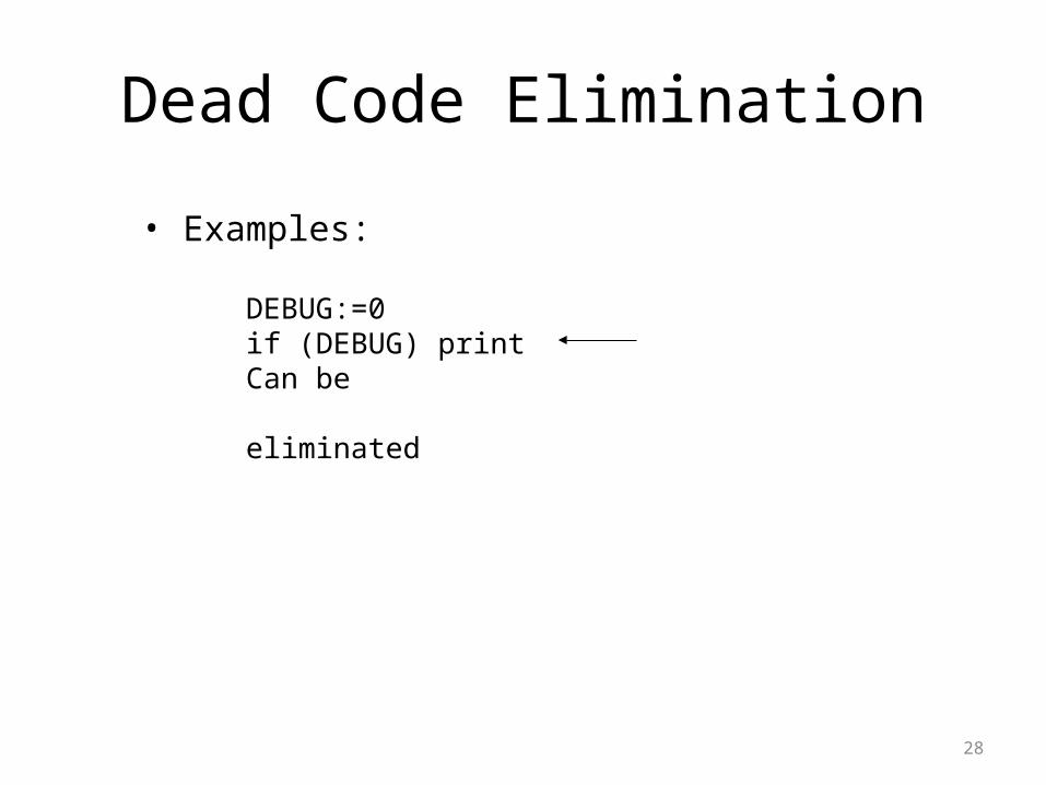
Dead Code Elimination

28

• Examples:

DEBUG:=0if (DEBUG) print Can be

eliminated

Copy Propagation• What does it mean?

– Given an assignment x = y, replace later uses of x with uses of y, provided there are no intervening assignments to x or y.

• When is it performed?– At any level, but usually early in the optimization

process.

• What is the result? – Smaller code

29

Copy Propagation

• f := g are called copy statements or copies• Use of g for f, whenever possible after copy

statement

Example:x[i] = a; x[i] = a;

sum = x[i] + a; sum = a + a;

• May not appear to be code improvement, but opens up scope for other optimizations.

30

Local Copy Propagation

• Local copy propagation– Performed within basic blocks– Algorithm sketch:

• traverse BB from top to bottom• maintain table of copies encountered so far• modify applicable instructions as you go

31

Loop Optimization

• Decrease the number of instruction in the inner loop

• Even if we increase no of instructions in the outer loop

• Techniques:– Code motion– Induction variable elimination– Strength reduction

32

Algebraic identities• Worth recognizing single instructions with a constant operand:

A * 1 = A

A * 0 = 0

A / 1 = A

A * 2 = A + A

More delicate with floating-point

• Strength reduction:

A ^ 2 = A * A

33

Replace Multiply by Shift

• A := A * 4;

– Can be replaced by 2-bit left shift (signed/unsigned)

– But must worry about overflow if language does

• A := A / 4;

– If unsigned, can replace with shift right

– But shift right arithmetic is a well-known problem

– Language may allow it anyway (traditional C)

34

Folding Jumps to Jumps

• A jump to an unconditional jump can copy the target address

JNE lab1 ...lab1: JMP lab2

Can be replaced by: JNE lab2

As a result, lab1 may become dead (unreferenced)

35

Jump to Return

• A jump to a return can be replaced by a return JMP lab1

... lab1: RET

– Can be replaced by RET

lab1 may become dead code

36

Local Optimization

37

Optimization of Basic Blocks

• Many structure preserving transformations can be implemented by construction of DAGs of basic blocks

38

Basic blocks and flow graphs• Partition the intermediate code into basic blocks

– The flow of control can only enter the basic block through the first instruction in the block. That is, there are no jumps into the middle of the block.

– Control will leave the block without halting or branching, except possibly at the last instruction in the block.

• The basic blocks become the nodes of a flow graph

Rules for finding leaders

• The first three-address instruction in the intermediate code is a leader.

• Any instruction that is the target of a conditional or unconditional jump is a leader.

• Any instruction that immediately follows a conditional or unconditional jump is a leader.

Intermediate code to set a 10*10 matrix to an identity matrix

Flow graph based on Basic Blocks

DAG representation of Basic Block (BB)

• Leaves are labeled with unique identifier (var name or const)

• Interior nodes are labeled by an operator symbol• Nodes optionally have a list of labels (identifiers)• Edges relates operands to the operator (interior

nodes are operator)• Interior node represents computed value

– Identifier in the label are deemed to hold the value

43

Code improving transformations

• We can eliminate local common subexpressions, that is, instructions that compute a value that has already been computed.

• We can eliminate dead code, that is, instructions that compute a value that is never used.

• We can reorder statements that do not depend on one another; such reordering may reduce the time a temporary value needs to be preserved in a register.

• We can apply algebraic laws to reorder operands of three-address instructions, and sometimes t hereby simplify t he computation.

DAG for basic block

DAG for basic block

Array accesses in a DAG• An assignment from an array, like x = a [i], is represented by

creating a node with operator =[] and two children representing the initial value of the array, a0 in this case, and the index i. Variable x becomes a label of this new node.

• An assignment to an array, like a [j] = y, is represented by a new node with operator []= and three children representing a0, j and y. There is no variable labeling this node. What is different is that the creation of this node kills all currently constructed nodes whose value depends on a0. A node that has been killed cannot receive any more labels; that is, it cannot become a common subexpression.

DAG for a sequence of array assignments

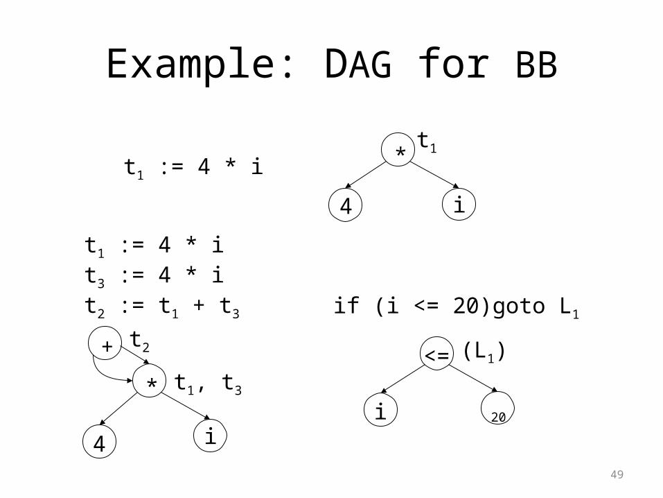
Example: DAG for BB

49

t1 := 4 * it1*

i4

t1 := 4 * it3 := 4 * it2 := t1 + t3

*

i4

+

t1, t3

t2

if (i <= 20)goto L1

<=

i 20

(L1)

Optimization of Basic Blocks

• DAG representation identifies expressions that yield the same result

50

a := b + c

b := b – d

c := c + d

e := b + c

b0 c0 d0

+

++ -a b c

e

Optimization of Basic Blocks

• Dead code elimination: Code generation from DAG eliminates dead code.

51

a := b + c

b := a – d

d := a – d

c := d + c

b is not live

c

a := b + c

d := a - d

c := d + c

b0c0

d0+

-

+

a

b,d×

Rules for reconstructing the basic block from a DAG

• The order of instructions must respect the order of nodes in the DAG. That is, we cannot compute a node's value until we have computed a value for each of its children.

• Assignments to an array must follow all previous assignments to, or evaluations from, the same array, according to the order of these instructions in the original basic block.

• Evaluations of array elements must follow any previous (according to the original block) assignments to the same array. The only permutation allowed is that two evaluations from the same array may be done in either order, as long as neither crosses over an assignment to that array.

• Any use of a variable must follow all previous (according to the original block) procedure calls or indirect assignments through a pointer.

• Any procedure call or indirect assignment through a pointer must follow all previous (according to the original block) evaluations of any variable.

Loop Optimization

53

Loop Optimizations

• Most important set of optimizations– Programs are likely to spend more time in loops

• Presumption: Loop has been identified• Optimizations:

– Loop invariant code removal– Induction variable strength reduction– Induction variable reduction

54

Loops in Flow Graph• Dominators:

A node d of a flow graph G dominates a node n, if every path in G from the initial node to n goes through d.

Represented as: d dom n

Corollaries:Every node dominates itself.The initial node dominates all nodes in G.The entry node of a loop dominates all nodes in the loop.

55

Loops in Flow Graph

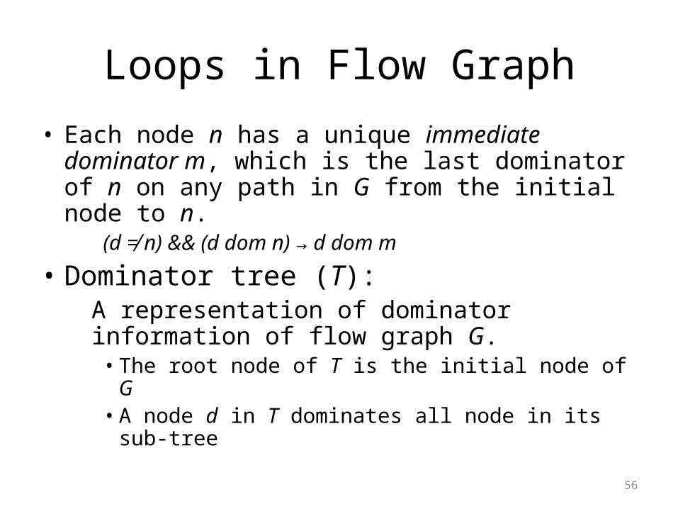
• Each node n has a unique immediate dominator m, which is the last dominator of n on any path in G from the initial node to n.

(d ≠ n) && (d dom n) → d dom m

• Dominator tree (T):A representation of dominator information of flow graph G.

• The root node of T is the initial node of G• A node d in T dominates all node in its sub-tree

56

Example: Loops in Flow Graph

57

1

2 3

4

5 6 7

8 9

Flow Graph Dominator Tree

1

2 3

4

5 6

7

8 9

Loops in Flow Graph

• Natural loops:1. A loop has a single entry point, called the “header”.

Header dominates all node in the loop2. There is at least one path back to the header from the

loop nodes (i.e. there is at least one way to iterate the loop)

• Natural loops can be detected by back edges.• Back edges: edges where the sink node (head) dominates the

source node (tail) in G

58

Inner loops

• Loops having the same header:

59

B3

B1

B2

B4

It is difficult to concludewhich one of {B1, B2, B3}and {B1, B2, B4} is the innerLoop without detailed analysisof code.

Assumption:When two loops have the sameheader they are treated as a singleLoop.

Reducible Flow Graphs

• A flow graph G is reducible iff we can partition the edges in two disjoint sets, often referred as forward edges and back edges, with the following two properties:

1. The forward edges form an acyclic graph in which every node is reachable from the initial node of G

2. The back edges consists only of edges whose heads dominate their tails

60

Example: Reducible Flow Graphs

61

1

2 3

4

5 6

7

8 9

Reducible Flow Graph

2

1

3

Irreducible Flow Graph

The cycle (2,3) can be entered at two different places, nodes 2 and 3

• No back edges, and• The graph is not acyclic

Reducible Flow Graphs

• Key property of a reducible flow graph for loop analysis:– A set of nodes informally regarded as a loop,

must contain a back edge.

Optimization techniques like code motion, induction variable removal, etc cannot be directly applied to irreducible graphs.

62

Loop Optimization

• Loop interchange: exchange inner loops with outer loops

• Loop splitting: attempts to simplify a loop or eliminate dependencies by breaking it into multiple loops which have the same bodies but iterate over different contiguous portions of the index range.

63

Loop Optimization

• Loop fusion: two adjacent loops would iterate the same number of times, their bodies can be combined as long as they make no reference to each other's data

• Loop fission: break a loop into multiple loops over the same index range but each taking only a part of the loop's body.

• Loop unrolling: duplicates the body of the loop multiple times

64

Loop Optimization

• Pre-Header:– Targeted to hold statements that

are moved out of the loop– A basic block which has only the

header as successor– Control flow that used to enter

the loop from outside the loop, through the header, enters the loop from the pre-header

65

Header

loop L

Header

loop L

Pre-header

Example: Induction Variable Strength Reduction

66

r5 = r4 - 3 r4 = r4 + 1

r7 = r4 *r9

r6 = r4 << 2

new_reg = r4 * r9new_inc = r9

r5 = r4 - 3 r4 = r4 + 1

new_reg += new_inc r7 = new_reg

r6 = r4 << 2

Induction Variable Elimination• Remove unnecessary basic induction variables from the loop

by substituting uses with another basic induction variable.• Rules:

– Find two basic induction variables, x and y– x and y in the same family

• Incremented at the same place– Increments are equal– Initial values are equal– x is not live at exit of loop– For each BB where x is defined, there is no use of x between the first

and the last definition of y

67

Example: Induction Variable Elimination

68

r1 = 0r2 = 0

r1 = r1 - 1r2 = r2 -1

r9 = r2 + r4 r7 = r1 * r9

r4 = *(r1)

*r2 = r7

r2 = 0

r2 = r2 - 1

r9 = r2 + r4 r7 = r2 * r9

r4 = *(r2)

*r7 = r2

69

Data Flow Analysis

70

Data Flow AnalysisData flow analysis is used to collect information

about the flow of data values across basic blocks.

• Dominator analysis collected global information regarding the program’s structure

• For performing global code optimizations global information must be collected regarding values of program values.– Local optimizations involve statements from same basic block

– Global optimizations involve statements from different basic blocks data flow analysis is performed to collect global information that drives global optimizations

71

Local and Global Optimization

Applications of Data Flow Analysis• Applicability of code optimizations• Symbolic debugging of code• Static error checking• Type inference• …….

72

1. Reaching DefinitionsDefinition d of variable v: a statement d that assigns a value

to v.Use of variable v: reference to value of v in an expression

evaluation.

Definition d of variable v reaches a point p if there exists a path from immediately after d to p such that definition d is not killed along the path.

Definition d is killed along a path between two points if there exists an assignment to variable v along the path.

73

Example

74

d reaches u along path2 & d does not reach u along path1

Since there exists a path from d to u along which d is not killed (i.e., path2), d reaches u.

Reaching Definitions Contd.Unambiguous Definition: X = ….;Ambiguous Definition: *p = ….; p may point to

X

For computing reaching definitions, typically we only consider kills by unambiguous definitions.

75

X=..

*p=..

Does definition of X reach here ? Yes

Computing Reaching DefinitionsAt each program point p, we compute the set of

definitions that reach point p.Reaching definitions are computed by solving a

system of equations (data flow equations).

76

d1: X=…

IN[B]

OUT[B]

GEN[B] ={d1}KILL[B]={d2,d3}

d2: X=…

d3: X=…

Data Flow Equations

77

GEN[B]: Definitions within B that reach the end of B.KILL[B]: Definitions that never reach the end of B due to redefinitions of variables in B.

IN[B]: Definitions that reach B’s entry.OUT[B]: Definitions that reach B’s exit.

Reaching Definitions Contd.• Forward problem – information flows

forward in the direction of edges.• May problem – there is a path along which

definition reaches a point but it does not always reach the point.

Therefore in a May problem the meet operator is the Union operator.

78

Applications of Reaching Definitions

• Constant Propagation/folding

• Copy Propagation

79

2. Available ExpressionsAn expression is generated at a point if it is computed at that

point.An expression is killed by redefinitions of operands of the

expression.

An expression A+B is available at a point if every path from the start node to the point evaluates A+B and after the last evaluation of A+B on each path there is no redefinition of either A or B (i.e., A+B is not killed).

80

Available Expressions

Available expressions problem computes: at each program point the set of expressions available at that point.

81

Data Flow Equations

82

GEN[B]: Expressions computed within B that are available at the end of B.KILL[B]: Expressions whose operands are redefined in B.

IN[B]: Expressions available at B’s entry.OUT[B]: Expressions available at B’s exit.

Available Expressions Contd.• Forward problem – information flows

forward in the direction of edges.• Must problem – expression is definitely

available at a point along all paths. Therefore in a Must problem the meet

operator is the Intersection operator.• Application:

A

83

3. Live Variable AnalysisA path is X-clear is it contains no definition of X.A variable X is live at point p if there exists a X-clear path

from p to a use of X; otherwise X is dead at p.

84

Live Variable Analysis Computes: At each program point p identify the set of variables that are live at p.

Data Flow Equations

85

GEN[B]: Variables that are used in B prior to their definition in B.KILL[B]: Variables definitely assigned value in B before any use of that variable in B.

IN[B]: Variables live at B’s entry.OUT[B]: Variables live at B’s exit.

Live Variables Contd.• Backward problem – information flows

backward in reverse of the direction of edges.

• May problem – there exists a path along which a use is encountered.

Therefore in a May problem the meet operator is the Union operator.

86

Applications of Live Variables• Register Allocation

• Dead Code Elimination

• Code Motion Out of Loops

87

4. Very Busy ExpressionsA expression A+B is very busy at point p if for all paths

starting at p and ending at the end of the program, an evaluation of A+B appears before any definition of A or B.

88

Application: Code Size Reduction

Compute for each program point the set of very busy expressions at the point.

Data Flow Equations

89

GEN[B]: Expression computed in B and variables used in the expression are not redefined in B prior to expression’s evaluation in B.KILL[B]: Expressions that use variables that are redefined in B.

IN[B]: Expressions very busy at B’s entry.OUT[B]: Expressions very busy at B’s exit.

Very Busy Expressions Contd.• Backward problem – information flows

backward in reverse of the direction of edges.

• Must problem – expressions must be computed along all paths.

Therefore in a Must problem the meet operator is the Intersection operator.

90

Summary

May/Union Must/Intersection

Forward Reaching Definitions

Available Expressions

Backward Live Variables

Very Busy Expressions

91