
Code Blocks Not Required—Dynamo for the Rest of...
40
Page 1 AR20427 Code Blocks Not Required—Dynamo for the Rest of Us Paul F. Aubin Paul F. Aubin Consulting Services, Inc. Description If you use Revit software every day as your primary production tool, you may often run into tedious tasks that you wish you could accomplish more quickly and efficiently. Have you heard that the Dynamo extension can help? But what if you’re not a programmer? Far too many tutorials start by dragging nodes and then end up writing code. If you’ve been frustrated trying to learn Dynamo because it seems all you ever see are code blocks, do not fear—this class uses NO code blocks. We will explore some very practical things you can do to automate your Revit software workflow, all with existing nodes. I repeat, there are no code blocks in this session. Just nodes and wires (and some logic). So, if you want to get a solid introduction to Dynamo for Revit software and come away with some practical examples that you can do back in the office without learning a ton of code, this is the class for you! This session features Revit, Dynamo, and Revit Architecture. Your AU Expert Paul F. Aubin is the author of many Revit book titles including the widely acclaimed: The Aubin Academy Series, Renaissance Revit and Revit video training at www.lynda.com/paulaubin. Paul is an independent architectural consultant providing Revit® for Architecture implementation, training, and support services. Paul’s involvement in the architectural profession spans over 25 years, with experience in design, production, CAD management, mentoring, coaching and training. He is an active member of the Autodesk user community, an Expert Elite and is a top-rated repeat speaker at Autodesk University, Revit Technology Conference and Midwest University. His diverse experience in architectural firms, as a CAD manager, and an educator gives his writing and his classroom instruction a fresh and credible focus. Paul is an associate member of the American Institute of Architects and lives in Chicago with his wife and three children. Learning Objectives • Learn how to use Dynamo to input parameters in custom Revit families • Learn how to apply sequential numbering to model elements • Learn how to export Revit data to Excel, manipulate it, and write it back to Revit • Learn how to manage sheets and views in a Revit project
Transcript of Code Blocks Not Required—Dynamo for the Rest of...

Page 1
AR20427
Code Blocks Not Required—Dynamo for the Rest of Us Paul F. Aubin Paul F. Aubin Consulting Services, Inc.
Description If you use Revit software every day as your primary production tool, you may often run into tedious tasks that you wish you could accomplish more quickly and efficiently. Have you heard that the Dynamo extension can help? But what if you’re not a programmer? Far too many tutorials start by dragging nodes and then end up writing code. If you’ve been frustrated trying to learn Dynamo because it seems all you ever see are code blocks, do not fear—this class uses NO code blocks. We will explore some very practical things you can do to automate your Revit software workflow, all with existing nodes. I repeat, there are no code blocks in this session. Just nodes and wires (and some logic). So, if you want to get a solid introduction to Dynamo for Revit software and come away with some practical examples that you can do back in the office without learning a ton of code, this is the class for you! This session features Revit, Dynamo, and Revit Architecture.
Your AU Expert Paul F. Aubin is the author of many Revit book titles including the widely acclaimed: The Aubin Academy Series, Renaissance Revit and Revit video training at www.lynda.com/paulaubin. Paul is an independent architectural consultant providing Revit® for Architecture implementation, training, and support services. Paul’s involvement in the architectural profession spans over 25 years, with experience in design, production, CAD management, mentoring, coaching and training. He is an active member of the Autodesk user community, an Expert Elite and is a top-rated repeat speaker at Autodesk University, Revit Technology Conference and Midwest University. His diverse experience in architectural firms, as a CAD manager, and an educator gives his writing and his classroom instruction a fresh and credible focus. Paul is an associate member of the American Institute of Architects and lives in Chicago with his wife and three children.
Learning Objectives • Learn how to use Dynamo to input parameters in custom Revit families
• Learn how to apply sequential numbering to model elements
• Learn how to export Revit data to Excel, manipulate it, and write it back to Revit
• Learn how to manage sheets and views in a Revit project
Code Blocks Not Required—Dynamo for the Rest of Us
Page 2
Introduction This session is for beginners. This means that I will start here with some of the basics. If you are already using Dynamo and creating your own graphs, then this first topic and many of the examples that follow will be review for you. But if you are like me, there are always tidbits you can learn even when reviewing familiar material.
Dynamo Interface This topic will cover the critical aspects of the Dynamo interface, starting with installing, launching and running the program and then looking at the key aspects of using the Dynamo environment.
Installing Dynamo Dynamo comes in two varieties. There is a stand-alone version called: Dynamo Studio. This product is available from Autodesk on a subscription model. You pay an annual fee and it runs as a stand-alone application. Dynamo Studio does not interface directly with Revit. Therefore, we will not be using Dynamo Studio in this session. Dynamo for Revit installs as an add-in to the Revit application. If you have Revit 2017, it is already installed and is accessed from the Manage tab. If you have 2016 or 2015, you can download Dynamo for Revit for free and install it. It will show up on the Add-ins tab in these versions. Visit: http://dynamobim.com/ and then click the “Download Dynamo” link to learn more. This session will focus on Dynamo for Revit and will showcase Dynamo version 1.2 running in Revit 2017.
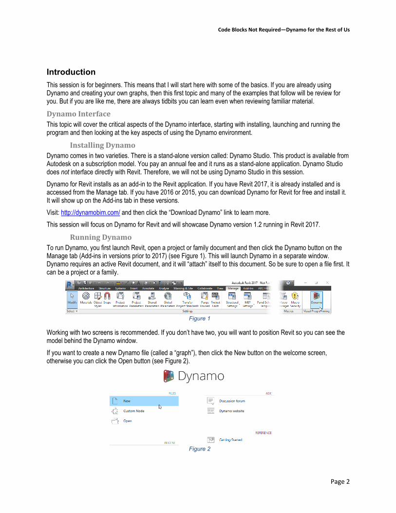
Running Dynamo To run Dynamo, you first launch Revit, open a project or family document and then click the Dynamo button on the Manage tab (Add-ins in versions prior to 2017) (see Figure 1). This will launch Dynamo in a separate window. Dynamo requires an active Revit document, and it will “attach” itself to this document. So be sure to open a file first. It can be a project or a family.
Figure 1
Working with two screens is recommended. If you don’t have two, you will want to position Revit so you can see the model behind the Dynamo window. If you want to create a new Dynamo file (called a “graph”), then click the New button on the welcome screen, otherwise you can click the Open button (see Figure 2).
Figure 2

Code Blocks Not Required—Dynamo for the Rest of Us
Page 3
The Dynamo interface will load with menus across the top, the library on the left and the main graph editing window filling the remainder of the screen. Some navigation tools will appear in the upper-right. At the bottom of the screen is the execution options button (see Figure 3).
Figure 3
Your library may not match the figure. Dynamo is extensible and many users of the community make their own custom nodes and make them available in “packages” to other users. Any installed packages will appear in your library panel intermingled with the default ones. If you hover over a library category, it will indicate if it is a package by showing the letters: “PKG”. The Add button at the base of the library can be used to add more packages to your install as can the Package menu on the menu bar.
Nodes and wires Creating a Dynamo script (or graph) uses “Nodes” and “Wires.” Nodes are prebuilt blocks of code that perform a single discreet action or function. Wires are used to connect nodes together and build the “flow” of the graph moving data from left to right and from node to node (see Figure 4).
Figure 4
To place a node, simply locate it in the library and click on its name (see the left side of Figure 5). The node will appear in the canvas. You can move it around by dragging it by the titlebar. To add a wire, click on one of the “ports” on the node. Ports appear on the left and right sides of nodes. Data in a Dynamo graph flows from left to right. The left side contains the “inputs” and the right side has the “outputs.”

Code Blocks Not Required—Dynamo for the Rest of Us
Page 4
To wire up your nodes, simple click on the port of one node, a wire will extend out of the port as you move your mouse. Click on another port to finish the wire and connect the two ports (see the right side of Figure 5).
Figure 5
Inputs can only have one wire. But multiple wires can be connected to outputs allowing output values to feed into several other locations of the graph.
Finding Nodes You can browse the library by clicking on the category headings to see what is stored within them. But Dynamo contains LOTS of nodes. So browsing this way can be time consuming. So an alternative is to search for nodes. There is a Search field at the top of the library and you can also right-click in the canvas to get a search field on the context menu (see Figure 6).
Figure 6
However, the trouble with searching if you are a beginner is knowing what to search for… So I do recommend that you take some time initially to browse the library and get familiar with the included nodes and overall library structure. In the graphs that follow, I indicate where each node is located in the library for your convenience.
Hello World Once you are familiar with the overall interface, you will want to create your first graph. Programmers always like to show the “Hello World” example as an “ice-breaker.” In other words, something really simple to get quick results.
Simple Text On the library, click the Core branch and then click the Input branch. This branch contains several types of input nodes. These are nodes that you use to feed information to your graph. Click the String node to add it to the canvas (see Figure 7).

Code Blocks Not Required—Dynamo for the Rest of Us
Page 5
Figure 7
Within a String node you can input any text you like. Programmers like to refer to text as “strings.” So you can type in anything you want into a String node. And even if you type in numbers, the graph will interpret them as text only. (We’ll see numerical input below). In the String node, type: Hello World. To finish, click away from the node, don’t press ENTER. If you press ENTER, it will stay in the node and wrap to the next line. Now let’s grab a “Watch” node. Watch nodes are useful to “report” the output at points along the graph. To find it in the library, expand the Core branch and then the View branch. Click on the Watch node to add one. Drag it to the right of the String node and then wire the output of the String to the input of the Watch (see Figure 8).
Figure 8
Very exciting! Well, that is a complete graph, just not very useful or exciting. Let’s vary it a bit. Add another String node. Type “Hello” in the first one and “World” in the second. The Watch will still be wired to the original node and will now only report “Hello.” To put the two together, remember that we cannot put two outputs into a single input. If you try to wire “World” to the Watch, it will replace the wire from “Hello.” So instead, we need another node to combine them first.
Combining Values So how do we combine them? Well there are lots of ways. Here’s a simple one.

Code Blocks Not Required—Dynamo for the Rest of Us
Page 6
On the Operators branch of the library, click the + node. This has two inputs: x and y. These can be anything (kind of like algebra class…) Wire “Hello” into x and “World” into y. Then wire the output of + to the input of the Watch node (see Figure 9).
Figure 9
Notice that it is quite literal and will report “HelloWorld” as the result. You can edit the first String node and add a space at the end of “Hello” to fix that. The graph will update immediately. Again, this is not too exciting, but even this simple example shows how data flows through the graph. Let’s take it a little further. Since we have a + node, what about some numerical input? SAMPLE FILE: You can open a file completed to this point named: 01_Hello World_A.dyn.
Numbers In the library, on the Core > Input branch, click on the Number node. Wire the Number node to the y input of the + node. Note the result in the Watch. In this case, Dynamo will happily combine text with numbers, but it will keep the result as text. But if you create a second Number node and wire it in, it will do the math instead (see Figure 10).
Figure 10
SAMPLE FILE: You can open a file completed to this point named: 01_Hello World_B.dyn.
Making Points Using Dynamo to add two numbers may not be faster than your calculator, but there is plenty more that you can do with numbers. The “hello world” of making geometry would be making points. So let’s look at how you can take some

Code Blocks Not Required—Dynamo for the Rest of Us
Page 7
numbers and feed them into the inputs for making points. The Geometry > Point branch has a few options for making points (see Figure 11).
Figure 11
The main difference is in the inputs required. Let’s look at the Point.ByCoordinates. It is the simplest one and only needs an x and y inputs. If you hover your mouse over an input, it will typically tell you what it expects and if there is a default value. In this case, simply placing this node will add a point to the canvas because the default value of both inputs is zero. So you get a point at 0,0. However, if you wire the two Number nodes into the two point inputs, and then change their values, the point will move accordingly (see Figure 12).
Figure 12
SAMPLE FILE: You can open a file completed to this point named: 01_Hello World_C.dyn.
Making a Line When you want to reuse parts of your graph, you can copy and paste. Simple drag a window around all three nodes (four if you have a Watch), and then from the Edit menu, choose: Copy or press CTRL + C. Then from the edit menu, choose: Paste, or press CTRL + V. With the copies still selected, drag them to position them in a convenient location. Since we copied a point, you now have two points in the same spot. Change the number values of the copied point to move it (see Figure 13).
Figure 13

Code Blocks Not Required—Dynamo for the Rest of Us
Page 8
So what to do with two points? How about make a line! In the library, on the Geometry > Line branch, you will find the ByStartPointEndPoint node. Add that to the canvas and wire it up (see Figure 14).
Figure 14
To Watch or not to Watch… The Watch nodes are not necessary here. I like to include them as I am working so that I get feedback as I go. In this case however, you see the points in the 3D canvas. So the Watch nodes really don’t add anything to the graph. You will also notice that Watch nodes have outputs. You can wire from those or go back to the original node and wire from their output. Notice that here, I have done the latter. This makes it easier to remove the Watch nodes later without forcing you to re-wire anything. There is an alternative to Watch nodes. You can instead receive feedback directly from the node itself. When you hover your mouse over a node, it will show a little pop-up (called a “preview bubble”) with the output of that node. There is a small pushpin icon that you can click to keep the preview bubble expanded even as you move your mouse away (see Figure 15).
Figure 15
If you use the preview bubbles, you can eliminate the Watch nodes. Or you can use both. It is up to you. SAMPLE FILE: You can open a file completed to this point named: 01_Hello World_D.dyn.
Draw a Wall Once you have a line, you can use it to make a Revit wall. As you add nodes to the graph, think about what you want to create, add the nodes and then look to see what inputs are required. There are two nodes available for adding

Code Blocks Not Required—Dynamo for the Rest of Us
Page 9
walls. Let’s use the Wall.ByCurveAndLevels node. This is found in the Revit branch of the library under the: Elements > Wall branch. This node has four inputs: c stands for “curve.” To make a wall, we need a path for it follow. In programmer speak this is called a “curve.” This is “curve” in the math class sense of the word. So our line counts as a “curve.” As does anything with two endpoints; either a straight line or a curvy line and Dynamo still thinks of it as a curve. We also need two levels to set the height and a wall type. Starting with the curve, we can wire the output of our Line node above to the c input. For the others, from the Revit > Selection branch, add: two Levels nodes and one Wall Types. Each of these has a drop-down list from which you can make a selection. From the first Levels node, choose: Level 1 and wire it to the startLevel port. Choose: Level 2 from the next one and wire it to: endLevel and then choose any wall type and wire it to the wallType port (see Figure 16).
Figure 16
Types of Geometry Notice that in Dynamo, we still only see the line. To see the wall, you have to look at Revit. A 3D view shows it well. (Again you might have to shuffle your windows around onscreen to see everything). There is a difference between “Dynamo geometry” and “Revit geometry.” Dynamo geometry only appears in the Dynamo environment and is more abstract. You can use Dynamo geometry to create Revit geometry (as we have done here) and vice-versa. But you will not automatically get both. If you want to see a representation of the wall in Dynamo, browse to: Revit > Elements > Element and use the Geometry node. Wire the output of the Wall node into this node (see Figure 17).
Figure 17

Code Blocks Not Required—Dynamo for the Rest of Us
Page 10
If you want to orbit, pan or zoom the 3D preview in Dynamo, use the small toggle icons at the top right to switch to navigation in the 3D view. Then switch back to the graph when you are done.
SAMPLE FILE: You can open a file completed to this point named: 01_Hello World_E.dyn.
Writing Code All of the previous examples can be considered “Hello World” examples in some form or another. They are very basic, introduce you to the interface of Dynamo and allow you to see immediate results. When you are ready to begin actually using Dynamo to do something practical, you will naturally be building graphs that are more complex. In my experience, this is usually where training sessions like this one dive into the deep end of the pool. However, my goal is to stay in the shallow end for the entire session! All I will say about the “deep end” is that the possibilities are truly endless. That is because let’s make no mistake about it, Dynamo IS programming. To be precise, it is “visual programming.” This simply means that the Dynamo environment is designed to shield you from as much of the underlying code as possible. So we have the lovely nodes, prebaked with useful code that do the heavy lifting for us. Mostly. You drag and drop nodes and wire them up. In a nutshell, that’s visual programming. However, it is not as simple as all that most of the time. First, even when using prebuilt nodes, you still have to understand programming and think like a programmer. This is important to get the logic right. And, even though we have this library of nodes, what you will see very soon, (if you have not already seen it) is that many, if not most, Dynamo graphs and Dynamo programmers do use code. This code is placed in Code Block nodes. At least that is what happens most of the time. But the premise of this session is that you can do many useful things in Dynamo without having to use any code. That means that you can build a perfectly functional graph, that performs a useful procedure without the need for Code Blocks. So does this mean that I think that Code Blocks are bad? Or that they are not useful? Certainly not. I think they are incredibly useful. Just not so much for beginners. I think it is rarely a good idea for beginners to concern themselves with Code Blocks (even if they can save time). I believe that the goal initially should be learning how to work in Dynamo first; before worrying about how to build graphs more quickly or efficiently. “Crawl before you walk or run” so to speak. So now that you at least understand at a conceptual level what a Code Block is, you don’t have to give them any more thought for now, because there won’t be any further mention of them here.
Execution At the bottom of the Dynamo screen, you have a pop-up button that controls how the graph will execute. New graphs default to “Automatic.” This means that as soon as you wire up a node, it will run the graph and perform its function. In smaller graphs without much happening, this can be a nice way to make the experience very interactive. However, as your graphs get more complex, you might want to set the execution to “Manual” instead. This make a “Run” button appear. Now the graph will only execute only when you press the Run button (see Figure 18).
Figure 18
We also have the option to “Freeze” individual nodes to control which parts of the graph execute. This is a great way to execute just a portion of your workflow to ensure that things are working the way that you like before moving on downstream. To freeze a node, right-click it. All nodes connected to it downstream will also freeze (see Figure 19).

Code Blocks Not Required—Dynamo for the Rest of Us
Page 11
Figure 19
Finally, if you save a graph in automatic mode, you can still open it in manual mode. To do so, be sure to use the Open command (File menu, or on the start screen) and browse to the file. In the “Open” dialog, there will be a checkbox available at the bottom of the window to open the graph in “Manual Execution Mode” (see Figure 20).
Figure 20
In general, it is often desirable to open Dynamo files this way. This allows you to check the graph, ensure it is correct and optionally freeze certain parts of the workflow before execution.
Placing Individual Revit Families So now that we have gotten some of the basics under our belt, what practical things can we do with Dynamo? A very common task to perform with Dynamo is placing elements in your Revit model. There are nearly limitless approaches to the task, and much of the specifics will depend on the precise goals and expected outcomes. But there will be some common threads. Typically, you will use the selection nodes to choose which Revit item you want to place. Then you will often need to indicate where in the model to place the elements. And in many cases you will want to manipulate the elements during placement as well. In the examples that follow we will showcase a few workflows to get you started with thinking about how to place elements in your Revit projects with Dynamo.
Placing a Single Family Let’s say that you wanted to place a collection of families along a path. This is easy to do directly in Revit if the path is straight or follows an arc; in those situations, you can use the Array command. But not so if it is irregular like a spline or if you have more than one path. In this example, we’ll look at a graph that allows you to draw a spline in Revit, select it in Dynamo and then insert a variable quantity of elements along that selected path. I’ll use trees here, but you can use this graph to place any non-hosted component family.
Create a spline path in Revit Launch Revit, start a new project using the default template and then create a model line. Use the spline shape and draw a curvy path (see Figure 21). Save the project. The default template has an RPC tree family pre-loaded. If the template you are using does not, just make sure that you have a family loaded that you want to repeat along the path. It should be a non-hosted family. Wall-based, or other hosted families will not work in this example.

Code Blocks Not Required—Dynamo for the Rest of Us
Page 12
Figure 21
Launch Dynamo next and then click the New button on the welcome page. Add the following nodes to your canvas:
Library Location Node
Core > Input Number
Core > Input Number Slider
Revit > Selection Select Model Element
Revit > Selection Family Types
Revit > Elements > Element Curves
Revit > Elements > FamilyInstance ByPoint
Geometry > Curve PointAtParameter
You can manually browse to the location indicated and click the node to add it to the canvas, or you can use the Search field instead and type in the node name to find them. Position the nodes and wire them as indicated in Figure 22.
Figure 22
SAMPLE FILE: You can open a starter Revit file for this example named: 02_Place Families_!Start.rvt and a starter Dynamo file named: 02_Place Families_A.dyn
Errors in Nodes Notice that the Select Model Element node is yellow. This indicates that it is currently in an error state. When you have not fed the proper information into a node and Dynamo is therefore unable to process it, it will display the node this way to alert you. Here the problem is simple; we have not selected the spline path yet. The Select button on the

Code Blocks Not Required—Dynamo for the Rest of Us
Page 13
node is used for this purpose. Click it and then in the Revit window, click on the spline element you created above. Assuming that you have the execution mode (noted above) set to: Automatic, it will process immediately and result in the FamilyInstanstance.ByPoint node going into an error state. This time there is a small indicator above the node that you can highlight to get more information. If you do this, you see that the message says “cannot be null.” This is programmer speak for “empty.” We have not chosen a family from the drop-down on the Family Types node yet. So it does not know which family to place (see Figure 23).
Figure 23
Select a family from the drop-down on the Family Types node to clear the error and place an instance of the family in the Revit canvas. I chose an RPC tree family (see Figure 24), but feel free to choose another model component family if you like.
Figure 24
With the graph wired this way, we get one tree at the start of the spline. Also as we noted above, the tree will appear in Revit, but not in the Dynamo canvas unless you add an Element.Geometry node to the graph. (You are welcome to do this if you like).
SAMPLE FILE: You can open a file completed to this point named: 02_Place Families_B.dyn.
Adjust the Graph and the Resulting Revit Model So how did our tree know to be placed at the end of the spline? And how did it know which end? The key is the param input of the Curve.PointAtParameter node. Right now, we are feeding it a single number. You can input any number you want here within the allowable range. What is the allowable range? In the case of the “AtParameter” nodes, the

Code Blocks Not Required—Dynamo for the Rest of Us
Page 14
“parameter” is a value in the range between zero and one. So a value of zero in the Number node (like we have here) puts it at one endpoint, while 1 would put it at the other endpoint. If you want the tree at the midpoint, you can type in: .5. Use: .75 to put it three quarters the way along the curve, etc. Go ahead and try some other inputs.
Building a Range of Numbers But our goal was to have multiple trees spaced evenly along the path. To do this, you need to feed in more than one value in the param port. There are many ways you can do this in Dynamo. Let’s do a very simple range of numbers. In the library, on the Core > List branch, add a Range node to the canvas. You have three inputs here: start, end and step. Since our param input needs a range from zero to one, we will input those values into the Range node. Then we can step by any fractional amount we want. For example, if you start at zero, end at one and step by .5, you get three items in your range. Step by .25, and you will get five, etc. To input these values, we can use Number nodes or the Number Slider we added above. If you hover over each input, a tooltip will tell you the default value (if there is one). Doing this we see that the start input already defaults to zero, so we really only need to change the end input. Rewire the graph to incorporate the Range node as shown in Figure 25. Be sure to change the value of the Number node to: 1.
Figure 25
The Number Slider is nice because you can drag the slider and have the graph update in real-time. However, we need to adjust the settings of the slider to make it work for the range we require. Click the small chevron icon on the left of the slider to reveal its settings. As we noted, we want the Min to be: 0 and the Max to be: 1. For the Step, try a value of: 0.1. and then close the controls by clicking the chevron again (see Figure 26).
Figure 26
SAMPLE FILE: You can open a file completed to this point named: 02_Place Families_C.dyn.
Understanding Lacing Drag the slider down to about .1 or .2. Unfortunately, it will appear as if nothing is happening. This is where we need to understand the structure of the program we are building here a little better and how the data flows through it. You can add some Watch nodes, or simply pin open the preview bubbles that appear when you highlight a node. For the Element.Curves node, we have one item coming out of it. For the Range node we have a list of items. The Curve.PointAtParameter node is matching the one curve to the one list. The list in-turn is giving us its first item (item [0] in this case, because as you will also note, Dynamo uses “zero-based” numbering. Meaning that lists start at index zero, rather than index one). This is why it appears to not be working correctly, even though in reality it is working perfectly.

Code Blocks Not Required—Dynamo for the Rest of Us
Page 15
Now perhaps that is exactly what you want. Perhaps not. Either way we can control what we get for outputs using a concept called: “lacing.” Lacing is Dynamo’s way of matching the values on two or more lists to one another. The default lacing for the Curve.PointAtParameter node is “Shortest.” Shortest lacing will give you the fewest number of pairings. So in this case, a list of one item matched to a list of six yields one paring, and the simplest of the possible pairings, first item to first item (item [0] in each case). If we fed two curves into the curve input and ran the graph again, we would still get a single tree on each curve. However, the tree on the second curve would be placed at location number two (index [1]) from the second list (see Figure 27).
Figure 27
Note that in the figure, I have switched out the Select Model Element node with a Select Model Elements (plural) node. Select Model Element lets you select only one element in the Revit model, while Select Model Elements allows a selection of two or more elements.
There are two other lacing options: Longest and Cross Product. Right-click on a node to change the setting. With longest, the paring process will be the same as shortest for the first items, but when the shorter list is exhausted, the final item on the shorter list will be repeated to ensure a number of pairings equal to the longer list. This does not always give the desired result (see Figure 28).

Code Blocks Not Required—Dynamo for the Rest of Us
Page 16
Figure 28
The final option: Cross Product, matches all possibilities. So you can end up with many pairings! In this case, if you want to add trees to all locations on both paths, then Cross Product would do the trick (see Figure 29).
Figure 29

Code Blocks Not Required—Dynamo for the Rest of Us
Page 17
You may also want to take notice of the structure of the list that is generated by the Curve.PointAtParameter node in each case. The list structure with lacing set to: shortest is a list of lists. The parent list contains two sub-lists. Each of those lists contain a single point. With lacing at longest, we also get a list of lists. But this time there are six lists each with one point. When we go to cross product, we now have 3-level nested list. The top level is two lists that each contain six lists. Those six lists contain a single point each. If you go back to the simpler graph with only the spline path selected, then you can get to the final result with either longest or cross product lacing. And in either case, as you drag the slider, it will now change the step value interactively within the limits set; in other words, you will see the quantity of trees reflect the change as you drag the slider. You can also play with the limits on the slider to vary the resultant quantities. SAMPLE FILE: You can open a file completed to this point named: 02_Place Families_D.dyn.
Placing Multiple Families The previous example placed one or more instances of the same family and type. You may also wish to place more than one family. One of the places where Dynamo really excels is in performing repetitive tasks. In this next example let’s assume you wanted to create a single project file that would serve as a library or “warehouse” file. Users can then open the project file, locate the item they want and more importantly see an instance of each element already inserted onscreen in the file. Then they can simply select the one they need and copy and paste it to their project. Many firms build these so called warehouse files. But without a tool like Dynamo, it can be quite tedious to create one. In the first example, we’ll create a simple wall type warehouse using out-of-the-box wall types. After that, we’ll create a second warehouse using out-of-the-box casework families. There will be similarities in each graph, but some significant differences as well. This is because walls are system families while casework are component (loadable) families. You are likely already familiar with some of the differences between system and non-system families. Well, they differ under the hood in the API as well. Dynamo is really like our bridge to the API, and while visual programming does shield us from much of the API issues and complexities, it does not conceal all of them. So keep in mind that Dynamo can only perform tasks that are possible through the Revit API. It just provides a more accessible way to do so that is easier to learn for many users.
Prepare a Project File To get started you can simply create a new project file from the default template and save it as: Wall Warehouse. You can use any of the default template files. I used the default Architectural template installed with the US Imperial install of Revit for this example.
Repurpose an Old Graph If you followed along with the “Hello World” examples above, then we will actually be able to reuse much of the graph that we built there. Our wall warehouse will need to make points by coordinates, draw lines and then place walls on these “curves.” So if you still have that graph, the easiest thing to do is save it as a new name. I begin many of my Dynamo graphs this way. It saves time and allows you to maintain consistency. I do also re-build them scratch frequently as well, as there is much that can be learned and reinforced by building a new graph for a familiar solution. So either approach is perfectly fine.
Creating a Wall Warehouse The graph is not too complicated. We need to get a list of all of the wall types in the project, create an equal number of lines (curves) for the placement of each one, and then feed this list of wall types into the node that creates the walls. Rather than explain each step of placing and wiring each node, I will instead show you the final graph (see Figure 30), and then explain each of its pieces.
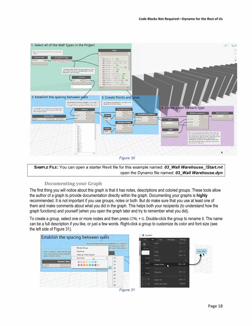
Code Blocks Not Required—Dynamo for the Rest of Us
Page 18
Figure 30
SAMPLE FILE: You can open a starter Revit file for this example named: 03_Wall Warehouse_!Start.rvt open the Dynamo file named: 03_Wall Warehouse.dyn
Documenting your Graph The first thing you will notice about this graph is that it has notes, descriptions and colored groups. These tools allow the author of a graph to provide documentation directly within the graph. Documenting your graphs is highly recommended. It is not important if you use groups, notes or both. But do make sure that you use at least one of them and make comments about what you did in the graph. This helps both your recipients (to understand how the graph functions) and yourself (when you open the graph later and try to remember what you did). To create a group, select one or more nodes and then press CTRL + G. Double-click the group to rename it. The name can be a full description if you like, or just a few words. Right-click a group to customize its color and font size (see the left side of Figure 31).
Figure 31

Code Blocks Not Required—Dynamo for the Rest of Us
Page 19
You can also create a Group from the Edit menu. Use the Edit menu to add notes as well. Or press CTRL + W (see the right side of Figure 31). To customize a note, double-click it. You cannot change the color or size of the note. So if you want to control those things, use a group instead. Now let’s take a look at each group in the graph. Refer back to Figure 30 for the following topics. Each topic will list the nodes used at the end with their locations in the library, but you can also simply search for them instead.
Make a List of All Wall Types Group number 1 wires an Element Types node into an All Elements of Type node. The drop-down list on the first node lists all element types in Revit. Choose: WallType to get a list of all wall types in the current project. This is reflected in the Watch node. The List.Count node shows that this particular project includes 27 wall types. But the nice thing about this is, if you add or delete types, the graph (and the count) will update.
Library Location Node
Core > List Count
Core > View Watch
Revit > Selection Element Types
Revit > Selection All Elements of Type
Establish the Spacing Between Walls Group 2 has only two nodes. Here we are using a Number Slider to interactively set the spacing between the placed walls. This is accomplished by creating a sequence of numbers with a Sequence node. Its start input defaults to zero. So we do not need to feed in anything here. The amount input is how many items you want in the sequence. (These can be numbers or letters incidentally, but we need numbers in this case). So here we feed in the quantity of wall types derived from the Count node above. For the step value, we use the slider to make it interactive. You can adjust the settings of the slider to make it snap to more reasonable settings than the default. I used a maximum value of: 10 with a step of: .5. So with the value of: 5 shown in the figure, we get a sequence of 27 numbers starting at: 0 and ending at: 130 incrementing by 5 each time. Try other values if you like.
Create the Curves You recall from above that Dynamo thinks of any linear shape as a curve. It can be a straight line, an arc or freeform spline. These are all curves. Revit however, only allows walls to follow straight line or circular arc paths. So we must always be sure to know any limitations in Revit and ensure that our graph is built with these in mind. So if you fed an ellipse or spline path for example into the Wall node later, it would fail. In group 3 we are creating two sets of points that will be used to define a series of lines. This part of the graph illustrates an important concept in Dynamo: Most inputs can take either single values or lists! (We saw this in the tree example too, but it is worth highlighting this important fact). If you feed in an individual value, you get a single output. But if you feed in a list, you get a list of outputs! Very cool! So what do we need? Well we have 27 wall types. So we want 27 pairs of X, Y points, 27 lines from the points and ultimately 27 walls based on those lines. How do we achieve this? We simply make sure that we feed in a list to at least one of the inputs. In our case, we only want the X values to vary. We will keep the Y values constant. This will draw our lines and walls along the X axis (horizontally). We need two Point.ByCoordinates nodes. There are two to choose from, one has x and y inputs the other also has z. You can use either one. Just leave z empty and it will default to zero and you get the same result. Since we don’t

Code Blocks Not Required—Dynamo for the Rest of Us
Page 20
want to vary the y inputs, we can use two Number nodes for those inputs and just type in the values we want. Any numbers will work here, but choose a value that sets the length of the walls to a reasonable size. The x port is where we feed in our lists. They will both use the same list: our output from the Sequence node above. Recall that this gave us a list of 27 numbers spaced evenly (by the slider). These will now be used as our x values and more importantly we will end up with 27 sets of points as a result. To complete this group, feed the two Point node outputs into a Line.ByStartPointEndPoint node and we will end up with 27 lines marching off to the right.
Library Location Node
Core > Input Number
Geometry > Point ByCoordinates
Geometry > Line ByStartPointEndPoint
Create Wall Geometry Our final group, group 4 creates the walls. This group mimics what we started with from the “Hello World” example above. We have a Wall.ByCurveAndLevels node. It has four inputs. If you started with the old file, you already have the Levels nodes inserted and wired up. The c input receives the output from the Line node. This will feed in the 27 lines (curves) to create 27 walls. For the wallType input, feed in the list of wall types captured in the first group. That’s it! You should get 27 walls onscreen in Revit. If you want to see them in Dynamo as well, add the optional Element.Geometry node to create the representation in the Dynamo canvas. But this node is not required.
Library Location Node
Revit > Selection Levels
Revit > Elements > Element Geometry
Revit > Elements > Wall ByCurveAndLevels
Creating a Casework Warehouse As noted above, the procedure for system families differs a bit from component (loadable) families. This is true in the Revit interface and certainly in the API and by extension in Dynamo. For one, system families are already built-in to all Revit projects. Component families must be loaded. So if you want to create a library file of families in a component category such as casework, you will need to ensure that you have some loaded. While there are ways to load from external files directly in Dynamo, in this workflow, we will start with a file that has some casework pre-loaded and focus our graph on placement of the families in the project. So before you begin, from the Insert tab, load a bunch of casework families. You do not need to place any of them in the model. That is what we will use Dynamo for. Just load them into the project and save it. For my example, I am loading all of the families from the out-of-the-box library that are contained in the Casework\Base Cabinets folder. I chose these because they are free-standing and do not require wall hosts.
SAMPLE FILE: You can open a starter Revit file named: 04_Casework Warehouse_!Start.rvt and a starter Dynamo file named: 04_Casework Warehouse_A.dyn
and the CSV file: List of Families.csv

Code Blocks Not Required—Dynamo for the Rest of Us
Page 21
As you can see, this graph is a bit more complex than the previous one. It still takes a list of types and computes a series of X and Y coordinates for placement, but his graph has two new features not covered in the previous ones. First, to get the list of families, we are reading a text file from disk. And when processing the coordinates, we will also use a custom node from a downloadable “Package.” A Package is like a plug-in for Dynamo. Dynamo has a very active user community and many community members have extended the functionality of Dynamo by making Packages available. Once you install a Package, its nodes work exactly like the out-of-the-box ones, so there is no reason to shy away from them. Here is an overall look at the whole graph. In the topics that follow, we’ll explore each numbered group (see Figure 32).
Figure 32
Loading Information from an External File In the first group, I am loading an external text file. This is a quick way to get a list of all the families in the project and use it to get their types. Later we will see that there is a node to query all of the types from a list of families, but there is not a node to get a list of all the families loaded in the project. There might be external Packages out there with such a node, and you are welcome to explore. For now, we’ll save further discussion of Packages for the example showcased below. In the meantime, using an external file to get a list of families is quick, easy and effective. You can read an external CSV formatted text file or an Excel file. The process and nodes required are similar for each. Since I am doing just a simple list here, I went with CSV for this example. To create the list, you can of course type it manually in: Notepad, but it is quicker to use SnagIt (or similar) and do a text capture or use a command prompt and the DIR command to export a list of families from a folder in Windows Explorer. I will leave the specific choice of process to you. Once you have the file, you can Browse to it with a File Path node (see Figure 33).
Figure 33
File Path points to the file on disk. But to read it into Dynamo and access the data it contains requires two nodes: File.FromPath and CSV.ReadFromFile.

Code Blocks Not Required—Dynamo for the Rest of Us
Page 22
When you read a file from CSV (or from Excel) it will create a list of lists. Each sub-list will contain one row of data from the comma-separated file in its own list. This will be the case even if there is only one piece of information per row like we have here (see the preview bubble on the left side of Figure 34).
Figure 34
That data structure might be what you want, but in many cases you would rather have a list organized by column instead. To do this, we need to transpose it (see the Watch node on the right side of Figure 34). Transpose simply reverses the data structure to organize by columns instead of rows or vice-versa. Once we have read our file and transposed its data, we can feed that into the next node in group 2. Here we have two nodes: Family.ByName which takes a name or list of names and Family.Types which reports all of the types within each family coming in. So this gives us a complete list of the all the types from all of the casework families on our list. The structure of the list is a three-tiered nested list.
Library Location Node
Core > Input File Path
Core > File File.FromPath
Core > File > CSV ReadFromFile
Core > List Transpose
Revit > Elements > Family ByName
Revit > Elements > Family Types
An Alternative to Reading an External File You may be wondering if there is an alternative to creating a list of families externally to the graph and reading it in. Well, it is possible to use a List.Create node and build a custom list. You use the small + icon on the node to add inputs. The trouble is, as you can see in Figure 35, you would have to add many items to your list and manually choose each family type from the drop-down. So this is quite tedious and I therefore believe creating and then reading the CSV file is much better choice.

Code Blocks Not Required—Dynamo for the Rest of Us
Page 23
Figure 35
SAMPLE FILE: You can open this Dynamo file named: 04_Casework Warehouse_B.dyn This graph also showcases the older style usage of List.Map to apply functions to nested lists.
Getting the Widths of Family Types In group 3 we are getting the widths from the type properties. As noted in the previous topic, the list currently has a three-level hierarchy. For now, we want to drop that to two levels: a parent list containing lists for each family. The elements on the sub-lists will be the values for the widths of each type. To get those, we can use GetParameterValueByName. This node gets the value of any parameter from any element or type in your model. In this case, we are asking the types what their respective width values are (see Figure 36).
Figure 36
Library Location Node
Core > Input Number
Core > Input String
Core > List Flatten

Code Blocks Not Required—Dynamo for the Rest of Us
Page 24
Revit > Elements > Element GetParameterValueByName
Determine the Spacing of Elements To determine the spacing of elements we will start with the X direction. The list we just generated in the previous group is how wide each family type is. To this, we can add a constant value to maintain a consistent amount of space between each item. If you look at group 4, this is done with the first two nodes. A slider is used here to make it easier to change the spacing interactively (see Figure 37).
Figure 37
This gives us the width plus spacing. But we need to start the first item in each list at zero. This is accomplished with the List.AddItemToFront node. However, if we use it directly, it will add the item to the main list. We want to add zero to each sub-list. This is accomplished by applying the effect with “Levels.” You can click the small little triangle icon on the input, and then check the “Use Levels” checkbox. It will default to @L2 which means apply the function to the level 2 list. This is what we want here. If you need it to apply to a different level, click the small spinner icons to choose a different level. (In older versions of Dynamo, you would need to use List.Map to achieve similar functionality). Following this node, we now have too many items on each list. So now we will use a List.DropItems node to remove the last item from each nested list. Check “use Levels” on this one as well to apply the function to the nested list. The amount input on List.DropItems takes either positive or negative numbers. Positive numbers drop items from the start of the list, while negative numbers drop items at the end of the list. So here we are using negative one to remove the last item on each list. This gives us the distances we need to determine the X spacing, but they are not the actual coordinates yet. We will explore how to get there in group 6 below. Meanwhile, let’s take a moment to build the spacing in the Y direction.
Library Location Node
Core > Input Number Slider

Code Blocks Not Required—Dynamo for the Rest of Us
Page 25
Library Location Node
Core > Input Number
Operators +
Core > List AddItemToFront
Core > List DropItems
Working in parallel, we have the nodes that determine the Y spacing. If you return to the start of the graph and do another GetParameterValueByName for the: Depth, we find that since these are casework elements, almost all of them use the same depth for each type. The only exception is the corner cabinet which is a little larger. Therefore, I have decided that it will be simpler to use a consistent value for the Y direction. Furthermore, we can use a slider to change the value and then apply it directly to the Y coordinates using simple multiplication instead of nested lists.
Figure 38
Start by building a Range (see Figure 38). It starts at zero and the end receives the output from the Count of original type list. Now recall that this is a nested list containing lists of families that in turn list out all of the types. If we count this list, we get the quantity of parent lists (the number of families, which is what we want here). If you wanted the count of the number of types, you would use the Count node with a List.Map instead. We can leave the step alone since it defaults to 1 which is what we need here. Feed this range of values into a multiplication node and multiply it by the slider. If you want to ensure that there is always enough room for each family, set the minimum value of the slider to something like: 4. This will ensure that it is a little larger than the largest depth of the families we are using. This gives us results that are usable directly as our Y coordinates. So we will feed them into the y port of our Point.ByCoordinates node below. But as noted above, we still need to do a little more work on our X values.
Library Location Node
Core > Input Number Slider
Core > Input Number

Code Blocks Not Required—Dynamo for the Rest of Us
Page 26
Library Location Node
Operators *
Core > List Range
Core > List Count
Using a Package Node For the X direction we have a choice. The simplest way to do it would be to do it exactly like we did with Y values. To do this, we would choose a minimum spacing value that was wider than the largest element’s width plus a little more to provide some space in-between. This would ensure that there was enough room for each element, but some would have less space between them than others, but the center-to-center distances would always be equal. The other option is the one I have opted for here. I would prefer that the space between elements always be equal, therefore the center-to-center spacing will vary with the widths of each element type. This means that we cannot use simple multiplication like we did with the Y values. Instead, we have to do a running addition of the values computed in group 4 above. Consider list [1] as an example. The first element will be placed at: 0. The next one is at: 0 + 3, the next one is the sum of the first three values: 0 + 3 + 3.5, or 6.5 and so on. I have had some success with this using a List.Scan node for this is other graphs. I decided to show a different approach here. I have turned to a node from the LunchBox Package called: LunchBox Mass Addition. To locate a Package, open the Packages menu and choose: Search for a Package (see the left side of Figure 39). In the “Online Package Search” dialog that appears, type: lunchbox into the Search field. When LunchBox for Dynamo appears, click the arrow icon on the left to download and install it (see the middle of Figure 39). Click OK in any messages that appear to confirm download and installation. (LunchBox will alert you that it has “dependencies.” It is safe to click OK here and dismiss that warning). Once installation is complete, you will see a new branch for LunchBox in your library panel. If you hover over the name, the letters PKG will appear to the right of the name. This indicates that it is a Package (see the right side of Figure 39).
Figure 39
There are hundreds of Packages available that perform all sorts of useful functions. Feel free to explore and install others if you wish. Keep in mind that like any community driven initiative, the quality and utility of Packages will vary. I tend to only install a Package if it has a node that fulfills a certain task I am trying to solve in my graph. If you are concerned about installing Packages, just take a few moments to do a Google search on the Package you are considering. The Dynamo community is very active and you will likely find many posts about the Package you are

Code Blocks Not Required—Dynamo for the Rest of Us
Page 27
considering with users giving you the straight talk on the best ones available out there. And of course you can always uninstall ones you no longer find useful.
Using LunchBox to Create a Running Sum Now that we have the LunchBox Package installed, we can use its nodes just like any other. In this case we need LunchBox Mass Addition. We want it to perform its function on the nested list, so we will check the “Use Levels” option again. A Watch node will reveal that it has correctly given us a running sum of the values for our X coordinates (see the left side of Figure 40).
Figure 40
Creating Points and Placing Family Instances Group 7 completes the graph and places our family instances. To do this, we need to go all the way back to the list of types generated in group 2. We want to place one of each of the types on the that list. To do that, we have to take our lists of X and Y values and create points from them. A Point.ByCoordinates node will be used for this. As we noted above, you can use the one that asks for only x and y or the one that wants x, y and z. Just leave z blank to place them all at the default of zero. Feed the results from the List.Map in group 6 into x and the results from the multiplication node in group 5 into y. Both of these are hierarchical lists and more importantly, their respective structures match, so we get a nice grid of points in the quantities required (see Figure 41).
Figure 41

Code Blocks Not Required—Dynamo for the Rest of Us
Page 28
But now that we have this grid of points, the hierarchy is no longer required. And in fact, if we keep it, we will not get families placed properly. So we need to flatten both the list of points coming out of the point node and the list of types coming out of the Family.Types node back in group 2. There are two flatten nodes in the out-of-the-box library. One is on the Core > List branch and includes the amt input so that you can tell it how many levels of lists to flatten. There is also a simple Flatten node located in the: Builtin branch of the library. This one will flatten the entire list regardless of its structure. This is the one we will use here. (However, if you check “Use Levels” there really is not much difference between these two nodes anymore). Add two of them and flatten the output from the Family.Types node and the output of the Point.ByCoordinates node. Finally feed these flattened outputs into the FamilyInstance.ByPoint node to create the families in Revit.
Library Location Node
LunchBox > Math > Operators LunchBox Mass Addition
Builtin Flatten
Geometry > Point ByCoordinates
Revit > Elements > FamilyInstance ByPoint
Once again, the Element.Geometry node is optional but it is not recommended in this case. The reason is that it will add significantly to the amount of time it takes to process the graph. So leave it out and use the Revit window to see the results. So now you have three different approaches to placing Revit families. If you plan to use Dynamo with Revit, there is a good chance that you will need to place elements at some point, so techniques from one or more of those examples should prove helpful. But these examples are by no means exhaustive. There are many other ways you can place Revit elements and interact with those that are already in your model. In the next topic, we will explore a little bit of both.
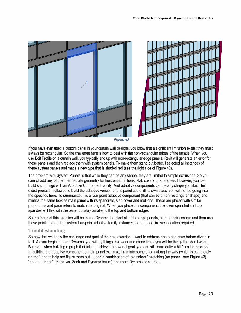
Processing Data The goal of the final example involves a curtain wall façade and using Dynamo to help us place many custom shaped curtain panels. The façade has an irregular shape along the edges as it climbs the height of the building. To get the custom curtain wall shape, I used Edit Profile. The curtain panel being used in the design is a custom curtain panel family. The family has a lower horizontal spandrel, a glazing area and then another horizontal band across the top with a slab cover. Instead of using Revit mullions, the mullions are modeled directly in the panel family and wrap around the edges as well as horizontally dividing the three zones of the panel design (see the left side of Figure 42).
Code Blocks Not Required—Dynamo for the Rest of Us
Page 29
Figure 42
If you have ever used a custom panel in your curtain wall designs, you know that a significant limitation exists; they must always be rectangular. So the challenge here is how to deal with the non-rectangular edges of the façade. When you use Edit Profile on a curtain wall, you typically end up with non-rectangular edge panels. Revit will generate an error for these panels and then replace them with system panels. To make them stand out better, I selected all instances of these system panels and made a new type that is shaded red (see the right side of Figure 42). The problem with System Panels is that while they can be any shape, they are limited to simple extrusions. So you cannot add any of the intermediate geometry for horizontal mullions, slab covers or spandrels. However, you can build such things with an Adaptive Component family. And adaptive components can be any shape you like. The exact process I followed to build the adaptive version of this panel could fill its own class, so I will not be going into the specifics here. To summarize: it is a four-point adaptive component (that can be a non-rectangular shape) and mimics the same look as main panel with its spandrels, slab cover and mullions. These are placed with similar proportions and parameters to match the original. When you place this component, the lower spandrel and top spandrel will flex with the panel but stay parallel to the top and bottom edges. So the focus of this exercise will be to use Dynamo to select all of the edge panels, extract their corners and then use those points to add the custom four-point adaptive family instances to the model in each location required.
Troubleshooting So now that we know the challenge and goal of the next exercise, I want to address one other issue before diving in to it. As you begin to learn Dynamo, you will try things that work and many times you will try things that don’t work. But even when building a graph that fails to achieve the overall goal, you can still learn quite a bit from the process. In building the adaptive component curtain panel exercise, I ran into some snags along the way (which is completely normal) and to help me figure them out, I used a combination of “old school” sketching (on paper - see Figure 43), “phone a friend” (thank you Zach and Dynamo forum) and more Dynamo or course!

Code Blocks Not Required—Dynamo for the Rest of Us
Page 30
Figure 43
As I worked through it, I thought that one of the “troubleshooting” graphs I created while building the solution was actually educational in itself. So I decided to include that one here as a preliminary to the curtain panel edges graph that we have just outlined. If you would rather skip right to the curtain panel example, you can skip down to the “Placing Adaptive Components” heading below.
Numbering Elements While the ultimate goal in this exercise is to add the adaptive components for the edge panels, let’s start with the “troubleshooting” graph I noted above. While working out this exercise, I was having trouble determining if the points were being calculated correctly and also having trouble getting the adaptive components placed. To help me troubleshoot this, I found it useful to identify each edge panel in the model uniquely. The easiest way to do this was to assign each one a unique value in their Mark field. Furthermore, one of the Dynamo nodes we will be using will trace the shape of each edge panel. In some cases, this yields 4 points (which we want) while in other cases it yields a different quantity (usually 6, which we don’t want). So in addition to being able to assign a unique value to each panel, I wanted to easily point out which were four points and which were more.
SAMPLE FILE: You can open a starter Revit file named: 05_Curtain Wall Facade_!Start.rvt open the Dynamo file named: 05_Curtain Wall Façade_A.dyn
Select Curtain Panels and Process them The first part of the graph uses a Family Types node and an All Elements of Family Type to select all of the curtain panels on the edge. In the initial state of the file, this is: System Panel: Solid (Red). Next we have a CurtainPanel.Boundaries node. This node traces the outline of the curtain panel with a polycurve. This will create a nested list of lists. So the next node flattens the list and then using a PolyCurve.NumberOfCurves, we find out how many curves are contained in each polycurve. The final node in group 1 is an “equal to” node. This node asks if input x is equal to input y. It outputs a list of true or false values (see Figure 44).

Code Blocks Not Required—Dynamo for the Rest of Us
Page 31
Figure 44
Library Location Node
BuiltIn Flatten
Core > Input Number
Geometry > Polycurve NumberOfCurves
Operators ==
Operators +
Revit > Selection Family Types
Revit > Selection All Elements of Type
Revit > Elements > Curtain Panel Boundaries
Build a Mark value from a Number Sequence and Conditional Suffixes In group 2 at the bottom of the figure, we are creating the desired mark values. We start with a Sequence node. Its start input defaults to 0. This is fine for our purposes, so no need for an input there. The amount input is for how many items you want in the sequence. In this case, a List.Count from the panel selection above will give us the correct value and will adjust automatically if the number of panels changes as you re-run the graph. The output here will be numerical. In any kind of programming, including Dynamo, Data types are very important. If you have even gotten an “Insistent Units” message while building content in the family editor, then you know what I am talking about.

Code Blocks Not Required—Dynamo for the Rest of Us
Page 32
If you haven’t, just know that data types must match and if they don’t you have to convert them. So since the “Mark” field that we will be writing this data to is a text field in Revit, we will make sure to convert our group of numbers here to text (string) values in Dynamo. The String from Object node will do this conversion for us. The next group of nodes will “pad” the length of the numbers to make them consistent. This is certainly not required, but I think in many cases, it is preferable to have the length of each string consistent. (If you don’t mind your single digit values being shorter than your double-digit ones, you can skip these nodes). Let’s look at what they do. The List.LastItem node grabs the last item on the sequence list and using the String.Length node, we find out how many characters it is. This is similar in concept to using the List.Count above. If you edit your model and the quantity of panels increases, these nodes will update to report current values. The String.PadLeft value takes this number in its newWidth input. For padChars, input a zero, but make sure to place it in a String node, not a Number node so that we avoid conversion issues again. Finally feed in the sequence list for the str input.
Directly above these nodes in group 2 we have an If node and its inputs. The If node checks for a condition. If the value is true, it passes the value from the true input, otherwise it passes the value from the false input. Here we are checking the results from the == node above. This will add the suffix: “_Quad” to the four-point panels and the suffix “_Mult” to the rest. Finally, we use a + node to concatenate the padded numbers with these suffixes to give us the completed Mark values. To write the values back to Revit, all you need is an Element.SetParameterByName node. Feed in the name of the parameter, “Mark” in this case, into the parameterName input and the list of concatenated values from the + node for the value input. For the element input, we feed the original list from the All Elements of Type node above (see the bottom right of Figure 44). I have included a schedule in the sample file to quickly check the results after running the graph (see Figure 45).
Figure 45
Library Location Node
BuiltIn Flatten
Core > Input Number
Core > Input String
Core > List Count
Core > List Sequence
Core > List LastItem
Core > String String from Object

Code Blocks Not Required—Dynamo for the Rest of Us
Page 33
Library Location Node
Core > String Length
Core > String PadLeft
Core > Logic If
Geometry > Polycurve NumberOfCurves
Operators ==
Operators +
Revit > Selection Family Types
Revit > Selection All Elements of Type
Revit > Elements > Curtain Panel Boundaries
Revit > Elements > Element SetParameterByName
But what does numbering have to do with placing curtain panels? Ultimately I included this graph here because it is a useful strategy that you can use for any kind of element in Revit that does not auto-number. You might vary the specific nodes you use and how you construct the specific Mark values, but the essential concepts and approach will still apply. I should note however, that even though this was not a very complex graph, it still might seem a bit complicated just to create a series of numbers. And you may be wondering what it has to do with placing irregular curtain panel edges. Well as to the second point, it does not relate directly. But keep in mind that the datasets here are kept small on purpose. So we only have about a dozen edge panels in our example. But in a real project, you might have hundreds. So by numbering them and then using filters and schedules to help you locate specific instances in the model, this can be very beneficial during any troubleshooting you might undertake. As to the seeming complexity of the graph, keep in mind that each node does one very specific task. And building a sequence of Mark values may seem like an easy task (conceptually), but as you can see (and as is typical with programming) there are actually quite a few things you have to decide and then do: Numbers or letters? Pad the values or use them as-is? Add a conditional prefix based on the element or just number them sequentially? Use a delimiter between the parts of the mark value, or not? Etc. Once you have decided on the format, you then have to provide (programmatic) instructions to achieve the desired result. This can take many nodes…
The right tool for the right job Having said that, Dynamo is not the only way to do this work. Sometimes it is easy to get tunnel vision. (If all you have is a hammer; every problem looks like a nail…) Another alternative to the approach shown here is to export your schedule to Excel. In Excel, it is very easy to build a sequence of numbers or letters and using some very simple formulas, you can even add prefixes and suffixes. So, you can alternatively export from Revit, open in Excel* and build the Mark values and then use Dynamo to re-import the modified data from Excel. And of course there are third-party plug-ins to Revit that renumber elements with no Dynamo or Excel required. So there are many ways to tackle this problem. But we’re interested in Dynamo here. So naturally, I presented a Dynamo solution! *Note, if you do want to try an Excel export, in an earlier exercise, we looked at reading from a CSV file. The process would be nearly identical to import from an Excel file. If you have access to Lynda.com, I do an example of this in the Revit: Create Signage Plans course in Chapter 5.

Code Blocks Not Required—Dynamo for the Rest of Us
Page 34
Placing Adaptive Components Once I had the panels numbered I used that information and some filters, tags and text on the South elevation to help me figure out why the graph that I really wanted to run was not working. Turns out the problem was part Dynamo and part Revit… perfect!
SAMPLE FILE: Continue in the same Revit file named: 05_Curtain Wall Facade_!Start.rvt open the Dynamo file named: 05_Curtain Wall Façade_B.dyn
So let’s start with how adaptive components work. An adaptive component is a family with special “super powers.” Among other things, it can be helpful to think of it as a family that can have more than one insertion point. These are called “Placement Points” and during placement, you will click to place each placement point of the family at some location in the project. Furthermore, if the adaptive component is built with this in mind (which is kind of the point of them) then the shape of the family will “adapt” to the placement points. So in our case, we have several shapes on the perimeter of our curtain wall that are not rectangular. However, the designer ensured that they are all four-point polygons. Or at least that is one of the things we want Dynamo to check for us. So we will re-use the first few nodes of the previous graph and then branch it at the point where we determine if there are four curves or more. The number of points is important. If you try to place a four-point adaptive component but feed it three points or five points, it will fail. But there is another important issue as well. The points have to be placed in a logical and consistent order. For example, always clockwise or always counter-clockwise. But typically not “crisscross.” One of the things that my analysis (including the previous example) and troubleshooting revealed is that the polycurves generated by Dynamo (which are based on the underlying Revit geometry) did not always start at the same point. This means that sometimes they would try to place the adaptive component rotated or upside-down. But at least they were always going in the same direction (counter-clockwise in this case), so we will not have to correct that! Finally, I also discovered that some of what I had to solve was back in Revit. Adaptive components can be quite fussy. So they have to be built quite carefully. Again, this paper will focus on the Dynamo part of the solution, but keep in mind that if you want Dynamo to be successful in placing adaptive components, they must be built carefully and thoroughly tested. One thing that proved quite bizarre, was that my component worked perfectly and flexed as expected when I placed it in Revit manually, but Dynamo was unable to place it. Ultimately, it seemed to stem from the template that the family was based on originally. To verify this, I built a new parent adaptive component family based on the: Generic Model Adaptive.rft template. This file, unlike the: Curtain Panel Pattern Based.rft template that I used originally to create my panel family has no adaptive points in it to start. You have to add them manually. So perhaps there is something about the built-in adaptive points in the curtain panel template that differs from the generic model one. I am not sure. But I added four adaptive points in the generic template, made sure they were numbered in the correct order and then nested in my curtain panel and it now works great in Dynamo. Very strange… You will also see a few of the “testing” panels I made in the starter file.
Tracing the Curtain Panels Most of group 1 in this graph is the same as group 1 in the previous graph. We are selecting the irregular shaped panels that use the curtain panel type called: Red. We trace these with a polycurve and then check the number of curves generated. Curtain panels that span more than one grid bay and other custom shapes will have more than 4 curves. The new node in this group (not used above) is: List.FilterByBoolMask. This node separates a list into two lists based on some condition. In this case, the == node generates the mask. A “mask” is just a list of true and false values that are used to build the two filtered lists (see Figure 46).

Code Blocks Not Required—Dynamo for the Rest of Us
Page 35
Figure 46
Convert Multi-Point Polycurves to Four Points From the out port of the BoolMask, we get the shapes that have more than four points. We want to convert these to only four points so that they will work with our adaptive component family later. (The output from the in port passes forward to group 3 below). A polycurve is a compound shape made of several curves. (Recall from above that a curve does not always mean “curvy,” so while the terminology is “curve” we are really talking about lines in this example). The first step in group 2 is to explode the polycurve into individual curves (lines). Next we pass that list of curves to the Curves.StartPoint and Curves.EndPoint nodes. (If you installed the LunchBox package, you can use the Curves.EndPoints node instead if you prefer). This gives us a list of the start and end points from each curve. Next we use the List.ShiftIndices node to shift each point by one index. You can control the direction of the shift using a positive or negative number. In this case we are using a negative shift. This means the first item on each list wraps around to the bottom and each subsequent item moves up one on the list. By applying the shift at the L2 level, we ensure the points on each sub list shift, not the overall list (see Figure 47).
Figure 47

Code Blocks Not Required—Dynamo for the Rest of Us
Page 36
Next we will draw some lines using the Line.ByStartPointEndPoint node using the original start point and the shifted endpoints. The first line will be drawn from point 0 to the first shifted point, which is now at point 2. Then we compare this to the original curve (from 0 to 1). If they intersect; we will flag that shifted point and remove it from the list. If they don’t we’ll keep the point. In the end we will end up with only four points. Another way to think of this, is if the shifted point falls on the perimeter, the new line will be collinear with the original. Otherwise, it will be drawn diagonally across the polycurve shape (see Figure 48).
Figure 48
We use Geometry.DoesInterset to check this and send the output to another BoolMask to filter them out from the rest. The output from the mask is the endpoints that did not fall on any edges. In other words, the corners only. I got help figuring out the logic of this graph from the DynamoBIM forum. I highly recommend that you add this resource to your list of “go to” sites. Here is the conversation: https://forum.dynamobim.com/t/create-4-point-polycurves-from-list-of-6-points/4831 Going back to the original branched list from the first BoolMask, we have the shapes that were already four points only going into the nodes shown in Figure 49. There are two nodes to explode the original four point polycurves and extract just one set of points from the resultant curves (in this case the Start points).
Figure 49
Library Location Node
Core > List List.Map
Core > List ShiftIndices
Core > List FilterByBoolMask

Code Blocks Not Required—Dynamo for the Rest of Us
Page 37
Library Location Node
Geometry > Geometry Explode
Geometry > Geometry DoesIntersect
Geometry > Line ByStartPointEndPoint
Geometry > Curve StartPoint
Geometry > Curve EndPoint
Shifting Points In the start of group 4, we pull this list and the list created in group 2 back together into a single list using a List.Join node. This new list contains collections of four points. These are almost ready to use in creating our adaptive components. If you fed the list we have now into the node that places the adaptive components, some of the panels would be created, but several would fail. Of the ones that did not fail, many would be oriented improperly. So first we have to shift some points to ensure that the lists all generate components in the desired orientation. An adaptive component has one or more adaptive placement points as noted above. These points are numbered in the order in which they will be placed. Currently, there is no consistency in where our collections of points begin and end. Some start bottom, some on top, some left, others right. So in the next group, group 4, we rearrange the points so that all of them begin at the same relative position (see Figure 50).
Figure 50
The newly joined list is fed into a Geometry.DistanceTo node. This node measures the distance of each point on the list from a single reference point. Using the number inputs, ensure that the reference point is to the left of the curtain wall. This will ensure that the closest point in each grouping of four is the lower-left corner. The List.MinimumItem node grabs the shortest value from each list of four measurements.

Code Blocks Not Required—Dynamo for the Rest of Us
Page 38
Using List.Combine with an IndexOf as the “combinator” gives the relative position of the minimum item from each list. This means that as each point is compared to the minimum item on its list. The result is a list of indices for where the minimum item occurs on each respective list. Using a multiplication node with a value of -1 converts the positive indices to equivalent negative numbers. Another List.Combine with a combinator of ShiftIndices reorganizes each list of points.** **Thanks to my good friend Zach Kron at Autodesk for assisting me with figuring out the logic in this part of the graph.
Library Location Node
Core > List Join
Core > List List.Combine
Core > List MinimumItem
Core > List ShiftIndices
BuiltIn IndexOf
Geometry > Geometry DistanceTo
Geometry > Point ByCoordinates
Operators *
Adaptive Component Placement and Checking We now have lists of four points that will work reliably and consistently for each location on the curtain wall. We are therefore ready to add the adaptive components in group 5. This takes just two nodes: AdaptiveComponent.ByPoints and Family Types. Family Types gives a drop-down list containing all of the loaded family types in the current project. Choose the one you want to add. As noted previously, I have two versions of my panel family. The one called: _Nested SSG:Standard will work much better. It is a simple adaptive component family with four placement points and its category changed to Curtain Panels. And most important, the other version of the SSG panel, the fully parametric one, is simply nested in here. Feed the list of corrected points and the selected family type into the AdaptiveComponent.ByPoints node and run the graph (see Figure 51).
Figure 51

Code Blocks Not Required—Dynamo for the Rest of Us
Page 39
The figure also shows groups 6a and 6b. Sometimes when placing the adaptive components, they are facing the wrong way. The nodes in this group will flip the components. You can right-click on a node and Freeze it to disable it and anything “downstream” of it. Therefore, simply unfreeze them if needed. In group 6b, we have a simple check to ensure that all of the points were oriented correctly in group 4. These nodes add a small sphere in the lower left corner. Again, you can freeze these when not needed.
Complete the curtain wall After successfully running the graph, use your TAB key to select one of the red panels. Right-click it and choose: Select all instances > Visible in View. Change this selection to the Empty System Panel. Close Dynamo to see the completed result (see Figure 52). On the left side of the figure, is the completed version of the file shown here. On the right, the west side of the façade has been added. The lower sloping portion uses a roof with a sloped glazing family and the top portion uses another curtain wall. The same Dynamo script was run on that model and it works equally well on sloped glazing as it does on vertical curtain walls! Very exciting!
Figure 52
SAMPLE FILE: Alternate file with sloped glazing named: 06_Curtain Wall Façade w Sloped_!Start.rvt
Conclusion That wraps up our quick tour of the essentials of Dynamo. As you can see, Dynamo is quite powerful and offers a great deal of potential. Now that you have the basics well in hand, you might find you are ready to go further. The number one
Library Location Node
Revit > Selection Family Types
Revit > Elements > Adaptive Component ByPoints

Code Blocks Not Required—Dynamo for the Rest of Us
Page 40
resource for you to explore is the DynamoBIM.org website. There you will find downloads to the latest builds of Dynamo, learning resources (like the Dynamo Primer) and most importantly, the Dynamo forums which are very active with a vibrant community of Dynamo users. You also might want to check out: dynamonodes.com which has some good resources and a number of very simple graphs for you to try out as you are getting acquainted with Dynamo. After spending some time there and doing the tutorials in the Dynamo Primer, you might even find that you are ready to give some of those Code Blocks a try…
Further Study You can find more information and tutorials in:
Renaissance Revit: Creating Classical Architecture with Modern Software. This book can be thought of as a “deep dive” into the family editor. It starts with the basics, but gets very advanced as well. The entire book is on family creation using classical architectural examples. Both the traditional and massing family editors are covered.
The Aubin Academy Revit Architecture: 2016 and beyond. Chapter 11 is devoted to the subject of the family editor. (A PDF update for 2017 is available for download at my website).
The Aubin Academy Master Series: Revit MEP. Chapters 12 and 13 are devoted to the subject of the family editor.
Other Autodesk University courses: I have taught this family editor lab before in previous years here at AU. I have also taught an advanced follow-up lab. Both class have papers and materials available for download from my website: www.paulaubin.com/au
If you prefer video training, I have several Revit video courses at: www.lynda.com/paulaubin. Check out: Revit Essential Training, Revit Family Editor, Revit Family Curves and Formulas and Revit Advanced Modeling. There is also the excellent: Dynamo Essential Training by Ian Siegel. Definitely worth checking
out. I will also be recording a Dynamo course to add to the library in the very near future, so be on the lookout for it!
If you have any questions about this session or Revit in general, you can use the contact form at www.paulaubin.com to send me an email.
Follow me on Twitter: @paulfaubin
Thank you for attending. Please fill out your evaluation.


![[T. Aubin] Nonlinear Analysis on Manifolds, Monge-(BookZZ.org)](https://static.fdocuments.us/doc/165x107/55cf8e8e550346703b9355e6/t-aubin-nonlinear-analysis-on-manifolds-monge-bookzzorg.jpg)


