Coarse-to-Fine Foraminifera Image Segmentationthrough 3D and Deep Features

Qian Ge∗, Boxuan Zhong∗, Bhargav Kanakiya∗, Ritayan Mitra†, Thomas Marchitto† and Edgar Lobaton∗∗Department of Electrical and Computer Engineering

North Carolina State University, Raleigh, North Carolina 27695–7911Email: qge2@ncsu.edu, bzhong2@ncsu.edu, bkanaki@ncsu.edu, edgar.lobaton@ncsu.edu

†Institute of Arctic and Alpine ResearchUniversity of Colorado Boulder, Boulder, Colorado 80309–0552

Email: Ritayan.mitra@colorado.edu, thomas.marchitto@colorado.edu

Abstract—Foraminifera are single-celled marine organisms,which are usually less than 1 mm in diameter. One of themost common tasks associated with foraminifera is the speciesidentification of thousands of foraminifera contained in rockor ocean sediment samples, which can be a tedious manualprocedure. Thus an automatic visual identification system isdesirable. Some of the primary criteria for foraminifera speciesidentification come from the characteristics of the shell itself. Assuch, segmentation of chambers and apertures in foraminiferaimages would provide powerful features for species identifica-tion. Nevertheless, none of the existing image-based, automaticclassification approaches make use of segmentation, partly dueto the lack of accurate segmentation methods for foraminiferaimages. In this paper, we propose a learning-based edge detectionpipeline, using a coarse-to-fine strategy, to extract the vague edgesfrom foraminifera images for segmentation using a relativelysmall training set. The experiments demonstrate our approach isable to segment chambers and apertures of foraminifera correctlyand has the potential to provide useful features for speciesidentification and other applications such as morphological studyof foraminifera shells and foraminifera dataset labeling.

I. INTRODUCTION

Foraminifera are single-celled marine organisms that canbe identified on the basis of their shells, which are usuallyless than 1 mm in diameter [1]. Foraminifera have existedsince the Cambrian period, and an estimated 10,000 speciesare still in existence [2], with the vast majority of them livingon the seafloor. They are common in many modern and ancientenvironments, and as such have become invaluable tools forboth academic and industrial purposes, such as petroleumexploration [3], biostratigraphy [4], paleoecology [5] and pale-obiogeography [6]. One of the most common tasks associatedwith foraminifera is the identification of species from samples,like rock or ocean sediment samples. As different species livein different environments and at different geologic times, fossilforaminifera species found in samples are usually used fordetermining environmental or climate conditions in the pastand the relative ages of marine rock layers [4]. For petroleumexploration, identities of the foraminifera species from rocksamples of oil wells can specify the likelihood and the qualityof oil to be found [7].

A sample from the ocean can contain thousands offoraminifera and the identification of species from samples

Fig. 1. Sample segmentation results using proposed approach. Top row:Foraminifera images of four different species from our dataset (one of 16images per sample). Note that some of the boundaries between chambersare hard to see due to the similarity of patterns between adjacent chambersand low image quality. Bottom row: Segmentation result. Apertures arelabeled as red and different chambers are labeled as other different colors.The morphology that is captured by the segmentation approach uniquelycharacterizes these four species; hence, it could be used for classification.

has to be done by students or paid personnel in most ofthe laboratories. The identification process is tedious andtime consuming, which may require weeks or even monthsof work for a typical study. Therefore, an automatic visualforaminifera species identification system is desirable. Such asystem first captures images of foraminifera samples througha microscope. Then visual features are extracted from theimages for classification, and finally each foraminifera sampleis picked based on the classification result. Since foraminiferashell characteristics such as aperture location and chambershape and arrangement, are some of the primary criteria forspecies identification [8], An example of this is shown in Fig.1. None of the proposed image-based, automatic classifica-tion approaches [9], [7] make use of segmentation. This ispartly due to the lack of accurate segmentation methods forforaminifera images. Foraminifera segmentation can also assistin morphological studies of foramnifera shells [10], [11], byautomatically computing the size and location of chambers andapertures, thus eliminating the need for manual selection andmeasurement. Furthermore, the same segmentation methodscan be extended to the identification of other microfossils such

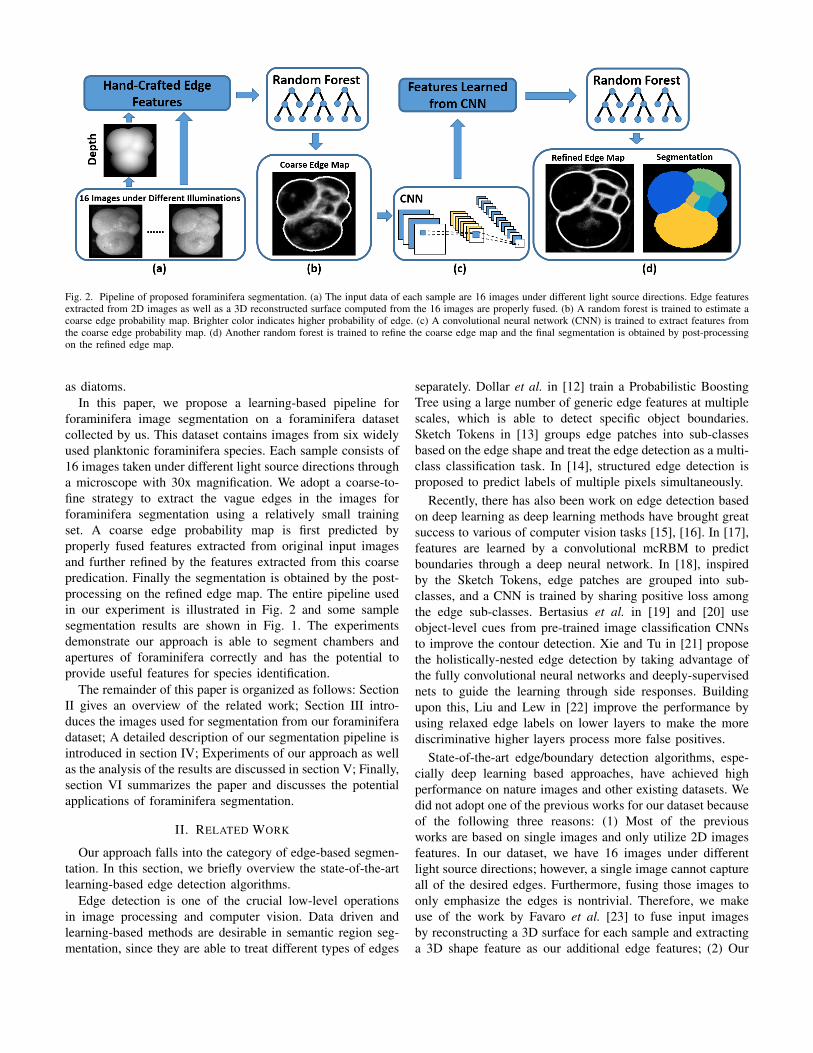
Fig. 2. Pipeline of proposed foraminifera segmentation. (a) The input data of each sample are 16 images under different light source directions. Edge featuresextracted from 2D images as well as a 3D reconstructed surface computed from the 16 images are properly fused. (b) A random forest is trained to estimate acoarse edge probability map. Brighter color indicates higher probability of edge. (c) A convolutional neural network (CNN) is trained to extract features fromthe coarse edge probability map. (d) Another random forest is trained to refine the coarse edge map and the final segmentation is obtained by post-processingon the refined edge map.

as diatoms.In this paper, we propose a learning-based pipeline for

foraminifera image segmentation on a foraminifera datasetcollected by us. This dataset contains images from six widelyused planktonic foraminifera species. Each sample consists of16 images taken under different light source directions througha microscope with 30x magnification. We adopt a coarse-to-fine strategy to extract the vague edges in the images forforaminifera segmentation using a relatively small trainingset. A coarse edge probability map is first predicted byproperly fused features extracted from original input imagesand further refined by the features extracted from this coarsepredication. Finally the segmentation is obtained by the post-processing on the refined edge map. The entire pipeline usedin our experiment is illustrated in Fig. 2 and some samplesegmentation results are shown in Fig. 1. The experimentsdemonstrate our approach is able to segment chambers andapertures of foraminifera correctly and has the potential toprovide useful features for species identification.

The remainder of this paper is organized as follows: SectionII gives an overview of the related work; Section III intro-duces the images used for segmentation from our foraminiferadataset; A detailed description of our segmentation pipeline isintroduced in section IV; Experiments of our approach as wellas the analysis of the results are discussed in section V; Finally,section VI summarizes the paper and discusses the potentialapplications of foraminifera segmentation.

II. RELATED WORK

Our approach falls into the category of edge-based segmen-tation. In this section, we briefly overview the state-of-the-artlearning-based edge detection algorithms.

Edge detection is one of the crucial low-level operationsin image processing and computer vision. Data driven andlearning-based methods are desirable in semantic region seg-mentation, since they are able to treat different types of edges

separately. Dollar et al. in [12] train a Probabilistic BoostingTree using a large number of generic edge features at multiplescales, which is able to detect specific object boundaries.Sketch Tokens in [13] groups edge patches into sub-classesbased on the edge shape and treat the edge detection as a multi-class classification task. In [14], structured edge detection isproposed to predict labels of multiple pixels simultaneously.

Recently, there has also been work on edge detection basedon deep learning as deep learning methods have brought greatsuccess to various of computer vision tasks [15], [16]. In [17],features are learned by a convolutional mcRBM to predictboundaries through a deep neural network. In [18], inspiredby the Sketch Tokens, edge patches are grouped into sub-classes, and a CNN is trained by sharing positive loss amongthe edge sub-classes. Bertasius et al. in [19] and [20] useobject-level cues from pre-trained image classification CNNsto improve the contour detection. Xie and Tu in [21] proposethe holistically-nested edge detection by taking advantage ofthe fully convolutional neural networks and deeply-supervisednets to guide the learning through side responses. Buildingupon this, Liu and Lew in [22] improve the performance byusing relaxed edge labels on lower layers to make the morediscriminative higher layers process more false positives.

State-of-the-art edge/boundary detection algorithms, espe-cially deep learning based approaches, have achieved highperformance on nature images and other existing datasets. Wedid not adopt one of the previous works for our dataset becauseof the following three reasons: (1) Most of the previousworks are based on single images and only utilize 2D imagesfeatures. In our dataset, we have 16 images under differentlight source directions; however, a single image cannot captureall of the desired edges. Furthermore, fusing those images toonly emphasize the edges is nontrivial. Therefore, we makeuse of the work by Favaro et al. [23] to fuse input imagesby reconstructing a 3D surface for each sample and extractinga 3D shape feature as our additional edge features; (2) Our

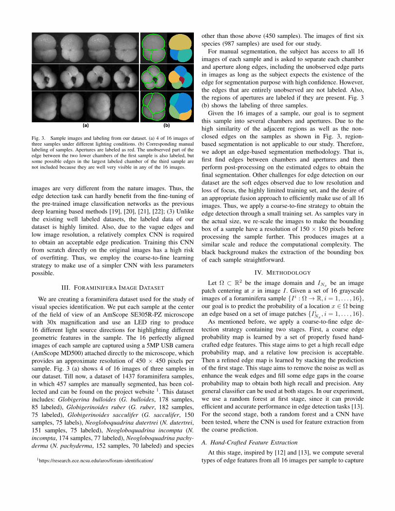
Fig. 3. Sample images and labeling from our dataset. (a) 4 of 16 images ofthree samples under different lighting conditions. (b) Corresponding manuallabeling of samples. Apertures are labeled as red. The unobserved part of theedge between the two lower chambers of the first sample is also labeled, butsome possible edges in the largest labeled chamber of the third sample arenot included because they are well very visible in any of the 16 images.

images are very different from the nature images. Thus, theedge detection task can hardly benefit from the fine-tuning ofthe pre-trained image classification networks as the previousdeep learning based methods [19], [20], [21], [22]; (3) Unlikethe existing well labeled datasets, the labeled data of ourdataset is highly limited. Also, due to the vague edges andlow image resolution, a relatively complex CNN is requiredto obtain an acceptable edge predication. Training this CNNfrom scratch directly on the original images has a high riskof overfitting. Thus, we employ the coarse-to-fine learningstrategy to make use of a simpler CNN with less parameterspossible.

III. FORAMINIFERA IMAGE DATASET

We are creating a foraminifera dataset used for the study ofvisual species identification. We put each sample at the centerof the field of view of an AmScope SE305R-PZ microscopewith 30x magnification and use an LED ring to produce16 different light source directions for highlighting differentgeometric features in the sample. The 16 perfectly alignedimages of each sample are captured using a 5MP USB camera(AmScope MD500) attached directly to the microscope, whichprovides an approximate resolution of 450 × 450 pixels persample. Fig. 3 (a) shows 4 of 16 images of three samples inour dataset. Till now, a dataset of 1437 foraminifera samples,in which 457 samples are manually segmented, has been col-lected and can be found on the project website 1. This datasetincludes: Globigerina bulloides (G. bulloides, 178 samples,85 labeled), Globigerinoides ruber (G. ruber, 182 samples,75 labeled), Globigerinoides sacculifer (G. sacculifer, 150samples, 75 labels), Neogloboquadrina dutertrei (N. dutertrei,151 samples, 75 labeled), Neogloboquadrina incompta (N.incompta, 174 samples, 77 labeled), Neogloboquadrina pachy-derma (N. pachyderma, 152 samples, 70 labeled) and species

1https://research.ece.ncsu.edu/aros/foram-identification/

other than those above (450 samples). The images of first sixspecies (987 samples) are used for our study.

For manual segmentation, the subject has access to all 16images of each sample and is asked to separate each chamberand aperture along edges, including the unobserved edge partsin images as long as the subject expects the existence of theedge for segmentation purpose with high confidence. However,the edges that are entirely unobserved are not labeled. Also,the regions of apertures are labeled if they are present. Fig. 3(b) shows the labeling of three samples.

Given the 16 images of a sample, our goal is to segmentthis sample into several chambers and apertures. Due to thehigh similarity of the adjacent regions as well as the non-closed edges on the samples as shown in Fig. 3, region-based segmentation is not applicable to our study. Therefore,we adopt an edge-based segmentation methodology. That is,first find edges between chambers and apertures and thenperform post-processing on the estimated edges to obtain thefinal segmentation. Other challenges for edge detection on ourdataset are the soft edges observed due to low resolution andloss of focus, the highly limited training set, and the desire ofan appropriate fusion approach to efficiently make use of all 16images. Thus, we apply a coarse-to-fine strategy to obtain theedge detection through a small training set. As samples vary inthe actual size, we re-scale the images to make the boundingbox of a sample have a resolution of 150 × 150 pixels beforeprocessing the sample further. This produces images at asimilar scale and reduce the computational complexity. Theblack background makes the extraction of the bounding boxof each sample straightforward.

IV. METHODOLOGY

Let Ω ⊂ R2 be the image domain and INxbe an image

patch centering at x in image I . Given a set of 16 grayscaleimages of a foraminifera sample Ii : Ω→ R, i = 1, . . . , 16,our goal is to predict the probability of a location x ∈ Ω beingan edge based on a set of image patches IiNx

, i = 1, . . . , 16.As mentioned before, we apply a coarse-to-fine edge de-

tection strategy containing two stages. First, a coarse edgeprobability map is learned by a set of properly fused hand-crafted edge features. This stage aims to get a high recall edgeprobability map, and a relative low precision is acceptable.Then a refined edge map is learned by stacking the predictionof the first stage. This stage aims to remove the noise as well asenhance the weak edges and fill some edge gaps in the coarseprobability map to obtain both high recall and precision. Anygeneral classifier can be used at both stages. In our experiment,we use a random forest at first stage, since it can provideefficient and accurate performance in edge detection tasks [13].For the second stage, both a random forest and a CNN havebeen tested, where the CNN is used for feature extraction fromthe coarse prediction.

A. Hand-Crafted Feature Extraction

At this stage, inspired by [12] and [13], we compute severaltypes of edge features from all 16 images per sample to capture

Fig. 4. Selected hand-crafted features of the second sample in Fig. 3. (a)Standard deviation image. (b) Depth map of reconstructed 3D surface. (c)Curvature map. This map captures all the edges of chambers but can hardlycapture the aperture edges. (d) and (e) Two ridge maps computed from 2 of16 images. Part of the aperture boundary is not captured in (d) but capturedin (e). (f) Maximum of 16 ridge maps.

the edge cues in various aspects. We employ both genericedge features and a 3D shape feature computed from a re-constructed 3D surface of the sample.

The generic edge features used in our experiment includegradient, difference of Gaussian (DoG), and ridge detector.The gradient magnitudes are computed per image using Gaus-sian kernels with σ = 0.8 and 2. In addition, we split thegradients into four directions, θ = 0, π/4, π/2 and 3π/4,to compute 4 more gradient maps per image at each scale.Two DoG maps are computed from the difference of threeGaussian blurs with σ = 2.5, 4 and 6.4 per image. Ridgepoints are defined as the maximum or minimum points inthe main principal curvature of an image function [24]. Theridge detector is adopted due to the presence of some thickedges on samples that resemble ridges or valleys of the imagefunction, which produce double low magnitude lines whenapplying edge detectors. Because most of the edges have colorintensities lower than the chambers, we only use the ridgedetector to highlight the valley in the images. The detectorhas the form

L =1

2(Fxx + Fyy −

√(Fxx − Fyy)2 + 4F 2

xy), (1)

where Fxx, Fyy and Fxy are the second derivatives of theimage I in the gradient direction x, y and xy, respectively.We compute one ridge map per image using a Gaussian filterwith σ = 3.2. Fig. 4 (d) and (e) show examples of the ridgemaps.

As the entire set of edges can hardly be captured in asingle image, simply concatenating features of all the inputimages may introduce noise and is computationally inefficientas well. However, all the edge information in the imagescan be collected by maximizing the edge cues over the 16images. Since the images are perfectly aligned, the fusedfeature maps can be obtained by taking the maximum featurevalue at each pixel location over the 16 images. We do notutilize quantiles for feature fusion to get rid of some noiseoccasionally shown in the images because it may remove someweak desirable edges as well, which leads to a lower recall.After the aggregating, the number of feature maps reducesfrom 208 to 13.

As we can see in Fig. 3, some edges have small variationsunder different light sources, the standard deviation at eachpixel location over 16 images can provide relatively rich edgeinformation (An example of this is shown in Fig. 4 (a)).

Therefore we compute a DoG of the standard deviation imageusing σ = 3.2 and 5.1 as an additional feature map.

To make use of the 16 images which highlight the differ-ent geometric features of the sample, we apply an efficientuncalibrated photometric stereo technique [23] to reconstructa 3D surface of each sample for better fusion of the inputimages, followed by a Bilateral filter [25] with σ = 0.1 toremove the small variations on the chambers. A sample depthmap of a reconstructed 3D surface is shown in Fig. 4 (b). Thenoise introduced by color changes and textures on the samplesis removed, since they do not have large changes in depth.Also, edges between chambers are captured well in the depthmap. We compute the maximum normal curvature [26] of thisreconstructed surface as another feature map. This feature mapmeasures the maximum bending at each point of the surfaceand is computed by

κ = H +√H2 −K, (2)

where H is the mean curvature and K is the Gaussiancurvature of the surface. Please refer to [26] for more details.Fig. 4 (c) shows an example curvature map.

In summary, we have 15 maps per sample, consisting of10 gradient maps, 3 DoG maps, 1 ridge map, and 1 curvaturemap. Each pixel location is represented by a 3375 dimensionalfeature vector, obtained by centering a 15× 15 patch on thatpixel and concatenating the features obtained from each of the15 feature maps.

B. Coarse Edge Probability Map Prediction

We use a random forest to predict the coarse edge prob-ability map. A random forest is an ensemble of randomlytrained decision trees and the output is the average predictionof individual trees [27]. Since boundaries of foraminifera andapertures are comparatively sharper than the edges betweenchambers, these two types of edges are divided into two classesto increase the training efficiency as well as to distinguishbetween apertures and chambers for segmentation. Afterwards,the coarse edge probability map is predicted by a 3-classclassification random forest.

Fig. 7 (c) and (d) show some coarse edge probability mapsestimated at this stage. Though the recall of the observeddesired edges is high, due to the outcomes of max poolingduring feature extraction, the estimated edges are thick, andedges observed in the texture (but not corresponding to realchamber boundaries) are also detected in the probability map.Besides the reason that some edges on the samples are narrowregions rather than thin lines, Fig. 4 illustrates another reasonarises the thick predicted edges. The shade of the edgevaries slightly under different light source directions, whichintroduces small offsets to the edge features over 16 images.Thus, the edge in the fused feature map is a thick region ratherthan a thin line. Other undesired patterns of the coarse edgemaps are the low probabilities of some edges and non-closedboundaries due to the weak edges or the unobserved edges inthe images. To obtain higher precision edge maps, a secondstage for refinement is necessary.

Fig. 5. Hand-crafted features and deep features computed from a coarseedge probability map. (a) Top: One of original sample images. Bottom:Corresponding coarse edge probability map. The unclear edges in the originalimages get low probability (marked with a red box). There is also some noisedue to the texture on the chambers. (b) Top row: Four hand-crafted edgefeatures of the coarse edge map, including two gradient magnitude mapsand two DoG maps. Bottom row: Four sample deep feature maps. In thehand-crafted feature maps, especially for the first two, the weak edges of thecoarse map have almost the same patterns as the noise on the upper and rightchambers; however, in deep feature maps, the weak edges are shown muchclearly with patterns far different from the noise, which makes the classifierdistinguish weak edges from noise more easily. Best viewed in color.

C. Refinement of Coarse Edge Probability Map

At this stage, we further refine the coarse edge probabilitymap to obtain a high precision by thinning the edges, removingnoise, enhancing the probability of desired edges and closingas many boundaries as possible. From Fig. 7 (d), we cantell the location of chamber and aperture edges purely basedon the noisy coarse edge map. But those edges cannot beextracted automatically with a high accuracy through a simpleprocess, like thresholding. Therefore, we apply a learning-based approach at this stage and only the predicted coarseedge map is used as input. Similar to the previous stage,features are first extracted from the coarse map and each pixelis represented by a small patch centered around it. Then theedge map is refined through another classifier. Two types offeatures have been tried in our experiment: hand-crafted edgefeatures and deep features learned by a CNN trained for edgemap refinement. Both approaches are discussed in detail inthis section. We start from the hand-crafted feature extraction.

1) Hand-Crafted Features: Since the edge location in theprobability map is much clearer than in the original 16images, a smaller number of features need to be extractedfrom the probability map. This reduced feature set includesgradient and DoG with the same parameters as computedfrom the original images at the first stage. In summery, 12feature maps are computed and a patch size 15 × 15 givesa 2700 dimensional feature vector for each pixel location.Because the classification of aperture boundaries at the firststage is accurate enough for aperture region segmentation andall types of edges have similar patterns in the input coarseprobability map, pixels are labeled as two classes: edge andnon-edge. Next, the refined edge map is obtained by traininga classification random forest again. Fig. 7 (e) shows someresults of the refined edge map. The edge probability map ismuch clearer than before and the weak edges are enhanced as

well. Also, some non-closed boundaries are closed, becausethe training data contains some examples of filling edge gaps,which makes the classifier have the ability to hallucinate edgesby fusing features in the patch as discussed in [12]. Betterboundary completion performance can be achieved throughcareful selection of training data and use of larger patches.

2) Deep Features: The features we extract for refinementin section IV-C are purely edge detectors. However, there mayexist better features to remove noise as well as enhance thelow confidence edges in the coarse map. To investigate this,we employ a CNN to learn a set of features automaticallyfrom the coarse probability map.

A CNN consists of one or more convolutional layers fol-lowed by one or more fully connected layers. It often containsa pooling layer between two convolutional layers to reducecomplexity [28]. In our experiment, we use four convolutionallayers and two fully connected layers as used in [18], whichis sufficient for low-level feature extraction as suggested in[18]. The only difference is that we do not use local responsenormalization layers (LRN). The input of this CNN is a 32×32patch of coarse probability map and it is trained to label thecenter point of each patch as edge or non-edge. Dropout [29]with probability 0.5 is used in the first fully connected layer(FC1) during training to reduce the risk of overfitting.

Similar to [18], we use the output of FC1 (a 128-dimensional feature vector) as our deep features of each pixeland thus we can show the feature maps in the same way asin [18]. The comparison of hand-crafted features and deepfeatures can be found in Fig. 5. Both weak and strong edgesin the coarse edge map are more distinguishable from noisein deep feature maps, which makes the noise suppressionand edge enhancement much easier through a classifier. Weconcatenate the features of all the pixels in a 11 × 11 patchto obtain a 15488-dimensional feature vector to represent thecentering pixel. Again, a random forest is trained using thedeep features for the edge probability map refinement. Fig.7 (f) shows some sample results. The refined edge maps arecomparable to those refined by hand-crafted features, but aremore accurate for some small details and also get more closedboundaries because of the more powerful features.

Fig. 6 explains how the edge detection improves by usingthe coarse-to-fine strategy. At the first stage, only a set ofsmall patches is used to predict each pixel location. Thoughthe prediction is noisy, the edge information is clearer thanthe original input. Every time we go to the next stage, wecan efficiently gather the information from larger patches inoriginal images by taking small patches in the prediction ofthis stage and obtaining an even clearer predication. If deepfeatures are employed, each pixel in the final predication isbased on a set of 57 × 57 patches in the original images.This is similar to the image processing through a CNN,which indicates the possibility of using an end-to-end learningprocess through a CNN. However, instead of learning featuresfrom original images directly, we use hand-crafted featuresat the first stage followed by a relatively simple CNN. Thisprocedure largely reduces the risk of overfitting due to the

Fig. 6. Data flow of our coarse-to-fine edge detection using deep features.Paths with different colors illustrate computation patch of a pixel location atdifferent stages. (a) Input 16 sample images. (b) Each pixel in the coarse edgemap is predicted by a set of 15×15 patches in original images. (c) Each pixelin the deep feature maps is computed by a 32×32 patches in the coarse edgemap and thus depending on a set of 46×46 patches in the original images. (d)Each pixel location in the refined edge map is predicted by a set of 11× 11patches in deep feature maps and then depending on a 43× 43 patch in thecoarse edge map. Thus each pixel in the final refined edge map is predictedbased on the information gathering from a set of 57 × 57 patches from theoriginal images.

highly limited training data.

D. Post-Processing

To further close the boundaries, a closing operation using adisk with radius of 2 is applied to the refined edge probabilitymap after thresholding. Afterwards, the final segmentation isobtained by growing the regions separated by those edgesbased on distance. If aperture edges are detected in the coarseprobability map, then a region in the image that is overlappingwith the aperture edge is labeled as an aperture given thatits average color intensity (over all 16 images) is considereddark enough. We check this by comparing the color againsta two group k-means clustering performed using the trainingdata. The clustering using the training data is repeated 5 timesin order to gain robustness, and a test region is labeled asaperture only if falls in the appropriate cluster more than50% of the time (i.e., 3 times in this case). Fig. 7 (g) showssome final segmentation results. The edge thinning by regiongrowing removes some non-closed boundaries but it also getsrid of the small branches that could be produced throughskeletonization.

V. EXPERIMENT

In this section, we evaluate our foraminifera edge detectionand segmentation qualitatively and quantitatively.

A. Implementation Details

We randomly choose 100 samples from the 457 labeledsamples as our training samples: 25 are used to train the firststage, and 75 for the second stage. That leaves 357 labeledand 530 unlabeled samples for testing. The training edges arethickened by 6 pixel at the first stage and by 4 pixels at thesecond stage.

For the first stage, 62.5k non-edge patches (2.5k per sam-ple), 37k chamber edge patches (all chamber edges in 25samples) and 50k other edge patches (2k per sample) arerandomly sampled as the training set. At the second stage,the random forest using hand-crafted features is trained byrandomly sampling 96k positive patches (all edges in 75

samples) and 150k negative patches (2k per sample) from the75 samples. To train the deep features, the patches from the 75samples are divided into a set of 17k validation data points (7kpositive and 10k negative) from 5 samples and a set of 229ktraining data points (89k positive and 140k negative) from70 samples. Then a random forest using the deep features istrained by randomly sampling 37.5K positive patches (500 persamples) and 60k (800 per sample) negative patches from the75 samples.

The random forests parameters used in our experiment areall the same. Each random forest is trained until all the leafnodes only contain one class using a collection of 150 trees,except for the one trained using deep features which consistsof 50 trees to reduce the time consumption. The CNN forlearning deep feature is trained using 200 epochs with batchsize 5000. The learning rate for the first 100 epochs is 0.01and set to 0.001 for the remaining 100 epochs.

The random forests are implemented in MATLAB andthe CNN is implemented in Python using the Tensorflowframework [30]. The experimental environment is CPU i7 with64GB RAM and NVIDIA TITAN GPU. For a sample imagewith resolution 166 × 166, computing one coarse edge mapneeds 24 seconds. Refinement through hand-crafted featuresrequires 18 seconds and through deep features requires about100 seconds (1 minutes for feature extraction and 40 secondsfor edge patch classification). Note that these steps can belargely optimized through implementation of a fully convolu-tional network and parallel computing.

B. Qualitative and Quantitative Evaluation

Results of each stage of our approach are shown in Fig.7. Coarse edge probability maps (RF) obtained at the firststage are able to collect most of the edge clues from the inputimage set, but some edges are thick or detected with low con-fidence, which causes some non-closed boundaries. However,the aperture boundaries and chamber edges are separated wellat this stage (RF label). At the second stage, hand-craftedfeatures (RF+RF(HF)) and deep features (RF+RF(DF)) givesimilar performance; however, deep features provide higherconfidence for weak edges, more accurate details and moreclosed boundaries. Also, as shown in the last row of Fig.7, if the edges in the input images are too weak to getcaptured at the first stage, they will not be detected by therefinement either. Another observation is that the machinesegmentation can be better than manually labeling in somecases. Edges unclear to humans are located by efficientlycollecting information from a neighborhood of each pixel.

To quantitatively demonstrate the improvement of the sec-ond stage and evaluate the performance, we use three edgedetection evaluation metrics: the best F-measure for a fixedthreshold (ODS), the average F-measure of the best thresholdfor each image (OIS) and the average precision over allthreshold (AP), as well as three segmentation metrics: the bestweighted covering score (W), un-weighted covering score (Un-W) [31] and recall of regions (Recall) for fixed thresholds.The edge recall is defined as the percentage of the labeling

Fig. 7. Sample results of different species. Sample images (a), manuallabeling (b), edge labeling after first stage (c), edge probabilities from variousapproaches (d)-(f), and final segmentation using deep features (g) are shown.For the first stage (c), edges between chambers are labeled in green and otheredges are yellow. Aperture is labeled as red in segmentation (g). Window W1shows an example in which correct machine labeling and human labeling canhave some offsets. Window W2 shows how deep features can close non-closedboundaries in the refined map. Window W3 illustrates an example in whichmachine labeling can be better than human labeling. Window W4 shows howthe refined map (stage 2) can enhance weak edges as well as remove noisefrom the coarse map. The last row shows a failed example due to edges thatare too vague to be captured in the coarse map.

Fig. 8. Additional results. (a) Using patch size 57 × 57 for random forest.(b) Using deep features computed by a CNN from a 16-channel image.

edges covered by the thresholding estimated edge map. Theedge precision is defined as the percentage of the estimatededge pixels covering the labeling edges. The labeling edges arethickened to 8 pixels wide for precision computation since theactual edges between chambers can be narrow regions, whichgenerate thick estimated edges and small offsets betweenhuman labeling and the correctly estimated edges. For seg-mentation evaluation, weighted covering score is the averagecovering score weighted by the area of each region in humanlabeling. We also use un-weighted covering score becausefor species identification purpose, every chamber and aperturehave equal importance. To evaluate how well the chambers andapertures are detected, we define the recall of regions for eachsample as the percentage of the labeling regions detected inthe estimated segmentation, where each region in the humanlabeling is regarded as detected if there exists an overlappingestimated region with covering ratio greater than 0.5.

Table I presents the scores at each stage. The precision

TABLE IEDGE DETECTION RESULTS USING DIFFERENT FEATURES AND

CLASSIFIERS

Edge RegionODS OIS AP W Un-W Recall

RF .841 .853 .698 .779 .645 .695RF+RF(HC) .867 .875 .775 .825 .715 .779RF+RF(DF) .872 .879 .771 .821 .721 .786RF(2D) .842 .852 .691 .757 .616 .659RF(100) .841 .853 .650 .803 .678 .753RF+RF(HC43) .868 .877 .759 .821 .713 .764

is relatively low compared with other metrics even with thethickened labeling because of the thick estimated edges andthe inaccurate of human labeling as shown in Fig. 7. But wedo observe the improvement of precision after the refinement.Besides this, we can see a large performance gain from the firststage (RF) to the second stage (RF+RF(HC) and RF+RF(DF)),especially for region scores. The closing of boundaries onlybrings small changes in the sense of edge, but can highlyincrease the segmentation accuracy. The increase of averageprecision also suggest the thin edges in refined edge maps.Deep features (RF+RF(DF)) refinement is slightly better thanhand-crafted features (RF+RF(HC)). The higher un-weightedcovering and region recall scores indicate that deep featuresare more capable in detecting small regions, most of which areapertures. Thus, deep features are preferred for the applicationsin which aperture detection is crucial. Otherwise, hand-craftedfeatures, which are good enough to correctly segment most ofthe chambers, can be used for computational efficiency.

We also report scores of the first stage without 3D fea-tures (RF(2D)), the decrease in the region scores of (RF)demonstrates 3D features can enhance some weak edges toclose more boundaries. To be comparable with deep features(RF+RF(DF)), which gather information from 43×43 patchesin the coarse map, we report the scores of refinement withhand-crafted features using 43 × 43 patch (RF+RF(HC43)).The similar scores with 15 × 15 patch size indicate that thebetter performance in small details cannot be achieved by sim-ply increasing the patch size. To show that the improvementof the second stage is not purely because of the increasingof the training set, the scores of the first stage with all 100training samples (RF(100)) are reported. It hardly improves theedge detection performance, but improves the segmentation byproviding higher detection confidence for some weak edges.Still, it cannot beat the performance of using a second stagefor refinement.

We have also tried other two settings with only one stageusing 100 training sample images: using patch size 57×57 fora random forest to compare with deep features, and extractingdeep features directly from a 16-channel image formed fromthe original images using a CNN with the same architectureas used in our experiment. Results of these two settings areshown in Fig. 8. The outputs do not have the same qualityas the two stage refinement process, which is able to gatherinformation more efficiently and requires a less complex CNN.

VI. CONCLUSION

In this paper, we propose a coarse-to-fine edge detectionapproach on our foraminifera dataset. We use a two-stagestrategy to achieve accurate edge detection and segmentationperformance using a relatively small training data throughadditional 3D features and features learned from a CNN.The experiments demonstrate that the machine segmentationis able to correctly label chambers and apertures on samples.There are several applications for the segmentation results.Sample images of specific species can be selected by searchingamong the segmentation results. For example, one can getimages of G. bulloides by picking the samples with oneaperture and four chambers in the segmentation results. Also,by representing regions as nodes in a graph and connectingthe nodes of adjacent regions, we can construct a graph torepresent the structure of each sample. General structures ofdifferent species can be learned from a training set and speciescan be identified through graph matching. Additionally, theactual size of chambers and apertures can be computed tohelp with the morphological study of the shells.

ACKNOWLEDGMENT

We thank Svapnil Ankolkar, Mehdi Garcia Cornell, BryantDelgado and Sadaf Iqbal for the help on image capturing andJason Farsaie for him help on image labeling. This work wassupported by the National Science Foundation under awardOCE-1637039.

REFERENCES

[1] B. K. B. K. Sen Gupta, Modern foraminifera. Dordrecht ; Boston :Kluwer Academic Publishers, 1999, includes bibliographical references(p. 299-351) and indexes.

[2] K. Vickerman, “The diversity and ecological significance of protozoa,”Biodiversity & Conservation, vol. 1, no. 4, pp. 334–341, 1992.

[3] J. M. Bernhard and B. K. Sen Gupta, Foraminifera of oxygen-depletedenvironments. Dordrecht: Springer Netherlands, 2003, pp. 201–216.

[4] J. A. Cushman and A. C. Ellisor, “The foraminiferal fauna of the anahuacformation,” Journal of Paleontology, vol. 19, no. 6, pp. 545–572, 1945.

[5] W. A. Berggren, “Ecology and palaeoecology of benthic foraminifera.”The Journal of Protozoology, vol. 39, no. 4, pp. 537–537, 1992.

[6] W. A. BERGGREN, “A cenozoic time-scale some implications forregional geology and paleobiogeography,” Lethaia, vol. 5, no. 2, pp.195–215, 1972.

[7] S. Liu, M. Thonnat, and M. Berthod, “Automatic classification ofplanktonic foraminifera by a knowledge-based system,” in Proceedingsof the Tenth Conference on Artificial Intelligence for Applications, Mar1994, pp. 358–364.

[8] J. Kennett and M. Srinivasan, Neogene planktonic foraminifera: aphylogenetic atlas. Hutchinson Ross, 1983.

[9] R. Marmo and S. Amodio, A Neural Network for Classification ofChambers Arrangement in Foraminifera. Berlin, Heidelberg: SpringerBerlin Heidelberg, 2006, pp. 271–278.

[10] B. H. Corliss, “Morphology and microhabitat preferences of benthicforaminifera from the northwest atlantic ocean,” Marine micropaleon-tology, vol. 17, no. 3-4, pp. 195–236, 1991.

[11] E. Boltovskoy, D. B. Scott, and F. Medioli, “Morphological variationsof benthic foraminiferal tests in response to changes in ecologicalparameters: a review,” Journal of Paleontology, vol. 65, no. 02, pp. 175–185, 1991.

[12] P. Dollar, Z. Tu, and S. Belongie, “Supervised learning of edges andobject boundaries,” in 2006 IEEE Computer Society Conference onComputer Vision and Pattern Recognition (CVPR’06), vol. 2, 2006, pp.1964–1971.

[13] J. J. Lim, C. L. Zitnick, and P. Dollr, “Sketch tokens: A learned mid-level representation for contour and object detection,” in 2013 IEEEConference on Computer Vision and Pattern Recognition, June 2013,pp. 3158–3165.

[14] P. Dollr and C. L. Zitnick, “Fast edge detection using structured forests,”IEEE Transactions on Pattern Analysis and Machine Intelligence,vol. 37, no. 8, pp. 1558–1570, Aug 2015.

[15] A. Krizhevsky, I. Sutskever, and G. E. Hinton, “Imagenet classificationwith deep convolutional neural networks,” in Proceedings of the 25thInternational Conference on Neural Information Processing Systems.Curran Associates Inc., 2012, pp. 1097–1105.

[16] R. Girshick, J. Donahue, T. Darrell, and J. Malik, “Rich featurehierarchies for accurate object detection and semantic segmentation,”in 2014 IEEE Conference on Computer Vision and Pattern Recognition,June 2014, pp. 580–587.

[17] J. J. Kivinen, C. K. I. Williams, and N. Heess, “Visual boundaryprediction: A deep neural prediction network and quality dissection,”in AISTATS, 2014.

[18] W. Shen, X. Wang, Y. Wang, X. Bai, and Z. Zhang, “Deepcontour: Adeep convolutional feature learned by positive-sharing loss for contourdetection,” in 2015 IEEE Conference on Computer Vision and PatternRecognition (CVPR), June 2015, pp. 3982–3991.

[19] G. Bertasius, J. Shi, and L. Torresani, “Deepedge: A multi-scale bi-furcated deep network for top-down contour detection,” in 2015 IEEEConference on Computer Vision and Pattern Recognition (CVPR), June2015, pp. 4380–4389.

[20] ——, “High-for-low and low-for-high: Efficient boundary detection fromdeep object features and its applications to high-level vision,” in 2015IEEE International Conference on Computer Vision (ICCV), Dec 2015,pp. 504–512.

[21] S. Xie and Z. Tu, “Holistically-nested edge detection,” in 2015 IEEEInternational Conference on Computer Vision (ICCV), Dec 2015, pp.1395–1403.

[22] Y. Liu and M. S. Lew, “Learning relaxed deep supervision for better edgedetection,” in 2016 IEEE Conference on Computer Vision and PatternRecognition (CVPR), June 2016, pp. 231–240.

[23] P. Favaro and T. Papadhimitri, “A closed-form solution to uncalibratedphotometric stereo via diffuse maxima,” in 2012 IEEE Conference onComputer Vision and Pattern Recognition, June 2012, pp. 821–828.

[24] T. Lindeberg, “Edge detection and ridge detection with automatic scaleselection,” International Journal of Computer Vision, vol. 30, no. 2, pp.117–156, Nov 1998.

[25] C. Tomasi and R. Manduchi, “Bilateral filtering for gray and colorimages,” in Sixth International Conference on Computer Vision (IEEECat. No.98CH36271), Jan 1998, pp. 839–846.

[26] R. Goldman, “Curvature formulas for implicit curves and surfaces,”Comput. Aided Geom. Des., vol. 22, no. 7, pp. 632–658, Oct. 2005.

[27] A. Criminisi, E. Konukoglu, and J. Shotton, “Decision forestsfor classification, regression, density estimation, manifold learningand semi-supervised learning,” Tech. Rep., October 2011. [Online].Available: https://www.microsoft.com/en-us/research/publication/decision-forests-for-classification-regression-density-estimation-manifold-learning-and-semi-supervised-learning/

[28] I. Goodfellow, Y. Bengio, and A. Courville, Deep Learning. MIT Press,2016, http://www.deeplearningbook.org.

[29] N. Srivastava, G. Hinton, A. Krizhevsky, I. Sutskever, and R. Salakhut-dinov, “Dropout: A simple way to prevent neural networks from over-fitting,” J. Mach. Learn. Res., vol. 15, no. 1, pp. 1929–1958, Jan. 2014.

[30] M. Abadi, A. Agarwal, P. Barham, E. Brevdo, Z. Chen, C. Citro, G. S.Corrado, A. Davis, J. Dean, M. Devin, S. Ghemawat, I. Goodfellow,A. Harp, G. Irving, M. Isard, Y. Jia, R. Jozefowicz, L. Kaiser,M. Kudlur, J. Levenberg, D. Mane, R. Monga, S. Moore, D. Murray,C. Olah, M. Schuster, J. Shlens, B. Steiner, I. Sutskever, K. Talwar,P. Tucker, V. Vanhoucke, V. Vasudevan, F. Viegas, O. Vinyals,P. Warden, M. Wattenberg, M. Wicke, Y. Yu, and X. Zheng,“TensorFlow: Large-scale machine learning on heterogeneous systems,”2015, software available from tensorflow.org. [Online]. Available:http://tensorflow.org/

[31] P. Arbelaez, M. Maire, C. Fowlkes, and J. Malik, “Contour detectionand hierarchical image segmentation,” IEEE Transactions on PatternAnalysis and Machine Intelligence, vol. 33, no. 5, pp. 898–916, May2011.