Coalition list (or of lists): does it matter for …scal

policies? Evidence from Italy.

Leonzio Rizzo (Università di Ferrara & IEB)

and Alberto Zanardi (Università di Bologna & Econpubblica-Università Bocconi)

October 25, 2011

Abstract

he aim of this paper is to empirically test with data on all Italian municipalities from2001-2006 to what extent two electoral rules, holding in Italy for municipality dependingon their population level with respect to the 15,000 inhabitants threshold a¤ect …scalpolicies decisions. Municipalities with less than 15,000 inhabitants elect the mayor byadopting a single ballot plurality rule where only a single list can support the candidate;municipalities with more than 15,000 inhabitants elect the mayor by adopting a run-o¤plurality rule, not imposing any restriction on the number of lists that can support amayoral candidate and also enabling the aggregation (between the …rst and second roundin the case of a second ballot) of new lists in support of one or other of the candidatesstill in the race. Moreover, in the latter case the majority premium to the coalition isgiven only if it passed a vote-threshold of 40 percent ; this contrasts the absence of bindingconstraints to get the majority premium of 66 percent in the electoral regime for the smallmunicipalities. The large-municipality electoral system generates more lists heterogeneityin power than the small-municipality-electoral system and typical common pool problemscan make …nancial targets very hard to be maintained successfully than in the case a strongmayor supported by his own list is in power. We …nd evidence that a large municipalitywith respect to a small one, decreases direct taxes but no e¤ect on expenditure is found.This contrasts with previous …nding (Roubini and Sachs, 1989; Kontopoulos and Perotti,1999) where the free-riding problem generate a higher level expenditure …nanced througha de…cit increase. This is due to the very strict …nancial rule of the municipalities whichare basically not allowed to run any de…cit, but can play with their surplus devoted to…nance future investments.

JEL codes: H3, H21, H77keywords: federal budget, double ballot, coaltion, list, taxes, expenditures.

1

1 Introduction1

Electoral systems play a crucial role in shaping electoral incentives within which public policies

are established. The political economy literature has devoted a lot of work in exploring the

impact on public expenditure of plurality versus proportional electoral rules and districts size

(Austen-Smith, 2000; Lizzeri and Persico, 2001; Mayerson, 1993; Persson and Tabellini, 2000).

Almost no attention, except for a recent work by Bordignon Nannicini and Tabellini (2010),

has been given to the possibility that the election takes place not in a one shot game, but in

a two-stage game as in some electoral system happens: this is the so-called double ballot (or

run-o¤) system. Broadly speaking, voters in the …rst round select a subset of candidates, over

which they vote again in the second round. The best known example of this system is that

one used in France for the Presidential election, where the two candidates getting more votes

in the …rst ballot go for a second …nal round. Other examples are in Latin America, in US for

the gubernatorial elections and in Italy for the elections of the mayor in municipalities.

We focus our attention on the Italian case. This is very interesting for studying the impact

on …scal policies, in fact the system for municipalities with more than 15,000 inhabitans does

not impose any restriction on the number of lists that can support a mayoral candidate, it also

enables the aggregation, between the …rst and second round in the case of a second ballot, of

new lists in support of one or other of the candidates still in the race. On the contrary, only

one list can support the mayor in the system of municipalities with less than 15000 inhabitans

and 2/3 of the elected council members belongs to this list. Moreover, in the former case the

majority premium to the coalition is given only if it passed a vote-threshold of 40% and in case

of second ballot no other group of lists associated with a rival mayoral candidate obtained the

absolute majority; this contrasts with the absence of binding constraints to get the majority

premium of 2/3 of the total in the electoral regime for the small municipalities.

The small municipality regime determines clearly a council …rmly allined with the mayor

(2/3 of the members belongs to the list supporting the mayor), the large municipality regime

gives a mayor dealing with a council where a coalition of lists supports him/her: decisions

can be a compromise of di¤erent views of the allied lists. This is very similar to proportional

representation systems tending to have a higher number of e¤ective parties in parliament and

characterized by multiparty majority governments. Lijphart (1984) reports that from 1945

1We thank for useful comments Torun Dewan, Stefano Gagliarducci, Mario Jametti, JimSnyder and participants at seminars in Uppsala (IIPF 2010), Pavia (SIEP 2010), and at theworkshop " "Institution, Individual Behavior and Economic Outcomes" (Sassari, 2011). We alsothank Massimiliano Ferraresi who provided excellent research assistence.

2

through 1980 plurality systems had on average 2.1 e¤ective parties, while proportional repre-

sentation systems had 3.8 e¤ective parties. Finally, countries with plurality or proportional

representation system with small district magnitude are likely to have one-party majority gov-

ernments, while proportional representation systems with large districts magnitude usually have

either multiparty majority governments or minority governments (Austen-Smith, 2000; Myer-

son, 1993). Moreover, the same plurality double ballot system could in principle generate more

candidates than plurality single ballot system, in fact according to the Duverger’s Law (1954) it

should favour the two party system, while with a "simple majority with a second ballot...favors

multipartitism". This intuition has been formalized (Cox, 1997; Mayerson, 1999) as the + 1

rule, where are the seats and +1 the maximum number of candidates which can obtain all

the votes. It follows that since the single ballot plurality rule is an election with one seat and

the …rst round of the double ballot pluarlity rule is an election with two seats, the single ballot

system will end up with two candidates and the double-ballot with three candidates (Cox 1997,

Martinelli 2002). Notice, however, that this result holds when there is no risk of upset victory

for the minority candidate at the …rst round, namely the electors-minority quota is very small

(Bouton, 2010). Recently Fujiwara (2010) show evidence, by using a data on mayoral election

in Brazil for 1996-2004, that a change from single to dual ballot increases voting for the third

placed candidates, decreasing the votes margin between the second and the third, but also the

…rst and the third; coeherently with Fujiwara (2010), Bordignon et al. (2010) by using data

on mayoral election in Italy for 1985-2007 …nd that the dual ballot leads to a larger number of

candidates than the single ballot.

Summing up, we can say that in Italy the dual ballot system generates more lists eterogeneity

in power than the single ballot. In fact, …rst there is only one list which can be associated with

the mayor in the single ballot, but a the multiple list in the double ballot; second the possibility

that more than two lists can be voted in the …rst round generating a potential further alliance

in the second round.

Interestingly, when Bordingnon et al. (2010) extend their theoretical model by allowing for

the possibility that at the second ballot one of the excluded party can endorse one of the two

running o¤, they …nd that if the electorate is enough polarized a four party system emergers

at the …rst round and two coalitions will run o¤ at the second round. Roubini and Sachs

(1989) argue that coalition members can possibly have divergent interests and so they face a

prisoner’s dilemma with respect to budget cuts: all the partners prefer comprehensive budget

cuts with respect to continuing large de…cits; however, each of them has an incentive to protect

a particular part of the budget from cuts; this is the so called "wars of attrition" by Alesina

and Drazen (1991).

3

In this paper, following Hallenberg and Von Hagen (1999) we argue that these two liter-

atures complement one another. A strong mayor is feasible in minicipalities where one-list

governments are the norm, and such municipalities in the italian case usually have the single

ballot plurality electoral system and allow only one list to support the mayor. In multilist mu-

nicipal governments,which are those where the mayor is elected with the double ballot plurality

system and he/she is supported by a coalition of lists, typical common pool problems make

…nancial targets are very hard to be maintained successfully than in the case a strong mayor

supported by his own list is in power.

We …nd evidence that a large municipality with respect to a small one, decreases direct

taxes but no e¤ect on expenditure is found. This contrasts with previous …nding (Roubini and

Sachs, 1989; Kontopoulos and Perotti, 1999) where the free-riding problem generate a higher

level expenditure …nanced through a de…cit increase. This is probably due to the very strict

…nancial rule of the municipalities which are basically not allowed to run any de…cit, but can

play with their surplus directed to …nance future investments.

The remainder of the paper is organized as follows. The next Section outlines …nancial

and electoral features of Italian municipalities. Section 3 illustrates the dataset. In Section 4

we develop the tests of the impact of the electoral system on …scal policies whereas Section 5

describes and comments the results. Section 6 concludes.

2 Institutional framework

The Italian Constitution provides for …ve layers of government: state, regions (ordinary statute

regions and special statute regions), provinces, municipalities, and metropolitan authorities

(not yet constituted). In particular local government comprises currently 8,094 municipalities

(2010) ranging in size from a small village to a large town.

2.1 Public Finance

As for their role in general goverment budget, municipalities account for about 8.6% of total

public expenditure. They are responsible for a large array of relevant welfare services, territorial

development, local transport, infant school, sport and cultural facilities, local police as well as

most infrastructure spending. On the revenue side, as a result of a long-lasting process of

devolution of taxing powers, at present municipalities can rely on own-source taxes by about

30% of their total revenues. The main municipal taxes are a property tax, a tax on urban waste

disposal, a tax on occupation of public space and a surtax on the personal income tax levied

4

by the central government. For these taxes municipalities have some autonomy in setting rates

and other basic elements of tax bases. Other revenues come from various charges for utilities

and for services like trash collection or provision of public infrastructure and, lastly, by transfers

from the central government that still remain quite considerable (about 30%) in the municipal

budget.2

2.2 Electoral rules

Since 1993 the electoral system at the municipal level in Italy is a mayor-council system: the

municipal council members and the mayor are distinctly and directly elected by citizens in

elections ordinarily every 5 years. The mechanism of direct election implies that the mayor is

endowed with strong powers in municipal politics (a basic feature of a presidential government)

even though the council retains the power to dismiss the mayor by passing a vote of no con…dence

in him/her (a basic feature of a parliamentary government).3

The election rule of both the mayor and the council members are important, in fact even if

"direct election legitimates the mayor’s role as the driving force of the government by making

him the central component of the entire local administration” (Scarciglia, 1993), at the same

time the possibility of passing a vote of no con…dence make credible the council’s task of exerting

control over the mayor. A task, that it performs through discussion and approval of the courses

of action by the executive set out in the programme that the mayor must submit to the council

together with his budget proposals. If a vote of approval is not passed, two di¤erent cases may

arise: the government continues with its action without the council implementing its extreme

power; or else the council implements its power by voting a motion of no con…dence, which if

approved leads to new elections for both.

There are two di¤erent systems for the election of the mayor and the municipal council

depending on the number of inhabitants in the municipality. The …rst applies to municipalities

with up to 15,000 inhabitants (7,430 - according to the "certi…ed" population in 2001 - that is

the great majority of the Italian municipalities) and the second those with more than 15,000

inhabitants (a total of 664).

In small municipalities the electoral system is quite simple: each mayoral candidate is

associated with a list of candidates for council members. Voters are entitled to vote for a mayoral

candidate and may cast, if they want, a preference vote for a council member candidate. The

2The …nancing mechanism of municipalities located in the territories of the Special Statute Regions greatlydi¤ers from the standard arrangements above explained since in this case transfers from the correspondingregions play a relevant role in municipal revenues.

3This system of government is referred by Fabbrini (2001) as a case of semi-parliamentarism.

5

mayoral candidate who gains the largest number of votes is elected mayor and two/thirds of

the council are attributed to the list supporting the winning mayoral candidate. The remaining

seats are attributed proportionally among the other lists. Hence, small municipalities will never

face a "divided" government, that is the case in which the mayor and the council majority belong

to di¤erent parties.

For large municipalities a double-ballot majoritarian electoral mechanism is applied. Each

mayoral candidate is associated with one or a coalition of lists of candidates for council members;

in the …rst ballot voters are entitled to vote for a mayoral candidate and, if they want, for one

list associated or not with him/her (that is the split vote is admitted). Each candidate for

mayor must o¢cially declare to connect with one or more lists running for election to the

council. The declaration is e¤ective only if it converges with a similar statement made by the

delegates of the lists involved. Namely a coalition of parties is o¤ered to electors.

The mayoral candidate that gains the absolute majority of votes is elected mayor in the

…rst ballot; the lists for the municipal council linked with the elected mayor are assigned a

majority premium amounting to 60% of the seats in the council, if they get at least 40% of

votes, otherwise, the council seats are assigned proportionally among the lists receiving votes

without any majority premium.

If the mayoral candidate does not receive the absolute majority of votes in the …rst ballot,

then a second ballot is held between the two candidates collecting the largest number of votes

in the …rst round. In the period between the …rst and the second ballot the lists excluded

in the …rst round can join those backing one of the two candidates in the second round, thus

inducing a sort of band-wagoning e¤ect. In the second ballot voters are entitled to vote for

a mayoral candidate, whereas votes to the lists are excluded. The candidate that ultimately

obtains the absolute majority of votes is elected mayor. Similarly to the case of a mayor elected

in the …rst ballot, if the lists of candidates for council members associated with the elected

mayor collected more 40% of the votes in the …rst ballot (and no other group of lists associated

with a rival mayoral candidate obtained the absolute majority), they ultimately receive the

majority premium (60% of the total number of seats);the seats of the coalition of lists getting

the majority premium are distributed proportionally to the votes got by each candidate and

the list supporting him. If the coalition of lists supporting the mayor does not get the majority

premium then the council seats are assigned proportionally to the votes received by each list

in the …rst round. Therefore, in this case it may occur that the elected mayor belongs to a

party which is not in the majority controlling the council. In practice this happens very rarely

because political parties tend to form larger alliances than in the single ballot regime in order

to avoid ending up with divided governments.

6

Thus, even though the mayoral candidate and the lists associated with him/her subscribe to

a share electoral programme, the split vote is an incentive for them to keep their political fates

separate. In particular, if the mayoral candidate did not do this, she would have less chance

of gaining the votes of those voters who do not endorse any of the lists supporting him/her.

Consequently, although there is an incentive for the various lists to back a joint programme

and mayoral candidate in order to bene…t from the premium, the persistence of a proportional

electoral system for the distribution of the seats due to the winning coalition has inevitably

encouraged competition internally to the latter. The electoral system is therefore based on

contradictory incentives: for aggregation on the one hand, and for disaggregation on the other.

Thus, “allies are at the same time rivals” (Barbera, 1993), in that it is a coalition of lists that

is encouraged rather than a coalition list as it can be the case in the small municipalities with

only a single list admitted.

All in all then, the system for municipalities with more than 15000 inhabitans not only has

not imposed any restriction on the number of lists that can support a mayoral candidate, it has

also enabled the aggregation (between the …rst and second round in the case of a second ballot)

of new lists in support of one or other of the candidates still in the race. On the contrary in the

system of municipalities with less than 15000 inhabitans only one list can support the mayor

and the majority of the elected council members belongs to this list. Moreover, in the former

case the majority premium to the coalition is given only if it passed a vote-threshold of 40%

and in case of second ballot no other group of lists associated with a rival mayoral candidate

obtained the absolute majority; this contrasts the absence of binding constraints to get the

majority premium of 66% in the electoral regime for the small municipalities.

3 Data

The empirical analysis is based on a very large micro data-set on Italian municipalities com-

bining di¤erent archives publicly available from the Italian Ministry of the Interior, the Italian

Ministry of the Economy and the Italian Statistical O¢ce. It is a panel data set that covers

the universe of all Italian municipalities over the years 2001-2006. It comprises a full array

information organized into four di¤erent blocks: 1) …scal data on spending and revenue items;

2) institutional data about the main political and personal features of the municipal bodies

(mayor, municipal executive, municipal council) as recorded at the end of each year; 3) elec-

toral data covering the results of the elections in which the mayor and the council members in

o¢ce during the period covered by the data-set have been elected; 4) demographic and socio-

economic data of municipalities such as population size, population age structure, average

7

income of inhabitants.

3.1 Dependent variables

As said before we are interested in checking if and how the electoral regime a¤ects the budgetary

decisions taken at municipal level. Therefore as dependent variables we consider information

on revenues classi…ed in taxes, charges, transfers and revenue from public asset sales and on

expenditures. Moreover, the peculiarities of the …nancing mechanism of municipalities located

in the territories of the Special Statute Regions (see note 1) suggest restricting the sample

used in this analysis only to the municipalities in Ordinary Statute Regions (a total of 6,702

municipalities in 2010).

3.2 The electoral rule and other political variables

As we have already seen the municipality electoral rule prescribes two di¤erent electoral systems

according to the population resident in each municipality up 15,000 (from now ) and after

15,000 (from now ) inhabitants threshold. This electoral rule gives a source of variation

in the electoral mechanism that is plausibly exogenous with respect to decision area of policy-

makers: we de…ne a dummy (large) which is equal to one when the mayor of a municipality who

is in o¢ce in certain year along 2001-2006 has been elected according to the large-municipality

rule and zero when on the contrary the small-municipality rule has been applied for her/his

election. The result is that our sample include both municipalities where the mayor(s) in o¢ce

over the period 2001-2006 has(have) been all elected by means of a unique electoral system and

municipalities where we observe mayors in o¢ce in di¤erent years that have been elected under

di¤erent electoral rules.

In this regard it is important to point out that the 15,000 inhabitants threshold relevant

for the choice of the electoral system to be actually applied in a speci…c municipality-election

year is not measured with reference to the actual population resident in that year but rather to

the “certi…ed” population recorded by the census carried out in the …rst year of every decade

by the Italian Statistical O¢ce (e.g. for all the elections held in the decade 1991-2001 the

“reference” population is that one recorded in the census carried out in 1991, and so on). This

exclude that the information about the population size can be misreported by local authorities

in order to endogeneously select the electoral mechanism to be applied in a certain election year.

Moreover, it should be stressed that, given these operational arrangements, the electoral rule

may induce a change in the electoral system applied in a municipality only when an increase/a

decrease of the “certi…ed” population across the discontinuity threshold of 15,000 inhabitants

8

(that, as mentioned above, may occur once per decade) is actually applied in the election

years (as a general rule every 5 years) that fall on that decade. This could imply that the

population size of a municipality between election years can actually be smaller or larger than

the threshold without triggering a change in the electoral mechanism.4 Finally, in the data set

each treatment is generally associated with more than one observation since the term in o¢ce

is, as said, normally 5 years and the panel is built on an annual basis.

We measure the political power of the mayor by using the number of votes (voteshare) cast

in the …rst ballot. Since the Italian law establishes a limit of no more than two consecutive

mandates for the o¢ce of mayor, a dummy variable (termlimit) has been derived to indicate if

a mayor in o¢ce in a certain year is carrying out his second consecutive o¢ce and thus cannot

be re-elected for another term: the impossibility of a further re-election may signi…cantly bias

the budgetary decisions of a municipality (Besley and Case 1995; List and Sturm 2006).

3.3 Socio-economic and demographic controls

We include a set of time-varying variables that characterize the municipalities’ economic and

demographic situation: the population of the municipality (population), per capita income

proxied by the personal income tax base (income), the proportion of citizens who are aged

between 0 and 14 (child), and the proportion over 65 (aged). Finally, there are certain time-

unchanging characteristics of a municipality that are likely to a¤ect the …scal policies, such as

climate and geography. We take these characteristics into account by including a dichotomous

variable for each municipality. Changes in the macroeconomic situation may also a¤ect the

…scal policies of all municipalities in speci…c years. To account for this, we include a set of time

dummies, controlling for common yearly shocks.

4 Empirical strategy

We test the impact on revenues of being elected according to the large-municipality electoral-rule

by estimating the following reduced form equation:

= + + °1LARGE + °2Z+² (1)

4Moreover, even in the election year the treatment variable of the the regression discontinuity design is from2003 (the date from which the 2001 census was used to de…ne the municipalities election rules) onwards the lagof the actual population necessary to back it to the 2001 release and before 2003 the lag of the actual populationnecessary to back it to the 1991 release.

9

where is the real per-capita total revenue in municipality at time We estimate

total revenue and some of its disaggregated categories. The dummy LARGE equals 1 if the

municipality is in the electoral regime and zero otherwise.

As in all the subsequent regressions, we include municipality …xed e¤ects () and year

dummies (). Z is a vector including a dummy equal to one if the mayor cannot run for re-

election (), real income per capita (), population size (), the square

of population size () and then the other population controls to the power of three and

four, percentage of citizens aged 65 or above (), percentage of citizens between 0 and 14

year old (), the number of citizens per area (), the percentage of votes ()

obtained by the mayor when elected (in particular in the …rst round for the double-ballot

municipalities) and a dummy equal to one () if the mayor of the municipality has been

elected at the run-o¤. We keep these explanatory variables in all the regressions as standard

economic, political and demographic controls.

As long as °1 is statistically signi…cant, we can con…rm that being in a large electoral

regime a¤ects the tax decisions of the municipality. The coe¢cient °1measures the impact

on the level of taxes decided by the mayor when he/she is elected with a large-municipality

electoral-mechanism.

Simmetrically we estimate a reduced form for real per-capita expenditure by using the

following equation:

= + + µ1LARGE + µ2Z + (2)

where is the real per-capita current expenditure in municipality at time ; are

municipalities’ …xed e¤ects and year dummies are As long as µ1 is statistically signi…cant, we

can con…rm that being in a double ballot regime a¤ects for electoral convenience expenditure

decisions of the municipality. The coe¢cient µ1 measures the impact on the level of current

expenditure decided by the mayor when he/she is elected with the electoral mechanism.

Finally we estimate:

= + + ´1LARGE + ´2Z + (3)

where = ¡ and are municipalities’ …xed e¤ects and year dummies are

10

4.1 The empirical analysis

The …nancial variables we are interested in could be very likely related with actual population

because of scale economies for expenditure or agglomeration economies for revenues; actual

population is, by year, very correlated with legal population, implying that treatment could

be determined solely by the level of population: must be controlled for assessing the

e¤ect of LARGE on on the dependent variable. However, in our case there is no overlap in

values across the and large electoral group, in fact the threshold for being in one

or the other electoral regime is given by = 15 000. We then need to use a regression

discountinuity design (RDD): in this case in fact the direct e¤ect of on the dependent

variable is negligible relative to the e¤ect of on when is near the threshold

= 15 000. Let us re-write (1) in the following form:

= + + °1LARGE+ (POP) + °2Q+ ² LARGE = 0 1

where we assume that:

lim!

¡²0 jZ

¢= lim

!

¡²1 jZ

¢(4)

() unknown function at = (5)

where is municipality …xed e¤ect, is year …xed e¤ectQ is the vector of all exogenous

control excluding popolation, ²0 is the random error component for municipalities belonging

to the small group ²1 is the random error component for municipalities belonging to the large

group and ( ) is an unknow function linking the dependent variable to . Assumptions

(4) and (5) are for borderline randomization: those subjects near the threshold are likely to be

similar in all aspects except in the treatment: (4) is for the similarities in the unobservables

and (5) for the similarities in the observables.

Notice that:

lim#

(LARGE j ) = 1 and lim "

(LARGE j ) = 0 (6)

and:

lim #

( j ) = + + °1 + lim#

( ) + lim#

¡²1 j

¢

lim"

( j ) = + + lim"

( ) + lim"

¡²0 j

¢

=) lim #

( j ) ¡ lim"

( j ) = °1

11

°1is identi…ed with the di¤erence between the right and left limits of ( j ) at =

15 000 Of course the same would go through for (2) and (3).

The econometric strategy adopted here performs a di¤erence-in-di¤erence estimate of (1),

(2) and (3) following a regression discontinuity (DID-RD) approach (Egger and Koethenburgen,

2010). The traditional RD, while allowing treatment speci…c parameters, would assume iden-

tical coe¢cients for all the other parameters, since the regressions would be run on the pooled

dataset. However if municipalities are heterogenous with respect to time invariant variables

correlated with the treatment dummy, then the estimate of the treatment e¤ect would be bi-

ased. If a panel dataset is available, the approach combining the regression discontinuty design

with the di¤erence-in-di¤erence technique allows to control for …xed e¤ects and overcome the

problem.5

We estimate the limit of the two regression functions on both side of the threshold by

using two methods: a polynomial approximation and local linear regression (see Imbens and

Lemieux, 2008). We normalize at 0 when it equals 15,000, because we control not only for

a polynomial functional form of the population, but the same function is also interacted with

the dummy : the normalization let us consistently estimate the local treatment average

e¤ect °1otherwise it would be biased by the interaction with . Following Bordignon et

al. (2010) in the …rst method we use the whole sample of municipalities between 10,000 and

20,000 inhabitants6 and choose a polynomial functional form to …t the relationship between the

dependent variable and : we provide estimates by using a second, third and forth degree

polynomial function. The second method …ts linear regression functions to the observations

distributed within a distance h on either side of the threshold; also in this case we control for

population and its interaction with the dummy We provide estimates by choosing

di¤erent bandwidths around the threshold: namely, as in Bordignon et al (2010) we choose

h=1000, 2h and h/2.

5Another way out of the problem is to compare the outcome of the same subject under two di¤erent treat-ments, given that the value of the variable related to the treatment, before and after the change, is close toeach other. This method (Pettersson-Lidbom, 2008), instead of using the di¤erencing approach to control formunicipality …xed e¤ect and therefore exploiting also the comparison between municipalities not experimentingany switch from one electoral regime to the other, drops all the municipalities which are not switching. Theobvious drawback of this approach is that removing all the municipalities not experimenting any switch leaveswith a small number of observations and this decreases the e¢ciency of the estimate.

6In this population interval there is no other institutional break apart from that at 15,000 inhabitans for theelectoral rule. For a detailed list Italian institutional break at various population levels see Gagliarducci andNannicini (2011).

12

5 Results

We have run three sets of regressions for taxes, current expenditure and current surplus. We

have …rst run an estimate by using the all panel (Table 1). Belonging to the large municipalities

sample implies a decrease in public spending of 48 euros and decrease in taxes + charges

of 82 euros and a consequently decrease in current surplus of 33 euros; all these …gures are

1% signi…cant. Since the two electoral regimes for large and small municipalities are only

determined by the population level, if we want to consistently estimate the e¤ect of a change

in the electoral regime, for the reasons discussed before, we use a Regression Discontinuity

Design (RDD).

In panel A of Table 2 we report the baseline results, while in panel B we also add control

variables before discussed. As long as the RDD identifying assumptions (Imbens and Lemieux,

2008) are met, the inclusion of additional covariates should not a¤ect the estimates, but just

increase accuracy. Hence, if the estimates of panel A and B are similar, this means that

observable characteristics a¤ecting the outcome are balanced around the threshold. Notice

that at column (6) of panel A the electoral regime is no more signi…cant in determining current

public spending, either in the polynomial functional form speci…cations, ot in the local linear

speci…cations. The same it happens for charges and pro…ts. However, the tax coe¢cient remains

basically the same (-48.9) of that of Table 1, con…rming a sort of prisoner dilemma e¤ect on

taxes for municipalities where the mayor is elected with a plurality run-o¤ system and can

be supported by a coalition of lists. More than half of this e¤ect is due the urban and waste

disposal tax, for which the electoral rule e¤ect is also signi…cant at 1% in all the three polynomial

speci…cations. Of course, being taxes + charges not signi…cant, the aggregate estimate for taxes

+ charges displays with respect to Table 1 a lower e¤ect due to the electoral system, even always

1% signi…cant for all the three speci…cations. Notice that even if the dummy has no

e¤ect on current spending, when we estimate its e¤ect on surplus it decreases with respect to

that on taxes+charges almost of the amount of the e¤ect on expenditure, con…rming in any case

that the decrease in taxes is much higher than that in expenditure. All the result on surplus

are 5% signi…cant, only that relative to the forth degree polynomial function is 10% signi…cant.

All the results are con…rmed when we use the speci…cations without covariates, except those

for surplus which come out not signi…cant for the second and forth degree speci…cation and

signi…cant at 10% for the third degree speci…cation.

If we look at the estimates by using the local linear speci…cations, the previous results (panel

B of table 2) are con…rmed for taxes+charges, current expenditure and surplus by using the

and 2 bandwiths, di¤erently from h/2 bandwiths where probably too a few observations make

13

the estimates not very e¢cient. This result is also con…rmed in panel B where no covariates

are used. Coe¢cient of the dummy for urban and waste disposal are 1% signicant

almost the double with respect to the same estimates without covariates.

This results are also visible in Fig. 1 panel B, C and D where respectively we relate Taxes,

Taxes + Charges and Urban and Waste disposal tax (we take the average for each period

after an election in the sample with population running from 10,000 to 20,000) to a quadratic

polinomyal function of population normalized at 15,000; evidence of the jump for the surplus is a

bit less clear-cut at graphical level, since the con…ndence intervals below and above 15,000 seem

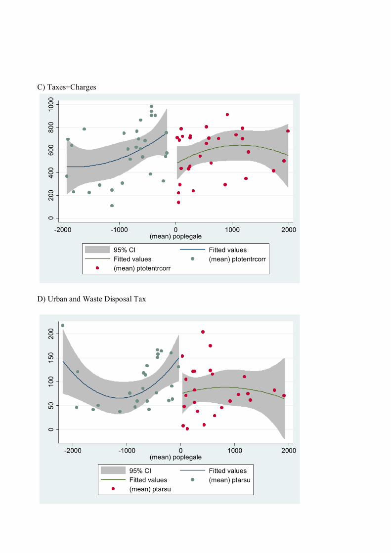
to overlap. Interestingly, we repeat the same graphical analysis (Fig 2) , by …tting the previous

…nancial variables with a quadratic polynomial of the legal population of the municipalities

switching from one regime to the other and the graphs are very similar to those obtained with

the actual population, con…rming the close correlation between legal population and actual

population and so the necessity to use a regression discountinuity design.

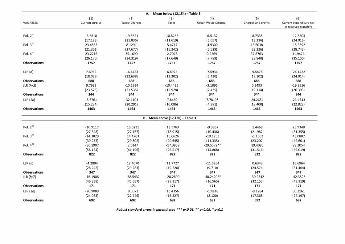
Finally we made a robustness check of our results by running a placebo test (Table 3) for

both the polynomial and the local linear regressions. We use the sample between 10,000 and

20,000 and de…ne in the sub-sample of the small municipalities a threshold corresponding to the

median population (12,154) and we do the same for the large sample municipalities …nding a

median population of 17,130. We run the same regressions that we have done with the 15,000

threshold, but the coe¢cient accounting for the threshold e¤ect is never signi…cant, either with

the speci…cations with covariates, or without covariates.

6 Conclusions

We tested on italian municipalities the impact on …scal policies of adopting two di¤erent elec-

toral systems: one for municipalities with less than 15,000 inhabitans where the mayor is elected

according to a plurality single-ballot regime with a unique list supporting her/him and the other

for municipalities with more than 15,000 inhabitans where the mayor is elected according to

a plurality double-ballot regime with a coalition of list supporting her/him. We use a panel

dataset 2001-2006 of all Italian municipalities including …nancial socio-economic and political

data. We exploit, either the between, and the within dimension of the dataset by applying the

di¤erence-in-di¤erence method to a regression discontinuity analysis.

Our test looks at the e¤ect of the two electoral systems on expenditure and revenue side.

We …nd that in the large-municipality electoral regime implies lower percapita taxes to …nanace

the same per-capita expenditure. Our results hold with both a polynomial aproximation and a

local linear regression method.

14

7 References

Alesina, A. and Drazen, A. (1991), "Why are stabilizations delayed? A political economy

model", American Economic Review, 81, 1170-1188.

Austen-Smith, D. (2000), "Redistributing income under proportional representation", Jour-

nal of Political Economy, 108, 1235-69.

Barbera A., (1993), Introduzione: una legge di transizione in un periodo di transizione, in

Barbera A. , Elezione diretta del sindaco, del presidente della provincia, del consiglio comunale

e del consiglio provinciale. Commento alla legge 25 marzo 1993, n.81, Rimini, Maggioli.

Besley, T., and A.C. Case (1995), "Does Political Accountability A¤ect Economic Policy

Choices? Evidence from Gubernatorial Term Limits", Quarterly Journal of Economics, 110,

769-98.

Bordignon, M., Nannicini, T., G. Tabellini (2010), "Moderating Political Extremism: Single

Round vs Runo¤ elections under Plurality Rule", mimeo, Bocconi University, Milan.

Bouton, L. (2010), "A Theory of Strategic Voting in Election Run-o¤", mimeo, Boston

University,

Cox, G. (1997), Making votes count, Cambridge University Press, Cambridge UK.

Dixit, A. and J. Londregan (1998), "Ideology, Tactics, and E¢ciency in Redistributive

Politics", Quarterly Journal of Economics, 113, 497-529.

Egger, P., and M. Koethenbuerger (2009), "Government Spending and Legislative Orga-

nization: Quasi-Experimental Evidence from Germany", forthcoming in American Economic

Journal: Applied Economics.

Fujiwara, T., (2010), “A Regression Discontinuity Test of Strategic Voting and Duverger’s

Law,” mimeo, Department of Economics, UBC.

Fabbrini, S. (2001), "Features and Implications of Semi-Parlamentarism: the Direct Election

of Italian Mayors", South European Society & Politics, 6, 47-70.

Gagliarducci, S. and T. Nannicini (2011) “Do better paid politicians perform better? Dis-

entangling incentives from selection”, Journal of the European Economic Association, forth-

coming.

Hallerberg, M. and von Hagen, J. (1999), "Electoral institutions, cabinet negotiations, and

budget de…cits in the European Union" In Poterba, J. and Von Hagen, J. (Eds.), Fiscal insti-

tutions and …scal performance, 209-232. Chicago IL: University of Chicago Press.

Lijphart, A. (1984). Democracies: Patterns of majoritarian and consensus government in

twenty-one countries, New Haven: Yale University Press.

List, J. A. and D. Sturm (2006), "How Elections Matter: Theory and Evidence from Envi-

15

ronmental Policy", Quarterly Journal of Economics, 121, 1249-1281.

Lizzeri, A. and N. Persico (2001), "The Provision of Public Goods under Alternative Elec-

toral Incentives", American Economic Review, 91, 225-45.

Martinelli, C. (2002), "Simple Plurality versus Plurality Runo¤ with Privately Informed

Voters" Social Choice and Welfare, 19.4, 901-919.

Mayerson, R. (1993), “E¤ectiveness of Electoral Systems in Reducing Government Corrup-

tion: a Game-theoretic Analysis", Games and Economic Behavior, 5, 118-32.

Milesi-Ferretti, G.-M., R. Perotti and M. Rostagno (2002), "Electoral Systems and the

Composition of Public Spending", Quarterly Journal of Economics, 117, 609-57.

Perotti, R. and Kontopoulos, Y. (2002), Fragmented …scal policy, Journal of Public Eco-

nomics, 86, 191-222.

Persson, T and G. Tabellini (2000), Political Economics: Explaining Economic Policy, MIT

Press (MA).

Persson, T. and G. Tabellini (2003), The Economic E¤ects of Constitutions: What do the

Data Say?, MIT Press (MA).

Petterson-Lidbom, P. (2008), "Does the Size of the Legislature A¤ect the Size of Govern-

ment? Evidence from Two Natural Experiments", mimeo, Stockholm University.

Ricciuti, R. (2004), "Political Fragmentation and Fiscal Outcomes", Public Choice, 118,

365-388.

Roubini, N. and Sachs, J. (1989), "Political and economic determinants of budget de…cits

in the industrial economies", European Economic Review, 33, 903-938.

Scarciglia R. (1993), Elezione diretta del sindaco e del presidente della provincia. Nomina

della giunta, in Barbera A. , Elezione diretta del sindaco, del presidente della provincia, del

consiglio comunale e del consiglio provinciale. Commento alla legge 25 marzo 1993, n.81,

Rimini, Maggioli.

8 Data Appendix

List of variablesFinancial variables: from the Italian Ministry of Interior

(http://…nanzalocale.interno.it/sitophp/home_…nloc.php?Titolo=Certi…cati+Consuntivi)

² Taxes: real total direct taxes by municipality (year 2006 constant euros per capita).

² Charges : real charges and pro…ts by municipality (year 2006 constant euros per capita).

16

² Urban waste disposal tax : real tax for waste disposal by municipality (year 2006 constant

euros per capita).

² Current Expenditure: real total current public expenditure (year 2006 constant euros per

capita).

² Political variables: authors’ elaboration on data from from the Italian Ministry of

Interior (http://amministratori.interno.it/AmmIndex5.htm and from

http://elezionistorico.interno.it/index.php?tp=G)

² Large: dummy variable equal to one when the mayor of the municipality is elected accord-

ing to to a double-ballot/multiple list electoral system, and whene the electoral system is

single ballot/ single list.

² Termlimit : dummy variable equal to one when the mayor of the municipality cannot

run for the next election because he/she is spending his/her second mandate, and zero

otherwise.

² Voteshare: percentage of votes obtained by the mayor when elected (the variable refers

to the …rst round for the double-ballot municipalities)

Demographic and socio-economic variables: from the Italian Ministry of Interior

(http://…nanzalocale.interno.it/ser/ispett.html) and from the Italian Institute of Statis-

tics (ISTAT - www.istat.it/dati/catalogo/20061102_00/)

² Income: real personal income tax base (year 2006 constant euros per capita).

² Population: state population divided by 1000.

² Aged: share of population over 65 years old.

² Child : share of population between 0 and 14 years old.

17

Table 1: Fixed effects estimates with year (2001-2006) and covariates controls. Independent variables: Dual Ballot dummy. (1) (2) (3) (4) (5) (6) VARIABLES Current

surplus Taxes + Charges

Taxes Urban Waste Disposal

Charges and profits

Current expenditure net of received transfers

Pol. 4 -33.5262** -81.5924*** -46.7595*** -23.5528*** -34.8340*** -48.0763*** (15.057) (15.939) (12.530) (7.349) (9.656) (16.399) R-squared 0.4558 0.9064 0.9086 0.6819 0.8420 0.8547 Pol. 3 -32.5389** -85.6505*** -46.7829*** -24.3663*** -38.8689*** -53.1215*** (15.005) (15.905) (12.358) (7.322) (9.698) (16.419) R-squared 0.4558 0.9064 0.9086 0.6819 0.8419 0.8547 Pol. 2 -30.3756** -91.1187*** -49.0185*** -27.7247*** -42.1017*** -60.7528*** (14.942) (15.888) (12.197) (7.344) (9.731) (16.512) R-squared 0.4557 0.9063 0.9086 0.6814 0.8419 0.8546 Observations 38,511 38,512 38,517 38,517 38,512 38,514

Robust standard errors in parentheses *** p<0.01, ** p<0.05, * p<0.1

Robust standard errors in parentheses *** p<0.01, ** p<0.05, * p<0.1

A. Estimations with covariates - Table 2 (1) (2) (3) (4) (5) (6) VARIABLES Current surplus Taxes+Charges Taxes Urban Waste Disposal Charges and profits Current expenditure net

of received transfers Pol. 2nd -50.7117** -61.7174*** -48.8992*** -26.6335*** -12.8182 -11.0057 (25.423) (22.228) (17.330) (8.967) (15.403) (25.884) Pol. 3nd -52.0351**

(24.761)

-64.7956*** (22.837)

-48.7996*** (17.250)

-26.2985*** (8.749)

-15.9959 (15.510)

-12.7605 (24.926)

Pol. 4nd -53.7419* (30.160)

-70.9977*** (24.437)

-47.0816** (18.835)

-30.3703*** (9.609)

-23.9160 (17.465)

-17.2558 (30.831)

Observations 2,579 2,579 2,579 2,579 2,579 2,579 LLR (h) -62.1552**

(27.345)

-74.8752** (29.704)

-37.4715 (24.037)

-33.8685*** (12.731)

-37.4037* (21.333)

-12.7200 (29.234)

Observations 493 493 493 493 493 493 LLR (h/2) -96.7916**

(46.943)

-17.7441 (41.407)

-23.6429 (35.525)

-18.1836 (14.363)

5.8988 (20.743)

79.0475 (49.206)

Observations 243 243 243 243 243 243

LLR (2h) -63.5675** (27.345)

-71.7752*** (25.305)

-45.4489** (19.871)

-33.4006*** (10.373)

-26.3263 (17.868)

-8.2077 (28.234)

Observations 981 981 981 981 981 981

B. Estimations without covariates - Table 2 Pol. 2nd -42.3671

(25.880)

-54.6013*** (20.751)

-41.0893** (16.391)

-19.3778** (9.097)

-13.5120 (13.539)

-12.2341 (26.001)

Pol. 3nd -44.4530* (25.072)

-64.4940*** (22.788)

-49.1054*** (17.285)

-26.4841*** (8.786)

-15.3886 (15.413)

-11.9116 (24.787)

Pol. 2nd -47.7953 (30.723)

-61.4079*** (22.897)

-40.7751** (17.978)

-22.2625** (9.883)

-20.6327 (15.620)

-24.2480 (27.368)

Observations 2,579 2,579 2,579 2,579 2,579 2,579 LLR (h) -64.9612**

(29.590)

-66.4215*** (24.842)

-35.0414* (19.495)

-16.2632 (11.051)

-31.3800** (15.933)

-1.4603 (27.767)

Observations 493 493 493 493 493 493 LLR (h/2) -128.7826***

(37.564)

-64.9081** (31.064)

-44.5207 (27.907)

-17.3277 (10.853)

-20.3874* (11.691)

63.8745* (35.543)

Observations 243 243 243 243 243 243

LLR (2h) -52.0010** (26.252)

-59.2497*** (22.408)

-34.8345** (17.438)

-19.8496** (9.957)

-24.4151 (14.987)

-7.2487 (26.604)

Observations 981 981 981 981 981 981

Robust standard errors in parentheses *** p<0.01, ** p<0.05, * p<0.1

A. Mean below (12,154) – Table 3 (1) (2) (3) (4) (5) (6) VARIABLES Current surplus Taxes+Charges Taxes Urban Waste Disposal Charges and profits Current expenditure net

of received transfers Pol. 2nd -6.6818

(17.128)

-19.5621 (21.836)

-10.8286 (11.619)

-6.5137 (5.057)

-8.7335 (19.236)

-12.8803 (24.016)

Pol. 3nd 23.4883 (21.361)

8.1291 (27.677)

-5.4747 (15.242)

-4.9300 (6.529)

13.6038 (23.226)

-15.3592 (28.743)

Pol. 4nd 23.2216 (26.170)

35.1690 (34.319)

-2.7073 (17.649)

0.2269 (7.789)

37.8763 (28.840)

11.9474 (35.150)

Observations 1757 1757 1757 1757 1757 1757 LLR (h) 7.6969

(18.029)

-16.4453 (22.638)

-6.8975 (12.302)

-7.5934 (5.430)

-9.5478 (19.102)

-24.1422 (24.014)

Observations 688 688 688 688 688 688 LLR (h/2) 9.7982

(23.575)

-10.1934 (21.535)

-10.4426 (15.928)

-3.1895 (7.435)

0.2493 (19.114)

-19.9916 (26.393)

Observations 344 344 344 344 344 344

LLR (2h) -8.6761 (15.224)

-32.1103 (20.201)

-7.8450 (10.086)

-7.7819* (4.381)

-24.2654 (18.400)

-23.4343 (22.822)

Observations 1463

1463 1463 1463 1463 1463

B. Mean above (17,130) – Table 3 Pol. 2nd -10.9117

(27.548)

15.0231 (27.167)

13.5763 (18.915)

-9.3867 (10.436)

1.4468 (21.987)

25.9348 (31.355)

Pol. 3nd -14.3829 (39.233)

14.4763 (29.802)

15.6626 (20.645)

-10.1753 (11.335)

-1.1862 (23.207)

43.0807 (42.601)

Pol. 4nd -86.1907 (58.164)

2.0147 (41.196)

-17.3939 (26.517)

-29.5572** (14.868)

19.4085 (31.516)

88.2054 (59.019)

Observations 822 822 822 822 822 822 LLR (h) -4.2894

(28.242)

12.4070 (29.283)

11.7727 (19.220)

-11.5264 (9.710)

0.6343 (24.574)

16.6964 (31.464)

Observations 347 347 347 347 347 347 LLR (h/2) -16.1906

(46.838)

-58.5432 (45.687)

-28.2890 (29.317)

-40.2420** (16.565)

-30.2542 (32.153)

-42.3526 (43.319)

Observations 171 171 171 171 171 171 LLR (2h) Observations 692

-20.9089 (24.063)

9.3072 (22.746)

692 692

18.4356 (16.327)

692

-1.4148 (8.120)

692

-9.1284 (17.368)

30.2161 (27.197)

692

Figure 1 A) Surplus

3040

5060

7080

-5000 0 5000(mean) pop_tot

95% CI Fitted valuesFitted values

B) Taxes

300

350

400

450

-5000 0 5000(mean) pop_tot

95% CI Fitted valuesFitted values

C)Taxes+Charges

400

450

500

550

600

650

-5000 0 5000(mean) pop_tot

95% CI Fitted valuesFitted values

D) Urban and Waste Disposal Tax

4050

6070

8090

-5000 0 5000(mean) pop_tot

95% CI Fitted valuesFitted values

Figure 2 A) Surplus

-100

010

020

030

0

-2000 -1000 0 1000 2000(mean) poplegale

95% CI Fitted valuesFitted values (mean) saldocorr2(mean) saldocorr2

B) Taxes

020

040

060

080

0

-2000 -1000 0 1000 2000(mean) poplegale

95% CI Fitted valuesFitted values (mean) ptottrib(mean) ptottrib

C) Taxes+Charges

020

040

060

080

010

00

-2000 -1000 0 1000 2000(mean) poplegale

95% CI Fitted valuesFitted values (mean) ptotentrcorr(mean) ptotentrcorr

D) Urban and Waste Disposal Tax

050

100

150

200

-2000 -1000 0 1000 2000(mean) poplegale

95% CI Fitted valuesFitted values (mean) ptarsu(mean) ptarsu