CO2 EMISSIONS, RENEWABLE ENERGY CONSUMPTION, … · This study aims investigating the relationship...

Bilgi Ekonomisi ve Yönetimi Dergisi / 2013 Cilt: VIII Sayı: II

Tüm hakları BEYDER’e aittir 89 All rights reserved by The JKEM

CO2 EMISSIONS, RENEWABLE ENERGY CONSUMPTION, POPULATION DENSITY

AND ECONOMIC GROWTH IN G7 COUNTRIES

Fatma Fehime AYDIN1

Abstract

This study aims investigating the relationship between CO2 emissions, renewable energy consumption,

economic growth, and population density in G7 countries for 1991–2009 period. In this study, Levin, Lin and

Chu; Breitung; Im, Pesaran and Shin; ADF- Fisher Chi-square; ADF- Choi Z-stat; PP- Fisher Chi-square and

PP- Choi Z-stat panel unit root tests, Johansen-Fisher panel cointegration test, panel Granger causality test,

impulse-response test and Panel OLS, fixed effects, random effects tests were employed. As a result of the study

we can say that from country to country the relationship between our variables may show difference, but

ultimately we have presented evidence that economic growth, renewable energy consumption and population

density are the causes of CO2 emissions.

Keywords: Carbondioxide emissions, renewable energy consumption, population density, economic growth,

G7.

Introduction

As one of the main problems of economics, economic growth is one of the main objectives of

most of the countries for many years. Income growth is vital for achieving economic, social,

and even political development. Countries that grow strongly for sustained periods of time are

able to reduce their poverty levels significantly, strengthen their democratic and political

stability, improve the quality of their natural environment, and even diminish the incidence of

crime and violence (Loayza and Soto 2002).

Until the 1970s economic growth and development focused on only increasing per capita

incomes and improving the welfare levels, i.e. only on read-economic growth. After this year,

starting to expressing the opinion that social development should not limited with only

economy, should also cover environment, nature and the needs of future generations, has led

to an increase in the criticisms of the traditional development model (Acar 2002). Carbon

dioxide (CO2) emissions come in at the beginning of the factors that negatively effect the

environment and the nature. CO2 emissions accumulate in the atmosphere and create costly

changes in regional climates throughout the world. Due to these losses of CO2 emissions,

researchers have interested more in the factors increasing and decreasing CO2 emissions.

In this regard, this study aims investigating the relationship between CO2 emissions and

renewable energy consumption, population density and economic growth in G7 countries for

1991–2009 periods. The reason for choosing G7 countries as sample is that, G7 economies

have caused 27.7% of World's total CO2 emissions in 2009 (WDI, World Development

Indicators 2013).

The paper is organized as follows: Next section is devoted to the literature. Section 3 presents

the data, methodology and results. Finally, Section 4 concludes.

1 Bingol University Faculty of Economics and Administrative Sciences Bingol/TURKEY [email protected]

mailto:[email protected]

The Journal of Knowledge Economy & Knowledge Management / Volume: VIII FALL


1. Literature Review

The relationship between CO2 emissions, economic growth, renewable energy consumption

and population density has been treated in the literature using different methodological

approaches. The results have differed significantly depending on the country, period,

variables and method used for the analysis.

The studies examining the relationship between economic growth and CO2 emissions have

reached three different conclusions. Kim et al. (2010, for linear causality), Ozturk and

Acaravci (2010), Jayanthakumaran et al. (2012, for India), Saboori et al. (2012, for short run)

concluded that there is no causal relationship between economic growth and CO2 emissions.

Lotfalipour et al. (2010), Jayanthakumaran et al. (2012, for China), Saboori et al. (2012, for

long run) concluded that there is a unidirectional causality from economic growth to CO2

emissions. Kim et al. (2010, for nonlinear causality), Shahbaz et al. (2013), Park and Hong

(2013) and Wang (2013) concluded that there is bidirectional causality between economic

growth and CO2 emissions.

Table 1 Summary of recent literature review for economic growth and CO2 emissions

Study Period Country Methodology Confirmed hypothesis

Kim, Lee and Nam

(2010)

1992-

2006

Korea Smooth transition autoregressive model,

linear and nonlinear Granger causality

tests

Linear causality: no

causality;

nonlinear causality: two-

way causality

Ozturk and Acaravci

(2010)

1968-

2005

Turkey ARDL cointegration analysis, Engle

Granger causality

Long run relationship;

No causality

Lotfalipour, Falahi

and Ashena (2010)

1967-

2007

Iran Unit root, Toda-Yamamoto causality Unidirectional causality

from economic growth to

CO2 emissions

Jayanthakumaran,

Verma and Liu

(2012)

1971-

2007

China and

India

Bounds testing approach to cointegration

and the ARDL methodology

In China: growth→CO2

emissions

In India: no causal

relationship

Saboori, Sulaiman

and Mohd (2012)

1980-

2009

Malaysia ARDL methodology, VECM Granger

Causality

U shape relationship

Short run: no causality

Long run: Unidirectional

causality from economic

growth to CO2 emissions

Arouri, Youssef,

M’Henni and Rault

(2012)

1981-

2005

12 MENA

countries

Panel unit root and cointegration tests Quadratic relationship

Shahbaz, Hye, Tiwari

and Leitao (2013)

1975-

2011

Indonesia Unit root, ARDL bounds, VECM

Granger causality, innovative accounting

approach

Bidirectional causality

Park and Hong

(2013)

1991-

2011

South Korea Regression analysis, Markov switching

model

Very close correlation,

variables are moving

identically

Wang (2013) 1971-

2007

138 countries Panel data analysis, quantile regression

analysis, short run error correction model

Absolute decoupling

Relative decoupling

Feedback

The studies examining the relationship between renewable energy consumption and CO2

emissions have reached three different conclusions. Menyah and Wolde-Rufael (2010) have

used Granger causality test and generalized impulse response approach for the period 1960-



2007 in US. They concluded that there is no causal relationship between renewable energy

consumption and CO2 emissions. Sadorsky (2009), Marques et al. (2010), Shafiei and Salim

(2012) and Farhani (2013, for long run) concluded that there is a unidirectional causality from

CO2 emissions to renewable energy consumption. Tiwari (2011), Shabbir et al. (2011), Silva

et al. (2012), Kulionis (2013) and Farhani (2013, for short run) concluded that there is a

unidirectional causality from renewable energy consumption to CO2 emissions.

Table 2 Summary of recent literature review for renewable energy consumption and CO2 emissions


Sadorsky (2009) 1980-

2005

G7 Vector auto regression techniques Unidirectional causality from CO2

emissions to renewable energy

consumption

Menyah and

Wolde-Rufael

(2010)

1960-

2007

US Granger Causality test, generalized

impulse-response approach

No causality

Marques et al.

(2010)

1990-

2006

24 EU countries Panel regression techniques Unidirectional causality from CO2


consumption

Tiwari (2011) 1960-

2009

India Structural Vector Auto Regression

Analysis

Unidirectional causality from

renewable energy consumption to

CO2 emissions

Shabbir et al.

(2011)

1971-

2010

Pakistan Clemente-Montanes-Reyes

detrended structural break unit root

test, ARDL bounds test



CO2 emissions

Silva et al.

(2012)

1960-

2004

USA, Denmark,

Portugal and

Spain

Unit root, impulse-response

function



CO2 emissions

Shafiei and

Salim (2012)

1980-

2008

29 OECD

countries

STIRPAT model, panel unit root,

panel cointegration, panel DOLS

and panel causality tests

Unidirectional causality from CO2


consumption

Kulionis (2013) 1972-

2012

Denmark Unit root, Toda-Yomamoto Granger

causality, cointegration, impulse

response function



CO2 emissions

Farhani (2013) 1975-

2008

12 MENA

countries

Panel unit root, panel cointegration,

panel causality, panel FMOLS and

DOLS tests

Short run: unidirectional causality

from renewable energy

consumption to CO2 emissions

Long run: unidirectional causality

from CO2 emissions to renewable

energy consumption

The studies examining the relationship between population and CO2 emissions have reached

four different conclusions. Knapp and Mookerjee (1996) used cointegration analysis, granger

causality and ECM causality for the period 1880-1989. They concluded that there is a

unidirectional causality from CO2 emissions to population. Dietz and Rosa (1997) and Shi

(2001) concluded that there is a unidirectional causality from population to CO2 emissions.

Lantz and Feng (2006) used five region panel data analysis for the period 1970-2000 in

Canada. They concluded that there is an inverted U-shaped relationship between population

and CO2 emissions.

Martinez- Zarzoso et al. (2007) used STIRPAT model, panel OLS, fixed effects and random

effects model and Generalized method of moments (GMM) test for the period 1975-1999 in

23 EU countries. Their results show that the impact of population growth on emissions is

more than proportional for recent accession countries whereas for old EU members, the



elasticity is lower than unity and non significant when the properties of the time series and the

dynamics are correctly specified.

Jorgenson and Clark (2010) used cross national panel study for the period 1960-2005 in 86

countries. They concluded that there is a large and stable positive association between

population and CO2 emissions.

Table 3 Summary of recent literature review for Population and CO2 emissions


Knapp and

Mookerjee (1996)

1880-

1989

World Cointegration analysis, Granger causality,

ECM causality

Unidirectional causality

from CO2 emissions to

population

Dietz and Rosa

(1997)

1989 111 countries Impact=Population·Affluence·Technology

(IPAT) model

Unidirectional causality

from population to CO2

emissions

Shi (2001) 1975-

1996

93 countries Descriptive analysis, fixed effects model Unidirectional causality

from population to CO2

emissions

Lantz and Feng

(2006)

1970-

2000

Canada Five-region panel data analysis Inverted U-shaped

relationship

Martínez-Zarzoso

et al. (2007)

1975-

1999

23 EU

countries

STIRPAT model, OLS, fixed effects and

random effects model, Generalized

method of moments (GMM)

The elasticity of

emissions-population is

much lower for old EU

members then recent

accession countries

Jorgenson and

Clark (2010)

1960-

2005

86 countries Cross-national panel study a large and stable positive

association

This paper analyzes the relationship between CO2 emissions, economic growth, renewable

energy consumption and population density.

2. Data, Methodology and Results

2.1. Data

In our study carbon dioxide emissions are in metric tons per capita, representing economic

growth GDP is in current US dollars, renewable energy consumption is share of renewable in

primary consumption (%), and population density is people per square kilometer of land area.

Data set covers 1991–2009 period in G7 countries and attained from Enerdata energy

statistical yearbook 2013 and World Bank.

In our study the main model we examine is:

itCO2ln itititit epopdensrerugdp lnln 321

2.2. Panel Unit Root Test

In panel data models, the leading studies proposed unit root test are Levin, Lin and Chu

(2002), Breitung (2000), Im, Pesaran and Shin (2003), Maddala and Wu (1999) and Choi

(2001). In our study these unit root tests are applied.

Levin, Lin and Chu (LLC) and Breitung tests assume that there is a common unit root

process. And these tests employ a null hypothesis of a unit root. LLC and Breitung tests

consider the following basic ADF specification:

http://www.sciencedirect.com/science/article/pii/S0921800911000814#bb0165

http://www.sciencedirect.com/science/article/pii/S0921800911000814#bb0165



ip

j

ititjitijitit Xyyy1

1 .

Here y indicates the series to be done unit root test, Δ indicates the first order difference

processor, i indicates cross section units or series, t indicates periods, itX indicates the

exogenous values in the model and indicates errors.

The null and alternative hypotheses for the tests may be written as:

0:

0:

1

0

H

H

Under the null hypothesis there is a unit root, under the alternative hypothesis there is no unit

root (Levin et al., 2002; and Breitung, 2000).

The Im, Pesaran and Shin (IPS) and the Fisher ADF and PP tests assume that there is an

individual unit root process. These tests are characterized by the combining of individual unit

root tests to derive a panel-specific result.

The null and alternative hypotheses for the IPS test may be written as:

NNNifor

NiforH

iallforH

i

i

i

,,2,1,0

,,2,1,0:

,0:

1

1

0

which may be interpreted as a non-zero fraction of the individual processes is stationary (Im

et al., 2003).

Maddala and Wu (1999) used the Fisher (1932) test results which are based on combining the

p-values of the test statistic for a unit root in each cross section. If we define i as the p-value

from any individual unit root test for cross section i, that i are U[0,1] and independent, and

ie log2 has a 2 distribution with 2 degrees of freedom. The null and alternative

hypotheses are the same as in the IPS test. Applying the ADF estimation equation in each

cross-section, we can compute the ADF t-statistic for each individual series, find the

corresponding p-value from the empirical distribution of ADF t-statistic, and compute the

Fisher-test statistics and compare it with the appropriate 2 critical value (Hoang and

McNown, 2006).



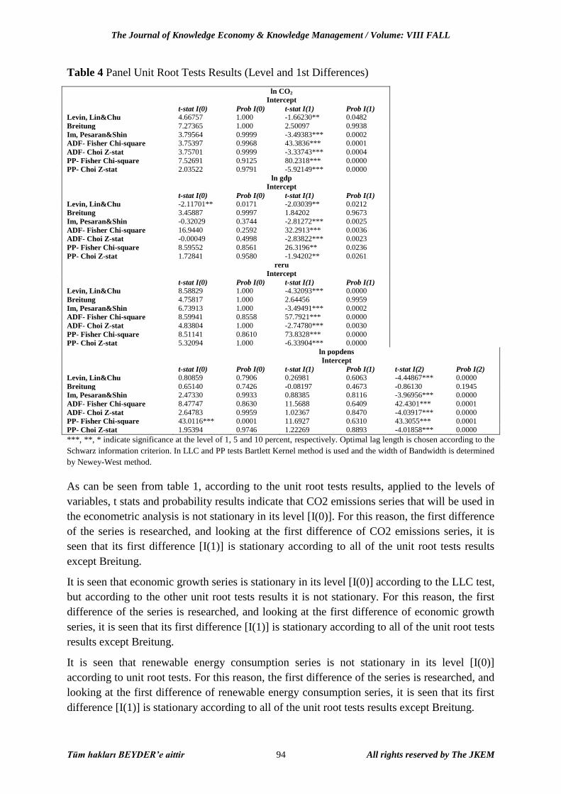
Table 4 Panel Unit Root Tests Results (Level and 1st Differences)

ln CO2

Intercept

t-stat I(0) Prob I(0) t-stat I(1) Prob I(1)

Levin, Lin&Chu 4.66757 1.000 -1.66230** 0.0482

Breitung 7.27365 1.000 2.50097 0.9938

Im, Pesaran&Shin 3.79564 0.9999 -3.49383*** 0.0002

ADF- Fisher Chi-square 3.75397 0.9968 43.3836*** 0.0001

ADF- Choi Z-stat 3.75701 0.9999 -3.33743*** 0.0004

PP- Fisher Chi-square 7.52691 0.9125 80.2318*** 0.0000

PP- Choi Z-stat 2.03522 0.9791 -5.92149*** 0.0000

ln gdp

Intercept


Levin, Lin&Chu -2.11701** 0.0171 -2.03039** 0.0212

Breitung 3.45887 0.9997 1.84202 0.9673

Im, Pesaran&Shin -0.32029 0.3744 -2.81272*** 0.0025


ADF- Choi Z-stat -0.00049 0.4998 -2.83822*** 0.0023

PP- Fisher Chi-square 8.59552 0.8561 26.3196** 0.0236

PP- Choi Z-stat 1.72841 0.9580 -1.94202** 0.0261

reru

Intercept


Levin, Lin&Chu 8.58829 1.000 -4.32093*** 0.0000

Breitung 4.75817 1.000 2.64456 0.9959

Im, Pesaran&Shin 6.73913 1.000 -3.49491*** 0.0002


ADF- Choi Z-stat 4.83804 1.000 -2.74780*** 0.0030

PP- Fisher Chi-square 8.51141 0.8610 73.8328*** 0.0000

PP- Choi Z-stat 5.32094 1.000 -6.33904*** 0.0000

ln popdens

Intercept t-stat I(0) Prob I(0) t-stat I(1) Prob I(1) t-stat I(2) Prob I(2)

Levin, Lin&Chu 0.80859 0.7906 0.26981 0.6063 -4.44867*** 0.0000

Breitung 0.65140 0.7426 -0.08197 0.4673 -0.86130 0.1945

Im, Pesaran&Shin 2.47330 0.9933 0.88385 0.8116 -3.96956*** 0.0000

ADF- Fisher Chi-square 8.47747 0.8630 11.5688 0.6409 42.4301*** 0.0001

ADF- Choi Z-stat 2.64783 0.9959 1.02367 0.8470 -4.03917*** 0.0000

PP- Fisher Chi-square 43.0116*** 0.0001 11.6927 0.6310 43.3055*** 0.0001

PP- Choi Z-stat 1.95394 0.9746 1.22269 0.8893 -4.01858*** 0.0000

***, **, * indicate significance at the level of 1, 5 and 10 percent, respectively. Optimal lag length is chosen according to the

Schwarz information criterion. In LLC and PP tests Bartlett Kernel method is used and the width of Bandwidth is determined

by Newey-West method.

As can be seen from table 1, according to the unit root tests results, applied to the levels of

variables, t stats and probability results indicate that CO2 emissions series that will be used in

the econometric analysis is not stationary in its level [I(0)]. For this reason, the first difference

of the series is researched, and looking at the first difference of CO2 emissions series, it is

seen that its first difference [I(1)] is stationary according to all of the unit root tests results

except Breitung.

It is seen that economic growth series is stationary in its level [I(0)] according to the LLC test,

but according to the other unit root tests results it is not stationary. For this reason, the first

difference of the series is researched, and looking at the first difference of economic growth

series, it is seen that its first difference [I(1)] is stationary according to all of the unit root tests

results except Breitung.

It is seen that renewable energy consumption series is not stationary in its level [I(0)]

according to unit root tests. For this reason, the first difference of the series is researched, and

looking at the first difference of renewable energy consumption series, it is seen that its first

difference [I(1)] is stationary according to all of the unit root tests results except Breitung.



And lastly, it is seen that population density series is stationary in its level [I(0)] according to

the PP-Fisher Chi-Square test, but according to the other unit root tests results it is not

stationary. For this reason, the first difference of the series is researched, and looking at the

first difference of population density series, it is seen that its first difference [I(1)] is not

stationary according to all of the unit root tests results. Then the second difference of the

series is researched, and looking at the second difference of population density series, it is

seen that its second difference [I(2)] is stationary according to all of the unit root tests results

except Breitung.

2.3. Panel Cointegration Test

In our study Johansen Fisher panel cointegration analysis was used after investigating unit

roots in order to investigate if in the long term there is a mutual relation between the series.

Johansen Fisher panel cointegration test is developed by Maddala and Wu (1999). As an

alternative test for cointegration in panel data, Maddala and Wu used Fisher's result to

propose a method for combining tests from individual cross-sections to obtain a test statistic

for the panel data. Two kinds of Johansen Fisher tests have been developed: the Fisher test

from the trace test and the Fisher test from the maximum eigen-value test (Sheigeyuki and

Yoichi, 2009).

We did not use population density variable in cointegration analysis because while other

variables are stationary in their first level, population density variable is not stationary in its

first level.

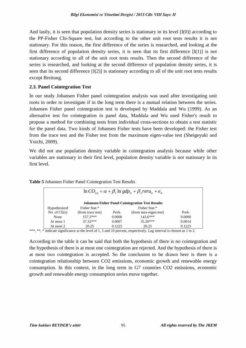
Table 5 Johansen Fisher Panel Cointegration Test Results

itCO2ln ititit ererugdp 21 ln

Johansen Fisher Panel Cointegration Test Results

Hypothesized

No. of CE(s)

Fisher Stat.*

(from trace test) Prob.

Fisher Stat.*

(from max-eigen test) Prob.

None 157.2*** 0.0000 143.6*** 0.0000

At most 1 37.32*** 0.0007 35.20*** 0.0014

At most 2 20.25 0.1223 20.25 0.1223

***, **, * indicate significance at the level of 1, 5 and 10 percent, respectively. Lag interval is chosen as 1 to 2.

According to the table it can be said that both the hypothesis of there is no cointegration and

the hypothesis of there is at most one cointegration are rejected. And the hypothesis of there is

at most two cointegration is accepted. So the conclusion to be drawn here is there is a

cointegration relationship between CO2 emissions, economic growth and renewable energy

consumption. In this context, in the long term in G7 countries CO2 emissions, economic

growth and renewable energy consumption series move together.



Table 6 Johansen Fisher Panel Cointegration Test Individual Cross Section Results

Individual cross section results

Trace Test Max-Eign Test

Cross Section Statistics Prob.** Statistics Prob.**

Hypothesis of no cointegration

1 38.7263 0.0036 26.7949 0.0072

2 45.6466 0.0004 32.7952 0.0008

3 73.9613 0.0000 46.3935 0.0000

4 78.1071 0.0000 63.4586 0.0000

5 57.2212 0.0000 41.0669 0.0000

6 33.8914 0.0160 28.0140 0.0046

7 71.0897 0.0000 62.8626 0.0000

Hypothesis of at most 1 cointegration relationship

1 11.9314 0.1603 10.9533 0.1566

2 12.8514 0.1204 11.5769 0.1276

3 27.5678 0.0005 22.6508 0.0019

4 14.6485 0.0668 13.8582 0.0579

5 16.1543 0.0397 15.5818 0.0308

6 5.8774 0.7100 4.5932 0.7920

7 8.2270 0.4414 7.5673 0.4244

Hypothesis of at most 2 cointegration relationship

1 0.9781 0.3227 0.9781 0.3227

2 1.2745 0.2589 1.2745 0.2589

3 4.9170 0.0266 4.9170 0.0266

4 0.7903 0.3740 0.7903 0.3740

5 0.5725 0.4493 0.5725 0.4493

6 1.2842 0.2571 1.2842 0.2571

7 0.6597 0.4167 0.6597 0.4167

**MacKinnon-Haug-Michelis (1999) p-values

When we look at the individual cross section results, according to both the trace test and max-

eigen test, in all the countries there is at most two cointegration relationships between

economic growth, CO2 emissions and renewable energy consumption.

2.4. Panel Granger Causality Test Findings and Evaluation

In our study Panel Granger causality test is used to examine if there is causality between CO2

emissions, economic growth, renewable energy consumption and popdens variables. Panel

Granger causality test is developed by Granger (1969) for the question of whether x causes

y . Granger’s method aims to see how much of the current y can be explained by past values

of y and then to see whether adding lagged values of x can improve the explanation. If x

helps in the prediction of y or if the coefficients on the lagged x ’s are statistically significant

then y is said to be Granger-caused by x . There can be also bi-directional causality, x

Granger causes y and y Granger causes x (Granger, 1969). There are many ways to

examine for Granger causality because of the assumptions of heterogeneity across countries

and time (Chen et al., 2013).

The simple two-variable causal model is as follows:

m

j

m

j

tjtjjtjt

m

j

m

j

tjtjjtjt

YdXcY

YbXaX

1 1

1 1



Here tX and tY are two stationary time series with zero means. t and t are two

uncorrelated white-noise series.

The null hypothesis is that x does not Granger-cause y in the first regression and that y

does not Granger-cause x in the second regression (Granger, 1969).

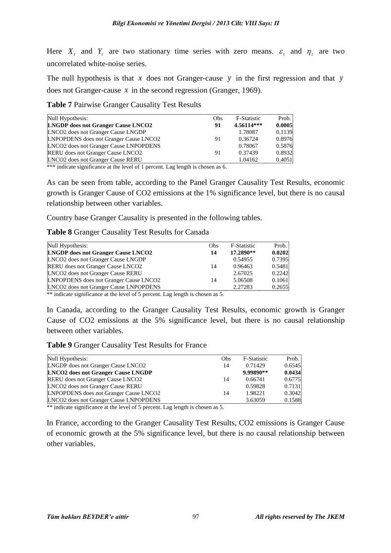
Table 7 Pairwise Granger Causality Test Results

Null Hypothesis: Obs F-Statistic Prob.

LNGDP does not Granger Cause LNCO2 91 4.56114*** 0.0005

LNCO2 does not Granger Cause LNGDP 1.78087 0.1139

LNPOPDENS does not Granger Cause LNCO2 91 0.36724 0.8976

LNCO2 does not Granger Cause LNPOPDENS 0.78067 0.5876

RERU does not Granger Cause LNCO2 91 0.37439 0.8932

LNCO2 does not Granger Cause RERU 1.04162 0.4051

*** indicate significance at the level of 1 percent. Lag length is chosen as 6.

As can be seen from table, according to the Panel Granger Causality Test Results, economic

growth is Granger Cause of CO2 emissions at the 1% significance level, but there is no causal

relationship between other variables.

Country base Granger Causality is presented in the following tables.

Table 8 Granger Causality Test Results for Canada


LNGDP does not Granger Cause LNCO2 14 17.2890** 0.0202






** indicate significance at the level of 5 percent. Lag length is chosen as 5.

In Canada, according to the Granger Causality Test Results, economic growth is Granger

Cause of CO2 emissions at the 5% significance level, but there is no causal relationship

between other variables.

Table 9 Granger Causality Test Results for France


LNGDP does not Granger Cause LNCO2 14 0.71429 0.6545

LNCO2 does not Granger Cause LNGDP 9.99890** 0.0434





** indicate significance at the level of 5 percent. Lag length is chosen as 5.

In France, according to the Granger Causality Test Results, CO2 emissions is Granger Cause

of economic growth at the 5% significance level, but there is no causal relationship between

other variables.



Table 10 Granger Causality Test Results for Germany







LNCO2 does not Granger Cause LNPOPDENS 149.636*** 0.0009

*** indicate significance at the level of 1 percent. Lag length is chosen as 5.

In Germany, according to the Granger Causality Test Results, CO2 emissions is Granger

Cause of population density at the 1% significance level, but there is no causal relationship

between other variables.

Table 11 Granger Causality Test Results for Italy


LNGDP does not Granger Cause LNCO2 14 14.8039** 0.0252




LNPOPDENS does not Granger Cause LNCO2 14 71.4824*** 0.0026


*** and ** indicate significance at the level of 1 and 5 percent, respectively. Lag length is chosen as 5.

In Italy, according to the Granger Causality Test Results, economic growth is Granger Cause

of CO2 emissions at the 5% significance level, and population density is granger cause of

CO2 emissions at the %1 significance level, but there is no causal relationship between CO2

emissions and renewable energy consumption variables.

Table 12 Granger Causality Test Results for Japan








Lag length is chosen as 5.

In Japan according to the Granger Causality Test Results, there is no causal relationship

between our variables.

Table 13 Granger Causality Test Results for United Kingdom Null Hypothesis: Obs F-Statistic Prob.







Lag length is chosen as 5.

In United Kingdom, according to the Granger Causality Test Results, there is no causal

relationship between our variables.



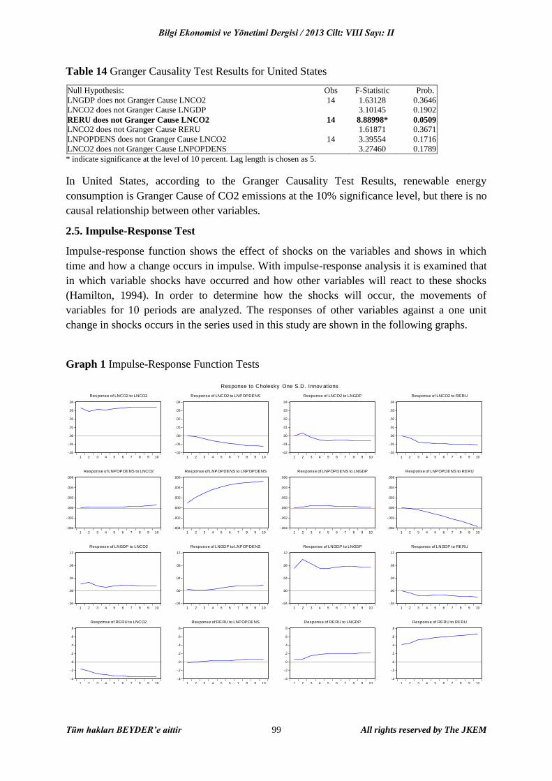
Table 14 Granger Causality Test Results for United States




RERU does not Granger Cause LNCO2 14 8.88998* 0.0509




* indicate significance at the level of 10 percent. Lag length is chosen as 5.

In United States, according to the Granger Causality Test Results, renewable energy

consumption is Granger Cause of CO2 emissions at the 10% significance level, but there is no

causal relationship between other variables.

2.5. Impulse-Response Test

Impulse-response function shows the effect of shocks on the variables and shows in which

time and how a change occurs in impulse. With impulse-response analysis it is examined that

in which variable shocks have occurred and how other variables will react to these shocks

(Hamilton, 1994). In order to determine how the shocks will occur, the movements of

variables for 10 periods are analyzed. The responses of other variables against a one unit

change in shocks occurs in the series used in this study are shown in the following graphs.

Graph 1 Impulse-Response Function Tests

-.02

-.01

.00

.01

.02

.03

.04

1 2 3 4 5 6 7 8 9 10

Response of LNCO2 to LNCO2

-.02

-.01

.00

.01

.02

.03

.04

1 2 3 4 5 6 7 8 9 10

Response of LNCO2 to LNPOPDENS

-.02

-.01

.00

.01

.02

.03

.04

1 2 3 4 5 6 7 8 9 10

Response of LNCO2 to LNGDP

-.02

-.01

.00

.01

.02

.03

.04

1 2 3 4 5 6 7 8 9 10

Response of LNCO2 to RERU

-.004

-.002

.000

.002

.004

.006

1 2 3 4 5 6 7 8 9 10

Response of LNPOPDENS to LNCO2

-.004

-.002

.000

.002

.004

.006

1 2 3 4 5 6 7 8 9 10

Response of LNPOPDENS to LNPOPDENS

-.004

-.002

.000

.002

.004

.006

1 2 3 4 5 6 7 8 9 10

Response of LNPOPDENS to LNGDP

-.004

-.002

.000

.002

.004

.006

1 2 3 4 5 6 7 8 9 10

Response of LNPOPDENS to RERU

-.04

.00

.04

.08

.12

1 2 3 4 5 6 7 8 9 10

Response of LNGDP to LNCO2

-.04

.00

.04

.08

.12

1 2 3 4 5 6 7 8 9 10

Response of LNGDP to LNPOPDENS

-.04

.00

.04

.08

.12

1 2 3 4 5 6 7 8 9 10

Response of LNGDP to LNGDP

-.04

.00

.04

.08

.12

1 2 3 4 5 6 7 8 9 10

Response of LNGDP to RERU

-.4

-.2

.0

.2

.4

.6

.8

1 2 3 4 5 6 7 8 9 10

Response of RERU to LNCO2

-.4

-.2

.0

.2

.4

.6

.8

1 2 3 4 5 6 7 8 9 10

Response of RERU to LNPOPDENS

-.4

-.2

.0

.2

.4

.6

.8

1 2 3 4 5 6 7 8 9 10

Response of RERU to LNGDP

-.4

-.2

.0

.2

.4

.6

.8

1 2 3 4 5 6 7 8 9 10

Response of RERU to RERU

Response to Cholesky One S.D. Innov ations



The impact of a shock of one standard deviation in economic growth on CO2 emissions

initially increases up to 0.0035, then becomes negative in third period, and beginning from the

fourth period continuously fluctuates between -0.005 and -0.006.

The impact of a shock of one standard deviation in population density and renewable energy

consumption on CO2 emissions monitors a negative course and gradually decreases.

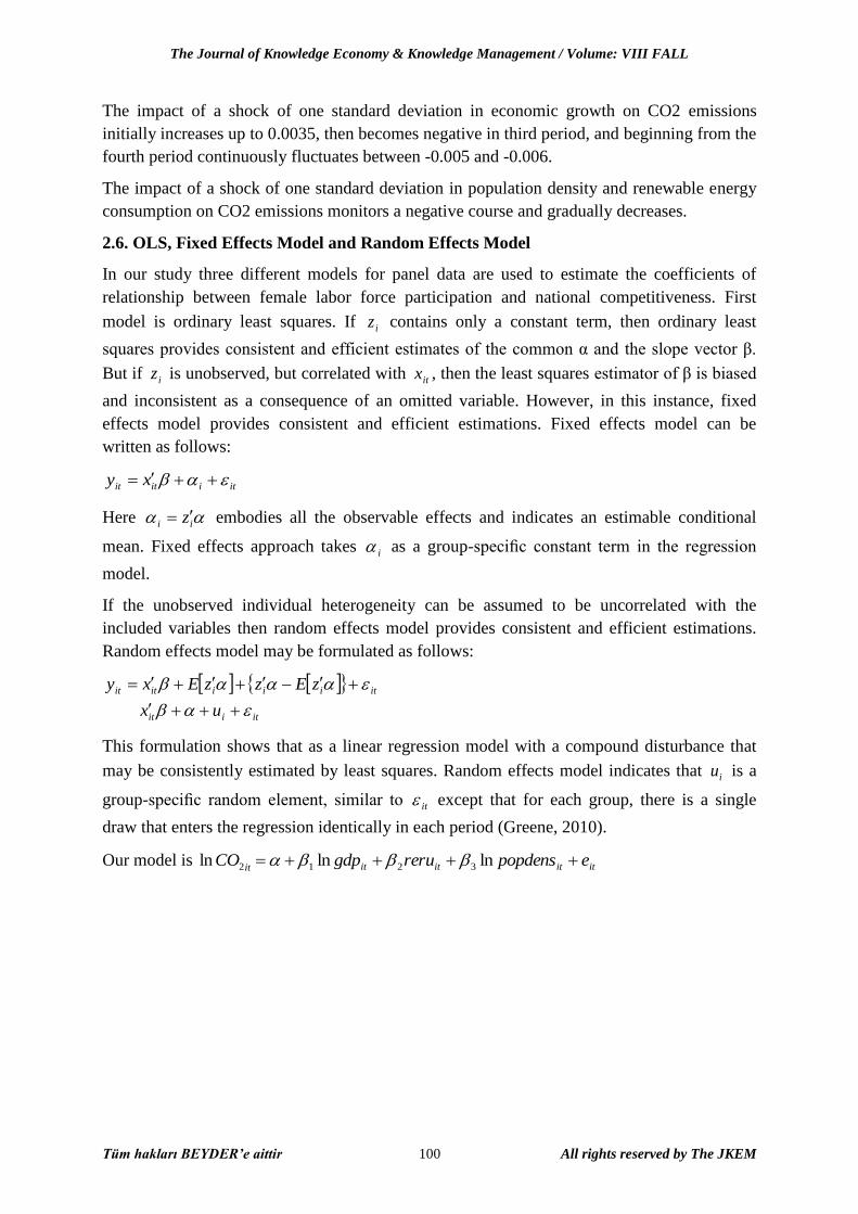
2.6. OLS, Fixed Effects Model and Random Effects Model

In our study three different models for panel data are used to estimate the coefficients of

relationship between female labor force participation and national competitiveness. First

model is ordinary least squares. If iz contains only a constant term, then ordinary least

squares provides consistent and efficient estimates of the common α and the slope vector β.

But if iz is unobserved, but correlated with itx , then the least squares estimator of β is biased

and inconsistent as a consequence of an omitted variable. However, in this instance, fixed

effects model provides consistent and efficient estimations. Fixed effects model can be

written as follows:

itiitit xy

Here ii z embodies all the observable effects and indicates an estimable conditional

mean. Fixed effects approach takes i as a group-specific constant term in the regression

model.

If the unobserved individual heterogeneity can be assumed to be uncorrelated with the

included variables then random effects model provides consistent and efficient estimations.

Random effects model may be formulated as follows:

itiit

itiiiitit

ux

zEzzExy

This formulation shows that as a linear regression model with a compound disturbance that

may be consistently estimated by least squares. Random effects model indicates that iu is a

group-specific random element, similar to it except that for each group, there is a single

draw that enters the regression identically in each period (Greene, 2010).

Our model is it

CO2ln itititit epopdensrerugdp lnln 321



Table 15 OLS, cross section fixed effects and cross section random effects tests results

OLS Cross Section

Fixed Effects

Cross Section

Random Effects

Constant -0.613279

(0,3751)

4.012734

(0.0000)

3.867214

(0.0000)

LNGDP 0.166028

(0.0000)

-0.013380

(0.6676)

-0.010939

(0.5305)

RERU -0.048305

(0.0000)

-0.020754

(0.0000)

-0.021435

(0.0000)

LNPOPDENS -0.326125

(0.0000)

-0.257234

(0.2439) -0.239373

(0.0001) R2 0.795526 0.988257 0.366977

F 167.2956

(0.0000)

1150.167

(0.0000)

24.92804

(0.0000)

According to table, all three models gave statistically significant results. To investigate which

one of these models is appropriate, we employed Hausman (1978) and Likelihood Ratio

Tests. Under the null hypothesis that the unobservable, individual-specific effects and the

regressors are orthogonal, Hausman specification test is based on the idea that the set of

coefficient estimates obtained from the fixed-effects estimation should not differ

systematically from the set obtained from random-effects estimation. If the test results suggest

rejecting the equality of both coefficient sets, then it can be said that fixed effects estimation

results is more appropriate than random effects estimation results. If this is the case than

random effects estimations are ignored (Frondel and Vance, 2010).

In panel data models, to test the validity of the classic model (OLS); i.e. there is whether the

unit and/or time effects, likelihood ratio test can be applied. Likelihood ratio test, that is used

to test classical model against the fixed effects model, is applied to determine in which model

framework the equation will be estimated. Likelihood ratio test research if standard errors of

unit effects are equal to zero; in other words, if the basic hypothesis that classical model is

appropriate ( 0:0 H ). If H0 is rejected than it can be said that classical model is not

appropriate (Gerni et al., 2012).

Likelihood ratio and Hausman tests have been applied to find the fittest of these models.

Likelihood ratio test has been applied to find the appropriate one of the OLS model and fixed

effects model. Hausman test has been applied to decide to use which one of the fixed effects

and random effects models. It is examined if the difference between the two model’s

parameters is statistically significant. Accordingly the results of the likelihood ratio test under

the null hypothesis of “the OLS estimator is correct” and the Hausman test under the null

hypothesis of “the random effects estimator is correct” are shown in the following table.

Table 16 Likelihood Ratio and Hausman Test Results

Test Summary

Statistic d.f. Prob.

Cross-Section F 336.460807 6.123 0.0000

Cross-Section Chi-Square 380.007747 6 0,0000

Cross-Section Random 4.101222 3 0.2507



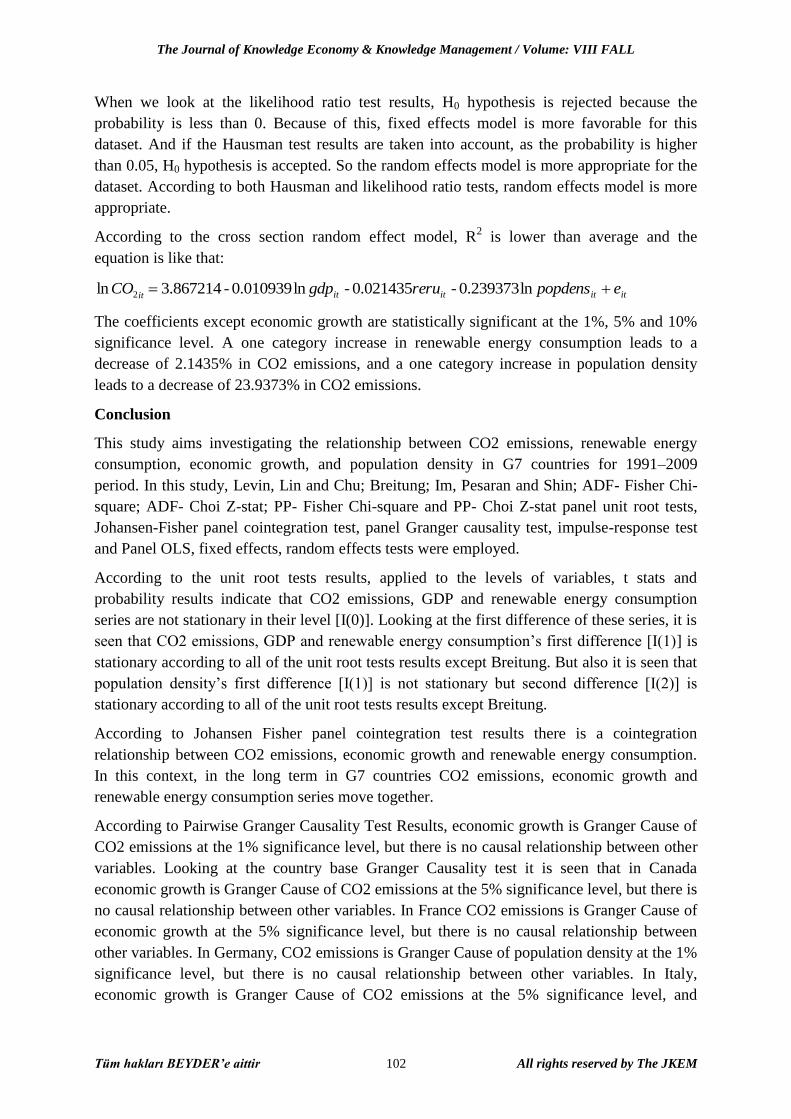
When we look at the likelihood ratio test results, H0 hypothesis is rejected because the

probability is less than 0. Because of this, fixed effects model is more favorable for this

dataset. And if the Hausman test results are taken into account, as the probability is higher

than 0.05, H0 hypothesis is accepted. So the random effects model is more appropriate for the

dataset. According to both Hausman and likelihood ratio tests, random effects model is more

appropriate.

According to the cross section random effect model, R2 is lower than average and the

equation is like that:

itCO2ln itititit epopdensrerugdp ln0.239373-0.021435-ln0.010939-3.867214

The coefficients except economic growth are statistically significant at the 1%, 5% and 10%

significance level. A one category increase in renewable energy consumption leads to a

decrease of 2.1435% in CO2 emissions, and a one category increase in population density

leads to a decrease of 23.9373% in CO2 emissions.

Conclusion

This study aims investigating the relationship between CO2 emissions, renewable energy

consumption, economic growth, and population density in G7 countries for 1991–2009

period. In this study, Levin, Lin and Chu; Breitung; Im, Pesaran and Shin; ADF- Fisher Chi-

square; ADF- Choi Z-stat; PP- Fisher Chi-square and PP- Choi Z-stat panel unit root tests,

Johansen-Fisher panel cointegration test, panel Granger causality test, impulse-response test

and Panel OLS, fixed effects, random effects tests were employed.

According to the unit root tests results, applied to the levels of variables, t stats and

probability results indicate that CO2 emissions, GDP and renewable energy consumption

series are not stationary in their level [I(0)]. Looking at the first difference of these series, it is

seen that CO2 emissions, GDP and renewable energy consumption’s first difference [I(1)] is

stationary according to all of the unit root tests results except Breitung. But also it is seen that

population density’s first difference [I(1)] is not stationary but second difference [I(2)] is

stationary according to all of the unit root tests results except Breitung.

According to Johansen Fisher panel cointegration test results there is a cointegration

relationship between CO2 emissions, economic growth and renewable energy consumption.

In this context, in the long term in G7 countries CO2 emissions, economic growth and

renewable energy consumption series move together.

According to Pairwise Granger Causality Test Results, economic growth is Granger Cause of

CO2 emissions at the 1% significance level, but there is no causal relationship between other

variables. Looking at the country base Granger Causality test it is seen that in Canada

economic growth is Granger Cause of CO2 emissions at the 5% significance level, but there is

no causal relationship between other variables. In France CO2 emissions is Granger Cause of

economic growth at the 5% significance level, but there is no causal relationship between

other variables. In Germany, CO2 emissions is Granger Cause of population density at the 1%

significance level, but there is no causal relationship between other variables. In Italy,

economic growth is Granger Cause of CO2 emissions at the 5% significance level, and



population density is granger cause of CO2 emissions at the %1 significance level, but there is

no causal relationship between CO2 emissions and renewable energy consumption variables.

In Japan and United Kingdom, there is no causal relationship between our variables. In United

States, according to the Granger Causality Test Results, renewable energy consumption is

Granger Cause of CO2 emissions at the 10% significance level, but there is no causal

relationship between other variables.

According to impulse-response test, the impact of a shock of one standard deviation in

economic growth on CO2 emissions initially increases up to 0.0035, then becomes negative in

third period, and beginning from the fourth period continuously fluctuates between -0.005 and

-0.006. The impact of a shock of one standard deviation in population density and renewable

energy consumption on CO2 emissions monitors a negative course and gradually decreases.

Lastly panel OLS, fixed effects and random effects tests were employed. And likelihood ratio

and Hausman tests have been applied to find the fittest of these models. According to both

Hausman and likelihood ratio tests, random effects model is more appropriate. According to

the results of cross section random effect model, a one category increase in renewable energy

consumption leads to a decrease of 2.1435% in CO2 emissions, and a one category increase in

population density leads to a decrease of 23.9373% in CO2 emissions.

To sum up, we can say that from country to country the relationship between our variables

may show difference, but ultimately we have presented evidence that economic growth,

renewable energy consumption and population density are the causes of CO2 emissions.

References

Acar Y. 2002. İktisadi Büyüme ve Büyüme Modelleri, Generalized 4th

press. Vipaş Publications, Publication

Number: 67, Bursa.

Arouri MEH, Youssef AB, M’henni H and Rault C. 2012. Energy Consumption, Economic Growth and CO2

Emissions in Middle East and North African Countries. Discussion Paper Series, IZA, DP No: 6412.

Breitung J. 2000. The local power of some unit root tests for panel data. In Nonstationary Panels, Panel

Cointegration, and Dynamic Panels. Baltagi B. (ed.). Advances in Econometrics 15 Amsterdam: JAI

Press; 161–178.

Chen W, Clarke JA and Roy N. 2013. Health and wealth: Short panel granger causality tests for developing

countries. The Journal of International Trade & Economic Development: An International and

Comparative Review. http://dx.doi.org/10.1080/09638199.2013.783093. Date of Access: 03.07.2013.

Choi I. 2001. Unit Root Tests for Panel Data. Journal of International Money and Finance 20(2): 249-272.

Dietz T and Rosa EA. 1997. Effects of population and affluence on CO2 emissions. Proceedings of the National

Academy of Sciences 94: 175-179.

Farhani S. 2013. Renewable energy consumption, economic growth and CO2 emissions: evidence from selected

MENA countries. Energy Economics Letters: 24-41.

Fischer RA. 1932. Statistical methods for research workers. Edinburg: Oliver & Boyd.

Frondel M and Vance C. 2010. Fixed, random, or something in between? A variant of Hausman's specification

test for panel data estimators. Economics Letters 107: 327-329.

Gerni M, Emsen ÖS, Özdemir D and Buzdağlı Ö. 2012. Determinants of corruption and their relationship to

growth. International Conference on Eurasian Economies: Session 1B: Growth and Development I. 11-

13 October 2012, Almaty, Kazakhstan.

Granger CWJ. 1969. Investigating causal relations by econometric models and crossspectral methods.

Econometrica. 37: 424-38.

Grene W. 2010. Models for panel data, Econometric Analysis.

http://pages.stern.nyu.edu/~wgreene/DiscreteChoice/Readings/Greene-Chapter-9.pdf. Date of Access:

03.07.2013.

Hamilton JD. 1994. Time Series Analysis, Princeton University Pres, U. K.

Hausman JA. 1978. Specification Tests in Econometrics, Econometrica 46 (6), 1251-1271.

Hoang NT and McNown RF. 2006. Panel data unit roots tests using various estimation methods. Working paper.

Department of Economics, University of Colorado at Boulder.

http://dx.doi.org/10.1080/09638199.2013.783093

http://pages.stern.nyu.edu/~wgreene/DiscreteChoice/Readings/Greene-Chapter-9.pdf



Im KS, Pesaran MH, and Shin Y. 2003. Testing for unit roots in heterogeneous panels. Journal of Econometrics

115: 53–74.

Jayanthakumaran K, Verma R and Liu Y. 2012. CO2 emissions, energy consumption, trade and income: A

comparative analysis of China and India. Energy Policy 42: 450-460.

Jorgenson AK, Clark B. 2010. Assessing the temporal stability of the population/environment relationship in

comparative perspective: a cross-national panel study of carbon dioxide emissions, 1960–2005.

Population and Environment 32 (1): 27-41.

Kim SW, Lee K, Nam K. 2010. The relationship between CO2 emissions and economic growth: The case of

Korea with nonlinear evidence. Energy Policy 38 (10): 5938-5946.

Knapp T and Mookerjee R. 1996. Population growth and global CO2 emissions: A secular perspective. Energy

Policy 24 (1): 31-37.

Kulionis V. 2013. The relationship between renewable energy consumption, CO2 emissions and economic

growth in Denmark.

http://lup.lub.lu.se/luur/download?func=downloadFile&recordOId=3814694&fileOId=3814695. Date of

Access: 02.08.2013.

Lantz V, Feng Q. 2006. Assessing income, population, and technology impacts on CO2 emissions in Canada:

Where’s the EKC? Ecological Economics 57: 229-238.

Levin A, Lin CF, and Chu C. 2002. Unit root tests in panel data: asymptotic and finite-sample properties.

Journal of Econometrics 108: 1–24.

Loayza N, Soto R. 2002. The Sources of Economic Growth: An Overview. In Economic Growth: Sources,

Trends, and Cycles, Loayza N and Soto R (eds.). Series on Central Banking, Analysis, and Economic

Policies.

Lotfalipour MR, Falahi MA, Ashena M. 2010. Economic growth, CO2 emissions, and fossil fuels consumption

in Iran. Energy 35: 5115-5120.

Maddala GS and Wu S. 1999. A comparative study of unit root tests with panel data and new simple test. Oxford

Bulletin of Economics and Statistics, Speccial issue: 631-652.

Marques AC, Fuinhas JA and Pires Manso JR. 2010. Motivations driving renewable energy in European

Countries: A panel data approach. Energy Policy 38(11): 6877-6885.

Martinez-Zarzoso I, Bengochea-Morancho A and Morales-Lage R. 2007. The impact of population on CO2

emissions: evidence from European countries. Environmental and Resource Economics 38: 497-512.

Menyah K and Wolde-Rufael Y. 2010. CO2 emissions, nuclear energy, renewable energy and economic growth

in the US. Energy Policy 38: 2911-2915.

Ozturk I, Acaravci A. 2010. CO2 emissions, energy consumption and economic growth in Turkey. Renewable

and Sustainable Energy Reviews 14: 3220-3225.

Park JH and Hong TH. 2013. Analysis of South Korea’s economic growth, carbon dioxide emission, and energy

consumption using the Markov switching model. Renewable and Sustainable Energy Reviews 18: 543-

551.

Saboori B, Sulaiman J, Mohd S. 2012. Economic growth and CO2 emissions in Malaysia: A cointegration

analysis of the Environmental Kuznets Curve. Energy Policy 51: 184-191.

Sadorsky P. 2009. Renewable energy consumption, CO2 emissions and oil prices in the G7 countries. Energy

Economics 31(3): 456-462.

Shabbir MS, Zeshan M, Shahbaz M. 2011. Renewable and Nonrenewable Energy Consumption, Real GDP and

CO2 Emissions Nexus: A Structural VAR Approach in Pakistan. Munich Personal RePEc Archive, Paper

no: 34859.

Shafiei S, Salim R. 2012. Renewable and non-renewable energy consumption and CO2 emissions: Evidence

from OECD countries. 35th IAEE International Conference, 24 - 27 June 2012, Perth/Western Australia.

Shahbaz M, Hye QMA, Tiwari AK, Leitao NC. 2013. Economic growth, energy consumption, financial

development, international trade and CO2 emissions in Indonesia. Renewable and Sustainable Energy

Reviews 25: 109-121.

Shi A. 2001. Population Growth and Global Carbon Dioxide Emissions. Paper to be presented at IUSSP

Conference in Brazil/session-s09.

Shigeyuki H and Yoichi M. 2009. Empirical analysis of export demand behavior of LDCs: panel cointegration

approach, MPRA Paper 17316, University Library of Munich, Germany.

Silva S, Soares I and Pinho C. 2012. The Impact of Renewable Energy Sources on Economic Growth and CO2

Emissions - a SVAR approach. European Research Studies XV, Special Issue on Energy.

Tiwari AK. 2011. A structural VAR analysis of renewable energy consumption, real GDP and CO2 emissions:

evidence from India. Economics Bulletin 31 (2): 1793–1806.

Wang KM. 2013. The relationship between carbon dioxide emissions and economic growth: quantile panel-type

analysis. Quality & Quantity 47(3): 1337-1366.

http://www.sciencedirect.com/science/article/pii/S0301421510004180

http://www.sciencedirect.com/science/article/pii/S0301421510004180

http://lup.lub.lu.se/luur/download?func=downloadFile&recordOId=3814694&fileOId=3814695

http://www.bcentral.cl/eng/stdpub/studies/centralbanking/pdf/v6/001_010soto_loayza.pdf

http://ideas.repec.org/p/pra/mprapa/17316.html

http://ideas.repec.org/p/pra/mprapa/17316.html

http://ideas.repec.org/s/pra/mprapa.html

CO2 EMISSIONS, RENEWABLE ENERGY CONSUMPTION, … · This study aims investigating the relationship...

Documents

Transcript of CO2 EMISSIONS, RENEWABLE ENERGY CONSUMPTION, … · This study aims investigating the relationship...