Co-op Advertising in Dynamic Retail Oligopoliespegasus.cc.ucf.edu/~kandy/docs/retoligo_pp.pdfCo-op...
42
Co-op Advertising in Dynamic Retail Oligopolies Xiuli He, University of North Carolina at Charlotte, Charlotte, NC, 28223, email: [email protected] Anand Krishnamoorthy, University of Central Florida, Orlando, FL, 32816, email: [email protected] Ashutosh Prasad, The University of Texas at Dallas, Richardson, TX, 75080, email: [email protected] Suresh P. Sethi, The University of Texas at Dallas, Richardson, TX, 75080, email: [email protected] Decison Sciences, forthcoming July 2011 ABSTRACT We study a supply chain in which a consumer goods manufacturer sells its product through a re- tailer. The retailer undertakes promotional expenditures, such as advertising, to increase sales and to compete against other retailer(s). The manufacturer supports the retailer’s promotional expendi- ture through a cooperative advertising program by reimbursing a portion (called the subsidy rate) of the retailer’s promotional expenditure. To determine the subsidy rate, we formulate a Stackel- berg differential game between the manufacturer and the retailer, and a Nash differential subgame between the retailer and the competing retailer(s). We derive the optimal feedback promotional expenditures of the retailers and the optimal feedback subsidy rate of the manufacturer, and show how they are influenced by market parameters. An important finding is that the manufacturer should support its retailer only when a subsidy threshold is crossed. The impact of competition on this threshold is non-monotone. Specifically, the manufacturer offers more support when its retailer competes with one other retailer but its support starts decreasing with the presence of ad- ditional retailers. In the case where the manufacturer sells through all retailers, we show under certain assumptions that it should support only one dominant retailer. We also describe how we can incorporate retail price competition into the model. Subject Areas: Co-op Advertising, Marketing channels, Stackelberg Differential Games, Sub- sidy Rate. 1
Transcript of Co-op Advertising in Dynamic Retail Oligopoliespegasus.cc.ucf.edu/~kandy/docs/retoligo_pp.pdfCo-op...

Co-op Advertising in Dynamic Retail Oligopolies
Xiuli He, University of North Carolina at Charlotte, Charlotte, NC, 28223, email: [email protected]
Anand Krishnamoorthy, University of Central Florida, Orlando, FL, 32816, email: [email protected]
Ashutosh Prasad, The University of Texas at Dallas, Richardson, TX, 75080, email: [email protected]
Suresh P. Sethi, The University of Texas at Dallas, Richardson, TX, 75080, email: [email protected]
Decison Sciences, forthcoming
July 2011
ABSTRACT
We study a supply chain in which a consumer goods manufacturer sells its product through a re-
tailer. The retailer undertakes promotional expenditures, such as advertising, to increase sales and
to compete against other retailer(s). The manufacturer supports the retailer’s promotional expendi-
ture through a cooperative advertising program by reimbursing a portion (called the subsidy rate)
of the retailer’s promotional expenditure. To determine the subsidy rate, we formulate a Stackel-
berg differential game between the manufacturer and the retailer, and a Nash differential subgame
between the retailer and the competing retailer(s). We derive the optimal feedback promotional
expenditures of the retailers and the optimal feedback subsidy rate of the manufacturer, and show
how they are influenced by market parameters. An important finding is that the manufacturer
should support its retailer only when a subsidy threshold is crossed. The impact of competition
on this threshold is non-monotone. Specifically, the manufacturer offers more support when its
retailer competes with one other retailer but its support starts decreasing with the presence of ad-
ditional retailers. In the case where the manufacturer sells through all retailers, we show under
certain assumptions that it should support only one dominant retailer. We also describe how we
can incorporate retail price competition into the model.
Subject Areas: Co-op Advertising, Marketing channels, Stackelberg Differential Games, Sub-
sidy Rate.
1

INTRODUCTION
Manufacturers often delegate local advertising and promotion of their products to their retail part-
ners when the latter understand local market conditions better and can promote the product more
effectively. However, though a retailer will advertise the manufacturer’s product in its own inter-
ests, to increase sales and profitability, it may not do so to the extent desired by the manufacturer.
Therefore, additional incentives are needed to align the interests of the retailer and the manufac-
turer. This paper examines such an incentive, which is the use of cooperative advertising programs
by consumer goods manufacturers to support retailers’ promotional efforts. In these programs,
manufacturers offer to partially reimburse retailers for their promotional expenditure on the man-
ufacturers’ product in the retailers’ local market (Bergen & John, 1997). According to the 2008
Co-op Advertising Programs Sourcebook, about $50 billion of media advertising was financed
through cooperative advertising programs. Dant and Berger (1996) reported that 25-40% of all
manufacturers use co-op advertising.
The percentage of retail promotional expenditure that is reimbursed is called the subsidy rate.
For example, Nature’s Bounty paid 50% of the advertising cost through its joint cooperative ad-
vertising program. Dutta, Bergen, John, and Rao (1995) report the subsidy rate figures for other
well-known manufacturers as well as industry averages. In particular, for consumer goods, the
average subsidy rate was 74.44%, which comes from the subsidy rates of 88.38% for consumer
convenience products (e.g., books, milk, bread, toothpaste, health aids) and 68.95% for consumer
non-convenience products (e.g. women’s apparel, tires).
For the manufacturer, it is important to correctly determine what the subsidy rate should be and
whether a cooperative advertising program should be offered at all. While some previous research
has examined this issue in a bilateral monopoly setting (e.g., He, Prasad, & Sethi, 2009), the
situation is more complicated if the retailer is in a competitive market. Nevertheless, duopolistic or
oligopolistic competition is quite common in many industries and this element will be examined
in this paper.
A feature of market share response involving advertising is that it often has a dynamic behavior.
2

This means that the market share can change over time due to current advertising expenditures as
well as the carry-over effect of past advertising. The advertising rate decisions are functions of
time as well. In addition, advertising should compensate for forgetting or churn for a more realistic
representation, which is consistent with the recent literature. Due to the dynamics, the modeling
procedure uses dynamic counterparts of the Stackelberg and simultaneous Nash games.
We consider a focal supply chain consisting of a manufacturer and a retailer of a nondurable
consumer good. In addition, there are competing outside retailers, so called because they are not
selling the manufacturer’s product or being supported by the manufacturer. Within this setup, the
leader-follower structure between the manufacturer and the retailers is formulated as a Stackelberg
differential game. At the retail level, each retailer’s market share depends on its own and its com-
petitors’ current and past advertising expenditures. Retailers are allowed to be strategic, meaning
that they take each others’ actions and reactions into consideration when making decisions. The re-
tailers simultaneously choose their advertising levels. Competition between them is formulated as
a Nash differential game with dynamics that follow those in papers such as Sorger (1989), Prasad
and Sethi (2004), and Prasad, Sethi, and Naik (2009).
As extensions, we will consider the case when the manufacturer sells through all of the retailers,
and therefore has an option of supporting some or all of them. When the retailers are symmetric
and only one retailer provides a higher margin with the others giving equal margins, we show that
the manufacturer will support only the dominant retailer. We also extend the model to incorporate
retail price competition.
Preview of Main Results
This paper addresses the following issues relating to the supply chain with retail competition: What
are the optimal advertising expenditures for the retailers over time? What is the optimal subsidy
rate for the manufacturer over time, and how is it influenced by firm and market parameters? What
is the impact of competition (i.e., market structure) on the optimal subsidy rate?
Some results from the analysis of the model are: First, the retailers’ optimal advertising is a
3

function of market shares and the value functions of the retailers and the manufacturer are linear in
their market shares. Second, the manufacturer should support its retailer when a set of conditions—
called the subsidy threshold—on the profit margin, advertising effectiveness, and other parameters
is exceeded. The optimal subsidy rate, not the subsidy amount, is a fixed percentage, independent
of market share. Third, we find that the impact of competition on the manufacturer’s subsidy
threshold is non-monotone. That is, when the retailer is in a duopoly market, the manufacturer
offers a higher level of support to its retailer, and over a wider range of parameters, in comparison to
the results obtained in a monopoly retail market. However, as the number of competitors increases,
the manufacturer offers a lower level of support to its retailer and does so over a narrower range of
parameters in an oligopoly market compared to that in a duopoly retail market.
Literature Review
This paper focuses on the optimal advertising decisions in a decentralized supply chain in a dy-
namic environment. There are a few static models of cooperative advertising in the marketing
literature (Berger, 1972; Berger & Magliozzi, 1992; Dant & Berger, 1996; Bergen & John, 1997;
Kali, 1998; Kim & Staelin, 1999; Huang, Li, & Mahajan, 2002). Among these, Dant and Berger
(1996) study the role of cooperative advertising in franchising systems. Bergen and John (1997)
explore the impact of advertising spillover and manufacturer and retailer differentiation on the
subsidy rate.
There also exists a stream of both empirical and analytical research that examines the impact of
advertising on market share dynamics. Sethi (1977), Feichtinger, Hartl, and Sethi (1994) and He,
Prasad, Sethi, and Gutierrez (2007) provide surveys of dynamic advertising models. Most directly
related to our paper are Jørgensen, Sigue, and Zaccour (2000), Jørgensen, Taboubi, and Zaccour
(2001, 2003), Jørgensen and Zaccour (2003), Karray and Zaccour (2005), and He et al. (2009).
All of these papers model the Stackelberg game in a single-manufacturer, single-retailer channel.
In support of the analytical models, there are empirical studies that use advertising as an explana-
tory variable in the market share dynamics. For example, Chintagunta and Jain (1995) consider
4

data on the Pepsi-Coke duopoly in soft drinks (1976-1989 data), the P&G vs. Unilever rivalry in
detergents (1978-1992 data), and the Anheuser-Busch vs. Miller rivalry in beer (1974-1989 data).
The market share in the cola market was similarly studied in the models of advertising competition
by Chintagunta and Vilcassim (1992), Erickson (1992), and Fruchter and Kalish (1997). Erickson
(2009a) studies a triopoly involving Anheuser-Busch, SAB Miller, and Molson Coors. Erickson
(2009b) tested advertising competition in an oligopoly using data from 1995-2006 on Coke, Sprite,
Pepsi, Mountain Dew, and Dr. Pepper. More recently, Naik, Prasad, and Sethi (2008) looked at the
data relating advertising to awareness share for five Italian automobile brands.
This paper is related to research by He et al. (2009, 2011) who also study co-op advertising
policies in a dynamic supply chain. However, He et al. (2009) do not model retail competition.
He et al. (2011) extend He et al. (2009) by modeling retail competition, but consider only a
duopoly retail market with two symmetric retailers. We provide a generalization of these models
by examining the oligopoly case and retailer asymmetry. As to the contrast in results, while each
paper explains why manufacturers sometimes offer and sometimes do not offer co-op support, the
threshold conditions for offering support are distinct. He et al. (2009) show that when the discount
rate and the decay rate are small, the manufacturer provides support for the retailer when its margin
is larger than the retailer’s margin, while He et al. (2011) show that in a duopoly retail market,
the manufacturer supports the retailer when its margin is two-thirds of the retailer’s margin. Our
results generalize the effects of margins and competition, showing that co-op support can either
increase or decrease with increasing retail competitors.
The paper is organized as follows. In the next section, we formulate a model in a duopoly retail
market with asymmetric retailers and the related assumptions. Next, we present the analysis and
results. Thereafter, we study an oligopoly market and evaluate the impact of competition on the
subsidy rate. The last section concludes with a summary and directions for future research. Proofs
are included in Appendix A and Appendix B provides two extensions: the manufacturer selling
through all retailers and the incorporation of retail price competition.
5

MODEL
As shown in Figure 1, we consider the distribution channel for a consumer good with a manu-
facturer and a retailer, Retailer 1, who competes with an outside retailer, Retailer 2. Competitive
efforts could include circulars, TV and radio spots, and other forms of local advertising. We later
extend the model to study competitive markets in which Retailer 1 competes with n− 1 outside
retailers.
——————————–
Insert Figure 1 here.
——————————–
Let x(t) denote the market share of Retailer 1 at time t ≥ 0 which depends on its own and its
competitor’s advertising efforts. Thus, the market share of Retailer 2 at time t is 1− x(t). The
manufacturer supports Retailer 1’s advertising activities by sharing a portion of retail advertising
expenditures. This support for Retailer 1, that is, the subsidy rate at time t, is denoted by θ(t).
Table 1 summarizes the notation in the paper.
——————————–
Insert Table 1 here.
——————————–
The advertising expenditure is assumed to be quadratic in the advertising effort ui (t) , i = 1,2,
so that the manufacturer’s and Retailer i’s advertising expenditure rates at time t are therefore
θ(t)u21 (t), and (1−θ(t))u2
1 (t) and u22 (t), respectively. The quadratic cost assumption is common
in the literature (Deal, 1979; Sorger, 1989; Chintagunta and Jain, 1992; Prasad and Sethi, 2004;
Bass, Krishnamoorthy, Prasad, and Sethi, 2005; and He et al., 2009). It implies diminishing returns
to advertising expenditure.
The sequence of events in the game is as follows: The manufacturer sets the subsidy rate policy
for Retailer 1. Then, the retailers choose their respective advertising efforts. Sales are then realized.
6

The market share dynamics of Retailer 1 is given by
x(t) = ρ1u1 (t)√
1− x(t)−ρ2u2 (t)√
x(t)−δ1x(t)+δ2 (1− x(t)) , x(0) = x0 ∈ [0,1], (1)
where the advertising response constants ρ1 and ρ2 determine each retailer’s advertising effective-
ness, and the market share decay constants δ1 and δ2 determine the rate at which consumers churn.
This competitive extension of the Sethi (1983) model has been used in models by Sorger (1989),
Prasad and Sethi (2004) and Bass et. al (2005), and validated in empirical studies by Chintagunta
and Jain (1992) and Naik et al. (2008). It has the desirable properties that market share is non-
decreasing in own advertising and non-increasing in the competitor’s advertising, with concave
response and saturation.
In the retail competition stage, after a feedback subsidy policy θ(x) has been announced by the
manufacturer, each retailer maximizes its discounted profit stream with respect to its advertising
decision and subject to the market share dynamics. The retailers’ objectives are
V1 (x0) = maxu1(t), t≥0
∫∞
0e−rt (m1x(t)− (1−θ(x(t)))u2
1 (t))
dt, (2)
V2 (x0) = maxu2(t), t≥0
∫∞
0e−rt (m2 (1− x(t))−u2
2 (t))
dt, (3)
where mi is Retailer i’s margin for i∈ {1,2} and r is the discount rate. We use time as the argument
for advertising and subsidy rate decisions and, with a slight abuse of notation, market share as the
argument for the feedback solutions for these decisions. This will be explained presently.
In the above equations, if we denote the value function of Retailer i by Vi (x) for any market
share x, then Vi (x0) denotes the optimal value of Retailer i’s discounted total profit at time zero.
Solving the differential game in Equations (1)-(3) yields Retailer i’s feedback advertising effort
ui(x|θ(x)) in response to the manufacturer’s announced subsidy rate policy θ(x).
7

Moving to the first stage of the game, the manufacturer anticipates the retailers’ reaction func-
tions when solving for its subsidy rate. Therefore, the manufacturer’s problem is given by
V (x0) = maxθ(t), t≥0
∫∞
0e−rt (Mx(t)−θ(t)(u1(x(t)|θ(t)))2)dt, (4)
subject to
x(t) = ρ1u1(x(t)|θ(t))√
1− x(t)−ρ2u2(x(t)|θ(t))√
x(t)
−δ1x(t)+δ2(1− x(t)), x(0) = x0 ∈ [0,1], (5)
where M is the margin on the manufacturer’s sales to Retailer 1.
Solution of the optimal control problem (Equations (4)-(5)) requires us to obtain the optimal
subsidy rate θ∗(t), t ≥ 0. This can be accomplished here by obtaining the optimal subsidy policy
in feedback form, which we will, as mentioned earlier, express as θ∗(x). From this, we obtain
θ∗(t) = θ∗(x∗(t)), t ≥ 0, along the optimal path x∗(t), t ≥ 0. Furthermore, we can express Retailer
i’s feedback advertising effort, again with an abuse of notation, as u∗i (x) = u∗i (x|θ∗(x)). Note that
the policies θ∗ (x) and u∗i (x) , i = 1,2, constitute a feedback Stackelberg equilibrium of the problem
shown in Equations (2)-(5), which is time consistent, as opposed to the open-loop Stackelberg
equilibrium, which, in general, is not. Substituting these policies into Equation (1) yields the
market share process x∗(t), t ≥ 0, and the respective decisions θ∗ (x∗ (t)) and u∗i (x∗ (t)) at time
t ≥ 0.
Upon examining the Stackelberg differential game described in Equations (2)-(5), we can ob-
serve that if δ2 = ρ2 = 0, then the problem for the focal supply chain is reduced to one with no
retail competition since Retailer 2 is competitively ineffectual. In this case, the model reduces to
that of He et al. (2009) as a special case. We omit the repetition of their results and focus on the
general case.
8

ANALYSIS AND RESULTS
In this section, we attempt to find the optimal solutions to the basic setup. We are interested in
whether and when the manufacturer should support Retailer 1. We find that the manufacturer
supports Retailer 1 only when a threshold is exceeded. When the manufacturer does support the
retailer, we find that the optimal subsidy policy is easy to implement as it is constant over time.
Proposition 1: The feedback Stackelberg equilibrium of the game presented in Equations (2)-(5)
is characterized as follows:
(a) The optimal advertising decisions of the retailers are given by
u1(x|θ) =V′1ρ1√
1− x2(1−θ)
, u2(x|θ) =−V′2ρ2√
x2
. (6)
(b) The optimal subsidy rate of the manufacturer has the form
θ(x) =
(2V
′(x)−V
′1(x)
2V ′(x)+V ′1(x)
)+
. (7)
(c) The value functions V1, V2, and V for Retailer 1, Retailer 2, and the manufacturer, respec-
tively, satisfy the three simultaneous differential equations (A3), (A4), and (A7) in the Appendix.
Consistent with earlier studies, the optimal advertising expenditure of each retailer is propor-
tional to its uncaptured market share. Thus, when the market shares are lower, the retailers should
advertise more heavily. We also see that for any given subsidy rate θ ≥ 0, Retailer 1’s optimal
advertising effort is increasing in θ. Reasonably, the more supportive the manufacturer, the higher
the promotional effort of Retailer 1. On the other hand, Retailer 2’s best response is independent
of θ.
At this point, as in Sethi (1983) and He et al. (2009), we look for a solution in linear value
functions which work for such formulations because of the square-root feature in the dynamics
Equation (5). Specifically, we set V1 = α1 + β1x, V2 = α2 + β2 (1− x), and V = αM + βMx in
9

Equations (A3)-(A4) and (A7), where the unknown parameters α1, β1, α2, β2, αM, and βM are
constants. Then, by equating the coefficients of x on both sides of Equations (A8)-(A10), we get six
simultaneous algebraic equations that can indeed be solved to obtain the six unknown parameters.
These results are summarized in Proposition 2.
Proposition 2:
(a) The retailers’ optimal advertising decisions are given by
u∗1(x) =β1ρ1√
1− x
2(1− (2βM−β12βM+β1
)+), u∗2(x) =
β2ρ2√
x2
. (8)
(b) The optimal subsidy rate of the manufacturer is a constant given by
θ∗(x) =
(2βM−β1
2βM +β1
)+
. (9)
(c) The value functions of the two retailers and the manufacturer are linear in market share, i.e.,
V1 = α1 +β1x, V2 = α2 +β2 (1− x), and V = αM +βMx, where the parameters α1, β1, α2, β2, αM,
and βM are obtained by solving the system of Equations (A11)-(A16).
We note that the manufacturer’s optimal subsidy rate is constant although it was allowed to
vary with time and market share. However, since the optimal advertising rate varies with the
market share, the total subsidy amount varies with the market share, and hence with time. From
the manufacturer’s persecutive, this policy is easy to implement because it does not require the
manufacturer to continuously monitor market share.
There are now two cases to consider: θ∗ = 0 and θ∗ > 0.
Case θ∗ = 0
Whenever this case arises, and later in Proposition 3 we will determine the precise conditions on
the parameters when it does, we must have the value-function coefficients that satisfy the condition
10
2βM−β12βm+β1
≤ 0, and these coefficients must solve the system of equations obtained from Equations
(A11)-(A16) by setting(
2βM−β12βM+β1
)+= 0.
As shown in Appendix A, Equations (A18) and (A20) can be used to obtain a quartic equation
in β1, for which there is a unique positive solution. That solution can be substituted into Equation
(A18) to yield the solution of β2, and then into Equation (A22) to obtain the solution of βM.
Given these solutions, Proposition 3 presents the subsidy threshold, the point at which the
manufacturer moves from θ∗ = 0 to θ∗ > 0.
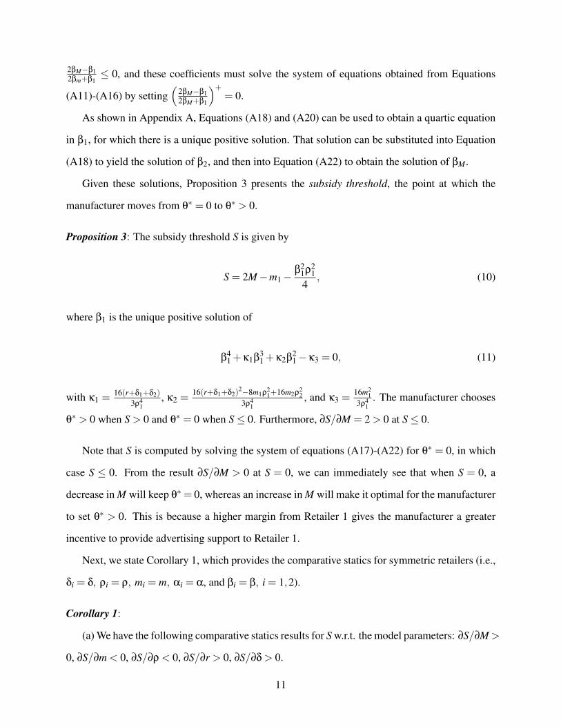
Proposition 3: The subsidy threshold S is given by
S = 2M−m1−β2
1ρ21
4, (10)
where β1 is the unique positive solution of
β41 +κ1β
31 +κ2β
21−κ3 = 0, (11)
with κ1 = 16(r+δ1+δ2)3ρ4
1, κ2 = 16(r+δ1+δ2)
2−8m1ρ21+16m2ρ2
23ρ4
1, and κ3 = 16m2
13ρ4
1. The manufacturer chooses
θ∗ > 0 when S > 0 and θ∗ = 0 when S≤ 0. Furthermore, ∂S/∂M = 2 > 0 at S≤ 0.
Note that S is computed by solving the system of equations (A17)-(A22) for θ∗ = 0, in which
case S ≤ 0. From the result ∂S/∂M > 0 at S = 0, we can immediately see that when S = 0, a
decrease in M will keep θ∗= 0, whereas an increase in M will make it optimal for the manufacturer
to set θ∗ > 0. This is because a higher margin from Retailer 1 gives the manufacturer a greater
incentive to provide advertising support to Retailer 1.
Next, we state Corollary 1, which provides the comparative statics for symmetric retailers (i.e.,
δi = δ, ρi = ρ, mi = m, αi = α, and βi = β, i = 1,2).
Corollary 1:
(a) We have the following comparative statics results for S w.r.t. the model parameters: ∂S/∂M >
0, ∂S/∂m < 0, ∂S/∂ρ < 0, ∂S/∂r > 0, ∂S/∂δ > 0.
11

(b) At the manifold S = 0, we have the following comparative statics results for the model
parameters: ∂M/∂m > 0, ∂ρ/∂m < 0, ∂M/∂δ < 0, ∂m/∂δ > 0, ∂ρ/∂δ > 0, ∂r/∂δ < 0.
The comparative statics in Corollary 1(a) denote the impact of the model parameters on the
subsidy threshold S. The increase of S with respect to M at S = 0 repeats our finding in the
asymmetric case as reported in Proposition 3. Corollary 1(a) also states that the higher the retailers’
margin m is, the lower the manufacturer’s incentive to provide advertising support will be. Since
investments in advertising have a greater impact on a retailer’s profit when margins are high, a
high-margin retailer has its own incentives to invest in advertising. This diminishes the need for
the manufacturer to provide advertising support. A similar argument can be made for the decrease
of S at S ≤ 0 with the retailers’ advertising effectiveness ρ. An increase in the discount rate r or
the decay rate δ, on the other hand, makes it more difficult for a retailer to increase its market
share through advertising. This prompts the manufacturer to provide more advertising support.
Consequently, S increases with r and δ at S≤ 0.
The comparative statics in Corollary 1(b) represent the change needed in one model parameter
to offset a change in another model parameter so as to maintain θ∗= 0. First, consider ∂M/∂m. We
know from Corollary 1(a) that the subsidy threshold S decreases with m. Note also from Corollary
1(a) that S increases with M. Therefore, if m increases (decreases), then M must increase (decrease)
to keep S = 0. If m decreases and M does not, then θ∗ will become strictly positive. Similar effects
can be noted for the impact of δ on m and ρ by looking at the effect of δ, m, and ρ on S in
Corollary 1(a). For ∂M/∂δ, the signs of ∂S/∂M and ∂S/∂δ in Corollary 1(a) can be used to show
that if δ increases (decreases), then M must decrease (increase) to maintain S = 0. Next, consider
the interaction between m and ρ. Since S decreases with both m and ρ, an increase in m has to be
accompanied by a decrease in ρ in order to keep S = 0. For ∂r/∂δ, note that δ works like a discount
rate, as is known in the economics literature. Here, specifically, if r increases by ε, then δ must
decrease by 2ε to keep S = 0.
He et al. (2011) show that when r and δ are small compared to m and M, the subsidy rate
θ∗ > 0 if M > 2m/3. In other words, the manufacturer provides advertising support to Retailer 1
12

operating in a symmetric duopoly if its margin from Retailer 1 exceeds 2m/3. Stated differently,
if m increases by ε, then M must increase by 2ε/3 to maintain S = 0. Let us note that this result
follows also as a corollary of Proposition 3 when the retailers are symmetric and r = δ = 0.
Case θ∗ > 0
When the solution results in S > 0, we know that θ∗ > 0. Then, by substituting(
2βM−β12βM+β1
)+=
2βM−β12βM+β1
into Equations (A11)-(A16), we have the following system of equations to solve for the
value-function coefficients:
rα1 =18
β1ρ21(2βM +β1)+β1δ2, (12)
rβ1 = m1−18
β1ρ21(2βM +β1)−
12
β1β2ρ22−β1 (δ1 +δ2) , (13)
rα2 =14
β22ρ
22 +β2δ1, (14)
rβ2 = m2−14
β2ρ21(2βM +β1)−
14
β22ρ
22−β2 (δ1 +δ2) , (15)
rαM =1
16ρ
21(2βM +β1)2 +βMδ2, (16)
rβM = M− 116
ρ21(2βM +β1)2− 1
2β2βMρ
22−βM (δ1 +δ2) . (17)
This requires numerical analysis. Figure 2 illustrates the effect of the retailer’s margin on the
manufacturer’s subsidy rate for the following sample parameter values: r = 0.03, ρ1 = ρ2 = 0.5,
δ1 = 0.07, δ2 = 0.1, M = 0.5. Furthermore, for the effect of Retailer 1’s (Retailer 2’s) margin, we
set m2 = 0.5 (m1 = 0.5).
——————————–
Insert Figure 2 here.
——————————–
We already know from Corollary 1(a) that ∂S/∂m < 0 at S≤ 0 in the symmetric case. The result
shown in Figure 2—that θ∗ decreases, and at a decreasing rate, as the margin m1 increases—is con-
sistent with our finding in the symmetric case and represents its generalization to the asymmetric
13

case. The reason is that with low margin m1, Retailer 1 will under-advertise and the manufacturer’s
profit will suffer on account of decreased sales. So, then, it is in the interest of the manufacturer to
provide a subsidy to encourage the retailer to advertise more. As m1 increases, Retailer 1 has its
own incentive to advertise, and therefore the manufacturer does not need to offer as much in the
way of a subsidy. As m1 keeps increasing, the manufacturer ceases to participate altogether. We
see from Figure 2 that θ∗ indeed becomes zero at m1 ≈ 0.8, where the switch from “cooperative
advertising” to “no cooperative advertising” takes place. This generalizes the result obtained in He
et al. (2009) in the absence of competition, to the competitive environment.
The effect of the margin of the non-supported retailer (i.e. Retailer 2) on the offer of coop-
erative advertising to Retailer 1, appears to be weak. Note that at m1 = 0.5, the two curves in
Figure 2 cross. At this point, as m1 increases, ceteris paribus, θ∗ decreases sharply whereas as m2
increases, θ∗ increases slowly. This means that as m2 increases, Retailer 1 faces greater advertising
competition from the competing retailer, and this induces the manufacturer to support Retailer 1
at a slightly higher rate. On the other hand, as m1 increases, as has already been mentioned, it in-
creases the incentive of Retailer 1 to advertise of its own accord and thus the manufacturer reduces
its support significantly. Even though m2 has a weak effect on θ∗, it may still make a difference
between the manufacturer supporting or not supporting Retailer 1. Numerical analysis shows that
when m1 = m2 = 0.5, then θ∗ = 0.278. However, as m2 decreases from 0.5 (e.g., m2 = 0.2) the
manufacturer stops offering advertising support to Retailer 1. On the other hand, as m2 increases
from 0.5 to 0.8, θ∗ increases only marginally from a support of 27.8% to 29.1%.
——————————–
Insert Figure 3 here.
——————————–
In Figure 3, the fixed parameter values are: m1 = 0.2, m2 = 0.5, r = 0.03, δ1 = 0.07, δ2 = 0.1,
M = 0.5. To find the effect of Retailer 1’s (Retailer 2’s) advertising effectiveness, we set ρ2 = 0.5
(ρ1 = 0.5). Consistent with the comparative statics result for the symmetric case in Corollary 1(a)
(that ∂S/∂ρ < 0), this figure shows that as the advertising effectiveness of Retailer 1 increases, the
14

degree of support by the manufacturer diminishes. The reason is that given the greater effectiveness
of advertising, the retailer has an incentive to advertise at a higher level even without the support
of the manufacturer. Retailer 2’s advertising effectiveness does not have a great impact, but as it
increases it slowly raises the subsidy rate.
——————————–
Insert Figure 4 here.
——————————–
Finally, Figure 4 shows that as the sum of the market share decay rates for the two retailers
increases, the subsidy rate to Retailer 1 increases. For this figure, the remaining parameter values
are: m1 = 0.5, m2 = 0.2, r = 0.03, ρ1 = 0.5, ρ2 = 0.5, M = 0.8. Note that we have plotted θ∗
against the sum of the decay rates since it is clear from the dynamics in Equation (1) that the decay
rate for Retailer 1 is (δ1 +δ2). It is for this reason that we can easily see from Equations (12)-(17)
that β1, β2, and βM, and, therefore, θ∗, are affected by the sum (δ1 +δ2) and not by the individual
decay rates. The result can be explained intuitively since the increase of (δ1 + δ2) is similar to
increasing the speed of the treadmill with which the advertising must keep up. Thus, as (δ1 + δ2)
increases, Retailer 1 finds it more expensive to maintain its market share and the manufacturer must
offer a higher subsidy rate to Retailer 1 to adequately promote the product. This finding generalizes
to the asymmetric case the analytical result obtained for the symmetric case in Corollary 1(a), that
∂S/∂δ > 0. Finally, note that the effect of the decay rates is most pronounced at their lower values
and the decay rates do not have much effect on the subsidy rate at higher values.
OLIGOPOLY RETAIL MARKET
We are interested in examining the impact of retail competition on the optimal subsidy rate. To that
end, we consider an oligopoly in which Retailer 1 has n−1 outside competitors. For tractability,
we focus on the case of n symmetric retailers, where mi = m, ρi = ρ, δi = δ for i ∈ {1,2, ...n}. As
before, the manufacturer offers a cooperative advertising subsidy only to Retailer 1.
15

The demand dynamics generalizes the duopoly specification as follows:
xi(t) =n
n−1ρui√
1− xi−1
n−1
n
∑j=1
ρu j√
1− x j−δ
(xi−
1n
), xi(0) = xi0, i ∈ {1,2, ...,n}.
(18)
The first term captures the gain in market share from the competitors, the second term the loss
of market share to the competitors, and the third term the market share churn. This model of retail
competition is discussed and validated in Prasad et al. (2009). It should be noted that with more
than three retailer types there is the possibility that market shares can go out-of-bounds, referring
to Naik et al. (2008) for this type of dynamics. By assuming that the competing retailers are
all homogenous with each other, though not necessarily with the focal retailer, we side-step the
out-of-bounds problem while allowing for any number of retailers.
Since ∑ni=1 xi = 1, the differential game is properly formulated with n− 1 independent states,
which we choose to be x2, x3, ...,xn. Each retailer maximizes its profit with respect to its advertising
decision given the subsidy rate θ(x2,x3, ...,xn) announced by the manufacturer. The objective
functions of the n retailers are given by
V1(x20,x30, ...,xn0) = maxu1(t), t≥0
∫∞
0e−rt
(m(1−
n
∑i=2
xi (t))− ((1−θ(x2(t),x3(t), ...,xn(t)))u21(t)
)dt,
(19)
Vi(x20,x30, ...,xn0) = maxui(t), t≥0
∫∞
0e−rt (mxi(t)−u2
i (t))
dt, i ∈ {2,3, ...,n}, (20)
subject to Equation (18).
The manufacturer’s objective function, with a slight abuse of notation, is
V (x20,x30, ...,xn0) = maxθ(t), t≥0
∫∞
0e−rt
(M(1−
n
∑i=2
xi (t))−θ(t)u21(t)
)dt, (21)
subject to Equation (18).
16

Proposition 4: The feedback Stackelberg equilibrium with n symmetric retailers is characterized
as follows:
(a) The optimal advertising decisions of the retailers are given by
u1(x2,x3, ...,xn|θ) =−ρ
√∑
nj=2 x j
2(n−1)(1−θ)
(n
∑k=2
∂V1
∂xk
), (22)
ui(x2,x3, ...,xn|θ) =ρ√
1− xi
2(n−1)
(n
∂Vi
∂xi−
n
∑k=2
∂Vi
∂xk
), i ∈ {2,3, ...,n}. (23)
(b) The optimal subsidy rate of the manufacturer has the form
θ(x2,x3, ...,xn) =(
2B−A2B+A
)+
, (24)
where A = ∑nj=2
∂V1∂x j
and B = ∑nj=2
∂V∂x j
.
(c) The value functions Vi for Retailer i, i = 1,2, ...,n, and V for the manufacturer, satisfy the
n+1 Equations (A31)-(A33) in Appendix A.
As before, we look for the linear value functions Vi, i ∈ {1,2, ...,n}. To obtain their forms, we
proceed as follows. Note that when θ = 0, the n retailers simply play a Nash game. Since they are
symmetric when θ = 0, it is convenient to visualize the linear value function forms in terms of x1,
x2, ..., xn. Thus,
V1 = α+βx1 + γx2 + γx3 + ...+ γxn,
V2 = α+ γx1 +βx2 + γx3 + ...+ γxn,
V3 = α+ γx1 + γx2 +βx3 + ...+ γxn,
...
Vn = α+ γx1 + γx2 + γx3 + ...+βxn.
Note that the above specification can have non-unique coefficients on account of a redundant state,
17

but they would express the same value function. For example, we can write V1 in the following
two ways:
V1 = α+β
2x1 +
β
2
(1−
n
∑i=2
xi
)+ γx2 + γx3 + ...+ γxn
=(
α+β
2
)+
β
2x1 +
(γ− β
2
)x2 +
(γ− β
2
)x3 + ...+
(γ− β
2
)xn.
In order to obtain the value functions in terms of x2, x3, ..., xn, we replace x1 by (1−∑ni=2 xi) to
obtain
V1 = (α+β)− (β− γ)n
∑i=2
xi,
V2 = (α+ γ)+(β− γ)x2,
V3 = (α+ γ)+(β− γ)x3,
...
Vn = (α+ γ)+(β− γ)xn.
Let α+β = a and β− γ = b. Then, α+ γ = a−b, and we have
V1 = a−bn
∑j=2
x j, Vi = (a−b)+bxi, i = 2,3, ...n. (25)
We should note that the form of Equation (25) will have unique coefficients.
Similarly, for the case when θ > 0, we can write the value functions for the manufacturer and
the retailers as: V = P−Q(∑ni=2 xi), V1 = a1−b1(∑n
i=2 xi), Vi = (a−b)+bxi, i = 2,3, ...,n, where a,
b, a1, b1, P, and Q are constants. Note that when θ > 0, Retailers i, for i = 2,3, ...,n, are symmetric
but Retailer 1 changes when it gets a subsidy. Therefore, the coefficients a1 6= a and b1 6= b when
θ > 0. The results of the case when θ > 0 are summarized in Proposition 4.
Proposition 5:
18
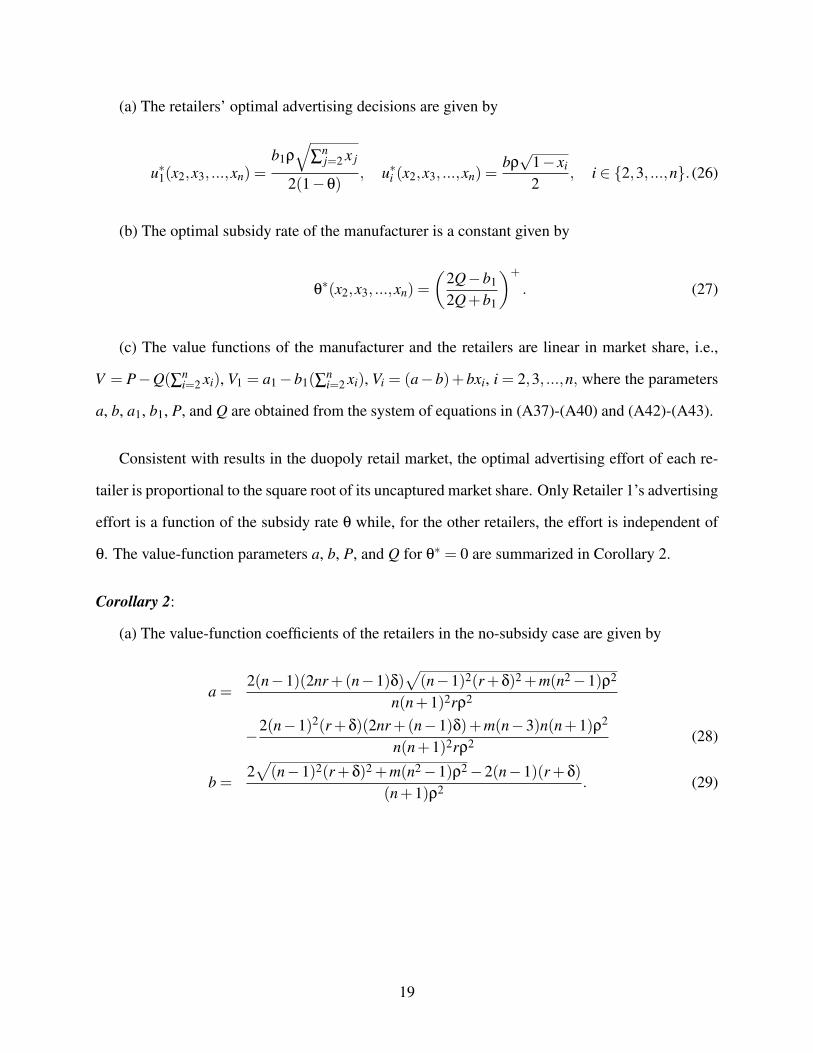
(a) The retailers’ optimal advertising decisions are given by
u∗1(x2,x3, ...,xn) =b1ρ
√∑
nj=2 x j
2(1−θ), u∗i (x2,x3, ...,xn) =
bρ√
1− xi
2, i ∈ {2,3, ...,n}. (26)
(b) The optimal subsidy rate of the manufacturer is a constant given by
θ∗(x2,x3, ...,xn) =
(2Q−b1
2Q+b1
)+
. (27)
(c) The value functions of the manufacturer and the retailers are linear in market share, i.e.,
V = P−Q(∑ni=2 xi), V1 = a1−b1(∑n
i=2 xi), Vi = (a−b)+bxi, i = 2,3, ...,n, where the parameters
a, b, a1, b1, P, and Q are obtained from the system of equations in (A37)-(A40) and (A42)-(A43).
Consistent with results in the duopoly retail market, the optimal advertising effort of each re-
tailer is proportional to the square root of its uncaptured market share. Only Retailer 1’s advertising
effort is a function of the subsidy rate θ while, for the other retailers, the effort is independent of
θ. The value-function parameters a, b, P, and Q for θ∗ = 0 are summarized in Corollary 2.
Corollary 2:
(a) The value-function coefficients of the retailers in the no-subsidy case are given by
a =2(n−1)(2nr +(n−1)δ)
√(n−1)2(r +δ)2 +m(n2−1)ρ2
n(n+1)2rρ2
−2(n−1)2(r +δ)(2nr +(n−1)δ)+m(n−3)n(n+1)ρ2
n(n+1)2rρ2 (28)
b =2√
(n−1)2(r +δ)2 +m(n2−1)ρ2−2(n−1)(r +δ)(n+1)ρ2 . (29)
19

(b) The value-function coefficients of the manufacturer in the no-subsidy case are given by
P =2M(
4δ−3(√
(r +δ)2 +2mρ2− r−δ
))3(
r +δ+3√
(r +δ)2 +2mρ2) (30)
Q =M(n2−1)
(n−1)(r +δ)+n√
(n−1)2(r +δ)2 +m(n2−1)ρ2. (31)
The subsidy threshold S is presented in Proposition 6.
Proposition 6: The subsidy threshold S in the case of n symmetric retailers is given by
S =2Qb−1, (32)
where b and Q are given by Equations (29) and (31), respectively.
When r = δ = 0, the subsidy threshold in Equation (32) reduces to a simpler form as shown
below.
Corollary 3: When r = δ = 0, the expression for S in Equation (32) reduces to
S =(n+1)M−nm
nm. (33)
From Corollary 3, we can see that θ > 0 if M > ( nn+1)m. That is, the manufacturer provides
cooperative advertising support to Retailer 1 if its margin M is greater than nn+1 times the retailer’s
margin m. We now compare this result to those in the cases of a duopoly retail market and a
monopolist retailer.
20

Comparison of the Three Market Structures: Monopoly, Duopoly, and
Oligopoly
We now examine the role of competition by comparing the optimal subsidy threshold in the retail
duopoly and oligopoly cases to those in He et al. (2009) for a retail monopolist. He et al. (2009)
show that when r and δ are small, the manufacturer subsidizes the retailer when M > m. Without
a subsidy, the convex advertising cost and the shrinking market potential dissuade the monopolist
retailer from advertising enough to capture the market potential that is beneficial to the manufac-
turer.
In a retail duopoly, the manufacturer subsidizes Retailer 1 when M > 2m/3. For n retailers,
the manufacturer subsidizes Retailer 1 when M > ( nn+1)m. In the limit, as n approaches ∞, the
previous inequality reverts back to M > m, which is the same as that for a retail monopolist.
In other words, compared to the case of a monopolist retailer, the manufacturer provides sup-
port under a wider range of conditions when its retailer competes in a duopoly. But the range of
support decreases monotonically (while always remaining higher than in the monopoly case) as
the number of competitors increases from 2 to ∞, converging to the monopoly result as n→ ∞.
The numerical results suggest that this pattern of responses to the number of competitors, in-
creasing and then retreating to the monopoly baseline, does not occur just for the subsidy threshold,
but for the subsidy rate as well, including over the range of parameter values with r > 0 and δ > 0.
However, this pattern could only be proved for r = δ = 0. For example, Figure 5 provides subsidy
rates in monopoly, duopoly, and oligopoly as a function of the manufacturer’s margin M. The
fixed parameter values are m = 0.5, r = 0.03, ρ = 0.5, and δ = 0.1. Furthermore, θ∗NC denotes the
optimal subsidy rate in the absence of retail competition, θ∗D denotes the optimal subsidy rate in a
retail duopoly, and θ∗T that in a retail triopoly.
——————————–
Insert Figure 5 here.
——————————–
21

From the figure, the threshold value of M at which the manufacturer supports its retailer in the
presence of competition is lower than that without competition. In particular, the manufacturer
begins setting θ∗D > 0 when M increases to about 0.3 and θ∗T > 0 when M increases to about
0.33, compared to θ∗NC > 0 when M ≈ 0.38. In other words, the manufacturer provides cooperative
advertising support for a wider range of model parameters in the duopoly case than in the monopoly
case, and the support range in the triopoly case lies between the cases of monopoly and duopoly.
As is clear from Figure 5, a wider range of support is also associated with a higher level of support
for every value of M larger than the threshold value where subsidy becomes positive. Finally, we
see from the figure that while the subsidy rate under competition is higher than that in the absence
of competition, the difference in subsidy rate declines as M increases.
The intuitive interpretation is as follows. First, when we move from a monopoly to a duopoly,
Retailer 1 finds itself in competition with Retailer 2. Since Retailer 2’s advertising effort is directed
to wrest market share from Retailer 1, thereby hurting the manufacturer’s profit, the manufacturer’s
support for Retailer 1 is higher in the presence of competing Retailer 2 than in its absence.
This implies that there is an effect, which we refer to as the primary effect, whereby the man-
ufacturer will increase support so that its retailer will win or retain some share in a competitive
market. However, if this was the only effect, we would expect the support to keep increasing as
more competitors entered the market. But as the number of competitors increases, an interesting
reversal occurs. Let us consider a triopoly with an additional Retailer 3. Now we find that the
manufacturer’s support to its retailer in a triopoly continues to be higher than that in monopoly, but
lower than that in duopoly. This suggests a secondary effect of competitive entry.
The reason for this behavior appears to be that the competition between outside Retailers 2 and
3 creates an added incentive for Retailer 1 to advertise on its own accord, so the manufacturer does
not need to support Retailer 1 in a triopoly as much as it would in a duopoly. But this secondary
effect of free-riding does not dominate the primary effect, so as a result the triopoly support is
still greater than in a monopoly case. Moreover, as n increases, the secondary effect increases
monotonically so that support continues to decrease. However, support remains higher than in a
22

monopoly as indicated by the fact that the support threshold converges to the monopoly level as
n→ ∞.
Before concluding this section, we should recapitulate that those effects that were seen in
the absence of competition also hold under competition. First, the result that the subsidy rate
declines with higher retailer margin continues to hold under competition, and the intuition is that
less incentive is needed since the retailer’s interest in increasing market share is more closely
aligned with that of the manufacturer. Second, we find that as Retailer 2’s margin increases, the
manufacturer offers more support to Retailer 1. The intuition behind this is that because Retailer 2
with a higher margin is a fiercer competitor, the manufacturer’s support for Retailer 1 is higher to
encourage that retailer to advertise more to counter the effect of the competition.
CONCLUSIONS
In this paper, we consider a consumer goods manufacturer who sells through a retailer in compe-
tition with outside retailers. The retailers invest in local advertising effort, while the manufacturer
decides whether or not to support its retailer’s advertising activities by providing a subsidy rate.
We model the interaction between the manufacturer and its retailer as a Stackelberg differential
game and the interaction between the competing retailers as a Nash differential game.
We derive the optimal feedback advertising effort levels of the retailers and the feedback sub-
sidy rate of the manufacturer. Compared to He et al. (2009), who do not model retail competition,
we find that in a retail duopoly the presence of a competing retailer induces the manufacturer
to provide a higher level of cooperative advertising support to its retailer over a greater range of
parameter values, than if that retailer were a monopolist. Interestingly, the manufacturer provides
lower levels of advertising support as the intensity of competition increases, and in the limit, we ob-
tain the monopoly result. This is because an increase in outside competition induces the supported
retailer to advertise heavily of its own accord in order to wrest market share from its competing
retailers, thus giving a free ride to the manufacturer.
23

Appendix B provides a brief discussion of two extensions. In the first, we consider the case
where the manufacturer has the choice of selling through all of the retailers, and therefore has an
option of supporting some or all of them. We show that when retailers are symmetric and one
retailer provides a higher margin to the manufacturer than the others providing equal margins, then
the manufacturer supports only the dominant retailer. It would be of interest to extend this analysis
to asymmetric retailers. In the second extension, we incorporate retail price competition in the
model. We did not consider the manufacturers wholesale price decision as in He et al. (2009) in
the case of a single-manufacturer, single-retailer channel. Future research could examine the role
of the wholesale price as another instrument for the manufacturer.
This paper also opens up a fruitful avenue for empirical research. Given the expression for
the optimal subsidy rate as a function of various firm- and industry-level parameters, one could
empirically examine whether our results can explain the differences in the subsidy rates in dif-
ferent industries as reported in Dutta et al. (1995). This would require estimation of the firm-
and industry-level parameters, possibly employing the techniques used in Naik et al. (2008). Pro-
vided an appropriate data set can be found or collected, an empirical study to validate our results
would undoubtedly deepen our understanding of the cooperative advertising practices in different
industries.
REFERENCES
Bass, F. M., Krishnamoorthy, A., Prasad, A., & Sethi, S. P. (2005). Generic and brand advertising
strategies in a dynamic duopoly. Marketing Science, 24(4), 556-568.
Bergen, M., & John, G. (1997). Understanding cooperative advertising participation rates in
conventional channels. Journal of Marketing Research, 34(2), 357-369.
Berger, P. D. (1972). Vertical cooperative advertising ventures. Journal of Marketing Research,
9(3), 309-312.
24

Berger, P. D., & Magliozzi, T. (1992). Optimal cooperative advertising decisions in direct-mail
operations. Journal of the Operational Research Society, 43(11), 1079-1086.
Chintagunta, P. K., & Jain, D. C. (1992). A dynamic model of channel member strategies for
marketing expenditures. Marketing Science, 11(2), 168-188.
Chintagunta, P. K., & Jain, D. C. (1995). Empirical analysis of a dynamic duopoly model of
competition. Journal of Economics & Management Strategy, 4(1), 109-131.
Chintagunta, P. K., & Vilcassim, N. J. (1992). An empirical investigation of advertising strategies
in a dynamic duopoly. Management Science, 38(9), 1230-1244.
Dant, R. P., & Berger, P.D. (1996). Modeling cooperative advertising decisions in franchising.
Journal of the Operational Research Society, 47(9), 1120-1136.
Deal, K. R. (1979). Optimizing advertising expenditures in a dynamic duopoly. Operations
Research, 27(4), 682-692.
Dutta, S., Bergen, M., John, G., & Rao, A. (1995). Variations in the contractual terms of cooper-
ative advertising contracts: An empirical investigation. Marketing Letters, 6(1), 15-22.
Erickson, G. M. (1992). Empirical analysis of closed-loop duopoly advertising strategies. Man-
agement Science, 38(12), 1732-1749.
Erickson, G. M. (2009a). An oligopoly model of dynamic advertising competition. European
Journal of Operational Research, 197(1), 374-388.
Erickson, G. M. (2009b). Advertising competition in a dynamic oligopoly with multiple brands.
Operations Research, 57(5), 1106-1113.
Feichtinger, G., Hartl, R. F., & Sethi, S. P. (1994). Dynamic optimal control models in advertising:
Recent developments. Management Science, 40(2), 195-226.
25

Fruchter, G. E., & Kalish, S. (1997). Closed-loop advertising strategies in a duopoly. Manage-
ment Science, 43(1), 54-63.
He, X., Krishnamoorthy, A., Prasad, A., & Sethi, S. P. (2011). Retail competition and cooperative
advertising. Operations Research Letters, 39(1), 11-16.
He, X., Prasad, A., & Sethi, S. P. (2009). Cooperative advertising and pricing in a dynamic
stochastic supply chain: Feedback Stackelberg strategies. Production and Operations Man-
agement, 18(1), 78-94.
He, X., Prasad, A., Sethi, S. P., & Gutierrez, G. J. (2007). A survey of Stackelberg differential
game models in supply and marketing channels. Journal of Systems Science and Systems
Engineering, 16(4), 385-413.
Huang, Z., Li, S. X., & Mahajan, V. (2002). An analysis of manufacturer-retailer supply chain
coordination in cooperative advertising. Decision Sciences, 33(3), 469-494.
Jørgensen, S., Sigue, S. P., & Zaccour, G. (2000). Dynamic cooperative advertising in a channel.
Journal of Retailing, 76(1), 71-92.
Jørgensen, S., Taboubi, S., & Zaccour, G. (2001). Cooperative advertising in a marketing channel.
Journal of Optimization Theory and Applications, 110(1), 145-158.
Jørgensen, S., Taboubi, S., & Zaccour, G. (2003). Retail promotions with negative brand image
effects: Is cooperation possible? European Journal of Operational Research, 150(2), 395-
405.
Jørgensen, S., & Zaccour, G. (2003). Channel coordination over time: Incentive equilibria and
credibility. Journal of Economic Dynamics and Control, 27(5), 801-822.
Kali, R. (1998). Minimum advertised price. Journal of Economics and Management Strategy,
7(4), 647-668.
26

Karray, S., & Zaccour, G. (2005). A differential game of advertising for national brand and store
brands. In A. Haurie, & G. Zaccour (Eds.), Dynamic Games: Theory and Applications. New
York: Springer, 213-229.
Kim, S. Y., & Staelin, R. (1999). Manufacturer allowances and retailer pass-through rates in a
competitive environment. Marketing Science, 18(1), 59-76.
Naik, P. A., Prasad, A., & Sethi, S. P. (2008). Building brand awareness in dynamic oligopoly
markets. Management Science, 54(1), 129-138.
Prasad, A., & Sethi, S. P. (2004). Competitive advertising under uncertainty: A stochastic differ-
ential game approach. Journal of Optimization Theory and Applications, 123(1), 163-185.
Prasad, A., Sethi, S. P., & Naik, P. A. (2009). Optimal control of a dynamic oligopoly model
of advertising. In Proceedings of the 13th IFAC Symposium on Information Control Prob-
lems in Manufacturing, INCOM 2009, Moscow, Russia. Laxenburg, Austria: International
Federation of Automatic Control.
Sethi, S. P. (1977). Dynamic optimal control models in advertising: A survey. SIAM Review,
19(4), 685-725.
Sethi, S. P. (1983). Deterministic and stochastic optimization of a dynamic advertising model.
Optimal Control Applications and Methods, 4(2), 179-184.
Sorger, G. (1989). Competitive dynamic advertising: A modification of the Case game. Journal
of Economic Dynamics and Control, 13(1), 55-80.
27

APPENDIX A
Proof of Proposition 1
The Hamilton-Jacobi-Bellman (HJB) equation for Retailer i is given by
rV1 = maxu1
{m1x− (1−θ)u2
1 +V′1
(ρ1u1√
1− x−ρ2u2√
x−δ1x+δ2 (1− x))}
, (A1)
rV2 = maxu2
{m2(1− x)− (1−θ2)u2
2 +V′2
(ρ1u1√
1− x−ρ2u2√
x−δ1x+δ2 (1− x))}
. (A2)
The first-order conditions for maximization yield the optimal advertising levels in Equation (6) in
Proposition 1(a). Substituting these solutions into the above HJB equations for the two retailers
yields the following two equations:
rV1 = m1x+ρ2
1
(V′1
)2
4
(1−(
2V ′−V ′12V ′+V ′1
)+) (1− x)+
V′1V′2ρ2
22
x−V′1 (δ1x−δ2 (1− x)) , (A3)
rV2 = m2 (1− x)+ρ2
2
(V′2
)2
4x+
V′1V′2ρ2
1
2
(1−(
2V ′−V ′12V ′+V ′1
)+) (1− x)−V
′2 (δ1x−δ2 (1− x)) , (A4)
The HJB equation for the manufacturer is given by
rV = maxθ
{Mx−θu2
1 (x|θ)+V′(
ρ1u1 (x|θ)√
1− x−ρ2u2 (x|θ)√
x−δ1x+δ2 (1− x))}
. (A5)
Substituting the optimal advertising efforts of the two retailers into the above equation and simpli-
fying yields
rV = maxθ
Mx−θρ2
1
(V′1
)2(1− x)
4(1−θ)2 +V′
(ρ2
1V′1(1− x)
2(1−θ)+
ρ22V′2x
2−δ1x+δ2(1− x)
) . (A6)
Solving the first-order conditions for the subsidy rates yields Equation (7) in Proposition 1(b).
28

Substituting these solutions into Equation (A6) and simplifying, we obtain the following equation
for the manufacturer:
rV = Mx−ρ2
1
(V′1
)2(
2V′−V
′1
2V ′+V ′1
)+
(1− x)
4
((1− 2V ′−V ′1
2V ′+V ′1
)+)2
+V′V′2ρ2
2x2
−V′V′1ρ2
1(1− x)
2
((1− 2V ′−V ′1
2V ′+V ′1
)+) −δ1V
′x+δ2V
′(1− x). � (A7)
Proof of Proposition 2
With V1 = α1 +β1x and V2 = α2 +β2 (1− x), we have V′1 = β1 and V
′2 =−β2. Inserting these into
Equations (A3) and (A4), we have
r (α1 +β1x) = m1x+β2
1ρ21 (1− x)
4(
1−(
2V ′−β12V ′+β1
)+) − β1β2ρ2
2x2
−β1 (δ1x−δ2 (1− x)) , (A8)
r (α2 +β2 (1− x)) = m2 (1− x)+β2
2ρ22x
4−
β1β2ρ21 (1− x)
2(
1−(
2V ′−β12V ′+β1
)+) +β2 (δ1x−δ2 (1− x)) . (A9)
With V = αM +βMx, we have V′= βM. Substitution into Equations (6) and (7) yields Equation (8)
in Proposition 2(a) and Equation (9) in Proposition 2(b), respectively. Substituting these into the
HJB equation (A7) and simplifying, we have
r (αM +βMx) = Mx−β2
1ρ21
(2βM−β12βM+β1
)+(1− x)
4(
1−(
2βM−β12βM+β1
)+)2 −
β2βMρ22x
2
+β1βMρ2
1(1− x)
2(
1−(
2βM−β12βM+β1
)+) −δ1βMx+δ2βM(1− x). (A10)
29

The system of equations to solve for the six value-function coefficients in Proposition 2(c) are
rα1 =β2
1ρ21
4(
1−(
2βM−β12βM+β1
)+) +β1δ2, (A11)
rβ1 = m1−β2
1ρ21
4(
1−(
2βM−β12βM+β1
)+) − β1β2ρ2
22−β1 (δ1 +δ2) , (A12)
rα2 =β2
2ρ22
4+β2δ1, (A13)
rβ2 = m2−β2
2ρ22
4−
β1β2ρ21
2(
1−(
2βM−β12βM+β1
)+) −β2 (δ1 +δ2) , (A14)
rαM =−β2
1ρ21
(2βM−β12βM+β1
)+
4(
1−(
2βM−β12βM+β1
)+)2 +
β1βMρ21
2(
1−(
2βM−β12βM+β1
)+) +δ2βM, (A15)
rβM = M +β2
1ρ21
(2βM−β12βM+β1
)+
4(
1−(
2βM−β12βM+β1
)+)2 −
β2βMρ22
2−
β1βMρ21
2(
1−(
2βM−β12βM+β1
)+) − (δ1 +δ2)βM. (A16)
We obtain these by substituting V′= βM into Equations (A8)-(A9) and equating the powers of x
and (1− x) in Equations (A8)-(A10). �
30

Proof of Proposition 3
Setting(
2βM−β12βM+β1
)+= 0, we have:
rα1 =β2
1ρ21
4+β1δ2, (A17)
rβ1 = m1−β2
1ρ21
4−
β1β2ρ22
2−β1 (δ1 +δ2) , (A18)
rα2 =β2
2ρ22
4+β2δ1, (A19)
rβ2 = m2−β2
2ρ22
4−
β1β2ρ21
2−β2 (δ1 +δ2) , (A20)
rαM =12
β1βMρ21 +βMδ2, (A21)
rβM = M− 12
β1βMρ21−
12
β2βMρ22−βM (δ1 +δ2) . (A22)
Solving Equation (A18) for β2 yields
β2 =4m1−β1
(β1ρ2
1 +4(r +δ1 +δ2))
2β1ρ22
. (A23)
Substituting the above solution into Equation (A20) and simplifying yields the quartic Equation
(11). As detailed in Prasad and Sethi (2004), it can be shown that there exists a unique β1 > 0 that
solves the above quartic equation. This is the unique equilibrium of the Stackelberg differential
game. That solution can then be substituted into Equation (A23) to obtain the solution for β2. We
know from Equation (A22) that
βM =2M
β1ρ21 +β2ρ2
2 +2(r +δ1 +δ2). (A24)
Substituting the solutions for β1 and β2 into Equation (A24) yields βM. Since βM > 0 from Equa-
tion (A16), the subsidy threshold is obtained as 2βM−β1. We have
4Mβ1ρ2
1 +β2ρ22 +2(r +δ1 +δ2)
−β1 =4M−β2
1ρ21−β1β2ρ2
2−2β1 (r +δ1 +δ2)β1ρ2
1 +β2ρ22 +2(r +δ1 +δ2)
. (A25)
31

We know from Equation (A18) that
β1β2ρ22 +2β1 (δ1 +δ2) =
12(4m1−4rβ1−β
21ρ
21).
Using this in the numerator of Equation (A25) and simplifying gives the subsidy threshold S in
Equation (10). Since β1 is independent of M, we have ∂S/∂M = 2 > 0. �
Proof of Corollary 1
The solutions for the value-function coefficients can be found in He et al. (2011). For the
comparative statics, imposing symmetry in the subsidy threshold from Equation (10), we have
S(·) = 2M−m− β2ρ2
4 = 0. In this threshold, we substitute the solution for β, as specified in He et
al. (2011) to obtain
S(·) = 2M− 43
m+2(r +2δ)
(√(r +2δ)2 +3mρ2− (r +2δ)
)9ρ2 . (A26)
Taking the derivative of S in Equation (A26) w.r.t. the model parameters yields the compar-
ative statics in Corollary 1(a): ∂S/∂M = 2 > 0, ∂S/∂m = r+2δ
3√
(r+2δ)2+3mρ2− 4
3 < 0, ∂S/∂ρ =
2m(r+2δ)3ρ
√(r+2δ)2+3mρ2
−4(r+2δ)
(√(r+2δ)2+3mρ2−r−2δ
)9ρ3 < 0, ∂S/∂r =
2(√
(r+2δ)2+3mρ2−r−2δ
)2
9ρ2√
(r+2δ)2+3mρ2> 0, and
∂S/∂δ =4(√
(r+2δ)2+3mρ2−r−2δ
)2
9ρ2√
(r+2δ)2+3mρ2> 0.
For any two parameters ψ and χ, the implicit function theorem yields sign[∂ψ/∂χ] =
sign[− ∂S/∂χ
∂S/∂ψ]. Thus, − ∂S/∂m
∂S/∂(M) = 12
(43 −
r+2δ
3√
(r+2δ)2+3mρ2
)> 0,
−∂S/∂m∂S/∂ρ
=−3ρ3(
4√
(r+2δ)2+3mρ2)−(r+2δ)
2(r+2δ)(
3mρ2−2(r+2δ)(√
(r+2δ)2+3mρ2)−(r+2δ)
) < 0,
− ∂S/∂δ
∂S/∂M = −2(√
(r+2δ)2+3mρ2−(r+2δ))2
9ρ2√
(r+2δ)2+3mρ2< 0, − ∂S/∂δ
∂S/∂m =4(√
(r+2δ)2+3mρ2−(r+2δ))2
3ρ2(
4√
(r+2δ)2+3mρ2−(r+2δ)) > 0, − ∂S/∂δ
∂S/∂ρ=
2ρ
r+2δ> 0, and −∂S/∂δ
∂S/∂r =−2 < 0. The comparative statics results in Corollary 1(b) follow. �
32

Proof of Proposition 4
The HJB equation for Retailer 1 is given by
rV1 = maxu1
m(
1−∑nj=2 x j
)− (1−θ)u2
1
+∑nj=2
∂V1∂x j
( nρ
n−1u j√
1− x j− 1n−1 ∑
nk=1 ρuk
√1− xk−δ
(x j− 1
n
)).
(A27)
The HJB equation for Retailer i, i ∈ {2,3, ...,n}, is given by
rVi = maxu1
{mxi−u2
i +∑nj=2
∂Vi∂x j
( nρ
n−1u j√
1− x j− 1n−1 ∑
nk=1 ρuk
√1− xk−δ
(x j− 1
n
)). (A28)
The first-order conditions for maximization yield the optimal advertising levels in Equations
(22)-(23) in Proposition 4(a). The HJB equation for the manufacturer is given by
rV = maxθ(t)
M(1−∑
nj=2 x j)−θu2
1
+∑nj=2
∂V∂x j
( nn−1ρu j
√1− x j− 1
n−1 ∑nk=2 ρuk
√1− xk−δ
(x j− 1
n
)).
(A29)
Substituting the optimal advertising efforts of the n retailers, specified in Equations (22)-(23),
into Equation (A29) and simplifying yields
rV = maxθ(t)
M(1−∑
nj=2 x j)−
θρ2∑
nj=2 x j
4(n−1)2(1−θ)2
(∑
nk=2
∂V1∂xk
)2
+ρ2
∑nj=2 x j
2(n−1)2(1−θ)
(∑
nk=2
∂V1∂xk
)(∑
nj=2
∂V∂x j
)+∑
nj=2
ρ2(1−x j)2(n−1)2
(n ∂V
∂x j−∑
nk=2
∂V∂xk
)(n∂V j
∂x j−∑
nk=2
∂V j∂xk
)−∑
nj=2
∂V∂x j
δ(x j− 1
n
).
(A30)
Using the first-order condition of Equation (A30) w.r.t. θ and simplifying yields Proposition
4(b). Substituting Equations (22)-(24) into Equations (A27)-(A28) and (A30) yields the following
simultaneous equations satisfied by the value functions Vi for Retailer i, i = 1,2, ...,n, and V for
the manufacturer:
33

rV1 = m
(1−
n
∑j=2
x j
)+
ρ2∑
nj=2 x j
4(n−1)2(
1−(2B−A
2B+A
)+)(
n
∑k=2
∂V1
∂xk
)2
+n
∑j=2
ρ2(1− x j)2(n−1)2
(n
∂V1
∂x j−
n
∑k=2
∂V1
∂xk
)(n
∂Vj
∂x j−
n
∑k=2
∂Vj
∂xk
)−
n
∑j=2
∂V1
∂x jδ
(x j−
1n
). (A31)
rVi = mxi +ρ2(1− xi)4(n−1)2
(n
∂Vi
∂xi−
n
∑k=2
∂Vi
∂xk
)2
+ρ2
∑nj=2 x j
2(n−1)2(
1−(2B−A
2B+A
)+) n
∑j=2
∂Vi
∂x j
(n
∑k=2
∂V1
∂xk
)
+n
∑j 6=i, j=2
ρ2(1− x j)2(n−1)2
(n
∂Vi
∂x j−
n
∑k=2
∂Vi
∂xk
)(n
∂Vj
∂x j−
n
∑k=2
∂Vj
∂xk
)
−n
∑j=2
∂Vi
∂x jδ
(x j−
1n
), i = 2,3, ...,n. (A32)
rV = Mx1−ρ2
∑nj=2 x j
4(n−1)2(
1−(2B−A
2B+A
)+)2
(2B−A2B+A
)+(
n
∑k=2
∂V1
∂xk
)2
+ρ2
∑nj=2 x j
2(n−1)2(
1−(2B−A
2B+A
)+)(
n
∑k=2
∂V1
∂xk
)(n
∑j=2
∂V∂x j
)
+n
∑j=2
ρ2(1− x j)2(n−1)2
(n
∂V∂x j−
n
∑k=2
∂V∂xk
)(n
∂Vj
∂x j−
n
∑k=2
∂Vj
∂xk
)−
n
∑j=2
∂V∂x j
δ
(x j−
1n
). (A33)
In total, Equations (A31)-(A33) are (n+1) simultaneous equations satisfied by the value func-
tions Vi, i = 1,2, ...,n, and V. �
Proof of Proposition 5
With V = P−Q∑ni=2 xi, V1 = a1−b1 ∑
ni=2 xi , Vi = a−b+bxi, for i = 2,3, ...,n, we have
∂V∂xi
=−Q,∂V1
∂xi=−b1,
∂Vi
∂xi= b,
∂Vi
∂x j= 0, i, j = 2,3, ...,n, i 6= j. (A34)
34
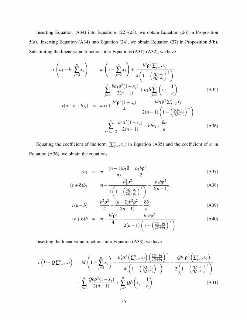
Inserting Equation (A34) into Equations (22)-(23), we obtain Equation (26) in Proposition
5(a). Inserting Equation (A34) into Equation (24), we obtain Equation (27) in Proposition 5(b).
Substituting the linear value functions into Equations (A31)-(A32), we have
r
(a1−b1
n
∑j=2
x j
)= m
(1−
n
∑j=2
x j
)+
b21ρ2
∑nj=2 x j
4(
1−(
2Q−b12Q+b1
)+)
−n
∑j=2
bb1ρ2(1− x j)2(n−1)
+b1δ
n
∑j=2
(x j−
1n
), (A35)
r(a−b+bxi) = mxi +b2ρ2(1− xi)
4−
bb1ρ2∑
nj=2 x j
2(n−1)(
1−(
2Q−b12Q+b1
)+)
−n
∑j 6=i, j=2
b2ρ2(1− x j)2(n−1)
−δbxi +δbn
. (A36)
Equating the coefficient of the term (∑nj=2 x j) in Equation (A35) and the coefficient of xi in
Equation (A36), we obtain the equations
ra1 = m− (n−1)b1δ
n)− b1bρ2
2, (A37)
(r +δ)b1 = m−b2
1ρ2
4(
1−(
2Q−b12Q+b1
)+) − b1bρ2
2(n−1), (A38)
r(a−b) =b2ρ2
4− (n−2)b2ρ2
2(n−1)+
δbn
, (A39)
(r +δ)b = m− b2ρ2
4− b1bρ2
2(n−1)(
1−(
2Q−b12Q+b1
)+) . (A40)
Inserting the linear value functions into Equation (A33), we have
r(
P−Q∑nj=2 x j
)= M
(1−
n
∑j=2
x j
)−
b21ρ2(
∑nj=2 x j
)(2Q−b12Q+b1
)+
4((
1−(
2Q−b12Q+b1
)+) +
Qb1ρ2(
∑nj=2 x j
)2(
1−(
2Q−b12Q+b1
)+)
−n
∑j=2
Qbρ2(1− x j)2(n−1)
+n
∑j=2
Qδ
(x j−
1n
). (A41)
35

Equating the coefficients of the term (∑nj=2 x j) in Equation (A41), we obtain
rP = M− (n−1)Qδ
n− Qbρ2
2, (A42)
(r +δ)Q = M +b2
1ρ2(
2Q−b12Q+b1
)+
4(
1−(
2Q−b12Q+b1
)+)2 −
Qb1ρ2
2(
1−(
2Q−b12Q+b1
)+) − Qbρ2
2(n−1). � (A43)
Proof of Corollary 2
Setting θ∗ = 0, a1 = a, and b1 = b in Equations (A40)-(A43) and solving for a, b, P, and Q, we
obtain Equation (29) and Equation (31) in Corollary 2. �
Proof of Proposition 6
Since b > 0 and Q > 0, the sign of(
2Q−b2Q+b
)is the same as the sign of 2Q/b−1. Therefore, we set
the threshold S = 2Q/b−1. �
Proof of Corollary 3
This result can be obtained by setting r = δ = 0 in Proposition 6. �
APPENDIX B
Selling Through All Retailers
Up to this point, we have assumed that only one retailer is supported by the manufacturer. This
might be the case if a manufacturer sells to retailers whose locations are dispersed. Suppose now
that the manufacturer sells through all retailers. A noteworthy case arises when the manufacturer’s
margin is equal across all n retailers. Obviously, if this common margin is M, then the manufacturer
captures the whole market at this margin regardless of the individual market shares of the retailers
36

and their parameters. It is then clear that the manufacturer has no need to support any of the
retailers θ∗i = 0, i = 1,2, ...,n. Then, clearly the value function of the manufacturer is
∫∞
0e−rt(Mx(t)+M(1− x(t)))dt =
∫∞
0e−rtMdt = M/r.
It is possible that there are other parameter combinations for which θ∗i = 0, i = 1,2, ...,n, which
need to be derived to allow us to understand those situations where a manufacturer does not provide
any advertising support to its retailers. For the cases where θ∗i = 0, i = 1,2, ...,n, we can see that
the manufacturer’s and the retailers’ problems are decoupled. Having solved the manufacturer’s
problem, we see that the retailers’ problem is reduced to the Nash differential game that was solved
in Prasad and Sethi (2004).
Next, we take up the case when the manufacturer’s margins are not equal across all retailers.
Here, we limit our analysis to the situation where retailers are symmetric, as before, but Mi > 0,
i = 2,3, ...,n. Instead we assume that the manufacturer sells to Retailer 1 at a margin M and to the
other symmetric retailers at a common margin Mi = µ > 0, i ∈ {2,3, ...,n}. The manufacturer sets
the participation rates for Retailer i at θi(x2,x3, ...,xn) and then retailers choose advertising efforts
ui. Thus, Retailer i maximizes
Vi = maxui(t), t≥0
∫∞
0e−rt (mxi− (1−θi(x2(t),x3(t), ...,xn(t)))u2
i (t))
dt, i = 1,2, ...n.(A44)
Solving the Nash differential game with the objective functions in Equation (A44) yields Re-
tailer i’s feedback advertising effort, denoted ui(x2,x3, ...,xn|θ1,θ2, ...,θn). The manufacturer an-
ticipates the retailers’ reaction functions when solving for its subsidy rates. Therefore, the manu-
facturer’s problem is given by
V = maxθ1(t), θ2(t),..., θn(t) t≥0
∫∞
0e−rt
(Mx(t)+µ(1− x(t))−
n
∑i=1
θi(t)u2i (t)
)dt (A45)
37

subject to the retail dynamics.
For the Stackelberg-Nash game defined by Equations (A44), (A45), and (18), we have the
following result.
Proposition 7: For symmetric retailers, it is never optimal for the manufacturer to support all
retailers. In particular, when M > µ ≥ 0, only the first retailer may be supported (θ∗1 ≥ 0) and
θ∗i = 0, i ∈ {2,3, ...,n}.
Proof of Proposition 7
First, note that if M > µ, the manufacturer’s objective function in equation (A45) can be organized
as follows:
∫∞
0e−rt
(µ+(M−µ)x−θ1u2
1 (x)−n
∑j=2
θ ju2j (x)
)dt.
This means that the manufacturer should encourage Retailer 1 to increase advertising in order
to increase market share (and discourage the other retailers from advertising by setting θ∗j = 0,
j ∈ {2,3, ...,n}). �
To summarize, we have treated two special cases of selling through all retailers in this section.
If manufacturer’s margins are equal across retailers, no one gets a subsidy. If the manufacturer
has a higher margin from Retailer 1 than it has from all other retailers, which are assumed to be
symmetric and to be providing equal margins to the manufacturer, then the only retailer that might
be supported is Retailer 1. The case with asymmetric retailers is rather intractable, although some
other special cases may be solvable.
Retail Price Competition
We present an extension of the model specified by Equations (1)-(5) that includes retail (but not
wholesale) price competition to show the robustness of the results to the inclusion of price. We let
38

the retailers choose their prices after deciding their advertising levels. The optimal prices resulting
from this formulation are then substituted to yield the retailers margins. This is similar to the Bass
et al. (2005) approach. Thus, the model with endogenous retail price competition reduces to the
current model with exogenous margins.
Retailer i’s discounted profit maximization problem, i = 1,2, is given by
Vi(x0) = maxui(t), pi(t)
∫∞
0e−rt (Di(pi (t) , p3−i (t))(pi (t)− ci)xi (t)− (1−θi(x(t)))u2
i (t))
dt, (A46)
subject to Equation (1), where pi (t) is the price charged by Retailer i,
Di(pi (t) , p3−i (t)) = (1−hi pi (t)+d3−i p3−i (t))
is the demand function expressed as a function of the prices of the two retailers, ci is the marginal
cost of Retailer i, and hi and di are demand parameters. Solving for the retailers’ optimal prices
yields
pi =d3−i +h3−i (2+2hici +d3−ic3−i)
4h1h2−d1d2, i = 1,2. (A47)
Using the parameter mi to denote (Di(pi (t) , p3−i (t)))(pi (t)− ci) in Equation (A46), where pi = pi
from Equation (A47), results in Equations (2)-(3). The demand parameters affect price, which
in turn affects the profit margins. Thus, the results in the Analysis and Results section remain
unchanged except that we can now add that the demand parameters affect the subsidy rate θ∗ via
mi, i ∈ {1,2}.
39

Table A1: Notation.
t Time t, t ≥ 0
x(t) ∈ [0,1] Retailer 1’s share of the market at time t
x0 Initial market share of Retailer 1
ui (t)≥ 0 Retailer i’s advertising effort rate at time t, i = 1,2
θ(t)≥ 0 Manufacturer’s subsidy rate for Retailer 1 at time t
ρi > 0 Advertising effectiveness parameter
δi ≥ 0 Market share decay parameter
r > 0 Discount rate of the retailers and the manufacturer
mi > 0 Gross margin of Retailer i
M ≥ 0 Gross margin of the manufacturer from Retailer 1
Vi, V Value functions of Retailer i and the manufacturer, respectively
f ′(x) or f ′ d f /dx for a differentiable function f (x)
f (x)+ or f + max{ f (x),0} for a function f (x)
Figure 1: Market structure.
40

Figure 2: Effect of retailers’ margins on the optimal subsidy rate.
Figure 3: Effect of advertising effectiveness on the optimal subsidy rate.
41

Figure 4: Effect of decay rate on the optimal subsidy rate.
Figure 5: Effect of competition on the optimal subsidy rate.
42