Co-domain Embedding using Deep Quadruplet Networksfor Unseen Traffic Sign Recognition

Junsik Kim Seokju Lee Tae-Hyun Oh† In So KweonDept. of Electrical Engineering, KAIST, Daejeon, Korea

†MIT CSAIL, Cambridge, USmibastro,seokju91@gmail.com, taehyun@csail.mit.edu†, iskweon@kaist.ac.kr

Abstract

Recent advances in visual recognition show overarching suc-cess by virtue of large amounts of supervised data. However,the acquisition of a large supervised dataset is often challeng-ing. This is also true for intelligent transportation applications,i.e., traffic sign recognition. For example, a model trainedwith data of one country may not be easily generalized to an-other country without much data. We propose a novel featureembedding scheme for unseen class classification when therepresentative class template is given. Traffic signs, unlikeother objects, have official images. We perform co-domain em-bedding using a quadruple relationship from real and syntheticdomains. Our quadruplet network fully utilizes the explicitpairwise similarity relationships among samples from differ-ent domains. We validate our method on three datasets withtwo experiments involving one-shot classification and featuregeneralization. The results show that the proposed methodoutperforms competing approaches on both seen and unseenclasses.

IntroductionRecent advances in the field of computer vision have providedhighly cost-effective solutions for developing advanced driverassistance systems (ADAS) for automobiles. Furthermore,computer vision components are becoming indispensableto improve safety and to achieve AI in the form of fullyautomated, self-driving cars. This is mostly by virtue of thesuccess of deep learning, which is regarded to be due to thepresence of large-scale supervised data, proper computationpower and algorithmic advances (Goodfellow, Bengio, andCourville 2016).

Among all ADAS related problems, in this paper, we tackleunseen traffic sign recognition. A distinctive difference re-lated to this problem as regards traditional recognition prob-lems is that synthetic traffic-sign templates are exploited asrepresentative anchors, whereby classification can be donefor an actual query image by finding the minimum distanceto the templates of each class (i.e., few-shot learning withdomain difference).

In reality, traffic signs differ depending on the country,but one may obtain synthetic templates from traffic-relatedpublic agencies. Nonetheless, the diversity of templates for a

Copyright c© 2018, Association for the Advancement of ArtificialIntelligence (www.aaai.org). All rights reserved.

single class is limited; hence, we focus on scenarios of chal-lenging one-shot classification (Koch, Zemel, and Salakhut-dinov 2015; Lake, Salakhutdinov, and Tenenbaum 2015;Miller, Matsakis, and Viola 2000) with domain adaptation,where a machine learning model must generalize to newclasses not seen in the training phase given only a few exam-ples of each of these classes but from different domains.

In practice, this type of model is especially useful forADAS in that: 1) one can avoid high cost re-training fromscratch, 2) one can avoid annotating large-scale superviseddata, and 3) it is readily possible to adapt the model to otherenvironments.

Given the success of deep learning, a naive approach forthe few-shot problem would be to re-train a deep learningmodel on a new scarce dataset. However, in this limiteddata regime, this type of naive method will not work well,likely due to severe over-fitting (Lake, Salakhutdinov, andTenenbaum 2015). While people have an inherent ability togeneralize from only a single example with a high degree ofaccuracy, the problem is quite difficult for machine learningmodels (Lake, Salakhutdinov, and Tenenbaum 2015).

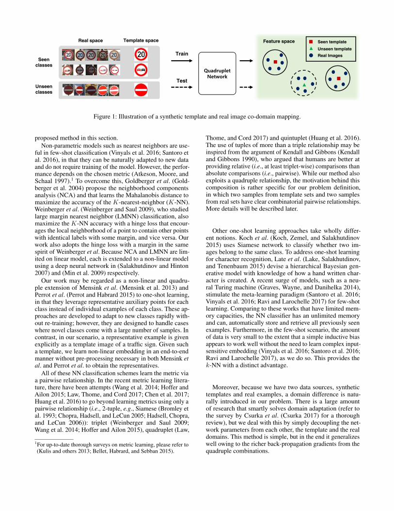
Thus, our approach is based on the following hypothe-ses: 1) the existence of a co-embedding space for syntheticand real data, and 2) the existence of an embedding spacewhere real data is condensed around a synthetic anchor foreach class. We illustrate the idea in Fig. 1. Taking these intoaccount, we learn two non-linear mappings using a neuralnetwork. The first involves mapping for a real sample intoan embedding space, and the second involves mapping of asynthetic anchor onto the same metric space. We leverage thequadruplet relationship to learn non-linear mappings, whichcan provide rich information to learn generalized and dis-criminative embeddings. Classification is then performed foran embedded query point by simply finding the nearest classanchor. Despite its simplicity, our method outperforms witha margin in the unseen data regime.

Related workOur problem can be summarized as a modified one-shot learn-ing problem that involves heterogeneous domain datasets.This type of problem has gained little attention. Furthermore,to the best of our knowledge, our work is the first to tackleunseen traffic sign recognition with heterogeneous domaindata; we therefore summarize the work most relevant to our

arX

iv:1

712.

0190

7v1

[cs

.CV

] 5

Dec

201

7

Real space Template space

Seenclasses

Unseenclasses

Train

Test

Feature space Seen template

Unseen template

Real Images

Embedding model

Real space Template space

Seenclasses

Unseenclasses

Train

Test

Feature space Seen template

Unseen template

Real Images

QuadrupletNetwork

Figure 1: Illustration of a synthetic template and real image co-domain mapping.

proposed method in this section.Non-parametric models such as nearest neighbors are use-

ful in few-shot classification (Vinyals et al. 2016; Santoro etal. 2016), in that they can be naturally adapted to new dataand do not require training of the model. However, the perfor-mance depends on the chosen metric (Atkeson, Moore, andSchaal 1997).1 To overcome this, Goldberger et al. (Gold-berger et al. 2004) propose the neighborhood componentsanalysis (NCA) and that learns the Mahalanobis distance tomaximize the accuracy of the K-nearest-neighbor (K-NN).Weinberger et al. (Weinberger and Saul 2009), who studiedlarge margin nearest neighbor (LMNN) classification, alsomaximize the K-NN accuracy with a hinge loss that encour-ages the local neighborhood of a point to contain other pointswith identical labels with some margin, and vice versa. Ourwork also adopts the hinge loss with a margin in the samespirit of Weinberger et al. Because NCA and LMNN are lim-ited on linear model, each is extended to a non-linear modelusing a deep neural network in (Salakhutdinov and Hinton2007) and (Min et al. 2009) respectively.

Our work may be regarded as a non-linear and quadru-ple extension of Mensink et al. (Mensink et al. 2013) andPerrot et al. (Perrot and Habrard 2015) to one-shot learning,in that they leverage representative auxiliary points for eachclass instead of individual examples of each class. These ap-proaches are developed to adapt to new classes rapidly with-out re-training; however, they are designed to handle caseswhere novel classes come with a large number of samples. Incontrast, in our scenario, a representative example is givenexplicitly as a template image of a traffic sign. Given sucha template, we learn non-linear embedding in an end-to-endmanner without pre-processing necessary in both Mensink etal. and Perrot et al. to obtain the representatives.

All of these NN classification schemes learn the metric viaa pairwise relationship. In the recent metric learning litera-ture, there have been attempts (Wang et al. 2014; Hoffer andAilon 2015; Law, Thome, and Cord 2017; Chen et al. 2017;Huang et al. 2016) to go beyond learning metrics using only apairwise relationship (i.e., 2-tuple, e.g., Siamese (Bromley etal. 1993; Chopra, Hadsell, and LeCun 2005; Hadsell, Chopra,and LeCun 2006)): triplet (Weinberger and Saul 2009;Wang et al. 2014; Hoffer and Ailon 2015), quadruplet (Law,

1For up-to-date thorough surveys on metric learning, please refer to(Kulis and others 2013; Bellet, Habrard, and Sebban 2015).

Thome, and Cord 2017) and quintuplet (Huang et al. 2016).The use of tuples of more than a triple relationship may beinspired from the argument of Kendall and Gibbons (Kendalland Gibbons 1990), who argued that humans are better atproviding relative (i.e., at least triplet-wise) comparisons thanabsolute comparisons (i.e., pairwise). While our method alsoexploits a quadruple relationship, the motivation behind thiscomposition is rather specific for our problem definition,in which two samples from template sets and two samplesfrom real sets have clear combinatorial pairwise relationships.More details will be described later.

Other one-shot learning approaches take wholly differ-ent notions. Koch et al. (Koch, Zemel, and Salakhutdinov2015) uses Siamese network to classify whether two im-ages belong to the same class. To address one-shot learningfor character recognition, Late et al. (Lake, Salakhutdinov,and Tenenbaum 2015) devise a hierarchical Bayesian gen-erative model with knowledge of how a hand written char-acter is created. A recent surge of models, such as a neu-ral Turing machine (Graves, Wayne, and Danihelka 2014),stimulate the meta-learning paradigm (Santoro et al. 2016;Vinyals et al. 2016; Ravi and Larochelle 2017) for few-shotlearning. Comparing to these works that have limited mem-ory capacities, the NN classifier has an unlimited memoryand can, automatically store and retrieve all previously seenexamples. Furthermore, in the few-shot scenario, the amountof data is very small to the extent that a simple inductive biasappears to work well without the need to learn complex input-sensitive embedding (Vinyals et al. 2016; Santoro et al. 2016;Ravi and Larochelle 2017), as we do so. This provides thek-NN with a distinct advantage.

Moreover, because we have two data sources, synthetictemplates and real examples, a domain difference is natu-rally introduced in our problem. There is a large amountof research that smartly solves domain adaptation (refer tothe survey by Csurka et al. (Csurka 2017) for a thoroughreview), but we deal with this by simply decoupling the net-work parameters from each other, the template and the realdomains. This method is simple, but in the end it generalizeswell owing to the richer back-propagation gradients from thequadruple combinations.

Quadruple network for jointly adaptingdomain and learning embedding

Our goal is to learn embeddings, such that different domainexamples are embedded into a common metric space andwhere their embedded features favor to be generalized aswell as discriminative.

To this end, we leverage a quadruplet relationship, con-sisting of two anchors of different classes and two othersfor examples corresponding to the anchors. We first describethe quadruple (4-tuple) construction in the following section.Subsequently, we define the embeddings followed by theobjective functions and quadruplet network.Notation We consider two imagery datasets: the templateset T =(T, y), where each T denotes a representative tem-plate image and y∈1, . . . , C is the corresponding label (outof the C class), and the real example set X=XkCk=1, whereXk is the set of real images X of class-k. For simplicity,we use Tk (Xk) to denote a sample labeled with class-k.

We define Euclidean embeddings as f(·), where f(x)maps a high-dimensional vector x into a D-dimensional fea-ture space, i.e., e=f(x) ∈ RD.

Quadruple (4-tuple) constructionOur idea is to embed template and real domain data into thesame feature space such that a template sample acts as ananchor point on the feature space and real samples relevantto the anchor form a cluster around it, as illustrated in Fig. 1.Specifically, we aim to achieve two properties for an em-bedded feature space: 1) distinctiveness between anchors isfavored, and 2) real samples must be mapped close to theanchor that corresponds to the same class.

To leverage the relational information, we define a quadru-ple, a basic element, by packing two template images fromdifferent classes and two real images corresponding to respec-tive template classes, i.e., for simplicity, two classes A andB are considered, then (TA,TB ,XA,XB). From pairwisecombinations within the quadruple, we can reveal severaltypes of relational information as follows:1© TA should be far from TB in an embedding space,2©XA should be far from XB in an embedding space,3©XA (or XB) should be close to TA (or TB) in an embed-

ding space,4©TA (or TB) should be far from XB (or XA) in an embed-

ding space,whereby we derive the final objective function. These rela-tions depicted in Fig. 2b.

Quadruple sampling We sampled two templates (TA, y)and (TB , y

′) from template set T while guaranteeing twodifferent classes, followed by the two real images of XA ∈Xy and XB ∈ Xy′ .

Comparison to other tuple approaches In metriclearning, the most common approaches would be theSiamese (Bromley et al. 1993; Chopra, Hadsell, and LeCun2005; Hadsell, Chopra, and LeCun 2006) and triplet (Wein-berger and Saul 2009; Wang et al. 2014; Hoffer and Ailon

2015), which typically use 2- and 3-tuples, respectively. Fromthe given tuple, they optimize with the pairwise differences.This concept can be viewed as follows: given a tuple, theSiamese has only a single source of loss (and its gradient),while triplets utilize two sources, i.e., (query, positive) and(query, negative). With this type of simple comparison, wecan intuitively conjecture higher stability or performance oftriplet network over Siamese network.

Law et al. (Law, Thome, and Cord 2017) deal with a par-ticular ambiguous quadruple relationship (a)≺(b)'(c)≺(d)by forcing the difference between (b) and (c) to be smallerthan the difference between (a) and (d). Huang et al. (Huanget al. 2016) (quintuplet, 5-tuple) is devised a means to handleclass imbalance issues by leveraging the relationships amongthree levels (e.g., strong, weaker and weakest in terms of acluster analysis) of positives and negatives. Comparing themotivations of these approaches, for instance indefinite rela-tiveness, our quadruple comes from a specific relationship,i.e., heterogeneous domain data. Moreover, it is important tonote that our quadruple provides richer information (a totalof 6 pairwise information) compared to the method of Law etal. (quadruplet) which leverages a single constraint from aquadruple. It is even richer than Huang et al. (quintuplet),who provides 3 constraints.

Quadruplet NetworkGiven the defined quadruple, we propose a quadruple met-ric learning that learns to embed template images and realimages into a common metric space, say RD, through anembedding function. In order to deal with non-linear map-ping, the embedding f is modeled as a neural network, ofwhich set of weight parameters are denoted as θ. Since wedeal with data from two different domains, template and realimages, we simply use two different neural networks θT andθR for the template and real images respectively, expressed asfT(·)=f(· ;θT) and fR(·)=f(· ;θR), such that we can adaptboth domains. Now, we are ready to define the proposedquadruple network.

The proposed quadruple network Q is composed of twoSiamese networks, the weights of which are shared withineach pair. One part embeds features from template imagesand the other part for real images. Quadruple images fromeach domain are fed into the corresponding Siamese networks(depicted in Fig. 2a), and denoted as

Q(

(TA,TB ,XA,XB) ;θT,θR

)=

[fT(TA), fT(TB), fR(XA), fR(XB)

]=

[eAT , e

BT , e

AX , e

BX

],

(1)

for two different arbitrary classes A and B, where e∈Rd

represents the embedded vector mapped by the embeddingfunction f .

Loss function We mainly utilize the l2 hinge embed-ding loss with a margin to train the proposed network.Given outputs quadruplet features

[eAT , e

BT , e

AR , e

BR

], we

have up to six pairwise relationships, as shown in Fig. 2b),and obtain six pairwise Euclidean feature distances as

Template domain tower

Real domain tower

;

;

;

;

Embedded vectorInput Base network

(a)

Template domain tower

Real domain tower

;

;

;

;

Embedded vectorInput Base network

(b)

Figure 2: (a) Quadruplet network structure. (b) pairwise rela-tions of embedded vectors.

d(ekj , ek′

j′ )k,k′∈A,B

j,j′∈T,R , where d(a, b) = ‖a−b‖2 denotesthe Euclidean distance. Let hm(d) denote the hinge loss withmargin m as hm(d) = max(0,m−d), where d is the dis-tance value. We then encourage the embedded vectors withthe same label pairs (i.e., if k = k′) to be close by applyingthe loss h−m(−d), while pushing away the different labelpairs by applying hm′(d).

To induce the embedded feature space with the aforemen-tioned two properties in the Quadruple Construction section,the minimum number of necessary losses is three, while wecan exploit up to six losses; hence, we have several choicesto formulate the final loss function, as described below:

HingeM-3 : L3m,m′= hm

(d(eAT , e

BT

))+h−m′

(d(eAT , e

AX

))+ h−m′

(d(eBT , e

BX

)), (2)

HingeM-5 : L5m,m′= L3m,m′ + hm

(d(eAT , e

BX

))+hm

(d(eAX , e

BT

)), (3)

HingeM-6 : L6m,m′= L5m,m′ + hm

(d(eAX , e

BX

)). (4)

In addition, inspired by the contrastive loss (Chopra, Had-sell, and LeCun 2005), we also adopt an alternative loss by re-placing the h−m(−d) terms in Eq. (2) with directly minimiz-ing d.2 We denote this alternative loss simply as contrastivewith a slight abuse of the terminology. We will compare these

2This can be viewed as a l1 version of the contrastiveloss (Chopra, Hadsell, and LeCun 2005); this is howHingeEmbeddingCriterion is implemented for the pairwiseloss in Torch7 (Collobert, Kavukcuoglu, and Farabet 2011).

losses in the Experiments section. Analogous to traditionaldeep metric learning, training with these losses can be donewith a simple SGD based method. By using shared parameternetworks, the back-propagation algorithm updates the mod-els w.r.t. several relationships; e.g., in the HingeM-6 case,the template tower is updated w.r.t. 5 pairwise relationships(i.e., (TA,TB), (TA,XA), (TB ,XB), (TA,XB), (XA,TB)),analogously for the real tower.

ExperimentsExperiment setupCompeting methods We compare the proposed methodwith other deep neural network based previous works and theadditionally devised baseline, as follows:

- IdsiaNet (CiresAn et al. 2012) is a competition winner ofthe German Traffic-Sign Recognition Benchmark (Stal-lkamp et al. 2012) (GTSRB). We directly used an im-proved implementation (The Moodstocks team repository).3 For all of the experiments, IdsiaNet is exhaustivelycompared as a supervised model baseline, in the same phi-losophy of the deep generic feature (Donahue et al. 2014).Moreover, templates are not used for training. For a faircomparison, the architecture itself is adopted as the basenetwork for the following models.

- Triplet (Hoffer and Ailon 2015) (Hoffer et al.) is similarto our model but with triplet data. Three weight sharednetworks are used, while in training, we randomly sampledtriplets within the real image set with labels, such that notemplate image is exposed during triplet training. Thistraining method is consistent with Hoffer et al.

- Triplet-DA (domain adaptation) is a variant devised byus to test our hypothesis that involving different domaintemplates as an anchor is beneficial. Three weight sharednetworks are used, and for triplet sampling, we sampleone template (T, y) from template set T and then sam-ple positive and negative real images from Xy and Xk 6=y

respectively.

Implementation details For fairness, all of the details areequally applied unless otherwise specified. All input imagesare resized to 48×48 and the mean intensity of training setis subtracted. We did not perform any further preprocessing,data augmentation, or ensemble approach.

We use the same improved IdsiaNet (The Moodstocks teamrepository ) for the base network of Triplet, Triplet-DA andour Quadruplet, but replace the output dimension of the finallayer FC2 to be RD without a softmax layer. Every model istrained from scratch. Most of the hyper parameters are basedon the implementation (The Moodstocks team repository )with a slight modification (i.e., fixed learning rates: 10−3,momentum: 0.9, weight decay: 10−4, mini-batch size: 100,

3The improved performance is reported in (The Moodstocks teamrepository ) with an even simpler architecture and without usingensemble. For brevity, we denote this improved version simply asIdsiaNet. Detailed information can also be found in the supplemen-tary material.

optimizer: stochastic gradient descent). Models are traineduntil convergence is reached, i.e., Lt−Lt−1

Lt−1<5% where Lt

denotes the loss value at t-th iteration. We observed thatthe models typically converged at around 15k-20k iterations.All networks were implemented using Torch7 (Collobert,Kavukcuoglu, and Farabet 2011).

DatasetWe use two traffic-sign datasets, GTSRB (Stallkamp etal. 2012) and Tsinghua-Tencent 100K (Zhu et al. 2016)(TT100K). Since our motivation can be considered to involvedealing with a deficient data regime and a data imbalancecaused by rare classes, we additionally introduce a subsetsplit from GTSRB, referred to here as GTSRB-sub. To utilizethe dataset properly for our evaluation schemes, given thetrain and test set splits provided by the authors, we furthersplit them into seen, unseen and validation partitions, as illus-trated in Fig. 3. The validation set is constructed by randomsampling from the given training set. A description of thedataset construction process follows. For more details, thereader can refer to the supplementary material.

Ω𝑠Ψ𝑠Φ𝑠

Train Val. Test

Seen

Unseen

Ψ𝑢Φ𝑢 Ω𝑢

Figure 3: Partitions of dataset.

GTSRB-all GTSRBcontains 43 classes. Thedataset contains severeillumination variation,blur, partial shadingsand low-resolutionimages. The benchmarkprovides partitions intotraining and test sets.The training set contains 39k images, where 30 consecutivelycaptured images are grouped, called a “track”. The test setcontains 12k images without continuity and, thus does notform tracks. We selected 21 classes that have the fewestsamples as unseen classes with the remaining 22 classes asthe seen classes. Template images are involved in the dataset.GTSRB-sub To analyze the performance of the deficientdata regime, we created a subset of GTSRB-all, forming asmaller but class-balanced training set with sharing the testset of GTSRB-all. Hence, numeric results will be compatiblycomparable to that from GTSRB-all. For the training set,we randomly select 7 tracks (i.e., 210 images) for each seenclasses.TT100K-c The TT100K detection dataset includes over200 sign classes. We cropped traffic sign instances from thescenes to build the classification dataset (called TT100K-c). Although it contains the huge number of classes, mostof the classes do not have enough instances to conduct theexperiment. We only selected classes having official tem-plates4 available and a sufficient number of instances. Wesplit TT100K-c into the train and test set according to thenumber of instances. We set 24 classes with ≥100 instancesfor seen classes and select 12 unseen classes as those having50-100 instances. The training set includes half of the seenclass samples, and the other half is sorted into the test set.

4The official templates are provided by the Beijing Traffic Manage-ment Bureau at, http://www.bjjtgl.gov.cn/english/trafficsigns/index.html.

Table 1: Evaluations of the proposed quadruplet network withvarying parameters. Evaluation is conducted on the validationset of GTSRB-all. Accuracy (%) on validation set is reported.

Embedding dim( HingeM-5 )

Top1 NN

Avg. Seen Unseen

D = 50 67.1 92.2 40.8D = 100 69.1 95.3 41.6D = 150 68.9 94.2 42.4

(a) Varying embedding dimension d.

Loss terms(dim 100)

Top1 NN

Avg. Seen Unseen

HingeM-3 67.3 93.1 40.3HingeM-5 69.1 95.3 41.6HingeM-6 68.9 97.3 39.2

(b) Varying number of pairwise loss terms.

Figure 4: Some of failure cases for unseen recognition.

One-shot classificationWe perform one-shot classification by 1-nearest neighbor(1-NN) classification. For 1-NN, the Euclidean distance ismeasured between embedding vectors by forward-feedinga query (real image) and the anchors (template images) tothe network, after which the most similar anchor out of theC classes is found (C-way classification). For the NN per-formance, we measure the average accuracy for each class.The seen class performance is also reported for a referencepurpose.

Self-Evaluation The proposed Quadruplet network hastwo main factors: the embedding dimension D and the num-ber of pairwise loss terms. We evaluate these on the validationsets Ψs and Ψu of GTSRB-all. The Quadruplet network istrained only with the seen training set Φs.

Embedding dimension: We conduct the evaluation whilevarying the embedding dimension D, as reported in Table 1a.We vary D from 50 to 150 and measure the one-shot classi-fication accuracy. We observed that the overall average ac-curacy across the seen and unseen classes peaked at D=100.While the unseen performance may increase further beyondD = 150, since this sacrifices the seen performance, weselect the dimension with the best average accuracy, i.e.,D = 100, as the reference henceforth.

pairwise loss terms: The quadruplet model gives 6 pos-sible pairwise distances between outputs. Intuitively, three

Table 2: One-shot classification (Top 1-NN) accuracy (%) onthe unseen classes. Performance on seen classes are shownas an additional reference.

Network typeDatasets

Anchor GTSRB GTSRB subset TT100K

Seen Unseen Seen Unseen Seen Unseen

IdsiaNet × 74.6 40.2 59.4 34.7 87.7 14.6Triplet Real 62.6 33.9 54.9 23.5 5.9 1.0

Triplet-DA Template 86.0 54.5 60.8 47.6 86.2 67.1

Quad.+contrastive-5 Template 92.4 42.7 69.2 41.8 92.0 67.5Quad.+hingeM Template 90.8 45.2 70.1 47.8 94.9 67.3

Table 3: One-shot classification (Top 1-NN) accuracy (%)from GTSRB-all to TT100K-c.

Network trained on GTSRB Top1 NNsample average

IdsiaNet 36.5Triplet DA 34.1

Quadruple+hingeM 42.3

possible options, i.e., HingeM-3, HingeM-5 and HingeM-6in Eqs. (2-4), satisfy our co-domain embedding property. Theresults in Table 1b show a trade-off between different losses.HingeM-3 performs worse on both seen and unseen classesthan the others, while the other two have a clear trade-off.This implies that HingeM-3 is not producing enough informa-tion (i.e., gradients) to learn a good feature space. HingeM-5outperforms Loss6 on unseen classes but HingeM-6 is betteron seen classes. We suspect that complex pairwise relation-ships among real samples may lead to a feature space whichis overly adapted to seen classes. This trade off can be usedto adjust between improving the seen class performance orregularizing the model for greater flexibility. We report thefollowing results based on HingeM-5 hereafter.

Comparison to other methods We compare the resultshere with those of other methods on the test sets Ωs and Ωu

of three datasets. All networks are trained only with the seentraining and validation set Φs ∪Ψs of respective datasets.

For IdsiaNet, we use the activation of FC1 for feature em-bedding. For the other networks, we use the final embeddingvectors. For the Quadruplet network, we test two cases withcontrastive-5 and HingeM-5.

Table 2 shows the results on the three datasets, whereTriplet has the lowest performance, while Triplet-DA per-forms well. Moreover, our quadruplet network outperformsTriplet-DA in most of cases for both seen and unseen classes.This supports our hypothesis that the template (also a differ-ent domain) anchor based metric learning and the quadrupletrelationship may be helpful for generalization purposes.

To check the embedding capability of each approach fur-ther, we trained each model on GTSRB Φs ∪Ψs and testedon TT100K-c Ωs ∪ Ωu. This experiment qualifies how thenetworks perform on two completely different traffic signdatasets. Table 3 shows the top1-NN performance of eachmodel. Our model performs best tn the transfer scenario,which implies that good feature representation is learned.

In order to demonstrate quantitatively the behavior of the

Quadruplet network, we visualize unseen examples that areoften confused by Quadruplet in Fig. 4. The unseen classes ofexamples that are highly similar to other classes are challeng-ing even for humans; furthermore due to the poor illuminationcondition, motion blur and low resolution.

Learned representation evaluationIn this experiment, we evaluate the generalization behaviorof the proposed quadruple network, which is analyzed bycomparing the representation power of each network overunseen regimes (and seen class cases as a reference). In orderto assess the representation quality of each method purely,we pre-train competing models and our model for Φs ∪Ψs

of each dataset (i.e., only on seen classes), fix the weightsof these models, and use the activations of FC1 (350 dimen-sions) of them as a feature. Given the features extracted byeach model, we measure the representation performance byseparately training the standard multi-class SVM (Chang andLin 2011) with the radial basis kernel such that the perfor-mance heavily relies on feature representation itself. 5

We use identical SVM parameters (nonlinear RBF kernel,C = 100, tol = 0.001) in all experiments. In contrast to FC1trained only on seen data, the SVM model is trained on bothseen and unseen classes with an equal number of instances perclass, and we vary the number of per class training samples:10, 50, 100, and 200. SVM training samples are randomlysampled from the set Φs ∪Ψs ∪ Φu ∪Ψu (Fig. 3), and theentire test set Ωs ∪ Ωu is used for the evaluation. We reportthe average score and confidence interval by repeating theexperiments 100 times for the case of [No. instances/class:10] and 10 times for the cases of [No. instances/class: 50,100, 200]. For each sampling, we fix a random seed and testeach model with the same data for a fair comparison.

With the three datasets, we show the results of the unseenΩu and seen Ωs test cases in Table 4 and 5, respectively. Theunseen and seen class datasets are mutually exclusive; hence,the errors should be compared in each dataset independently,e.g., the numbers in Table 4-(a) are not directly comparablewith those in Table 5-(a). Instead, we can observe the algo-rithmic behavior difference by comparing Table 4 and 5 withrespect to the relative performance.

In the unseen case in Table 4, for all of the results, theproposed Quadruplet variants outperform the other compet-ing methods, supporting the fact that our method generalizeswell in limited sample regimes by virtue of the richer infor-mation from the quadruples. As an addendum, interestingly,Triplet-DA performs better than Triplet only with GTSRB-sub. We postulate that, in terms of feature description withsome amount of strong supervision support, Triplet gener-alizes better than Triplet-DA, due inherently to the numberof possible triplet combinations of Triplet-DA (|T |·|X |2, andgenerally |T ||X |) is much smaller than that of Triplet dueto the use of a template anchor as an element of triplet, whileTriplet improves all the pairwise possibility of real data (i.e.,|X |3). For the quadruplet case, more pairwise relationships

5We follow an evaluation method conducted in (Tran et al. 2015),where the qualities of deep feature representations are evaluated inthe same way.

Table 4: Feature representation quality comparison for un-seen classes. SVM classification errors (%) are reported withthe datasets, GTSRB-all, GTSRB-sub and TT100K-c, andaccording to the number of SVM training instances per class.Notice that, for all the networks, the classes evaluated in thisexperiment are not used for training the networks, i.e., un-seen classes are used only for SVM training. Marked in boldare the best results for each scenario, as well as other resultswith an overlapping confidence interval with 95%.

Network No. instances/class

200 100 50 10

IdsiaNet 6.14 (±0.50) 6.82 (±0.57) 7.82 (±0.64) 11.01 (±0.31)Triplet 7.22 (±0.33) 7.94 (±0.33) 8.79 (±0.40) 15.83 (±0.38)

Triplet-DA 9.04 (±0.30) 9.35 (±0.42) 10.26 (±0.63) 15.17 (±0.29)

Quad.+cont. 5.30 (±0.14) 6.09 (±0.39) 6.96 (±0.37) 9.59 (±0.23)Quad.+hingeM 3.77 (±0.29) 3.86 (±0.27) 4.13 (±0.30) 7.69 (±0.28)

(a) GTSRB-all.

Network No. instances/class

200 100 50 10

IdsiaNet 17.89 (±0.41) 18.28 (±0.60) 18.34 (±0.79) 25.84 (±1.52)Triplet 17.39 (±0.67) 18.22 (±0.92) 20.49 (±1.64) 30.53 (±2.47)

Triplet-DA 15.84 (±0.38) 16.77 (±0.73) 18.24 (±0.48) 28.43 (±1.61)

Quad.+cont. 12.12 (±0.33) 11.72 (±0.40) 12.83 (±0.43) 18.83 (±1.35)Quad.+hingeM 13.81 (±0.31) 14.26 (±0.38) 15.59 (±0.52) 24.31 (±0.45)

(b) GTSRB-sub.

Network No. instances/class

20

IdsiaNet (CiresAn et al. 2012) 3.71 (±0.35)Triplet (Hoffer and Ailon 2015) 3.70 (±0.30)

Triplet-DA 5.05 (±0.45)

Quad.+cont. 2.97 (±0.31)Quad.+hingeM 2.87 (±0.24)

(c) TT100k-c.

results in higher number of tuple combinations and leads tobetter generalization, even with the use of templates.

In the seen class case in Table 5, our method and IdsiaNetshow comparable performance outcomes with the best ac-curacy levels, while Triplet and Triplet-DA do not performas well. We found that the proposed Quadruplet performsbetter than the other approaches when the number of train-ing instances is very low, i.e., 10 samples per class. Morespecifically, IdsiaNet performs well in the seen class case,but not in the unseen class case compared to Quadruplet.This indicates that the embedding of IdsiaNet is trapped inseen classes rather than in general traffic sign appearances.On the other hand, the proposed method learns more generalrepresentation in that its performance in both cases is higherthan those of its counterparts. We believe that this is due tothe regularization effect caused by the usage of templates.

ConclusionIn this study, we have proposed a deep quadruplet for one-shot learning and demonstrated its performance on the unseentraffic-sign recognition problem with template signs. Theidea is that by composing a quadruplet with a template and

Table 5: Feature representation quality comparison for seenclasses. SVM classification errors (%) are reported with thedatasets, GTSRB-all, GTSRB-sub and TT100K-c, and ac-cording to the number of SVM training instances per class.Marked in bold are the best results for each scenario, as wellas other results with an overlapping confidence interval with95%.

Network type No. instances/class

200 100 50 10

IdsiaNet 3.70 (±0.09) 4.24 (±0.14) 4.72 (±0.18) 6.52 (±0.10)Triplet 5.00 (±0.08) 5.51 (±0.12) 6.22 (±0.16) 9.11 (±0.15)

Triplet-DA 4.75 (±0.12) 5.30 (±0.10) 6.08 (±0.22) 8.99 (±0.13)

Quad.+cont. 4.49 (±0.09) 4.50 (±0.12) 4.65 (±0.11) 5.61 (±0.13)Quad.+hingeM 4.46 (±0.08) 4.63 (±0.12) 4.81 (±0.15) 5.98 (±0.08)

(a) GTSRB-all.

Network type No. instances/class

200 100 50 10

IdsiaNet 7.55 (±0.25) 8.64 (±0.22) 10.13 (±0.43) 17.19 (±0.23)Triplet 10.88 (±0.25) 12.35 (±0.31) 14.28 (±0.27) 24.50 (±0.30)

Triplet-DA 8.78 (±0.30) 10.44 (±0.2) 12.80 (±0.37) 21.15 (±0.28)

Quad.+cont. 6.04 (±0.16) 6.88 (±0.11) 7.92 (±0.28) 12.51 (±0.21)Quad.+hingeM 6.57 (±0.15) 7.54 (±0.23) 8.87 (±0.31) 14.02 (±0.20)

(b) GTSRB-sub.

Network type No. instances/class

20

IdsiaNet (CiresAn et al. 2012) 4.23 (±0.22)Triplet (Hoffer and Ailon 2015) 5.30 (±0.14)

Triplet-DA (100) 5.53 (±0.17)

Quad.+cont. 5.39 (±0.23)Quad.+hingeM 4.33 (±0.14)

(c) TT100k-c.

real examples, the combinatorial relationships enable notonly domain adaptation via co-embedding learning, but alsogeneralization to the unseen regime. Because the proposedmodel is very simple, it can be extended to other domainapplications, where any representative anchor can be given.We think that N > 4-tuple generalization is interesting asa future direction in that there must be a trade-off betweenover-fitting and memory capacities.

AcknowledgmentThis work was supported by DMC R&D Center of SamsungElectronics Co.

References[Atkeson, Moore, and Schaal 1997] Atkeson, C. G.; Moore,A. W.; and Schaal, S. 1997. Locally weighted learning.Artificial Intelligence Review 11(1-5):11–73.

[Bellet, Habrard, and Sebban 2015] Bellet, A.; Habrard, A.;and Sebban, M. 2015. Metric learning. Synthesis Lectureson Artificial Intelligence and Machine Learning 9(1):1–151.

[Bromley et al. 1993] Bromley, J.; Guyon, I.; LeCun, Y.;Sackinger, E.; and Shah, R. 1993. Signature verificationusing a siamese time delay neural network. In NIPS.

[Chang and Lin 2011] Chang, C.-C., and Lin, C.-J. 2011. Lib-svm: a library for support vector machines. ACM Transac-tions on Intelligent Systems and Technology (TIST) 2(3):27.

[Chen et al. 2017] Chen, W.; Chen, X.; Zhang, J.; and Huang,K. 2017. Beyond triplet loss: a deep quadruplet network forperson re-identification. In CVPR.

[Chopra, Hadsell, and LeCun 2005] Chopra, S.; Hadsell, R.;and LeCun, Y. 2005. Learning a similarity metric discrimi-natively, with application to face verification. In CVPR.

[CiresAn et al. 2012] CiresAn, D.; Meier, U.; Masci, J.; andSchmidhuber, J. 2012. Multi-column deep neural networkfor traffic sign classification. Neural Networks 32:333–338.

[Collobert, Kavukcuoglu, and Farabet 2011] Collobert, R.;Kavukcuoglu, K.; and Farabet, C. 2011. Torch7: Amatlab-like environment for machine learning. In NIPSBigLearn Workshop.

[Csurka 2017] Csurka, G. 2017. Domain adaptation in com-puter vision applications. Advances in Computer Vision andPattern Recognition. Springer.

[Donahue et al. 2014] Donahue, J.; Jia, Y.; Vinyals, O.; Hoff-man, J.; Zhang, N.; Tzeng, E.; and Darrell, T. 2014. Decaf:A deep convolutional activation feature for generic visualrecognition. In ICML.

[Goldberger et al. 2004] Goldberger, J.; Roweis, S.; Hinton,G.; and Salakhutdinov, R. 2004. Neighbourhood componentsanalysis. In NIPS.

[Goodfellow, Bengio, and Courville 2016] Goodfellow, I.;Bengio, Y.; and Courville, A. 2016. Deep Learning. MITPress.

[Graves, Wayne, and Danihelka 2014] Graves, A.; Wayne,G.; and Danihelka, I. 2014. Neural turing machines. arXivpreprint arXiv:1410.5401.

[Hadsell, Chopra, and LeCun 2006] Hadsell, R.; Chopra, S.;and LeCun, Y. 2006. Dimensionality reduction by learningan invariant mapping. In CVPR.

[Hoffer and Ailon 2015] Hoffer, E., and Ailon, N. 2015.Deep metric learning using triplet network. In InternationalWorkshop on Similarity-Based Pattern Recognition, 84–92.Springer.

[Huang et al. 2016] Huang, C.; Li, Y.; Change Loy, C.; andTang, X. 2016. Learning deep representation for imbalancedclassification. In CVPR.

[Kendall and Gibbons 1990] Kendall, M., and Gibbons, J. D.1990. Rank Correlation Methods. Oxford Univ.

[Koch, Zemel, and Salakhutdinov 2015] Koch, G.; Zemel,R.; and Salakhutdinov, R. 2015. Siamese neural networksfor one-shot image recognition. In ICML Deep Learningworkshop.

[Kulis and others 2013] Kulis, B., et al. 2013. Metric learn-ing: A survey. Foundations and Trends R© in Machine Learn-ing 5(4):287–364.

[Lake, Salakhutdinov, and Tenenbaum 2015] Lake, B. M.;Salakhutdinov, R.; and Tenenbaum, J. B. 2015. Human-levelconcept learning through probabilistic program induction.Science 350(6266):1332–1338.

[Law, Thome, and Cord 2017] Law, M. T.; Thome, N.; andCord, M. 2017. Learning a distance metric from relativecomparisons between quadruplets of images. InternationalJournal of Computer Vision (IJCV) 121:6594.

[Mensink et al. 2013] Mensink, T.; Verbeek, J.; Perronnin, F.;and Csurka, G. 2013. Distance-based image classification:Generalizing to new classes at near-zero cost. IEEE Transac-tions on Pattern Analysis and Machine Intelligence (PAMI)35(11):2624–2637.

[Miller, Matsakis, and Viola 2000] Miller, E. G.; Matsakis,N. E.; and Viola, P. A. 2000. Learning from one examplethrough shared densities on transforms. In CVPR.

[Min et al. 2009] Min, R.; Stanley, D. A.; Yuan, Z.; Bonner,A.; and Zhang, Z. 2009. A deep non-linear feature mappingfor large-margin knn classification. In ICDM.

[Perrot and Habrard 2015] Perrot, M., and Habrard, A. 2015.Regressive virtual metric learning. In NIPS.

[Ravi and Larochelle 2017] Ravi, S., and Larochelle, H.2017. Optimization as a model for few-shot learning. InICLR.

[Salakhutdinov and Hinton 2007] Salakhutdinov, R., andHinton, G. E. 2007. Learning a nonlinear embedding bypreserving class neighbourhood structure. In AISTATS.

[Santoro et al. 2016] Santoro, A.; Bartunov, S.; Botvinick,M.; Wierstra, D.; and Lillicrap, T. 2016. Meta-learningwith memory-augmented neural networks. In ICML.

[Stallkamp et al. 2012] Stallkamp, J.; Schlipsing, M.; Salmen,J.; and Igel, C. 2012. Man vs. computer: Benchmarking ma-chine learning algorithms for traffic sign recognition. Neuralnetworks 32:323–332.

[The Moodstocks team repository ] The Moodstocks teamrepository. Traffic sign recognition with torch. https://github.com/moodstocks/gtsrb.torch.

[Tran et al. 2015] Tran, D.; Bourdev, L.; Fergus, R.; Torresani,L.; and Paluri, M. 2015. Learning spatiotemporal featureswith 3d convolutional networks. In ICCV.

[Vinyals et al. 2016] Vinyals, O.; Blundell, C.; Lillicrap, T.;Wierstra, D.; et al. 2016. Matching networks for one shotlearning. In NIPS.

[Wang et al. 2014] Wang, J.; Song, Y.; Leung, T.; Rosenberg,C.; Wang, J.; Philbin, J.; Chen, B.; and Wu, Y. 2014. Learningfine-grained image similarity with deep ranking. In CVPR.

[Weinberger and Saul 2009] Weinberger, K. Q., and Saul,L. K. 2009. Distance metric learning for large margin near-est neighbor classification. Journal of Machine LearningResearch 10(Feb):207–244.

[Zhu et al. 2016] Zhu, Z.; Liang, D.; Zhang, S.; Huang, X.; Li,B.; and Hu, S. 2016. Traffic-sign detection and classificationin the wild. In CVPR.

Supplementary MaterialsHere, we present additional details of the baseline networkand datasets that could not be included in the main text dueto space constraints. All figures and references in this supple-mentary file are consistent with the main paper.

Base neural network architectureBase network We select the network based on classifica-tion performance under the assumption that high classifica-tion performance stems from good feature embedding capa-bilities. The Idsia network(CiresAn et al. 2012) is a winnerin a German Traffic Sign Recognition Benchmark (GTSRB)competition. It was reported that variants of the Idsia net-work perform even better. The variant IdsiaNet uses a deeperconvolution kernel size for each layer (Table 6). We use thebest performing Idsia-like network 6 for all three embeddingschemes in the experiments.

Table 6: Variant IdsiaNet structure. Zero pad 2 before eachconv layers. (LCN: local contrast normalization)

Layer Type Size kernel size0 input 48x48x3 -1 conv1 46x46x150 7x72 ReLU 46x46x150 -3 Max pooling 23x23x150 2x24 LCN 23x23x150 7x75 conv2 24x24x200 4x46 ReLU 24x24x200 -7 Max pooling 12x12x200 2x28 LCN 12x12x200 7x79 conv3 13x13x300 4x4

10 ReLU 13x13x300 -11 Max pooling 6x6x300 2x212 LCN 6x6x300 6x613 fc1 350 10800→ 35014 ReLU 350 -15 fc2 43 350→ 4316 softmax 43 -

Details of datasetsGTSRB-all GTSRB (Stallkamp et al. 2012) has been themost widely used and largest dataset for traffic-sign recog-nition. It contains 43 classes categorized into three supercategories: prohibitory, danger and mandatory. The datasetcontains illumination variations, blur, partial shadings andlow-resolution images. The benchmark is partitioned intotraining and test sets. The training set contains 39,209 im-ages, with 30 consecutively captured images grouped, whichis referred to here at a track. The test set contains 12,630images without continuity and thus does not form tracks. Thenumber of samples per class varies, and the sample size alsohas a wide range (Fig. 6 & Fig. 7). To validate the embedding

6IdsiaNet (CiresAn et al. 2012) is tuned to achieve better perfor-mance. Please check the repository, https://github.com/moodstocks/gtsrb.torch#gtsrbtorch

capability of the proposed model, we split the training setinto two sets: seen and unseen (Fig. 5). Our motivation isto overcome the data imbalance caused by rare classes. Weselected 21 classes that have the fewest samples as the unseenclass, using the remaining 22 classes as the seen class. Fortraining, we only used seen classes in the training set.

GTSRB-sub To analyze the performance on a datasetwith a limited size, we created a subset of GTSRB-all, form-ing a smaller size, as a class balanced training set. For thetraining set, we randomly selected seven tracks for each ofthe seen classes. For the test set, we used the same set asused in GTSRB-all; hence results will be compatible withand comparable to those of GTSRB-all.

TT100K-c Tsinghua-Tencent 100K (Zhu et al. 2016)(TT100K) is a chinese traffic sign detection dataset that in-cludes more than 200 sign classes. We cropped traffic signinstances from scenes to build a classification dataset (calledTT100K-c) to validate our model. Although it contains nu-merous classes, most of those in each class do not haveenough instances to allow the experiment to be conducted.We only selected classes with official templates7 availableand a sufficient number of instances. We filtered out instancesthat have side lengths of less than 20 pixels, as they are un-recognizable. We split TT100K-c into the training and testset according to the number of instances. We set 24 classesthat have more than 100 instances as the seen classes, andassign 12 classes with between 50 and 100 instances as theunseen class (Fig. 8). The training set includes half of theseen class samples, with the other half going to the test set.All of the unseen class samples belong to the test set. The sizedistribution and the number of samples per class are providedin Fig. 9 and Fig. 10, respectively.

7The official templates are provided by Beijing Traffic Manage-ment Bureau, http://www.bjjtgl.gov.cn/english/trafficsigns/index.html.

prohibitory

danger

mandatory

other

prohibitory

danger

mandatory

other

Seen classes Unseen classes

Figure 5: GTSRB template images.

0

500

1000

1500

2000

2500

# of

sam

ples

Class id

0

1000

2000

3000

4000

5000

6000

7000

8000

25 30 35 40 45 50 55 60 65 70 75 80 85 90 95 100

105

110

115

120

125

130

135

140

145

~>150

# of

sam

ples

Side length (pixel)

0

200

400

600

800

1000

1200

# of

sam

ples

Class id

0

500

1000

1500

2000

2500

3000

3500

# of

sam

ples

Side length (pixel)

Figure 6: GTSRB class sample distribution. Blue: seenclasses (#22). Orange: unseen classes (#21).

0

500

1000

1500

2000

2500

1 3 5 7 9 11 13 15 17 19 21 23 25 27 29 31 33 35 37 39 41 43

# of

sam

ples

Class id

0

1000

2000

3000

4000

5000

6000

7000

8000

25 30 35 40 45 50 55 60 65 70 75 80 85 90 95 100

105

110

115

120

125

130

135

140

145

~>150

# of

sam

ples

Side length (pixel)

0

200

400

600

800

1000

1200

1 2 3 4 5 6 7 8 9 101112131415161718192021222324252627282930313233343536

# of

sam

ples

Class id

0

500

1000

1500

2000

2500

3000

3500

# of

sam

ples

Side length (pixel)

Figure 7: GTSRB size distribution. Sidelength = (height+width)/2

Seen classes Unseen classes

danger

prohibitory

other

mandatory

danger

prohibitory

other

mandatory

Figure 8: TT100K template images.

0

500

1000

1500

2000

2500

# of

sam

ples

Class id

0

1000

2000

3000

4000

5000

6000

7000

8000

25 30 35 40 45 50 55 60 65 70 75 80 85 90 95 100

105

110

115

120

125

130

135

140

145

~>150

# of

sam

ples

Side length (pixel)

0

200

400

600

800

1000

1200

# of

sam

ples

Class id

0

500

1000

1500

2000

2500

3000

3500

# of

sam

ples

Side length (pixel)

Figure 9: TT100K class sample distribution. Blue: seenclasses (#24). Orange: unseen classes (#12).

0

500

1000

1500

2000

2500

# of

sam

ples

Class id

0

1000

2000

3000

4000

5000

6000

7000

8000

25 30 35 40 45 50 55 60 65 70 75 80 85 90 95 100

105

110

115

120

125

130

135

140

145

~>150

# of

sam

ples

Side length (pixel)

0

200

400

600

800

1000

1200

# of

sam

ples

Class id

0

500

1000

1500

2000

2500

3000

3500

# of

sam

ples

Side length (pixel)

Figure 10: TT100K size distribution. Sidelength =(height + width)/2