Sensors 2011, 11, 5337-5359; doi:10.3390/s110505337

sensors ISSN 1424-8220

www.mdpi.com/journal/sensors

Article

A Novel Cloning Template Designing Method by Using an

Artificial Bee Colony Algorithm for Edge Detection of CNN

Based Imaging Sensors

Selami Parmaksızoğlu * and Mustafa Alçı

Electrical and Electronics Engineering, Engineering Faculty, Erciyes University, Turkey;

E-Mail: malci@erciyes.edu.tr

* Author to whom correspondence should be addressed; E-Mail: selamiparmaksizoglu@gmail.com;

Tel.: +90-352-4374901-32000; Fax: +90-352-4375784.

Received: 1 April 2011; in revised form: 27 April 2011 / Accepted: 13 May 2011 /

Published: 17 May 2011

Abstract: Cellular Neural Networks (CNNs) have been widely used recently in

applications such as edge detection, noise reduction and object detection, which are among

the main computer imaging processes. They can also be realized as hardware based

imaging sensors. The fact that hardware CNN models produce robust and effective results

has attracted the attention of researchers using these structures within image sensors.

Realization of desired CNN behavior such as edge detection can be achieved by correctly

setting a cloning template without changing the structure of the CNN. To achieve different

behaviors effectively, designing a cloning template is one of the most important research

topics in this field. In this study, the edge detecting process that is used as a preliminary

process for segmentation, identification and coding applications is conducted by using

CNN structures. In order to design the cloning template of goal-oriented CNN architecture,

an Artificial Bee Colony (ABC) algorithm which is inspired from the foraging behavior of

honeybees is used and the performance analysis of ABC for this application is examined

with multiple runs. The CNN template generated by the ABC algorithm is tested by using

artificial and real test images. The results are subjectively and quantitatively compared

with well-known classical edge detection methods, and other CNN based edge detector

cloning templates available in the imaging literature. The results show that the proposed

method is more successful than other methods.

OPEN ACCESS

Sensors 2011, 11

5338

Keywords: cellular neural networks; edge detection; artificial bee colony algorithm;

real time imaging sensors

1. Introduction

Chua and Yang introduced the Cellular Neural Network (CNN) model, which enables new

possibilities in signal processing and which can be appropriately implemented as an integrated circuit.

The CNN is formed in a way that the cells are connected in a two-dimensional (2D) network structure,

and it is also able to make simultaneous signal processing [1,2]. In the network structure, a cell is

connected with only the neighboring cells by means of a certain set of parameters. The set of these

parameters determines the dynamic behavior of the CNN and are called “cloning template”. The two

dimensional network architecture of CNNs provides a convenient structure for image processing

applications and real time imaging sensors and, therefore, the major application field of CNNs is image

processing [3,4]. Because of the faster image processing ability of CNN-based imaging sensors and

circuits, complex image processing tasks can also be accomplished successfully. Several complex

image processing applications have been successfully carried out through CNNs [5-11]. For realizing

complex image processing applications based on the CNN structure, preliminary image processing

techniques such as edge detection, diffusion and dilation must be used. Therefore the overall

performance of such task depends strongly on the quality of the preliminary process.

Edge detection is a very important area in the field of computer vision, due to the fact it is used as a

main task or preliminary task for complex image processing techniques such as segmentation,

registration and object recognition and identification. An ideal edge detection process is finalized by an

image which is formed as the set of connected curves of the objects boundaries in an image. The main

indicators demonstrating the quality of edge detection are continuous line detection of the details and

boundaries of the objects, the thinness of the lines and the lack of noise in edge detected image. Edge

detection processes have been widely studied in the literature and several techniques have been

suggested for this purpose. The Canny, Sobel, Prewitt and Robert methods are some of the better-known

edge detection techniques [12]. Each technique used for edge detection has advantages and

disadvantages compared to others when analyzed in terms of the quality indicators of edge detection.

In any case, perfect edge detection on real images is quite difficult because brightness and sharpness in

gray level intensity that distinguishes objects from background in complicated images are not apparent.

Since there are no certain conclusions within the studies introduced in the literature about perfect edge

detection [13], there have been ongoing, extensive studies regarding the edge detection methods that

produce almost perfect results [14,15]. Indeed, the operation principle of CNN is different from the

operation of standard image processing techniques when it is interpreted in term of image processing.

Due to the fact the mask parameter of well-known classical edge techniques is not used in the CNN

structure, the CNN cloning template is designed according to the CNN structure. Design of the cloning

template which determines the dynamic behavior of CNN is an important difficulty because a

generalized template design method does not exist. Various methods have been proposed to determine

such templates. These methods can be classified as analytical methods [16-19], local learning

Sensors 2011, 11

5339

algorithms [20,21] and global learning algorithms [22,23]. The difficulty level of the problem

increases depending on the number of variables and the type of data in all developed methods.

However the solution for such problems using deterministic methods includes difficulties in both the

modeling and solution processes, depending on the structure of the problem. Heuristic methods have

been developed in order to overcome these disadvantages and produce a general solution that does not

depend on the problem structure. The heuristic methods, which are based on population, can reach a

solution fast, due to multiple search procedures [24]. If an appropriate quality metric for use in the

heuristic methods can be defined, the optimal cloning template of CNNs, that must be adjusted

correctly to realize the desired image processing practice, can be designed effectively by using the

heuristic algorithms. Determining the cloning template of CNNs has been dealt with as an important

optimization study and therefore several artificial intelligence based methods (such as Particle Swarm

Optimization (PSO), Genetic Algorithm (GA), Differential Evolution (DE), etc.) have been

proposed [25-33]. However, it is a shortcoming of these studies that results have not been assessed or

compared visually or numerically with known classical techniques and previous studies made in the

CNN area. It is required that the problem to be solved and the artificial intelligent optimization method

should be in conformity and the control parameters of the optimization method should be set

effectively. Since the results obtained with a single run are not sufficient to give a reliable

interpretation of the technique used and the results obtained, determining optimal control parameter

values of the optimization algorithm is possible by examining of results obtained with multiple running

on different control parameter values of optimization. In this way, an idea can be suggested about

whether the optimization technique selected is appropriate for the problem.

The Artificial Bee Colony (ABC) algorithm, inspired by the foraging behavior of honeybees, is a

recently developed optimization algorithm [34]. For several problems, quite successful results have

been obtained by using the ABC algorithm [35]. In addition to the successful results, it has been

observed that the application areas of ABC increase rapidly due to its aspects such as easy

applicability, less dependence on problem type, sensitive research in neighboring space, balancing of

exploration and exploitation properties adaptively, producing effective and robust results regardless

from the initial conditions at any time and fast convergence to the optimal solution when using only a

few control parameters [36-38].

Due to the lack of a robust and effective structure in determining the cloning template, template

designing studies are one of the most attractive research areas in the CNN field and this study aims to

design the edge detecting CNN template through ABC algorithm. To examine the effects of ABC

control parameters, performance analysis is made with multiple runs and the most effective control

parameters for this application are identified by means of the data produced. The design template from

the obtained results of ABC in this study is compared with other heuristic method-based CNN

templates. The results are visually and quantitatively compared with the well-known classical edge

detection methods and the other CNN based edge detectors in the literature by using artificial and

real images.

The organization of the paper is as follows: firstly the CNN structure, cell concept and cloning

template are explained in Section 2. Secondly, in Section 3, the structure of ABC is briefly described.

Section 4 includes the information about how the training image used in the optimization is acquired.

Optimization mechanism used to design cloning template of CNN by means of ABC for this

Sensors 2011, 11

5340

application is presented in this section. Edge detection is made on different images and the results are

compared with those of the widely used edge detection methods and the other CNN based cloning

template in literature. The advantages of the results obtained by means of ABC are determined using

several comparison metrics. Lastly, conclusions and suggestions are provided in Section 5.

2. Cellular Neural Networks (CNNs)

In this section, the structure of CNNs is briefly described. The two-dimensional (2D) network of a

CNN structure is formed by the connection of “cells”. Each cell is connected only to its neighbor cells,

in contrast to artificial neural networks [1-3]. This 2D network structure is also convenient for parallel

processing applications and real time signal processing. With its capability of parallel processing, a

CNN can easily perform image processing applications which pose a heavy load in terms of time and

operation. Differently from a general Central Processor Unit (CPU), the CNN runs in parallel on its

cells. CNN has many advantages over others in term of speed and capability. A general architectural

structure for CNNs is shown in Figure 1.

Figure 1. A general architectural structure of a CNN.

CELL

CELL

CELL

CELL

CELL CELL

CELL

CELL

CELL

CELL CELL

CELL

CELL

CELL

CELL

CELL

CELL

CELL

CELL

CELL CELL

CELL

CELL

CELL

CELL

As shown in Figure 1, each cell in a CNN is directly connected only with the neighbor cells. Due to

the regional inner-cell connections in CNNs, a cell directly affects only its neighbor cells. Cells which

are not directly connected to this cell are indirectly affected while transiting from the initial phase to a

stable phase as a result of the propagation of CNN‟s continuous time dynamics [1]. The cell concept

and the cloning template terms are defined in the following subsections.

2.1. Cell

The cell, which is the basic element of the CNN structure, is composed of structurally linear and

non-linear circuit elements, such as capacitors, linear resistances, linear and non-linear controlled

sources and independent sources. The first CNN cell structure in the literature proposed by Chua [1] is

shown in Figure 2.

Sensors 2011, 11

5341

Figure 2. The circuit of a cell.

Eij

(input)(state) (output)

Iij Cx Rx Ixu(i,j;k,l) RyIxy(i,j;k,l) Iyxij

vyij(t)vxij(t)vuij(t)

In Figure 2, Eij is the independent voltage source, Iij is the independent current source, Cx is the

capacitor, Rx and Ry are linear resistors, Ixu(i,j;k,l) and Ixy(i,j;k,l) are linear voltage controlled current

sources with the characteristics of Ixu(i,j;k,l) = B(i,j;k,l)vukl and Ixy(i,j;k,l) = A(i,j;k,l)vykl, respectively.

i and j indicate inner-cell index and k and l are neighborhood indexes of M × N size network. vxij and Iij

shows the state voltage and bias current values of inner-cell (C(i,j)), respectively. These templates are

described more clearly in Section 2.2. The only nonlinear element is piecewise linear voltage

controlled current source with the characteristics of 1 ( 1 1)2yxij xij xij

y

I v vR

.

In Equation (1), the radius (r) neighborhood of a C(i,j) cell in the CNN is given:

, , |max , , 1 ;1rN i j C k l k i l j r k M l N (1)

When the symmetry property is applied to all CNN, if C(i,j) ∈ Nr(k,l), then C(k,l) ∈ Nr(i,j), for all

C(i,j) and C(k,l) cells. For a CNN, the time dependent (t) situations and output formulas are given in

Equations (2) and (3), respectively:

State Equation:

, , , ,

1, ; , , ; , 1 ;1

r r

xij

xij ykl ukl ij

C k l N i j C k l N i jx

dv tC v t A i j k l v t B i j k l v t I i M j N

dt R

(2)

Output Equation:

1

1 1 , 1 ;12

yij xij xijv t v t v t i M j N (3)

In Equation (2), vukl(t) and vykl(t) are the input voltage and output voltage of the (k,l)th neighbor cell.

vxij(t) and Iij as described above are the state and the bias current values of the cell C(i,j), respectively.

vyij(t) given in Equation (3) is the output voltage equation of piecewise linear function and it is called

the output function. In image processing applications, the input and output voltage of any cell represent

the values of same index number pixel of input image and output image, respectively. The operation

limit of a CNN is between −1 and 1, while any pixel value of an image changes from 1 to 255.

Therefore, pixel values of image are converted into operation limits of the CNN. Eventually, (−1) and

(1) values indicate „black pixel‟ and „white pixel‟, and middle values represent „gray-level pixel‟. In

other words, vuij(t) and vukl(t) indicates values of inner pixel and neighbor pixel in input image while

vyij(t) and vykl(t) indicates value of inner pixel and neighbor pixel in output image, respectively.

Sensors 2011, 11

5342

2.2. CNN Cloning Template

The dynamic behavior of a CNN is determined by the cloning template that can be considered as the

indirect ratio of the inter-cell connections. The feedback cloning template A(i,j;k,l), the feed-forward

cloning template B(i,j;k,l) and threshold cloning template I(i,j) given in Equation (2), form the cloning

template for a cell. The feedback and feed-forward template are related with the outputs and inputs of

neighbor cells. However, the threshold template is only related with the inner-cell. The C(i,j) cell is

connected to neighboring cells at a ratio determined by these cloning template. Realizing the desired

image processing can be done by arranging the values of this cloning template appropriately. For the

r = 1 neighborhood of the cell, the matrix structure of the cloning template A(i,j;k,l), B(i,j;k,l) and I(i,j)

are given in Equation (4).

1, 1 1, 1, 1 1, 1 1, 1, 1

, 1 , , 1 , 1 , , 1

1, 1 1, 1, 1 1, 1 1, 1, 1

, ; , , ; , , ,

i j i j i j i j i j i j

i j i j i j i j i j i j

i j i j i j i j i j i j

a a a b b b

A i j k l a a a B i j k l b b b I i j z i j

a a a b b b

(4)

The statement of Equation (4) can be stated as a general definition as in Equation (5):

1 2 3 1 2 3

4 5 6 4 5 6

7 8 9 7 8 9

a a a b b b

A a a a B b b b I z

a a a b b b

(5)

where A, B and I are represented as the template set, and this set, which is designed for the desired

application, is given in Equation (6) as a vector:

1 2 3 4 5 6 7 8 9 1 2 3, 4 5 6 7 8 9, , , , , , , , , , , , , , , , ,ix a a a a a a a a a b b b b b b b b b z (6)

If the network cloning template of CNN can be arranged according to its purpose, the CNN can

realize the desired simultaneous image processing successfully due to its ability to perform parallel

processing. In the following section, the desired xi template set is obtained by using the ABC

optimization algorithm for realizing edge detection processes on a CNN structure. The optimization

structure and architecture of ABC algorithm are defined the following section.

3. Artificial Bee Colony (ABC) Algorithm

The Artificial Bee Colony (ABC) algorithm is inspired by the foraging behavior of honeybees. The

most prominent properties of an ABC algorithm are easy applicability, less dependence on problem

type, sensitive research, balancing of exploration and exploitation properties adaptively, producing

effective and robust results with using only a few control parameters. In this section, the working

mechanism of the ABC is presented and explained as a new approach to design cloning templates in

this study.

3.1. Basic Principles of ABC Algorithm

This algorithm is developed based on the foraging principle of honeybees. There are three types of

foraging bees in a honey bee colony; employed bees, onlooker bees and the scout bees. At the first

Sensors 2011, 11

5343

stage, half of the colony is composed as employed bees (ne) and the other half is composed as onlooker

bees (no). There is only one employed bee for each nectar source. Nectar sources symbolize possible

solutions. That is, the number of employed bees is equal to the number of nectar sources. The basic

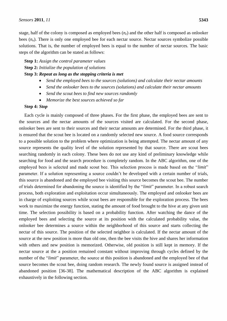
steps of the algorithm can be stated as follows:

Step 1: Assign the control parameter values

Step 2: Initialize the population of solutions

Step 3: Repeat as long as the stopping criteria is met

Send the employed bees to the sources (solutions) and calculate their nectar amounts

Send the onlooker bees to the sources (solutions) and calculate their nectar amounts

Send the scout bees to find new sources randomly

Memorize the best sources achieved so far

Step 4: Stop

Each cycle is mainly composed of three phases. For the first phase, the employed bees are sent to

the sources and the nectar amounts of the sources visited are calculated. For the second phase,

onlooker bees are sent to their sources and their nectar amounts are determined. For the third phase, it

is ensured that the scout bee is located on a randomly selected new source. A food source corresponds

to a possible solution to the problem where optimization is being attempted. The nectar amount of any

source represents the quality level of the solution represented by that source. There are scout bees

searching randomly in each colony. These bees do not use any kind of preliminary knowledge while

searching for food and the search procedure is completely random. In the ABC algorithm, one of the

employed bees is selected and made scout bee. This selection process is made based on the “limit”

parameter. If a solution representing a source couldn‟t be developed with a certain number of trials,

this source is abandoned and the employed bee visiting this source becomes the scout bee. The number

of trials determined for abandoning the source is identified by the “limit” parameter. In a robust search

process, both exploration and exploitation occur simultaneously. The employed and onlooker bees are

in charge of exploiting sources while scout bees are responsible for the exploration process. The bees

work to maximize the energy function, stating the amount of food brought to the hive at any given unit

time. The selection possibility is based on a probability function. After watching the dance of the

employed bees and selecting the source at its position with the calculated probability value, the

onlooker bee determines a source within the neighborhood of this source and starts collecting the

nectar of this source. The position of the selected neighbor is calculated. If the nectar amount of the

source at the new position is more than old one, then the bee visits the hive and shares her information

with others and new position is memorized. Otherwise, old position is still kept in memory. If the

nectar source at the a position remained constant without improving through cycles defined by the

number of the “limit” parameter, the source at this position is abandoned and the employed bee of that

source becomes the scout bee, doing random research. The newly found source is assigned instead of

abandoned position [36-38]. The mathematical description of the ABC algorithm is explained

exhaustively in the following section.

Sensors 2011, 11

5344

3.2. Mathematical Description of ABC Algorithm

In this section, the working mechanism of ABC is presented mathematically. The position of a food

source (xi) represents a feasible solution of problem and the amount of nectar of the food source

indicates the fitness value of the associated solution in the ABC algorithm. The colony size of

employed bees (ne) is equal to the colony size of onlooker bees (no) in the population. A set of food

sources positions (x1,…, xne) is produced randomly:

max0,1min min

i j j jx x rand x x (7)

where i = 1,…,SN and j = 1,..,D. SN is the number of food sources and D is number of optimization

parameters. Also, it must be noted that SN = ne = no. All counters associated with solutions are reset to

0 in this phase. The colony of employed bees can be expressed by ne dimension vector

, where n is cycle value of ABC algorithm. In additional, individual search

space can be signified as S. ∈ and i ≤ ne in . After initialization, the fitness value of each solution

is calculated and is obtained. To evolve quality of solutions, employed bees change their position

from the current position to neighboring source positions by using the following equation:

ij ij ij ij kjv x x x (8)

where ∈ , ∈ , k ≠ j, j and k are randomly chosen index. is a real number

produced randomly in the range [−1,1]. Values of parameters produced in this process are within in

determined boundaries ( ∈ and S → S). After producing vi, to select better solution for next

generation, greedy selection operator is applied. Probability distribution of this operator can be given

as follows:

1,,

0,

i i

i i

i i

f v f xP x v

f v f x

(9)

where f(vi) and f(xi) are nectar amounts of food sources at vi and xi, respectively. If vi is better solution

than xi, the employed bee memorizes position of vi, otherwise position of xi is retained. In the end of

this process, if a better solution cannot be obtained, the trials counter associated with the solution is

incremented by 1, and otherwise it is reset to 0.

After the employed bees phase is completed, the phase of onlooker bees is started by selecting an

employed bee from the colony. The probability of the selection process depends on the fitness values

of the solutions and many selection schemas such as roulette wheel and stochastic universal sampling

can be used. Probabilistic function of roulette wheel mostly used ABC can be described as follows:

1

i

i SN

i

i

f xP x

f x

(10)

This function means that, if the fitness value of a solution increases, the visiting number of onlooker

bees to that source increases too. To decide if a modification will be made on an onlooker bee position,

a random real number within the range [0,1] is generated for each source. If the generated number is

less than the probability value in Equation (10), then the onlooker bee changes position by using

Sensors 2011, 11

5345

Equation (8) to find new solutions. Greedy selection is applied to the modified source and then if the

new position is better than the old position, the memory of the onlooker bee is updated, otherwise the

old position is kept. According to the result of this process, the counter associated with onlooker bees

is incremented by 1 or reset to 0 similar to the operation in the employed bee phase.

To end a cycle, if a counter value of employed bees and onlooker bees reaches its “limit” value, the

source of this counter is abandoned. A new food source is discovered by the scout bee and it replaces

the abandoned source. This operation can be defined as follows:

min max min0,1 ,

1( ),

i

i

x rand x x counter limitx n

x n counter limit

(11)

This operation is a noticeable property of ABC algorithms because this operation is different from

other algorithms and it can improve the search efficiency of the ABC. A detail theoretical explanation

about convergence and complexity analysis of ABC can be found in [39]. ABC optimization study is

explained exhaustively in order to realize proposed application by using ABC in the following section.

4. Proposed Method

It is the aim of this study to effectively determine the edge detection cloning template of the CNN

with an optimization mechanism set up using suitable quality metric and training images. In this

section, the training image used in optimization, the quality metrics and the optimization study

are explained.

4.1. Preparation of Training Images for ABC Optimization

Ideal edge detection of a noise free image which has homogenous objects or regions is achieved by

using the pseudo code given below. The image obtained by using this method is used as the desired

output image of the proposed method in this paper:

start

for i=1:m

for j=1:n

if ePi,j < ePi+1,j then dPi,j=1

if ePi,j < ePi,j+1 then dPi,j=1

if ePi,j > ePi+1,j then dPi+1,j=1

if ePi,j > ePi,j+1 then dPi,j+1=1

end

end

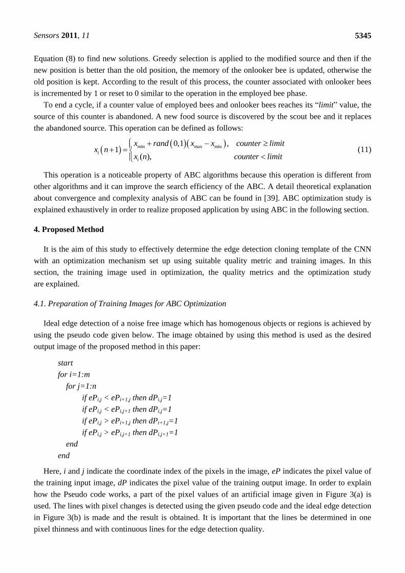
Here, i and j indicate the coordinate index of the pixels in the image, eP indicates the pixel value of

the training input image, dP indicates the pixel value of the training output image. In order to explain

how the Pseudo code works, a part of the pixel values of an artificial image given in Figure 3(a) is

used. The lines with pixel changes is detected using the given pseudo code and the ideal edge detection

in Figure 3(b) is made and the result is obtained. It is important that the lines be determined in one

pixel thinness and with continuous lines for the edge detection quality.

Sensors 2011, 11

5346

Figure 3. (a) A part of the input image (b) The ideal edge detected image.

A B

50

50

50

50

50

50

50

50

50

120

120

120

120

120

120

120

120

120

120

120

120

120120120120120120

180

180

180

180

180

180

180

180

180

180

180

180

180

180

180

180

180

180

180

180

180

180

180

180

180

180

180

180

180

180

180

180

180

180

180

180

180

180

180

180

180

180

180

180

180

180

180

180

180

180

180

180

180

180

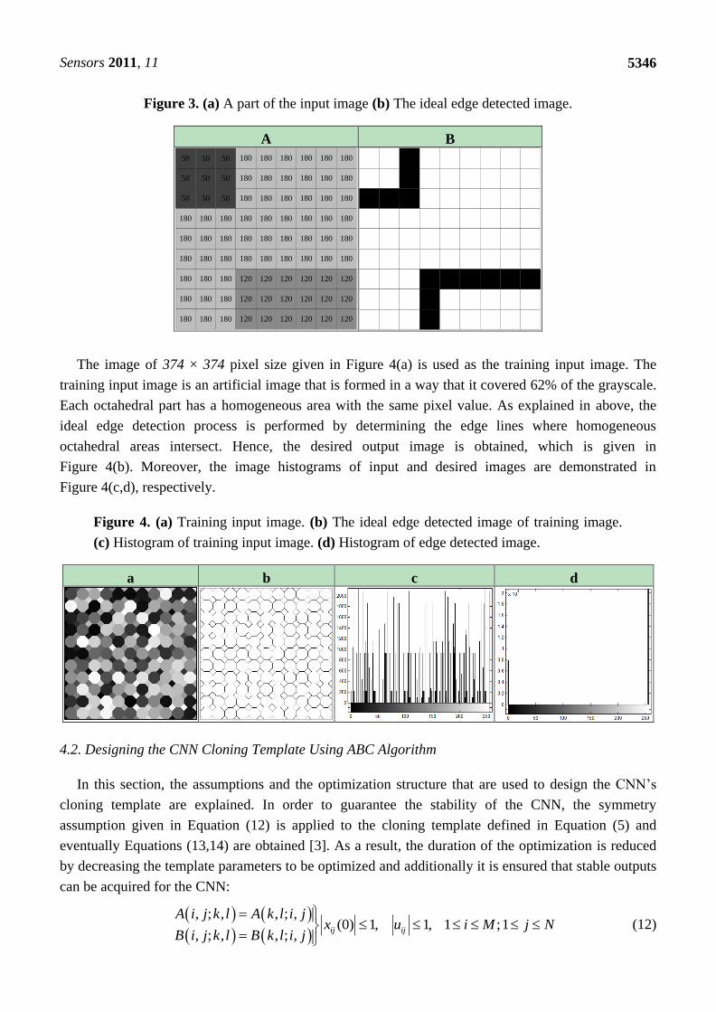
The image of 374 × 374 pixel size given in Figure 4(a) is used as the training input image. The

training input image is an artificial image that is formed in a way that it covered 62% of the grayscale.

Each octahedral part has a homogeneous area with the same pixel value. As explained in above, the

ideal edge detection process is performed by determining the edge lines where homogeneous

octahedral areas intersect. Hence, the desired output image is obtained, which is given in

Figure 4(b). Moreover, the image histograms of input and desired images are demonstrated in

Figure 4(c,d), respectively.

Figure 4. (a) Training input image. (b) The ideal edge detected image of training image.

(c) Histogram of training input image. (d) Histogram of edge detected image.

a b c d

4.2. Designing the CNN Cloning Template Using ABC Algorithm

In this section, the assumptions and the optimization structure that are used to design the CNN‟s

cloning template are explained. In order to guarantee the stability of the CNN, the symmetry

assumption given in Equation (12) is applied to the cloning template defined in Equation (5) and

eventually Equations (13,14) are obtained [3]. As a result, the duration of the optimization is reduced

by decreasing the template parameters to be optimized and additionally it is ensured that stable outputs

can be acquired for the CNN:

, ; , , ; ,(0) 1, 1, 1 ;1

, ; , , ; ,ij ij

A i j k l A k l i jx u i M j N

B i j k l B k l i j

(12)

Sensors 2011, 11

5347

1 2 3 1 2 3

4 5 4 4 5 4

3 2 1 3 2 1

a a a b b b

A a a a B b b b I z

a a a b b b

(13)

1 2 3, 4 5 1 2 3, 4 5, , , , , , , ,ix a a a a a b b b b b z (14)

The ABC design mechanism of the cloning template is shown in Figure 5. In this mechanism, the

output image of the CNN converges to the desired image by adjusting the cloning template of the CNN

by means of the ABC algorithm. The ABC algorithm produces template set and sends this set to the

the CNN. CNN runs by using this set and training image, and it generates an output image. The fitness

value of the objective function is calculated by comparing the output image of the CNN and the ideal

edge detected image. The ABC algorithm evaluates with this fitness value in order to obtain

better results.

Running of ABC optimization can be explained as follows: a D × SN size matrix is randomly

selected as the initial colony and each row of the matrix represents a cloning template set, a possible

solution to the problem, in the ABC optimization. D is the dimension of the problem and SN is the size

of the colony. There are three main phases in the ABC algorithm; the employed bees phase, the

onlooker bees phase and the scout bees phase.

Figure 5. Template design mechanism of the ABC based CNN edge detector.

The fitness value of each bee in the employed bee‟s colony (ne) is calculated by using Equation (16)

which is based on the correlation between output image of the CNN mechanism and the desired output

Figure 4(b). Local search is applied by Equation (10) at neighbors of all existing cloning templates. If

better fitness values are obtained after the local search process, these templates are included in the

population and the employed bees phase is completed. The onlooker bees phase is similar to the

previous phase. The only difference from the other is the operation of the local search mechanism.

This operation is not applied to all template sets, it is applied to some template set which is the

probability selected with the roulette wheel. Thus, the selection of the worse template is as much

possible as selection of a better template and therefore diversity in the population is ensured. If a

solution is not improved in both phases, the testing counter that is related with the solution is

incremented by 1, otherwise the counter reset to 0. In the scout bees phase, which template is removed

Sensors 2011, 11

5348

from population is arranged by controlling the testing counters by comparing these counters with the

parameter named “limit”. If the testing counter value of a template set reaches the limit value, this set

is removed from the population and a new cloning template set produced randomly is replaced instead

of the removed templates. All the explained processes are repeated as many times as indicated by the

as number of cycles of the ABC:

2 2

m n

i j

m n m n

i

ij ij

ij i

j

j

i j

z zPP tP tP

zP tP

C

zP tP

(15)

1

, 0 1if x rC ε

(16)

where i and j are pixel index on the image, zP is pixel value of the CNN output image, tP is pixel value

of the edge detected training image, is mean of the output image, is mean of the edge detected

training image, ε is a small positive constant, and f is objective function. The C value in Equation (16)

is the correlation between the two images and this is given in Equation (15).

By calculating the similarity between the output images of the CNN and the ideal edge detected

image, the optimization process is continued to prove better results by the ABC algorithm. Simulations

are developed on a MATLAB platform and the processing of the CNN structure is realized using the

MATCNN library [40,41].

4.3. The Simulation Results

The performance and robustness of ABC algorithm in determining the edge detecting CNN cloning

template are assessed statistically. The optimization results are obtained with multiple runs on different

control parameters of ABC; “limit” and the “size of colony” (NP), which are the control parameters of

ABC, are considered in the simulations [36].

In order to show the effect of the scout production mechanism on the performance of the algorithm,

the average of the best function values found for the different “limit” values (1 × ne × D, 2 × ne × D,

4 × ne × D and “without scout”) and colony sizes (20, 40 and 80) is given in Table 1. In the

simulations, the cycle and time step constant of the CNN are selected as 30 and 0.3, respectively.

Three thousand cycles are set for each combination of NP, and “limit” value and ABC is run

independently 30 times and the results obtained (f values in Equation (16)) are given in Table 1 as

mean (MEAN) and standard deviation (STD).

Table 1. The performance analysis results of ABC.

Colony NP = 20 (ne = no = 10) NP = 40 (ne = no = 20) NP = 80 (ne = no = 40)

Size Limit =

1×ne×D

Limit =

2×ne×D

Limit =

4×ne×D

Without

scout

Limit =

1×ne×D

Limit =

2×ne×D

Limit =

4×ne×D

Without

Scout

Limit =

1×ne×D

Limit =

2×ne×D

Limit =

4×ne×D

Without

scout

MEAN 0.7551 0.7340 0.7013 0.4525 0.7625 0.7450 0.7172 0.6483 0.7935 0.7509 0.7656 0.7048

STD 0.0517 0.0642 0.1660 0.2904 0.0643 0.0860 0.1057 0.2031 0.0521 0.0456 0.0483 0.1192

ne: number of employed bees, D: dimension of problem, runs = 30 and total evaluation number = 3,000.

Sensors 2011, 11

5349

In Table 1, it is seen that STD values are very low in all combinations of NP and “limit” values.

Therefore, it can be stated that the ABC optimization technique for this problem is quite a robust

algorithm. Moreover, the fact that the MEAN value gets smaller as the n value gets bigger supports the

assumption that choosing a smaller n value can lead to better results. Beside the results of Table 1, in

order to present a stable evaluation of the effect of control parameters of the ABC on its performance,

ANalysis Of the VAriance (ANOVA) based on the mean variance is used. ANOVA examines the

statistical difference of one, two or more groups over one quantitative one. The null hypothesis we

established for ANOVA is that all population means are equal and the other hypothesis is that at least

one mean is different from the others. Calculated F value is compared to the value coming from the F

distribution associated with the degrees of freedom and significance value. If this value is lower

than 0.05, the effect of the variable is considered to be statistically significant. ANOVA statistics are

calculated by using 12 different values of control parameters on MATLAB platform. Each data group

has 30 f values coming from each run. Results of ANOVA test for NP and limit control parameters are

presented in Table 2. In the table, each column presents values of the sum of squares (SS), the degrees

of freedom (df), Mean Squares (MS), which is the ratio SS/df and F statistics, which is the ratio of the

mean squares. From the results in Table 2, it can be said that f function is influenced significantly by

the values of NP and limit.

Table 2. ANOVA table for f function by 12 different control parameters of ABC.

Function SS df MS F Prob > F

f 2.65833 11 0.24167 14.21 1.22746e-022

At the values of MEAN = 0.7935 and STD = 0.0521 where optimization is at its best and most

effective, the population size and limit values are 80 and 440, respectively. The best C value obtained

so far is C = 0.9331 and the cloning template obtained that correspond to this value are presented in

Equation (17):

-0.2481 - 5.4392 -1.2947 -0.0051 0.0610 0.1331

A -7.3106 62.7200 -7.3106 B -0.0739 - 34.2720 -0.0739 I 1.6937

-1.2947 - 5.4392 -0.2481 0.1331 0.0610 -0.0051

(17)

The cloning template given in Equation (17) is the optimal template designed by the ABC algorithm

in this study for the purpose of edge detection.

4.4. Related Works

In this section, cloning templates of previous studies are presented and used to compare with the

ABC results. Designing the cloning template of CNN is an important task to achieve the desired results

and several technique-based analytic methods, local learning algorithms and heuristic methods are

proposed. Some of heuristic methods also used are Differential Evolution (DE) [27], Evolution

Strategies (ES) [28] techniques and Genetic Algorithm (GA) [22,32]. The first studies in the CNN area

were concentrated around binary images and later, some studies including gray-level images are

presented. Most template design studies do not include performance analyses of heuristic methods for

Sensors 2011, 11

5350

edge detection application and they are only introduced for design studies. In addition, templates

presented in previous studies are not compared subjectively and quantitatively with other templates

determined in the same area. Furthermore, edge detection studies based on CNN introduced without

applying threshold process with grayscale real images first are very limited. Therefore, there are

doubts about the reliability of heuristic methods in this kind of applications. In order to alleviate these

deficiencies, a performance analysis of the ABC is performed with multiple runs using its different

control parameters. The cloning template obtained with the ABC algorithm is compared subjectively

and quantitatively with other well-known techniques and previous studies on designing CNN cloning

templates. In the following tables, cloning templates determined in previous studies for edge detection

applications are presented. One of the presented cloning templates is from the MATCNN Template

Library (EDT-ML) [41]. The other cloning template is obtained by using the Differential Evolution

method (DE-CNN) [27]. Another cloning template is introduced by using Evolution Strategies

(ES-CNN) [28] and Xavier [29]. In the following sections, comparisons are made using these templates.

Table 3. Presented templates of previous studies based on CNN.

METHODS A

TEMPLATE

B

TEMPLATE

I

TEMPLATE

PARAMETER

OF CNN

ED-

TML[41]

0 0 0

0 2 0

0 0 0

-0.25 -0.25 -0.25

-0.25 2 -0.25

-0.25 -0.25 -0.25

−1.5 Time Step = 0.3

Iteration = 50

DE-

CNN[27]

5.9791 2.3636 5.9905

0.5346 14.8176 0.5346

5.9905 2.3636 5.9791

0.0304 0.0198 0.0049

0.0453 15.0325 0.0453

0.0049 0.0198 0.0304

1.1570 Time Step = 1.3937

Iteration = 2

ES-CNN[28]

0.0188 7.2196 1.6024

2.2306 20.8999 2.2306

1.6024 7.2196 0.0188

0.0397 0.3402 0.0362

0.2233 0.2497 0.2233

0.0362 0.3402 0.0397

−3.3014 Time Step = 0.3

Iteration = 20

Xavier[29]

0.2367 0.2416 0.2207

0.1710 1.8889 0.1710

0.2207 0.2416 0.2367

0.6522 0.0306 0.8290

0.0722 2.8511 0.0722

0.8290 0.0306 0.6522

−1.3631

Not given in the

paper, the values

used:

Time Step = 0.03

Iteration = 100

4.5. The Method of Comparison and Parameters

The edge detection quality of the templates in Equation (17), determined as a result of optimization,

is assessed by using both artificial binary and grayscale images, and real images. Edge detection is

performed on all images by using the well-known classical edge detector and the previously proposed

CNN based edge detectors and the novel CNN templates in Equation (17).

Firstly, subjective comparisons are presented in Figures 6–9. For better evaluation of these

subjective comparisons, the proposed method is given at the end of the rows of figures. The study is

continued with objective evaluation based on results of accepted comparison metrics.

Sensors 2011, 11

5351

Subjective comparisons of obtained cloning template and well-known edge detection methods by

use of the binary/grayscale artificial images are given in Figure 6.

Figure 6. Artificial images. (a) Text. (b) Shape. (c) Check. (d) Honeycomb. (e) Ledge [42].

a (600 × 600) b (600 × 600) c (100 × 100) d (115 × 115) e (256 × 256)

Ori

gin

al I

mag

es

Wel

l-K

now

n E

dge

Det

ecti

on

Met

hods

Wit

ho

ut

CN

N

Can

ny

Rober

ts

Pre

wit

t

Sobel

Pro

pose

d M

eth.

AB

C-C

NN

Figure 6(a) shows that all classic edge methods determined the ideal edges of the Text image

successfully. For the Shape image, as can be seen in Figure 6(b), it is seen that compared with the

proposed method the other methods are unsuccessful as indicated by the duplicate lines that occur in

the output edge image. It is obvious that for the gray-level artificial images, the Check, Honeycomb

and Ledge, as shown in Figure 6(c–e), respectively, the proposed method detected the edges as well as

the ideal edge detection, and, in fact is considerably more successful than well-known edge detection

Sensors 2011, 11

5352

methods. Subjective comparisons of obtained cloning template and previous studies based on CNN by

use of the binary/grayscale artificial images are given in Figure 7.

Figure 7. Artificial images. (a) Text. (b) Shape. (c) Check. (d) Honeycomb. (e) Ledge [42].

a (600 × 600) b (600 × 600) c (100 × 100) d (115 × 115) e (256 × 256)

O

rigin

al I

mag

es

Met

hods

Bas

ed o

n C

NN

ED

-TM

L

DE

-CN

N

ES

-CN

N

Xav

ier

AB

C-C

NN

Figure 7(a) shows that methods based on CNN, except for DE-CNN, determined the ideal edges of

the Text image successfully. For the Shape image, as can be seen in Figure 7(b), ES-CNN templates,

Xavier templates and ABC-CNN templates detects all boundaries as single lines. However the

DT-CNN method is unsuccessful as indicated by the duplicate lines that occur in the output edge

image and the results of the ED-TML method are unclear. It is obvious that for the gray-level artificial

images, the Check, Honeycomb and Ledge, as shown in Figure 7(c–e), respectively, the proposed

Sensors 2011, 11

5353

method detected the edges as well as the ideal and noiseless edge detection, and, in fact is considerably

more successful than other methods. Subjective comparisons of obtained cloning template and

well-known edge detection methods by use of the binary/grayscale real images are given in Figure 8.

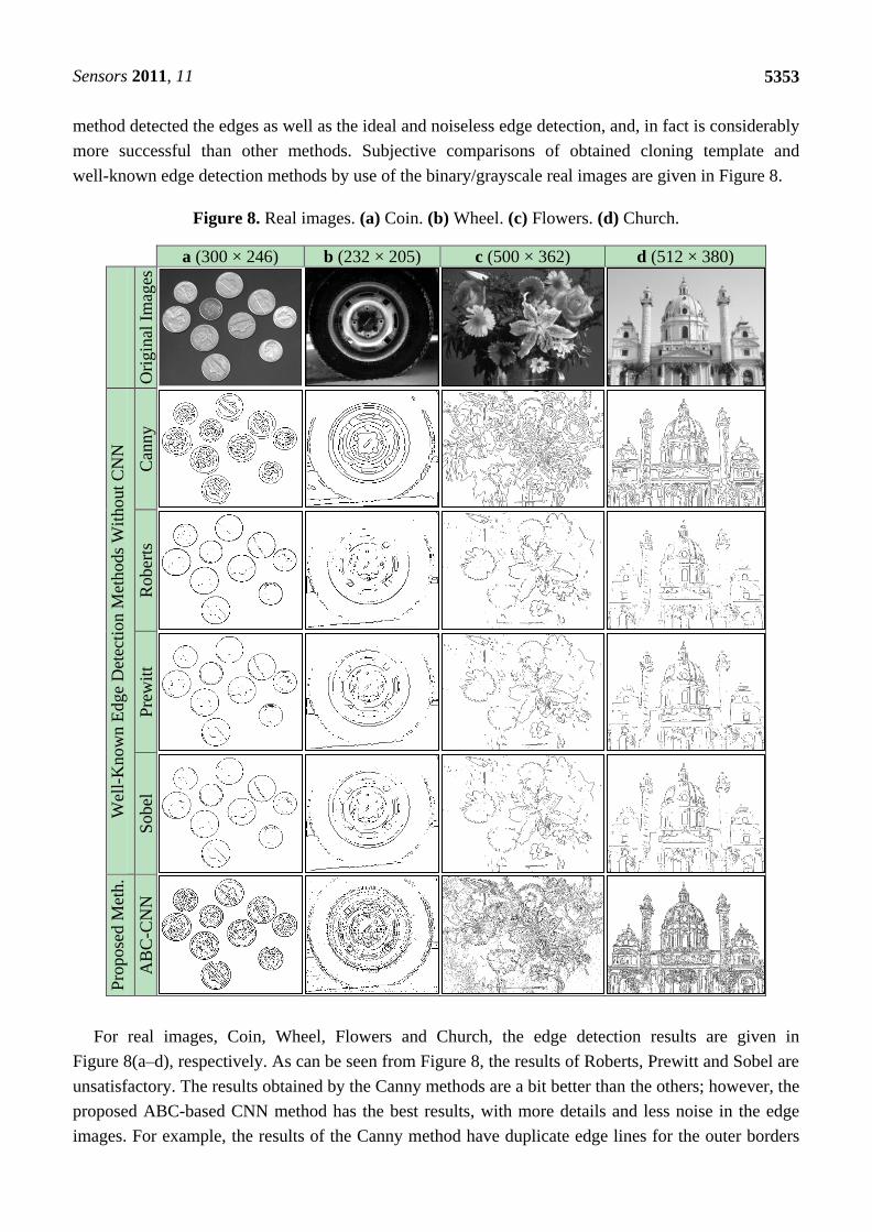
Figure 8. Real images. (a) Coin. (b) Wheel. (c) Flowers. (d) Church.

a (300 × 246) b (232 × 205) c (500 × 362) d (512 × 380)

Ori

gin

al I

mag

es

Wel

l-K

now

n E

dge

Det

ecti

on M

ethods

Wit

hout

CN

N

Can

ny

Rober

ts

Pre

wit

t

Sobel

Pro

pose

d M

eth.

AB

C-C

NN

For real images, Coin, Wheel, Flowers and Church, the edge detection results are given in

Figure 8(a–d), respectively. As can be seen from Figure 8, the results of Roberts, Prewitt and Sobel are

unsatisfactory. The results obtained by the Canny methods are a bit better than the others; however, the

proposed ABC-based CNN method has the best results, with more details and less noise in the edge

images. For example, the results of the Canny method have duplicate edge lines for the outer borders

Sensors 2011, 11

5354

of the coins in Figure 8(a) and loss of details for Figure 8(b–d). Subjective comparisons of obtained

cloning template and previous studies based on CNN by use of the binary/grayscale real images are

given in Figure 9.

Figure 9. Real images. (a) Coin. (b) Wheel. (c) Flowers. (d) Church.

a (300 × 246) b (232 × 205) c (500 × 362) d (512 × 380)

O

rigin

al I

mag

es

Met

hods

Bas

ed o

n C

NN

ED

-TM

L

DE

-CN

N

ES

-CN

N

Xav

ier

AB

C-C

NN

As can be seen the results of ED-TML are unsatisfactory. In the Xavier and ES-CNN method

results, the output images have too much noise, which reduces the perception of the edge detection

output. There are many undetected objects in the DE-CNN results, especially for Figure 9(b,c). It is

obvious that the results of the proposed ABC-based CNN method have more distinctive details than

other methods and less noise in the edge images.

Sensors 2011, 11

5355

Besides visual evaluation of the edge detection quality on binary and grayscale artificial images, it

is also the aim of the study to assess the edge detection quality quantitatively. For this reason, the

similarity between the results shown in Figures 6 and 7 and the ideal edge detection results given in

Figure 10 are compared.

Figure 10. The results of the ideal edge detection obtained using the ideal edge method.

a b c d e

Correlation (C), structural similarity (SSIM) [43] and mean squared error (MSE) values are used as

the comparison operators and results are presented in Table 4. To calculate the correlation, the

equation given in Equation (15) is used. Mean Squared Error (MSE) is given in Equation (18):

1 1

2

0 0

1, ,

m n

i j

MSE zP i j tP i jmn

(18)

where m × n is size of image, i and j are coordinate index of the pixels in the image. SSIM, which is

another similarity operator used for comparison, is given in Equation (19) [43]:

1 2

2 2 2 2

1 2

2 2

( )( )

zRtR

z

zR tR

zRR tR tR

μ μ c σ cSSIM

μ μ c σ σ c

(19)

2 2

1 1 2 2( ) , ( )c k L c k L (20)

Here, μzR, μtR are the mean gray-level intensity values of zR and tR images, respectively. and

are the variance of zR and tR images, respectively. σzRtR is the covariance of zR and tR images.

L is the dynamic interval of the pixel value and k1 and k2 are the constant numbers that are 0.01

and 0.03 [43].

Table 4. Comparison results of the detection methods with the results of ideal edge

detection for the binary and grayscale artificial images given in Figure 6.

TEXT SHAPE CHECK HONEYCOMP LEDGE

C MSE SSIM C MSE SSIM C MSE SSIM C MSE SSIM C MSE SSIM

CANNY 0.3393 1589.5 0.8733 0.0265 4254.3 0.6755 0.1922 20470 0.1774 0.3304 9228.9 0.3005 0.6393 5432.3 0.6335

ROBERTS 0.5062 1334.8 0.8951 0.6908 1048.3 0.9038 0.0867 21211 0.0532 0.2081 9568.1 0.1547 0.5281 6746.0 0.5432

PREWITT 0.4709 1260.0 0.8950 0.0260 4337.7 0.6806 0.0814 21055 0.0498 0.2001 9332.1 0.1484 0.5812 6163.6 0.5855

SOBEL 0.4602 1309.5 0.8929 0.0285 4300.5 0.6833 0.0805 21081 0.0493 0.2445 8973.2 0.1779 0.5819 6155.6 0.5859

ED-TML 0.9209 217.1 0.9855 0.0001 1456.4 0.7669 0.4428 15527 0.3411 0.4355 7154.3 0.2805 0.0324 9874.3 0.2507

DE-CNN 0.4545 4351.2 0.8914 0.5863 2607.0 0.7720 0.5736 14037 0.5946 0.5081 10093. 0.4975 0.3885 10060. 0.3500

ES-CNN 0.9632 94.6 0.9926 0.8735 436.0 0.9898 0.7461 7120 0.7693 0.7798 3456.5 0.8675 0.6382 5427.3 0.6819

XAVIER 0.9059 263.1 0.9825 0.8730 436.7 0.9899 0.7251 7547 0.7780 0.6224 5686.0 0.6947 0.5615 6356.8 0.6106

ABC-CNN 0.9754 62.0 0.9954 1.0000 0.0 1.0000 0.8609 4006 0.8614 0.8936 1622.6 0.9160 0.6610 5157.5 0.6768

Sensors 2011, 11

5356

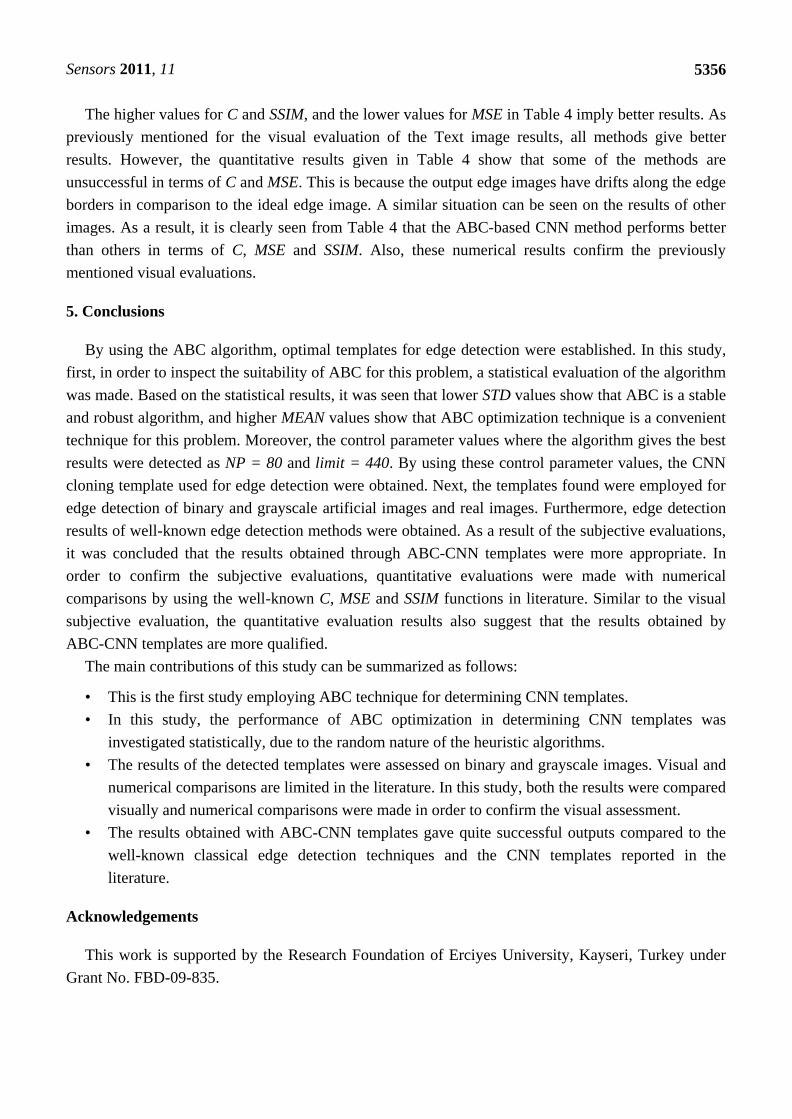
The higher values for C and SSIM, and the lower values for MSE in Table 4 imply better results. As

previously mentioned for the visual evaluation of the Text image results, all methods give better

results. However, the quantitative results given in Table 4 show that some of the methods are

unsuccessful in terms of C and MSE. This is because the output edge images have drifts along the edge

borders in comparison to the ideal edge image. A similar situation can be seen on the results of other

images. As a result, it is clearly seen from Table 4 that the ABC-based CNN method performs better

than others in terms of C, MSE and SSIM. Also, these numerical results confirm the previously

mentioned visual evaluations.

5. Conclusions

By using the ABC algorithm, optimal templates for edge detection were established. In this study,

first, in order to inspect the suitability of ABC for this problem, a statistical evaluation of the algorithm

was made. Based on the statistical results, it was seen that lower STD values show that ABC is a stable

and robust algorithm, and higher MEAN values show that ABC optimization technique is a convenient

technique for this problem. Moreover, the control parameter values where the algorithm gives the best

results were detected as NP = 80 and limit = 440. By using these control parameter values, the CNN

cloning template used for edge detection were obtained. Next, the templates found were employed for

edge detection of binary and grayscale artificial images and real images. Furthermore, edge detection

results of well-known edge detection methods were obtained. As a result of the subjective evaluations,

it was concluded that the results obtained through ABC-CNN templates were more appropriate. In

order to confirm the subjective evaluations, quantitative evaluations were made with numerical

comparisons by using the well-known C, MSE and SSIM functions in literature. Similar to the visual

subjective evaluation, the quantitative evaluation results also suggest that the results obtained by

ABC-CNN templates are more qualified.

The main contributions of this study can be summarized as follows:

• This is the first study employing ABC technique for determining CNN templates.

• In this study, the performance of ABC optimization in determining CNN templates was

investigated statistically, due to the random nature of the heuristic algorithms.

• The results of the detected templates were assessed on binary and grayscale images. Visual and

numerical comparisons are limited in the literature. In this study, both the results were compared

visually and numerical comparisons were made in order to confirm the visual assessment.

• The results obtained with ABC-CNN templates gave quite successful outputs compared to the

well-known classical edge detection techniques and the CNN templates reported in the

literature.

Acknowledgements

This work is supported by the Research Foundation of Erciyes University, Kayseri, Turkey under

Grant No. FBD-09-835.

Sensors 2011, 11

5357

References

1. Chua, L.O.; Yang, L. Cellular Neural Networks: Theory. IEEE Trans. Circ. Syst. Fund. Theor.

Appl. 1988, 35, 1257-1272.

2. Chua, L.O.; Yang, L. Cellular Neural Networks: Applications. IEEE Trans. Circ. Syst. Fund.

Theor. Appl. 1988, 35, 1273-1290.

3. Chua, L.O.; Roska, T. The CNN Paradigm. IEEE Trans. Circ. Syst. Fund. Theor. Appl. 1993, 40,

147-156.

4. Chua, L.O.; Roska, T. Cellular Neural Network and Visual Computing, 1st ed.; Cambridge

University Press: Cambridge, UK, 2002; pp. 35-50.

5. Matsumoto, T.; Chua, L.O.; Yokohama, T. Image Thinning with a Cellular Neural Network. IEEE

Trans. Circ. Syst. 1990, 37, 638-640.

6. Matsumoto, T.; Chua, L.O.; Suzuki, H. CNN Cloning Template: Shadow Detector. IEEE Trans.

Circ. Syst. 1990, 37, 1070-1073.

7. Crounse, K.R.; Chua, L.O. Methods for Image Processing in Cellular Neural Networks: A

Tutorial. IEEE Trans. Circ. Syst. 1995, 42, 583-601.

8. Venetianer, P.L.; Werblin, F.; Roska, T.; Chua, L.O. Analogic CNN Algorithms for Some Image

Compression and Restoration Tasks. IEEE Trans. Circ. Syst. Fund. Theor. Appl. 1995, 42,

278-284.

9. Julian, P.; Dogaru, R.; Chua, L.O. A Piecewise-Linear Simplicial Coupling Cell for CNN

Gray-Level Image Processing. IEEE Trans. Circ. Syst. 2002, 49, 904-913.

10. Gaobo, Y.; Zhaoyang, Z. Video Object Segmentation for Head-Shoulder Sequences in the

Cellular Neural Networks Architecture. Real-Time Imag. 2003, 9, 171-178.

11. Nishio, T.; Nishio, Y. Periodic Pattern Formation and Its Applications in Cellular Neural

Networks. IEEE Trans. Circ. Syst. 2008, 55, 2736-2742.

12. Gonzalez, R.C.; Wood, R.E.; Eddins, S.L. Digital Image Processing Using MATLAB, 2nd ed.;

Gatesmark Publishing: Knoxville, TN, USA, 2009; pp. 536-548.

13. Pratt, W.K. Digital Image Processing, 4th ed.; Wiley-Interscience: Malden, MA, USA, 2007;

pp. 465-534.

14. Yi, S.; Labate, D.; Easley, G.R.; Krim, H. A Shearlet Approach to Edge Analysis and Detection.

IEEE Trans. Image Process. 2009, 18, 929-941.

15. Lin, Z.; Jiang, J.; Wang, Z. Edge Detection in the Feature Space. Image Vision Comput. 2010, 29,

142-154.

16. Chua, L.O.; Thiran, P. An Analytic Method for Designing Simple Cellular Neural Network. IEEE

Trans. Circ. Syst. 1991, 38, 1332-1341.

17. Fajfar, I.; Bratkovic, F. Design of Monotonic Binary-Valued Cellular Neural Networks. In

Proceedings of IEEE International Workshop on Cellular Neural Networks and Their

Applications (CNNA’96), Seville, Spain, 24–26 June 1996; pp. 321-326.

18. Hanggi, M.; Moschytz, G.S. An Exact and Direct Analytical Method for the Design of Optimally

Robust CNN Templates. IEEE Trans. Circ. Syst. 1999, 46, 304-311.

19. Zarandy, A. The Art of Template Design. Int. J. Circ. Theor. Appl. 1998, 26, 5-23.

Sensors 2011, 11

5358

20. Zou, F.; Schwarz, S.; Nossek, J.A. Cellular Neural Network Design Using a Learning Algorithm.

In Proceedings of IEEE International Workshop on Cellular Neural Networks and Their

Applications (CNNA’90), Budapest, Hungary, 16–19 December 1990; pp. 73-81.

21. Tetzlaff, R.; Wolf, D. A Learning Algorithm for the Dynamics of CNN with Nonlinear Templates

Part I: Discrete-Time Case. In Proceedings of IEEE International Workshop on Cellular Neural

Networks and Their Applications (CNNA’96), Seville, Spain, 24–26 June 1996; pp. 461-466.

22. Kozek, T.; Roska, T.; Chua, L.O. Genetic Algorithm for CNN Template Learning. IEEE Trans.

Circ. Syst. Fund. Theor. Appl. 1993, 40, 392-402.

23. Shou, Y.W.; Lin, C.T. Image Descreening by GA-CNN Based Texture Classification. IEEE Trans.

Circ. Syst. 2004, 51, 2287-2299.

24. Pham, D.T.; Karaboga, D. Intelligent Optimization Techniques, 1st ed.; Springer: London, UK,

2000; pp. 1-299.

25. Chang, C.L.; Fan, K.W.; Chung, I.F.; Lin, C.T. A Recurrent Fuzzy Coupled Cellular Neural

Network System with Automatic Structure and Template Learning. IEEE Trans. Circ. Syst. 2006,

53, 602-606.

26. Giaquinto, A.; Fornarelli, G. PSO-Based Cloning Template Design for CNN Associative

Memories. IEEE Trans. Neural Netw. 2009, 20, 1837-1841.

27. Basturk, A.; Gunay, E. Efficient Edge Detection in Digital Images Using a Cellular Neural

Network Optimized by Differential Evolution Algorithm. Expert Syst. Appl. 2009, 36, 2645-2650.

28. Parmaksizoglu, S.; Alci, M. Designing CNN Templates for Edge Detection by Using Evolution

Strategies. In Proceedings of International Symposium on Innovations in Intelligent Systems and

Applications, Kayseri, Turkey, June 2010; pp. 396-399.

29. Xavier-de-Souza, S.; Yalcin, M.E.; Suykens, J.A.K.; Vandewalle, J. Toward CNN Chip-Specific

Robustness. IEEE Trans. Circ. Syst. Fund. Theor. Appl. 2004, 51, 892-902.

30. Lu, Z.; Liu, D. Design of Cellular Neural Networks with Space-Invariant Cloning Template. In

Proceedings of the IEEE International Symposium on Circuits and Systems, Monterey, CA, USA,

31 May–3 June 1998; pp. 215-218.

31. Yin, C.-L.; Wan, J.-L.; Lin, H.; Chen, W.-K. The Cloning Template Design of a Cellular Neural

Network. Brief Commun. 1999, 336, 903-909.

32. Khan, U.-A.; Fasih, A.; Kyamakya, K.; Chedjou, J.-C. Genetic Algorithm Based Template

Optimization for Vision System: Obstacle Detection. In Proceedings of International Symposium

on Theoretical Electrical Engineering, Lübeck, Germany, 22–24 June 2009; pp. 164-168.

33. Su, T.-J.; Huang, M.-Y.; Hou, C.-L.; Lin, Y.-J. Cellular Neural Networks for Gray Image Noise

Cancellation Based on a Hybrid Linear Matrix Inequality and Particle Swarm Optimization

Approach. Neural Process. Lett. 2010. 32, 147-165.

34. Karaboga, D. An Idea Based On Honey Bee Swarm for Numerical Optimization; Technical

Report-TR06; Computer Engineering Department, Erciyes University: Kayseri, Turkey, 2005.

35. Kurban, T.; Beşdok, E. A Comparison of RBF Neural Network Training Algorithms for Inertial

Sensor Based Terrain Classification. Sensors 2009, 9, 6312-6329.

36. Karaboga, D.; Basturk, B. A Powerful and Efficient Algorithm for Numerical Function

Optimization: Artificial Bee Colony (ABC) Algorithm. J. Global Optim. 2007, 39, 459-471.

Sensors 2011, 11

5359

37. Karaboga, D.; Basturk, B. On the Performance of Artificial Bee Colony (ABC) Algorithm. Appl.

Soft Comput. 2008, 8, 687-697.

38. Karaboga, D.; Basturk, B. A Comparative Study of Artificial Bee Colony Algorithm. Appl. Math.

Comput. 2009, 214, 108-132.

39. Xu, C.; Duan, H. Artificial Bee Colony (ABC) Optimized Edge Potential Function (EPF)

Approach to Target Recognition for Low-altitude Aircraft. Pattern Recogn. Lett. 2010, 31,

1759-1772.

40. Artificial Bee Colony (ABC) Algorithm Homepage. Available online: http://mf.erciyes.edu.tr/abc/

software.htm (accessed on 1 April 2011).

41. MATCNN: Analogical CNN Simulation Toolbox for MATLAB; Hungarian Academy of Science:

Budapest, Hungary; Available online: http://lab.analogic.sztaki.hu/ (accessed on 1 April 2011).

42. Ledge Test Image. Available online: http://w3.ualg.pt/~dubuf/pubdat/ledge/ledge.html (accessed

on 1 April 2011).

43. Wang, Z.; Bovik, A.C.; Sheikh, H.R.; Simoncelli, E.P. Image Quality Assessment: From Error

Visibility to Structural Similarity. IEEE Trans. Image Process. 2004, 13, 600-612.

© 2011 by the authors; licensee MDPI, Basel, Switzerland. This article is an open access article

distributed under the terms and conditions of the Creative Commons Attribution license

(http://creativecommons.org/licenses/by/3.0/).