C:My DocumentsDoc in...
147
AQWA-DRIFT MANUAL PREFACE The development of the AQWA suite of programs was carried out by Century Dynamics Limited who are continually improving the capabilities of the programs, as more advanced hydrodynamic calculation techniques become available. Century Dynamics Limited welcome suggestions from users regarding program development. Century Dynamics Limited Dynamics House 86, Hurst Road Horsham, West Sussex RH12 2DT Tel: +44 (0)1403 270066 Fax: +44 (0)1403 270099
Transcript of C:My DocumentsDoc in...

AQWA-DRIFTMANUAL
PREFACE
The development of the AQWA suite of programs was carried out by Century Dynamics Limitedwho are continually improving the capabilities of the programs, as more advanced hydrodynamiccalculation techniques become available.
Century Dynamics Limited welcome suggestions from users regarding program development.
Century Dynamics LimitedDynamics House
86, Hurst RoadHorsham, West Sussex
RH12 2DT
Tel: +44 (0)1403 270066Fax: +44 (0)1403 270099

Contents
AQWA-DRIFT User Manual 02 Page i
C O N T E N T S
CHAPTER 1 - INTRODUCTION . . . . . . . . . . . . . . . . . . . . . . . . . . . . . . . . . . . . Page 1 - 1421.1 PROGRAM . . . . . . . . . . . . . . . . . . . . . . . . . . . . . . . . . . . . . . . . . . . . Page 1 - 1421.2 MANUAL . . . . . . . . . . . . . . . . . . . . . . . . . . . . . . . . . . . . . . . . . . . . . Page 1 - 142
CHAPTER 2 - PROGRAM DESCRIPTION . . . . . . . . . . . . . . . . . . . . . . . . . . . . Page 1 - 1422.1 PROGRAM CAPABILITY . . . . . . . . . . . . . . . . . . . . . . . . . . . . . . . . Page 1 - 1422.2 THE COMPUTER PROGRAM . . . . . . . . . . . . . . . . . . . . . . . . . . . . . Page 3 - 142
CHAPTER 3 - THEORETICAL FORMULATION . . . . . . . . . . . . . . . . . . . . . . . Page 1 - 1423.1 HYDROSTATIC LOADING . . . . . . . . . . . . . . . . . . . . . . . . . . . . . . . Page 6 - 142
3.1.1 Hydrostatic Forces and Moments . . . . . . . . . . . . . . . . . . Page 6 - 1423.1.2 Hydrostatic Equilibrium . . . . . . . . . . . . . . . . . . . . . . . . . . Page 6 - 1423.1.3 Hydrostatic Stiffness Matrix . . . . . . . . . . . . . . . . . . . . . . Page 7 - 1423.2.1 Morison Forces . . . . . . . . . . . . . . . . . . . . . . . . . . . . . . . . Page 9 - 142
3.3 DIFFRACTION/RADIATION WAVE FORCES . . . . . . . . . . . . . . Page 10 - 1423.4 MEAN WAVE DRIFT FORCES . . . . . . . . . . . . . . . . . . . . . . . . . . . Page 11 - 1423.5 SLOWLY VARYING WAVE DRIFT FORCES . . . . . . . . . . . . . . Page 12 - 1423.6 INTERACTIVE FLUID LOADING BETWEEN BODIES . . . . . . Page 13 - 1423.7 STRUCTURAL ARTICULATIONS AND CONSTRAINTS . . . . . Page 15 - 142
3.7.1 Articulations . . . . . . . . . . . . . . . . . . . . . . . . . . . . . . . . . . Page 15 - 1423.7.2 Constraints . . . . . . . . . . . . . . . . . . . . . . . . . . . . . . . . . . . Page 15 - 142
3.8 WIND AND CURRENT LOADING . . . . . . . . . . . . . . . . . . . . . . . . Page 16 - 1423.8.1 Wind and Current . . . . . . . . . . . . . . . . . . . . . . . . . . . . . . Page 16 - 1423.8.2 Yaw Rate Drag Force . . . . . . . . . . . . . . . . . . . . . . . . . . . Page 16 - 142
3.9 THRUSTER FORCES . . . . . . . . . . . . . . . . . . . . . . . . . . . . . . . . . . . Page 18 - 1423.10 MOORING LINES . . . . . . . . . . . . . . . . . . . . . . . . . . . . . . . . . . . . . . Page 19 - 142
3.10.1 Force of Constant Magnitude and Direction . . . . . . . . . Page 19 - 1423.10.2 Constant Tension Winch Line . . . . . . . . . . . . . . . . . . . . Page 19 - 1423.10.3 Weightless Elastic Hawsers . . . . . . . . . . . . . . . . . . . . . . Page 19 - 1423.10.4 Heavy Inelastic Catenary Chains . . . . . . . . . . . . . . . . . . Page 20 - 1423.10.5 Translation of the Mooring Line Force and Stiffness
Matrix . . . . . . . . . . . . . . . . . . . . . . . . . . . . . . . . . . . . . . Page 22 - 1423.10.6 Stiffness Matrix for a Mooring Line Joining Two
Structures . . . . . . . . . . . . . . . . . . . . . . . . . . . . . . . . . . . . Page 23 - 1423.11 WAVE SPECTRA . . . . . . . . . . . . . . . . . . . . . . . . . . . . . . . . . . . . . . Page 24 - 1423.12 STABILITY ANALYSIS . . . . . . . . . . . . . . . . . . . . . . . . . . . . . . . . . Page 24 - 1423.13 FREQUENCY DOMAIN SOLUTION . . . . . . . . . . . . . . . . . . . . . . Page 24 - 1423.14 TIME HISTORY SOLUTION IN IRREGULAR WAVES . . . . . . . Page 25 - 142
3.14.1 Time Integration of Equation of Motion . . . . . . . . . . . . Page 25 - 1423.14.2 Motions at Drift Frequency . . . . . . . . . . . . . . . . . . . . . . Page 25 - 1423.14.3 Motions at Drift and Wave Frequency . . . . . . . . . . . . . . Page 26 - 1423.14.4 Slow Drift and Wave Frequency Positions . . . . . . . . . . Page 27 - 1423.14.5 Response Amplitude Operator Based Position . . . . . . . Page 28 - 142

Contents
AQWA-DRIFT User Manual 02 Page ii
3.14.6 Filtering of Slow Position from Total Position . . . . . . . Page 29 - 1423.14.7 Initial Position and Transients . . . . . . . . . . . . . . . . . . . . Page 29 - 142
3.15 TIME HISTORY SOLUTION IN REGULAR WAVES . . . . . . . . . Page 30 - 1423.16 LIMITATIONS OF THEORETICAL APPLICATIONS . . . . . . . . Page 30 - 1423.17 THE USE OF CONVOLUTION FOR THE EVALUATION OF THE
RADIATION FORCES IN THE TIME-DOMAIN . . . . . . . . . . . . . Page 30 - 142
CHAPTER 4 - MODELLING TECHNIQUES . . . . . . . . . . . . . . . . . . . . . . . . . . Page 33 - 1424.1 INTRODUCTION . . . . . . . . . . . . . . . . . . . . . . . . . . . . . . . . . . . . . . Page 34 - 1424.2 MODELLING REQUIREMENTS FOR AQWA-DRIFT . . . . . . . . Page 35 - 142
4.2.1 When Used as an Independent Program . . . . . . . . . . . . Page 35 - 1424.2.2 Following an AQWA-LINE Run . . . . . . . . . . . . . . . . . . Page 35 - 142
4.3 DEFINITION OF STRUCTURE AND POSITION . . . . . . . . . . . . Page 36 - 1424.3.1 Axis Systems . . . . . . . . . . . . . . . . . . . . . . . . . . . . . . . . . Page 36 - 1424.3.2 Conventions . . . . . . . . . . . . . . . . . . . . . . . . . . . . . . . . . . Page 36 - 1424.3.3 The Structural Definition and Analysis Position . . . . . . Page 37 - 142
4.4 STRUCTURE GEOMETRY AND MASS DISTRIBUTION . . . . . Page 38 - 1424.4.1 Coordinates . . . . . . . . . . . . . . . . . . . . . . . . . . . . . . . . . . Page 38 - 1424.4.2 Elements and Element Properties . . . . . . . . . . . . . . . . . . Page 38 - 142
4.5 MORISON ELEMENTS . . . . . . . . . . . . . . . . . . . . . . . . . . . . . . . . . Page 39 - 1424.5.1 Reynolds Number Dependent Drag Coefficients . . . . . . Page 39 - 1424.5.2 Morison Forces For AQWA-DRIFT with no Wave
Frequency Motions . . . . . . . . . . . . . . . . . . . . . . . . . . . . Page 40 - 1424.6 STATIC ENVIRONMENT . . . . . . . . . . . . . . . . . . . . . . . . . . . . . . . Page 41 - 142
4.6.1 Global Environmental Parameters . . . . . . . . . . . . . . . . . Page 41 - 1424.7 LINEAR STIFFNESS . . . . . . . . . . . . . . . . . . . . . . . . . . . . . . . . . . . Page 42 - 142
4.7.1 Hydrostatic Stiffness . . . . . . . . . . . . . . . . . . . . . . . . . . . Page 42 - 1424.7.2 Additional Linear Stiffness . . . . . . . . . . . . . . . . . . . . . . Page 42 - 142
4.8 WAVE FREQUENCIES AND DIRECTIONS . . . . . . . . . . . . . . . . Page 43 - 1424.9 WAVE LOADING COEFFICIENTS . . . . . . . . . . . . . . . . . . . . . . . Page 44 - 1424.10 WIND AND CURRENT LOADING COEFFICIENTS . . . . . . . . . Page 45 - 1424.11 THRUSTER FORCES . . . . . . . . . . . . . . . . . . . . . . . . . . . . . . . . . . . Page 45 - 1424.12 CONSTRAINTS OF STRUCTURE MOTIONS . . . . . . . . . . . . . . . Page 45 - 1424.13 STRUCTURAL ARTICULATIONS . . . . . . . . . . . . . . . . . . . . . . . . Page 46 - 142
4.13.1 Articulations . . . . . . . . . . . . . . . . . . . . . . . . . . . . . . . . . . Page 46 - 1424.13.2 Constraints . . . . . . . . . . . . . . . . . . . . . . . . . . . . . . . . . . . Page 46 - 142
4.14 WAVE SPECTRA, WIND AND CURRENT SPECIFICATION . . Page 47 - 1424.15 MOORING LINES . . . . . . . . . . . . . . . . . . . . . . . . . . . . . . . . . . . . . . Page 48 - 142
4.15.1 Linear/Non-Linear Elastic Hawsers . . . . . . . . . . . . . . . . Page 48 - 1424.15.2 Constant Tension Winch Line . . . . . . . . . . . . . . . . . . . . Page 49 - 1424.15.3 ‘Constant Force’ Line . . . . . . . . . . . . . . . . . . . . . . . . . . Page 49 - 1424.15.4 Catenary line . . . . . . . . . . . . . . . . . . . . . . . . . . . . . . . . . Page 49 - 1424.15.5 Steel Wire Cables . . . . . . . . . . . . . . . . . . . . . . . . . . . . . . Page 50 - 1424.15.6 Intermediate Buoys and Clump Weights . . . . . . . . . . . . Page 50 - 1424.15.7 The Pulley Card (PULY) . . . . . . . . . . . . . . . . . . . . . . . . Page 50 - 1424.15.8 The Drum Winch (LNDW) . . . . . . . . . . . . . . . . . . . . . . Page 50 - 1424.15.9 Fenders (FEND) . . . . . . . . . . . . . . . . . . . . . . . . . . . . . . . Page 50 - 142

Contents
AQWA-DRIFT User Manual 02 Page iii
4.16 ITERATION PARAMETERS FOR SOLUTION OF EQUILIBRIUM (AQWA-LIBRIUM ONLY) . . . . . . . . . . . . . . . . . Page 51 - 142
4.17 TIME HISTORY INTEGRATION IN IRREGULAR WAVES . . . Page 52 - 1424.17.1 Timestep for Simulation . . . . . . . . . . . . . . . . . . . . . . . . . Page 52 - 1424.17.2 Simulation Length and Accuracy Limits . . . . . . . . . . . . Page 52 - 1424.17.3 Initial Conditions and Start Time . . . . . . . . . . . . . . . . . . Page 54 - 142
4.18 TIME HISTORY INTEGRATION IN REGULAR WAVES(AQWA-NAUT ONLY) . . . . . . . . . . . . . . . . . . . . . . . . . . . . . . . . . Page 55 - 142
4.19 SPECIFICATION OF OUTPUT REQUIREMENTS . . . . . . . . . . . Page 55 - 142
CHAPTER 5 - ANALYSIS PROCEDURE . . . . . . . . . . . . . . . . . . . . . . . . . . . . . Page 56 - 1425.1 TYPES OF ANALYSIS . . . . . . . . . . . . . . . . . . . . . . . . . . . . . . . . . . Page 57 - 1425.2 RESTART STAGES . . . . . . . . . . . . . . . . . . . . . . . . . . . . . . . . . . . . Page 57 - 1425.3 STAGES OF ANALYSIS . . . . . . . . . . . . . . . . . . . . . . . . . . . . . . . . Page 58 - 142
CHAPTER 6 - DATA REQUIREMENT AND PREPARATION . . . . . . . . . . . Page 60 - 1426.0 ADMINISTRATION CONTROL - DECK 0 - PRELIMINARY
DECK . . . . . . . . . . . . . . . . . . . . . . . . . . . . . . . . . . . . . . . . . . . . . . . Page 61 - 1426.1 STAGE 1 - DECKS 1 TO 5 - GEOMETRIC DEFINITION AND
STATIC ENVIRONMENT . . . . . . . . . . . . . . . . . . . . . . . . . . . . . . . Page 63 - 1426.1.1 Description Summary of Physical Parameters Input . . Page 63 - 1426.1.2 Description of General Format . . . . . . . . . . . . . . . . . . . . Page 63 - 1426.1.3 Data Input Summary for Decks 1 to 5 . . . . . . . . . . . . . . Page 64 - 142
6.2 STAGE 2 - DECKS 6 TO 8 - THE DIFFRACTION/RADIATION ANALYSIS PARAMETERS . . . . . . . . . . . . . . . . . . . . . . . . . . . . . Page 65 - 1426.2.1 Description Summary of Physical Parameters Input . . . Page 65 - 1426.2.2 Description of General Format . . . . . . . . . . . . . . . . . . . . Page 65 - 1426.2.3 Total Data Input Summary for Decks 6 to 8 . . . . . . . . . Page 66 - 1426.2.4 Input for AQWA-DRIFT using the Results of a Previous
AQWA-LINE Run . . . . . . . . . . . . . . . . . . . . . . . . . . . . . Page 67 - 1426.2.5 Input for AQWA-DRIFT with Results from a Source
other than AQWA-LINE . . . . . . . . . . . . . . . . . . . . . . . . Page 67 - 1426.2.6 Input for AQWA-DRIFT with Results from a Previous
AQWA-LINE Run and a Source other than AQWA-LINE . . . . . . . . . . . . . . . . . . . . . . . . . . . . . . . . . Page 68 - 142
6.3 STAGE 3 - NO CARD IMAGE INPUT - DIFFRACTION/RADIATION ANALYSIS . . . . . . . . . . . . . . . . . . . . . . . . . . . . . . . . Page 69 - 142
6.4 Stage 4 - DECKS 9 to 18 - INPUT OF THE ANALYSIS ENVIRONMENT . . . . . . . . . . . . . . . . . . . . . . . . . . . . . . . . . . . . . . . Page 70 - 1426.4.1 Description Summary of Parameters Input . . . . . . . . . . Page 70 - 1426.4.2 AQWA-DRIFT Data Input Summary for Decks 9 to 18 Page 71 - 142
6.5 STAGE 5 - NO INPUT - Motion Analysis . . . . . . . . . . . . . . . . . . . Page 72 - 1426.6 STAGE 6 - NO DECKS - GRAPHICAL DISPLAY . . . . . . . . . . . . Page 72 - 142
6.6.1 Input for Display of Model and Results . . . . . . . . . . . . . Page 72 - 142
CHAPTER 7 - DESCRIPTION OF OUTPUT . . . . . . . . . . . . . . . . . . . . . . . . . . Page 73 - 1427.1 STRUCTURAL DESCRIPTION OF BODY CHARACTERISTICS

Contents
AQWA-DRIFT User Manual 02 Page iv
. . . . . . . . . . . . . . . . . . . . . . . . . . . . . . . . . . . . . . . . . . . . . . . . . . . . . Page 74 - 1427.1.1 Coordinates and Mass Distribution Elements . . . . . . . . Page 74 - 142
7.2 DESCRIPTION OF ENVIRONMENT . . . . . . . . . . . . . . . . . . . . . . Page 78 - 1427.3 DESCRIPTION OF FLUID LOADING . . . . . . . . . . . . . . . . . . . . . Page 80 - 142
7.3.1 Hydrostatic Stiffness . . . . . . . . . . . . . . . . . . . . . . . . . . . Page 80 - 1427.3.2 Added Mass and Wave Damping . . . . . . . . . . . . . . . . . . Page 81 - 1427.3.3 Oscillatory Wave Excitation Forces . . . . . . . . . . . . . . . Page 82 - 1427.3.4 Mean Wave Drift Forces . . . . . . . . . . . . . . . . . . . . . . . . Page 84 - 142
7.4 FREE FLOATING NATURAL FREQUENCIES AND RESPONSE AMPLITUDE OPERATORS . . . . . . . . . . . . . . . . . . . Page 85 - 1427.4.1 Natural Frequencies/Periods . . . . . . . . . . . . . . . . . . . . . Page 85 - 1427.4.2 Response Amplitude Operators . . . . . . . . . . . . . . . . . . . Page 86 - 142
7.5 SPECTRAL LINE PRINTOUT . . . . . . . . . . . . . . . . . . . . . . . . . . . . Page 88 - 1427.6 TIME HISTORY AND FORCE PRINTOUT . . . . . . . . . . . . . . . . . Page 89 - 1427.7 STATISTICS PRINTOUT . . . . . . . . . . . . . . . . . . . . . . . . . . . . . . . . Page 94 - 142
CHAPTER 8 - EXAMPLE OF PROGRAM USE . . . . . . . . . . . . . . . . . . . . . . . . Page 96 - 1428.1 BOX STRUCTURE . . . . . . . . . . . . . . . . . . . . . . . . . . . . . . . . . . . . . Page 97 - 142
8.1.1 General Discussion . . . . . . . . . . . . . . . . . . . . . . . . . . . . Page 97 - 1428.1.2 Problem Definition . . . . . . . . . . . . . . . . . . . . . . . . . . . . . Page 97 - 1428.1.3 Natural Frequencies . . . . . . . . . . . . . . . . . . . . . . . . . . . Page 100 - 1428.1.4 Low Frequency Added Mass and Damping . . . . . . . . . Page 101 - 1428.1.5 Hull and Superstructure Loading Coefficients . . . . . . . Page 101 - 1428.1.6 Sea Spectra, Current and Wind . . . . . . . . . . . . . . . . . . Page 102 - 1428.1.7 Specification of the Mooring Lines . . . . . . . . . . . . . . . Page 103 - 1428.1.8 Start Position for Analysis . . . . . . . . . . . . . . . . . . . . . . Page 103 - 1428.1.9 Time Integration Parameters . . . . . . . . . . . . . . . . . . . . Page 103 - 1428.1.10 Input Preparation For Natural Frequency Data Run . . Page 104 - 1428.1.11 Output from Natural Frequency Data Run . . . . . . . . . . Page 107 - 1428.1.12 Natural Frequency Simulation Run . . . . . . . . . . . . . . . Page 117 - 1428.1.13 Output from Natural Frequency Run . . . . . . . . . . . . . . Page 117 - 1428.1.14 Input Preparation for Drift Motion Data Run . . . . . . . Page 121 - 1428.1.15 Drift Motion Simulation Run . . . . . . . . . . . . . . . . . . . . Page 123 - 1428.1.16 Output from Drift Motion Simulation Run . . . . . . . . . Page 124 - 1428.1.17 Input for Drift/Wave Frequency Simulation Run . . . . Page 128 - 1428.1.18 Output from Drift/Wave Frequency Simulation Run . . Page 130 - 142
CHAPTER 9 - RUNNING THE PROGRAM . . . . . . . . . . . . . . . . . . . . . . . . . . Page 133 - 1429.1 Running AQWA-DRIFT on the PC . . . . . . . . . . . . . . . . . . . . . . . . Page 134 - 142
9.1.1 File Naming Convention for AQWA Files . . . . . . . . . Page 134 - 1429.1.2 AQWA File Organisation . . . . . . . . . . . . . . . . . . . . . . Page 135 - 1429.1.3 Program Size Requirements . . . . . . . . . . . . . . . . . . . . . Page 135 - 1429.1.4 Run Commands . . . . . . . . . . . . . . . . . . . . . . . . . . . . . . Page 136 - 142
APPENDIX A - AQWA-DRIFT PROGRAM OPTIONS . . . . . . . . . . . . . . . . . Page 137 - 142
APPENDIX B - REFERENCES . . . . . . . . . . . . . . . . . . . . . . . . . . . . . . . . . . . . Page 142 - 142

Introduction
AQWA-DRIFT User Manual 02 Page 1 - 142
CHAPTER 1 - INTRODUCTION
1.1 PROGRAM
AQWA-DRIFT is a computer program which simulates the motion of floating structuresarbitrarily connected by articulations or mooring lines under the action of wind, wave andcurrent forces. The program has the following two modes of operation:
1. Slow drift mode, in which the structure is subjected to only the second order waveforces, steady wind and current;
2. Wave frequency mode, in which both slow drift and wave frequency forces areincluded along with steady wind and current.
The program requires a full hydrostatic and hydrodynamic description of each structure. This caneither be input as data or transferred directly from the output results of an AQWA-LINEanalysis.
1.2 MANUAL
The AQWA-DRIFT Program Manual describes the various uses of the program together withthe method of operation. The theory and bounds of application are outlined for the analyticalprocedures employed within the various parts of AQWA-DRIFT.
The method of data preparation and modelling is fully described and reference is made to theAQWA Reference Manual. The Reference Manual contains information common to one or moreprograms and a complete guide to the format used for input of data into the AQWA Suite. It isdesirable that the AQWA-DRIFT Program Manual and AQWA Reference Manual be availablewhen using the program AQWA-DRIFT.
Program Description
AQWA-DRIFT User Manual 02 Page 2 - 142
CHAPTER 2 - PROGRAM DESCRIPTION
AQWA-DRIFT is a time domain program which uses linear hydrodynamic coefficients suppliedby AQWA-LINE or an equivalent source of linear hydrodynamic data plus other hydrodynamicand hydrostatic information to simulate the motions of large floating structures.
2.1 PROGRAM CAPABILITY
AQWA-LINE computes the linearised hydrodynamic fluid wave loading on a floating or fixedrigid body using 3-dimensional diffraction/radiation theory. The fluid forces are composed ofreactive forces and active excitation forces. The reactive fluid loading is due to body motions andmay be calculated by investigating the radiated wave field arising from body motions. The activeor excitation loading which induces motion, is composed of diffraction forces due to thescattering of the incident wave field, and the Froude-Krylov force due to the pressure field in theundisturbed incident wave.
The incident wave acting on the body is assumed to be harmonic and of small amplitudecompared to its wavelength. To calculate the hydrodynamic coefficients, the fluid is assumed tobe ideal and hence potential flow theory is used. Effects which are attributable to the viscosityof the fluid are taken into account in the calculation of the current loads and other hull forces.The hydrostatic fluid forces may also be calculated using AQWA-LINE and these, whencombined with the hydrodynamic forces and body mass characteristics, may be used to calculatethe small amplitude rigid body response about a mean position. The mean second order wavedrift forces may also be calculated by AQWA-LINE after the first order fluid flow problem hasbeen solved. These are used by AQWA-DRIFT to calculate the slowly varying drift force oneach structure. The drift force is calculated at each timestep in the simulation, together with theinstantaneous value of all other forces. These are applied to the structure, and the resultingacceleration calculated. From this, the position and velocity are determined at the subsequenttimestep. The process is then repeated at the following timestep, and so the time history of thestructure motion is constructed. The program can be used to calculate the response of structuresto drift forces only, but wave forces can also be added with the restriction that the length of timebetween calculation of the forces and integration of the structure motions must be decreased toaccommodate the more rapid variation in wave force.
Program Description
AQWA-DRIFT User Manual 02 Page 3 - 142
2.2 THE COMPUTER PROGRAM
The program AQWA-DRIFT may be used on its own or as an integral part of the AQWA Suiteof rigid body response programs using the data base from AQWA-LINE. When AQWA-LINEhas been run, a backing file, called the HYDRODYNAMIC DATABASE File, is automaticallycreated which contains full details of the fluid loading acting on the body. Another backing file,called the RESTART FILE, is also created and this contains all modelling information relatingto the body or bodies being analysed. These two files may be used with subsequentAQWA-LINE runs or with other AQWA programs. The use of backing files for storage ofinformation has two great advantages which are:
C Ease of communication between AQWA programs so that different types of analyses canbe done with the same model of the body or bodies, e.g. AQWA-LINE regular wavehydrodynamic coefficients and drift forces being input to AQWA-DRIFT for irregularwave simulation.
C Efficiency when using any of the AQWA programs. The restart facility allows the userto progress gradually through the solution of the problem, and an error made at one stageof the analysis does not necessarily mean that all the previous work has been wasted.
The programs within the AQWA suite are as follows:
AQWA-LIBRIUM Used to find the equilibrium characteristics of a moored or freelyfloating body or bodies. Steady state environmental loads may also beconsidered to act on the body (e.g. wind, wave drift and current).
AQWA-LINE Used to calculate the wave loading and response of bodies whenexposed to a regular harmonic wave environment. The first order waveforces and second order mean wave drift forces are calculated in thefrequency domain.
AQWA-FER Used to analyse the coupled or uncoupled responses of floating bodiesoperating in irregular waves. The analysis is performed in the frequencydomain.
AQWA-NAUT Used to simulate the real-time motion behaviour of a floating body orbodies operating in regular and irregular waves. Wind and current loadsmay also be considered and the body motions may be coupled oruncoupled.
AQWA-DRIFT Used to simulate the real-time motion behaviour of a floating body orbodies operating in irregular waves. The program has particularapplication to long period wave drift induced motions. Wind and currentloading may also be applied to the body.

Program Description
AQWA-DRIFT User Manual 02 Page 4 - 142
AQWA-AGS Used in two modes: model visualisation to draw and check the idealisedmodel of the structure analysed; and graph mode to plot graphs of theresults of the analysis of any of the other programs in the AQWA suite.

Theoretical Formulation
AQWA-DRIFT User Manual 02 Page 5 - 142
CHAPTER 3 - THEORETICAL FORMULATION
The topic headings in this chapter indicate the main analysis procedures used by the AQWAsuite of programs. However, detailed theory is given here only for those procedures used withinAQWA-DRIFT. The theory of procedures used by other programs within the AQWA suite isdescribed in detail in the appropriate program user manual. References to these user manuals aregiven in those sections of this chapter where no detailed theory is presented.
Theoretical Formulation
AQWA-DRIFT User Manual 02 Page 6 - 142
3.1 HYDROSTATIC LOADING
3.1.1 Hydrostatic Forces and Moments
The hydrostatic forces, in common with all forces, are recalculated at each timestep in thedisplaced position. The forces are determined from the linear stiffness matrix, the definedvertical position of the centre of gravity and the buoyancy force acting on the structure atequilibrium. This is given by
Fhys (t) = B + K . ( xE - x (t))
whereB = the buoyancy force on structure at equilibrium
K = the six degree of freedom stiffness matrix at equilibrium position
xE = position of the centre of gravity when the structure is in hydrostaticequilibrium
x (t) = the position and orientation of structure at time, t
Fhys(t) = the hydrostatic force and moment at time, t.
3.1.2 Hydrostatic Equilibrium
The description of all wave forces, and the added mass, dampings and stiffness matrices of aparticular structure must be calculated and input at a position of hydrostatic equilibrium, i.e. thenet hydrostatic and gravitational forces and moments must be zero. It is the motions about thisposition that AQWA-DRIFT calculates. For more details of rules governing hydrostaticequilibrium see AQWA-LINE manual.

Theoretical Formulation
AQWA-DRIFT User Manual 02 Page 7 - 142
3.1.3 Hydrostatic Stiffness Matrix
For rigid body motion analysis about a mean equilibrium position we require a hydrostaticstiffness matrix for each body. If the matrix is expressed in terms of motions about the CENTREOF GRAVITY, and considering hydrostatic pressure together with the body's mass distribution,the matrix will take the following form:
where the various terms in the stiffness matrix are:

Theoretical Formulation
AQWA-DRIFT User Manual 02 Page 8 - 142
The integrals are with respect to the body's cut water-plane and the total area of the cutwater-plane is 'A'. The displaced volume of fluid is given by 'vol'. The following coordinates arealso used:
xwp ,ywp and zwp give the origin of the water-plane axes w.r.t. the centre of gravity
xgb ,ygb and zgb gives the centre of buoyancy w.r.t. the centre of gravity
Note: If the body is in a free-floating equilibrium state, with no external forces acting on it, thenthe terms K46 and K56 will be equal to zero and the stiffness matrix will be symmetric.

Theoretical Formulation
AQWA-DRIFT User Manual 02 Page 9 - 142
3.2.1 Morison Forces
Morison forces, which are applicable to small tubular structures or parts of structures, can beincluded in an AQWA-DRIFT, AQWA-NAUT or AQWA-LIBRIUM analysis by the use ofTUBE elements. The forces are calculated at each timestep (AQWA-DRIFT andAQWA-NAUT) or at each iteration (AQWA-LIBRIUM). The force (normal to the tube axis)on a TUBE element is given by:
F(Morison) = F(drag) + F(Froude-Krylov) + F(wave inertia)
(Note that only drag is calculated in AQWA-LIBRIUM)
F(drag) = 0.5 ( D ( Cd ( V ( Mod(V) ( D ( l
whereD = density of waterCd = user-specified drag coefficientV = relative fluid velocity (normal to tube axis), i.e.
V = V(current) + V(waves) - V(tube)D = diameter of the tubel = length of the tube
For AQWA-DRIFT and AQWA-NAUT only,
F(Froude Krylov) = D ( vol ( aw
wherevol = displaced volume of the tubeaw = local wave acceleration (normal to tube axis)
F(wave inertia) = D ( vol ( Ca (i) ( aw
whereCa(i) = added mass coefficient in the 3 local directions X (axial), Y and Z
(transverse) of the tube i.e.Ca (x) = 0Ca (y),Ca (z) = user-specified coefficient (default value = 1)

Theoretical Formulation
AQWA-DRIFT User Manual 02 Page 10 - 142
3.3 DIFFRACTION/RADIATION WAVE FORCES
The total wave frequency force acting on a structure is the sum of the diffraction forces due tothe disturbance of the incident waves by the structure and the Froude-Krylov force due to the'dynamic pressure' inside the waves. For large floating structures these two components are ofcomparable magnitude and are calculated for regular waves by AQWA-LINE or similarprograms. Details of the calculation can be found in the AQWA-LINE manual.
In AQWA-DRIFT the diffraction force and Froude-Krylov force are added together to form theTOTAL WAVE FORCE which is calculated at each timestep. Section 3.3 describes how thewave spectrum is discretised such that the wave at any time instant is given by
whereRe denotes the real part of the complex expressionTi = the frequency of each regular wave component in the spectrumki = the wave number of frequency Tixp = the distance from the origin of the wave system, perpendicular to the
wave directionai = the amplitude of the regular wave componentNi = a random phase angleA(t) = the instantaneous wave elevation, at time t
and the sum is over the number of regular wave components in the wave spectrum (NSPL).
Similarly, the total wave force at each timestep is given by the following expression:
wherefi = the complex total wave force per unit wave amplitude at frequency Ti
and again the summation is over all the frequencies forming the spectrum.

Theoretical Formulation
AQWA-DRIFT User Manual 02 Page 11 - 142
3.4 MEAN WAVE DRIFT FORCES
AQWA-DRIFT does not explicitly calculate the mean wave drift force on each structure in aspectrum. The mean drift force is the average effect of the slowly varying wave drift force whichis calculated as described in Section 3.5. The program requires the regular mean wave drift forcecoefficients over a range of frequencies. These are calculated by AQWA-LINE or an equivalentprogram. The theory of regular wave drift forces is contained in Section 3.4 of the AQWA-LINEmanual.

Theoretical Formulation
AQWA-DRIFT User Manual 02 Page 12 - 142
3.5 SLOWLY VARYING WAVE DRIFT FORCES
When a body is positioned in a regular wave train it will experience a mean wave drift forcewhich is time invariant. If the wave environment is composed of more than one wave train, i.e.a spectrum, then the total wave drift force acting on the body is characterised by a meancomponent and a slowly varying wave drift force. The second order wave exciting force can bewritten as:
( ) ( ) ( )[ ] ( ) ( )[ ]{ }jijiijjiij
NSPL
j
NSPL
isv twwPjitwwPtF εεεε +++−+−+−−= +−
==∑∑ coscos
11
( ) ( )[ ] ( ) ( )[ ]{ }jijiijjijiij
NSPL
j
NSPL
itwwQtwwnsiQ εεεε −++−+−+−−+ +−
==∑∑ sin
11
(3.5.1)
Where Pij and Qij are the in-phase and out-of-phase components of the time-independent transferfunction.
If we neglect the sum frequency calculations, e.g. (3.5.1) can be written as:
( ) ( )[ ] ( ){ }+−+−−= −
==∑∑ jijiij
NSPL
j
NSPL
isv twwPtF εεcos
11
( ) ( )[ ]{ }jijiij
NSPL
j
NSPL
itwwnsiQ εε −+−−+ −
==∑∑
11
(3.5.2)Newman’s approximation [3] implies the following:
1)( )
2
−−− += ji
ij
PPP
2) (this is all the more valid that waves are short).0=−ijQ
Based on the above approximations equation (3.5.2) can be written as:
( ) ( ) ( )[ ]∑∑==
−+−−⋅⋅⋅=NSPL
jjijiijji
NSPL
itwwPaatFsv
11cos εε
(3.5.3)

Theoretical Formulation
AQWA-DRIFT User Manual 02 Page 13 - 142
where
wi, wj = the frequencies of each pair of wave componentsai, aj = amplitudes of the wave componentsgi, gj = random phase anglesNSPL = the number of lines in to which the spectrum is divided
The assumption by Newman is valid for regular wave components closely separated in frequencyin deep water. Newman’s approximation becomes increasingly inaccurate in shallow water. It has been found that the QTF’s (drift force coefficients) can be increased significantly inshallow water. In AQWA there is the option of including the second order incident anddiffracted potential and performing difference frequency calculations using the full QTF matrix(as opposed to Newman approximation). If the full difference frequency calculation isperformed then the in-phase component ( in equation 3.5.2) consists of 5 components which−
ijPcan be written as follows:
( )
dSnt
gXR
dsnt
X
dsn
dlngP
S
jis
ji
S
jiS
jijiWL
ij
r
&&
r
r
r
∂∂
+
Μ+
∂
∂∇+
∇∇+
−−=
∫∫
∫∫
∫∫
∫−
)2(
0
0
0
21
41
cos41
φρ
φρ
φφρ
εεζζρ - first order relative wave elevation
- pressure drop due to first order velocity
- pressure due to product of gradient of first order pressure and first order motion
- contribution due to products of first order angular motions and inertia forces
- contribution due to second order potentials
and WL stands for water line along the structure surface.
The out-of-phase component can be calculated similarly to the −ijQ
−ijP
3.6 INTERACTIVE FLUID LOADING BETWEEN BODIES
The importance of fluid interaction between structures will depend on both body separationdistances and the relative sizes of the bodies. All the programs in AQWA can now handle fullhydrodynamic interaction, including radiation coupling, for up to 10 structures. This is essentialfor accurate modelling of vessels which are in close proximity. The hydrodynamic interactionis applicable to all AQWA programs and includes not only the Radiation coupling but theShielding Effects as well. There are some restrictions, the main ones being that hydrodynamicinteraction cannot be used with forward speed and shear force, bending moment and splittingforce cannot be calculated in the AGS if two or more hydrodynamically interacting structures

Theoretical Formulation
AQWA-DRIFT User Manual 02 Page 14 - 142
are modelled.

Theoretical Formulation
AQWA-DRIFT User Manual 02 Page 15 - 142
3.7 STRUCTURAL ARTICULATIONS AND CONSTRAINTS
3.7.1 Articulations
Articulations are modelled in AQWA-DRIFT by specifying a point on a structure about which0,1,2 or 3 rotational freedoms are constrained (see also Section 4.13).
Mathematically, this corresponds to additional constraint equations in the formulation of theequations of motion. At each articulation, the constraint equation relates the acceleration of apoint on one structure to the acceleration of a point on another structure. These equations mustbe identical for compatibility, i.e.
ap 1 = ag 1 + w1 ( r1 + w1 ( (w1 ( r1 )
ap 2 = ag 2 + w2 ( r2 + w2 ( (w2 ( r2 )
whereapi = the translational acceleration of a point on structure iagi = the translational acceleration of the CG of structurewi = the angular acceleration of structure iri = the vector from the CG to articulation on structure iap 1 = ap 2
for each constrained freedom are the constraint equations.
3.7.2 Constraints
Constraints are modelled in AQWA-DRIFT by modifying the equations of motion so that theaccelerations in the constrained degrees of freedom are forced to be zero.

Theoretical Formulation
AQWA-DRIFT User Manual 02 Page 16 - 142
3.8 WIND AND CURRENT LOADING
3.8.1 Wind and Current
The wind and current drag are both calculated in a similar manner from a set of user-derivedenvironmental load coefficients, covering a range of heading angles. The input coefficients aredefined as
(drag force or moment)/(wind or current velocity) 2
The force is calculated at each timestep by
2*)( rvCF jj θ=
where Fj = the force vector for degree of freedom jCj (2) = the value of the wind or current coefficient for wind relative angle
of incidence 2rv = the velocity relative to the slow position of the structure for the
current or the velocity relative to the total position of the structurefor the apparent wind.
The wind and current velocity in the above expression (rv) is calculated to be the relativevelocity between the absolute wind and current velocity and the SLOW velocity of the structure.This is because the time scale of the wind and current flow is much longer than the typical waveperiods, so the wind and current flows do not have time to develop in response to the wavefrequency variations of position.
According to the above definition, the coefficients are dimensional and the user must conformto a consistent set of units. (For details see Appendix A of the Reference Manual.)
3.8.2 Yaw Rate Drag Force
It is clear that the wind and current loads, when calculated as described in Section 3.8.1, haveno dependence on yaw rotational velocity. This contribution is calculated separately and the yawrate drag moment (F6 ) is given as follows:
( ) ( ) ( )
++⋅+−⋅⋅⋅= ∑
=
226
max
min
ii
L
Lii acycxacycurcyxYRDCF
wherecx = cur ( cos (2)cy = cur ( sin (2)
ai = xi · rz
Theoretical Formulation
AQWA-DRIFT User Manual 02 Page 17 - 142
In the above
cur = the magnitude of the relative wind or current2 = the relative angle of incidencerz = the yaw velocityYRDC = the yaw rate drag coefficientxi = the position along the length of the structure
and the summation is over forty points equally spaced along the length of the structure betweenLmin and Lmax.
If the centre of gravity is not at the geometric centre of the structure's projection of the watersurface, the yaw rate drag will have a lateral component given by a very similar expression, i.e.

Theoretical Formulation
AQWA-DRIFT User Manual 02 Page 18 - 142
3.9 THRUSTER FORCES
Up to ten thruster forces may be applied to each body. The magnitude of the thrust vector isconstant and the direction of the vector is fixed to and moves with the body. The programcalculates the thruster moments from the cross product of the latest position vector of the pointof application and the thrust vector.

Theoretical Formulation
AQWA-DRIFT User Manual 02 Page 19 - 142
3.10 MOORING LINES
The types of mooring lines available include both linear and non-linear cables. These can besummarized as follows:
A. Linear Cables
• Linear elastic cables (LINE)• Winch cables (WINCH)• Constant force cables (FORC)• Pulleys (PULY)• Drum winch cable (LNDW)
B. Non-Linear Cables
• Catenary cables (CATN)• Steel wire cables (SWIR)• Non-linear cables described by a POLYNOMINAL of up to fifth order (POLY)• Composite catenary cables (COMP)• Intermediate buoys and clump weights (BUOY)
Finally, fixed and floating fenders (FEND) can be defined. These are classified as a type ofmooring line and have non-linear properties.
3.10.1 Force of Constant Magnitude and Direction
The constant "FORCE" line acts at the centre of gravity of the body in question. The forcemagnitude and direction are assumed fixed and DO NOT CHANGE with movement of the body.Thruster forces, which do change direction with the body, are described in Section 3.9.
3.10.2 Constant Tension Winch Line
The "WINCH" line maintains a constant tension provided the distance between the ends of theline is greater than a user specified 'unstretched length'. The direction of the tension depends onthe movement of the end points.
3.10.3 Weightless Elastic Hawsers
The elastic hawser tensions are simply given by the extension over the unstretched length andtheir load/extension characteristics. The load/extension characteristics can either be linear (likea spring) or take the following polynomial form:
P(e) = a1 e + a2e2 + a3 e3 + a4 e4 + a5 e5 (3.10.1)
Theoretical Formulation
AQWA-DRIFT User Manual 02 Page 20 - 142
where P = the line tensione = the extension
3.10.4 Heavy Inelastic Catenary Chains
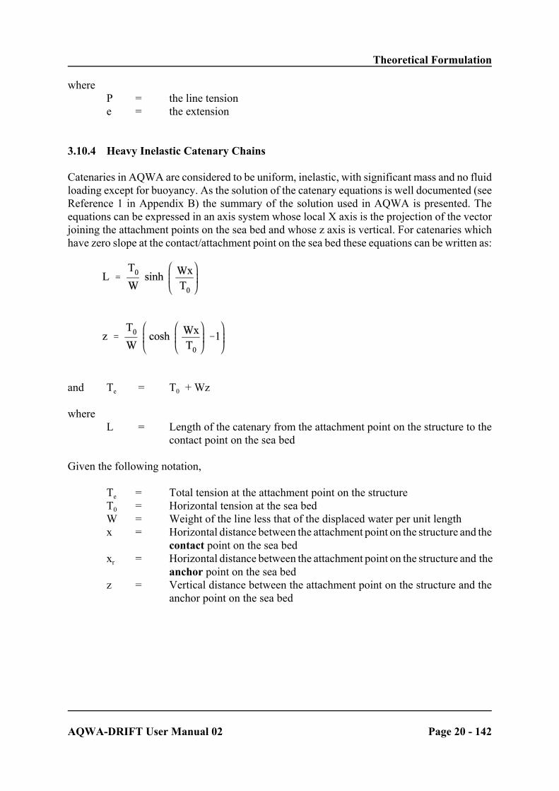
Catenaries in AQWA are considered to be uniform, inelastic, with significant mass and no fluidloading except for buoyancy. As the solution of the catenary equations is well documented (seeReference 1 in Appendix B) the summary of the solution used in AQWA is presented. Theequations can be expressed in an axis system whose local X axis is the projection of the vectorjoining the attachment points on the sea bed and whose z axis is vertical. For catenaries whichhave zero slope at the contact/attachment point on the sea bed these equations can be written as:
and Te = T0 + Wz
whereL = Length of the catenary from the attachment point on the structure to the
contact point on the sea bed
Given the following notation,
Te = Total tension at the attachment point on the structureT0 = Horizontal tension at the sea bedW = Weight of the line less that of the displaced water per unit lengthx = Horizontal distance between the attachment point on the structure and the
contact point on the sea bedxr = Horizontal distance between the attachment point on the structure and the
anchor point on the sea bedz = Vertical distance between the attachment point on the structure and the
anchor point on the sea bed

Theoretical Formulation
AQWA-DRIFT User Manual 02 Page 21 - 142
The stiffness matrix, (K), relating the force to the translational displacements at the attachmentpoint of the structure, is written as:
where
K is rotated about the Z axis until parallel to a reference axis system. The stiffness matrix, K, foreach mooring line is defined at the attachment point on the structure, and must be translated toa common reference point and axis system. In the AQWA suite, the centre of gravity is chosen.This translation, as formulated in Section 3.10.3, is applied to any local stiffness matrix and forceapplied at a point on a structure.

Theoretical Formulation
AQWA-DRIFT User Manual 02 Page 22 - 142
3.10.5 Translation of the Mooring Line Force and Stiffness Matrix
The formulation of a vector translation may be applied directly to a force and displacement inorder to translate the stiffness matrix, K, from the point of definition to the centre of gravity. Itshould be noted however that if the stiffness matrix is defined in a FIXED AXIS SYSTEM,which does not rotate with the structure, an additional stiffness term is required This relates thechange of moment created by a constant force applied at a point when the structure is rotated.
The full 6(6 stiffness matrix (Kg) for each mooring line, relating displacements of the centre ofgravity to the change in forces and moments acting on that structure at the centre of gravity, istherefore given by
where
x,y,z = Coordinates of the attachment point on the structure relative to thecentre of gravity.
Px,Py,Pz = The X, Y and Z components of the tension in the mooring line atthe attachment point on the structure.
Note The term Pm.Tat is NOT symmetric. In general, only a structure in static equilibrium
will have a symmetric stiffness matrix. However this also means that if the mooringforces are in equilibrium with all other conservative forces then the TOTAL stiffnessmatrix will be symmetric.

Theoretical Formulation
AQWA-DRIFT User Manual 02 Page 23 - 142
The force at the centre of gravity (Pg) in terms of the forces at the attachment point (Pa) is givenby:
3.10.6 Stiffness Matrix for a Mooring Line Joining Two Structures
When two structures are attached by a mooring line, this results in a fully-coupled stiffnessmatrix, where the displacement of one structure results in a force on the other. This stiffnessmatrix may be obtained simply by considering that the displacement of the attachment point onone structure is equivalent to a NEGATIVE displacement of the attachment point on the otherstructure. Using the definitions in the previous section the 12(12 stiffness matrix KG is given by:
where
x,y,z = Coordinates of the attachment point on the second structurerelative to its centre of gravity
Px,Py,Pz = The X, Y and Z components of the tension in the mooring line atthe attachment point on the second structure

Theoretical Formulation
AQWA-DRIFT User Manual 02 Page 24 - 142
3.11 WAVE SPECTRA
The method of wave forecasting for irregular seas is achieved within the AQWA suite by thespecification of wave spectra. For further details of spectral forms the reader is referred toAppendix E of the AQWA Reference Manual.
Because of the manner in which the drift force is calculated, it is required that the spectrum bedefined such that the spectral area between adjacent spectral lines is equal. Thus spectral lineswill be close together when the spectral density is large around the spectral peak, and spacedfurther apart when spectral density is low at either end of the spectrum.
The program does this by calculating the spectral density at a very large number of raster pointson the frequency scale, which are equally spaced between the defined spectrum end frequencies.The program uses a default of 5000 raster lines. The raster is then divided into the requirednumber of spectral 'packets' such that the spectral area of each packet is equal. Linearinterpolation is used between the raster points to help define the limits of the packets. A spectralline is then placed at the frequency such that the first moment of area of the spectral energy inthe packet is zero. This is equivalent to defining the spectral line which represents the packet atthe centre of area of the packet.
3.12 STABILITY ANALYSIS
AQWA-DRIFT performs no formal stability analysis. Some physical systems which can bemodelled by AQWA-DRIFT may be inherently statically or dynamically unstable. This may bedetected by careful inspection of the resulting time histories. Note that dynamic instability isdependent on the initial conditions of the simulation. AQWA-LIBRIUM is designed toinvestigate the stability of systems and details are in the AQWA-LIBRIUM manual.
3.13 FREQUENCY DOMAIN SOLUTION
AQWA-DRIFT is a time-domain program for analysis of non-linear systems in irregular waves.Linear systems or linearised systems in irregular waves can be analysed in the frequency-domainby AQWA-FER.

Theoretical Formulation
AQWA-DRIFT User Manual 02 Page 25 - 142
3.14 TIME HISTORY SOLUTION IN IRREGULAR WAVES
3.14.1 Time Integration of Equation of Motion
At each timestep in the simulation, the position and velocity are known since they are predictedin the previous timestep. From these, all the position and velocity dependent forces, i.e. damping,mooring force, total wave force, drift force etc. are calculated. These are then summed to findthe six total forces and moments for each structure (one for each degree of freedom). The totalforce is then equated to the product of the total mass (structural and added) and the rigid bodyaccelerations.
The acceleration at the next timestep can thus be determined. It has been found necessary to usean extremely reliable two-stage predictor-corrector integration scheme to predict the position andvelocity of the structures at the following time increment. The forces are then recomputed withthe new position and velocity and the process is repeated to create, step by step, the time historyof motion.
3.14.2 Motions at Drift Frequency
Large floating structures which are moored at sea, because of their large mass and flexible or'soft' moorings, tend to have natural periods of oscillation in the horizontal degrees of freedomwhich are of the order of minutes. At these periods there is no first order spectral energy so theyare not appreciably excited by first order forces in these degrees of freedom. The structures mayof course have heave, roll or pitch resonances within the range of wave excitation but for themoment we shall consider only the motions in the horizontal freedoms, i.e. surge, sway and yaw.
Section 3.5 explains however that in irregular waves there also exists what are termed secondorder wave forces which oscillate at frequencies which are the difference between pairs of firstorder wave frequencies. These difference frequencies can be very small. Small frequencies implylarge periods which may coincide with the natural period of oscillation of a large floatingstructure. The result of this excitation at periods close to resonance is large amplification factorsin the motions of the structure. These motions are the drift frequency motions.
The equation of motion for the drift frequency motions is:
[ ms + md ] x((t) = Fsv(t) + Fc(t) + Fw(t) + Ft(t) + Fh(t) + Fd(t) (3.14.1)
wherex( = the acceleration vectorms = the structural mass and inertiamd = the added mass and inertia at drift frequency

Theoretical Formulation
AQWA-DRIFT User Manual 02 Page 26 - 142
(3.14.2)
[ Fsv ] = the slowly varying drift force
[ Fc ] = the current forces
[ Fw ] = the wind forces
[ Ft ] = the mooring forces
[ Fh ] = the hydrostatic forces
[Fd] = the damping force
It is assumed that the values of drift added mass/inertia and damping are constant.
3.14.3 Motions at Drift and Wave Frequency
As well as being excited by drift forces, the structure will also be subjected to the first orderwave frequency forces. These forces are added to the list of forces in the drift equation of motionin Section 3.14.2. Since the added mass/inertia and damping are not constant over the wavefrequency range, these forces are modified to allow for this variation. The total wave frequencyforce (i.e. diffraction plus Froude-Krylov) in each degree of freedom is calculated by
wherex(j = -Tj
2 xjx0j = i Tj xji = the imaginary quantity %-1md = the drift added massmj = the added mass at frequency jcd = the drift dampingcj = the damping at frequency jaj = the amplitude of the regular wave componentx = the distance from the origin of the wave system perpendicular to the wave
directionsNj = random phase, frequency jTj = the j th frequencykj = the wave number at frequency jfj = the complex total wave force at frequency jxj = the complex position at frequency j, i.e. the complex response amplitude
operatorx0j = the complex velocity at frequency j

Theoretical Formulation
AQWA-DRIFT User Manual 02 Page 27 - 142
x(j = the complex acceleration at frequency j
and xj = Hj Fj
Hj = (K - Mj Tj2 - i Cj Tj )-1
Mj = ms + ma
wherems = structural mass matrixma = hydrodynamic added mass matrix at frequency jCj = system linear damping matrix at frequency jK = total system stiffness matrixFj = total wave force at frequency j
Equation 3.14.2 shows how a mass difference correction and a damping difference correctionare applied to the total wave force, to correct for the variation of added mass and damping withfrequency. This correction involves a 'best estimate' of the wave frequency response at eachfrequency calculated from the linear equation of motion at that frequency.
The modified total wave force is calculated and added to the sum of all other forces to form theequation motion for drift and wave frequency motions.
[ ms + md ] x((t) = Fsv(t) + Fc(t) + Fw(t) + Ft(t) + Fh(t) + Fwf(t) (3.14.3)
where all terms are as previously defined.
3.14.4 Slow Drift and Wave Frequency Positions
The total motion of the structure can be thought of as comprising a slow drift motion and a fastwave frequency position. These 'slow' and 'wave frequency' positions added together give the'total' position.
When only drift wave forces are present, the structure will execute drift oscillations. This motionis termed the slow motion and its position the SLOW POSITION.
When both drift and wave frequency forces are present, the structure will still perform driftoscillations, but these will be accompanied by wave frequency oscillations about the slowposition. The oscillation about the SLOW position is called the WAVE FREQUENCYPOSITION. The sum of the slow position and the wave frequency position is called the TOTALposition, referred to as simply the POSITION.

Theoretical Formulation
AQWA-DRIFT User Manual 02 Page 28 - 142
(3.14.5)
3.14.5 Response Amplitude Operator Based Position
The wave frequency response of the structure is determined by AQWA-LINE, and is stored inthe form of response amplitude operators at a series of frequencies. A time history of the wavefrequency response can be fabricated by combining the response amplitude operators with thewave spectrum. This is done for each degree of freedom as follows:
whereRe = the real part of the complex expressionxi = the complex response amplitude operator at frequency TiTi = the frequency of a regular wave component in the spectrumki = the wave number of frequency Tixp = the distance from the origin of the wave system perpendicular to the wave
directionai = the amplitude of the regular wave component, frequency iNi = a random phase angle, frequency ix(t) = the instantaneous displacement at time t
and the sum is over all the regular wave components in the discretised spectrum. This is calledthe response amplitude operator based position (RAO BASED POSITION) and is used tocalculate the initial FAST position to minimise transients (see Section 3.14.7).
A similar expression is used to calculate the RAO BASED VELOCITY, using the fact that
x0i = i. Ti .xi
wherex = the complex position at frequency Tix0i = the complex velocity at frequency Ti

Theoretical Formulation
AQWA-DRIFT User Manual 02 Page 29 - 142
3.14.6 Filtering of Slow Position from Total Position
In the case where both drift motion and wave frequency motions exist, the current, and wavedrift forces are applied to the structure in an axis system which follows the SLOW position. Thisis done because the flows take a finite time to develop and cannot follow the rapid oscillationsdue to the wave frequency forces. For example, calculations of current drag, which involve therelative velocity, use the relative velocity between current and SLOW position. The force is thenapplied in the relative direction between current and yaw of the structure. The same applies tothe drift force, but the wind forces are applied using an axis system which follows the totalposition. The slow position is obtained from the total position by filtering the position througha low pass band filter which separates out the slow and fast oscillations. This is achieved byintegrating the following equation at each time step:
x(s + 2.c.Tf .x0s + Tf2 .(xs - xt ) = 0 (3.14.6)
wherex(s,x0s, xs = the filtered slow acceleration, velocity, and positionxt = the total positionTf = the filtering frequencyc = the filter damping
The filter frequency is chosen by the program to eliminate the wave frequency effects. Thedamping is set to 20 percent critical. The SLOW position is filtered out of the TOTAL positionleaving the WAVE FREQUENCY position. It is clear that for simple cases, the RAO BASEDPOSITION will be very similar to the WAVE FREQUENCY position. This can often prove auseful check on the wave frequency position in runs where wave frequency forces are added.
3.14.7 Initial Position and Transients
AQWA-DRIFT solves the second order differential equations of motion for each structure,integrating them to form a time-history. For this, the program requires the initial conditions inorder to begin the integration. Initial conditions are required for the SLOW position and theTOTAL position. Details of how this is done are can be found in Section 4.15D of the AQWAReference Manual. As explained there, for simulations including wave frequency forces, it isusual for the user to allow the program to calculate the initial FAST position, which is added toa defined SLOW position to form the TOTAL POSITION. The FAST or RAO based positionis calculated as described in Section 3.14.5.
This ensures that the TOTAL initial condition contains a FAST component equal to the steadystate solution in response to the wave frequency forces at that instant. By giving the structurean initial SLOW position close to its equilibrium position, transients can be minimised.

Theoretical Formulation
AQWA-DRIFT User Manual 02 Page 30 - 142
3.15 TIME HISTORY SOLUTION IN REGULAR WAVES
Only available within AQWA-NAUT(see AQWA-NAUT manual).
3.16 LIMITATIONS OF THEORETICAL APPLICATIONS
The main theoretical limitations of AQWA-DRIFT should be clearly understood by the user.Since the program uses data calculated by AQWA-LINE, the limitations of the input data mustalso be understood. Refer to AQWA-LINE manual Section 3.15 for details of the assumptionsmade. The AQWA-LINE assumptions which affect the analysis, together with the majorlimitations due to assumptions inherent in AQWA-DRIFT, are listed below:
AQWA-LINE assumptions
1. The theory at present relates to a body or bodies which have zero or small forwardspeed.
2. The wave frequency motions are to first order and hence must be of small amplitude.
3. The fluid domain is assumed ideal and irrotational in the calculations of the added mass,dampings and wave forces.
4. The second order mean wave drift force is calculated using near-field or far-fieldsolution methods. For more information consult the AQWA-LINE manual.
AQWA-DRIFT assumptions
5. The calculation of the slowly varying drift force is accurate only for low frequencies.
6. The drift forces are calculated in the free floating position of the structure and includecomponents due to the first order wave frequency response of the structure. Should thewave frequency response be appreciably altered by the addition of mooring lines notpreviously considered, or any other external influence, then the drift forces will clearlybe in error.
3.17 THE USE OF CONVOLUTION FOR THE EVALUATION OF THERADIATION FORCES IN THE TIME-DOMAIN
By default the AQWA time domain programs, NAUT and DRIFT, assume that the radiationforces can be calculated by using the velocity/acceleration RAOs and added mass/dampingcoefficients at all frequencies to define a set of force RAOs. The radiation force time history canthen be derived from the force RAOs and the wave energy packet. This assumption is only validif the response of the structure at wave frequency is essentially linear, i.e. the structure’s motion

Theoretical Formulation
AQWA-DRIFT User Manual 02 Page 31 - 142
matches RAOs in frequency, amplitude and phase. Since RAOs are calculated for steady stateoscillation under linear forces, the actual structure response, especially when non-linear mooringforce is involved or when the motion has not reached a steady state (i.e transient motion) maydiffer from what is predicted by the RAOs. Consequently the RAO based radiation forcecalculation may no longer be accurate.
In order to address the above problem, users of AQWA have the option of using the ‘convolutionmethod’ (CONV) in the time-domain programs AQWA-DRIFT and AQWA-NAUT. Theconvolution of the added mass and damping from the frequency domain to the time domain isa rigorous treatment of the radiation force which uses the actual structure motion instead ofRAOs. With this method the radiation force is evaluated separately from the other forces anduses the actual velocity/acceleration of the structure rather than the velocity/acceleration basedon the RAOs.
The convolution, as a method of evaluating the radiation forces, can be summarized as follows:
– is more general
– is more accurate for any non linear response
– simplifies the concept of radiation forces
– automatically takes account of non-linear/transient response
– does not require ‘de-coupling’ of low/wave frequency motions.
– automatically calculates interaction between low/wave frequency effects.
With the convolution method, the radiation force is now treated as a totally separate force.Remember that the added mass and damping calculated by AQWA-LINE is only a mechanismfor the calculation of the forces created on a structure by moving that structure in still water insimple harmonic motion at a specific frequency. Strictly speaking, the radiation force in the timedomain can only be calculated if the response of the structure is infinitely small and at freqenciescalculated by AQWA-LINE. In general, the response of a structure will be made up of allfrequencies, which implies that the added mass and damping coefficients must be known at allfrequencies. For the convolution method to be viable, the maximum frequency range practicablemust be calculated by AQWA-LINE. For a tanker this should be from about 0.1 to 1.25radians/sec or 5-60 second periods. This also implies that a minimum of about 800-1000elements (total, all quadrants) is required.
It is also fundamental to understand that the frequency dependent added mass and dampingcoefficients of linear systems are not independent. The added mass from zero to infinity can becalculated totally from the damping by a Fourier transform and inverse (non-symmetric)transform and vice versa. In other words a frequency dependent damping implies the existenceof a frequency dependent added mass and vice versa. If user input of frequency dependent addedmass and damping is accepted in the future for convolution then it will be required to obey thiscriterion.

Theoretical Formulation
AQWA-DRIFT User Manual 02 Page 32 - 142
The convolution method as implemented in AQWA-DRIFT and NAUT has 4 distinct stages:
1. Extrapolation of added mass/damping from zero to ‘infinity’.
2. The calculation of the time history convolution integral function (CIF).
3. Interpolation of the CIF at an integral number of time steps
4. Calculation of the radiation force at any time by integrating the CIF.
Steps 1 to 3 are performed for each analysis before starting the time history simulation.
The convolution method, as a method of evaluating the radiation as well as the diffraction forces,appears extensively in the literature. Users wishing to study the convolution method in moredetail may refer to ref. [6] and [7].

Modelling Techniques
AQWA-DRIFT User Manual 02 Page 33 - 142
CHAPTER 4 - MODELLING TECHNIQUES
This chapter relates the theory in the previous section to the general form of the input datarequired for the AQWA suite. The sections are closely associated with the sections in theprogram input format. All modelling techniques related to the calculations withinAQWA-DRIFT are presented. This may produce duplication in the user manuals where thecalculations are performed by other programs in the suite. Other modelling techniques which areindirectly related are included to preserve subject integrity; these are indicated accordingly.
Where modelling techniques are only associated with other programs in the AQWA suite, theinformation may be found in the appropriate sections of the respective manuals (the sectionnumbers below correspond to those in the other manuals as a convenient cross reference).

Modelling Techniques
AQWA-DRIFT User Manual 02 Page 34 - 142
4.1 INTRODUCTION
When using AQWA-DRIFT we do not require a description of the full structure surface. Insteadthe properties of the structure are described numerically. The hydrostatic properties are definedby a stiffness matrix and the hydrodynamic properties are defined by hydrodynamic loadingcoefficients and wave forces, which are the RESULTS of calculations by programs likeAQWA-LINE, which use models involving geometric surface definitions.
When AQWA-LINE is run, all these parameters are transferred automatically to backing filesfor future use with other AQWA programs.

Modelling Techniques
AQWA-DRIFT User Manual 02 Page 35 - 142
4.2 MODELLING REQUIREMENTS FOR AQWA-DRIFT
4.2.1 When Used as an Independent Program
AQWA-DRIFT requires the following categories of modelling information:
1. Body mass and inertia characteristics.
2. Wave hydrodynamic and hydrostatic description.
3. Wind and current force coefficient description.
4. Description of mooring configuration.
5. Analysis environment description.
6. Time integration parameters.
These categories will be described in the following sections:
4.2.2 Following an AQWA-LINE Run
After an AQWA-LINE run or a series of runs has been completed, then it may be required toutilise the results in an AQWA-DRIFT analysis. AQWA-LINE automatically produces aHYDRODYNAMICS DATABASE file and a RESTART file. These contain all the informationrequired by AQWA-DRIFT, concerning the structure's mass and inertia properties, thehydrostatic properties and the wave hydrodynamic properties (in the form of a description of theadded mass, damping and wave forces, at a series of regular wave frequencies).This informationcorresponds to categories 1 and 2 of Section 4.2.1 which, if requested, is automaticallytransferred to the AQWA-DRIFT run, the remaining information being provided by auser-prepared data file.

Modelling Techniques
AQWA-DRIFT User Manual 02 Page 36 - 142
4.3 DEFINITION OF STRUCTURE AND POSITION
Full details may be found in the Aqwa Reference Manual.
4.3.1 Axis Systems
AQWA-DRIFT uses several axis systems for different purposes.
1. Fixed Reference Axes (FRA)
The OXY plane of the FRA lies on the free surface and OZ points vertically upwards.
2. Local System Axes (LSA)
The LSA axis are fixed to the vessel with their origin at the centre of gravity. Theycoincide with the FRA when the vessel is in its definition position.
3. Slow Axis System (SLA)
The slow axis system is similar to the LSA in that its origin is located at the centre ofgravity, but differs in that it follows only the slow drift motion of the structure.
4.3.2 Conventions
The AQWA suite employs a common sign convention with the axes defined in the previoussection.
Translations of a body in the X, Y and Z direction are termed SURGE, SWAY and HEAVE andare positive in the positive direction of their respective axes. Rotations about the X, Y and Z axes(of the FRA) are termed ROLL, PITCH and YAW. The positive sense of these is determined bythe right hand screw rule.

Modelling Techniques
AQWA-DRIFT User Manual 02 Page 37 - 142
4.3.3 The Structural Definition and Analysis Position
In the description of the body geometry and mass distribution, the user may define the structurein any position. There are, however, three important considerations when choosing the positionin which to define the structure.
e.g. If the structure is a ship or barge, conventional terminology for motion along, androtation about the longitudinal axis is SURGE and ROLL. However, if the longitudinalaxis is defined parallel to the FRA Y-axis then rotational motion about this axis will betermed PITCH, and translational motion along this axis SWAY. Thus, conventionalbody surge and roll will be termed sway and pitch by the program.
For other structures, e.g. semi-submersibles, this may not be so relevant. The user must take duenote of the terms associated with the motions about the axes and is recommended to define allship/barge shaped structures with the longitudinal axis parallel to the FRA X-axis.

Modelling Techniques
AQWA-DRIFT User Manual 02 Page 38 - 142
4.4 STRUCTURE GEOMETRY AND MASS DISTRIBUTION
When AQWA-DRIFT is used following an AQWA-LINE run (the normal mode of analysisprocedure) the structure geometry and mass distribution are transferred automatically from thebacking files produced by AQWA-LINE. This section therefore describes the modelling of thestructure geometry and mass distribution when AQWA-DRIFT is used independently (see theAQWA- LINE and AQWA-LIBRIUM manuals when this is not the case).
Note that a hydrostatic or hydrodynamic model as such is not required (see Section 4.2.1), onlythe hydrostatic stiffness matrix (see Section 3.1.3) and hydrodynamic loading coefficients (seeSection 3.3).
4.4.1 Coordinates
Any point on the structure in the modelling process is achieved by referring to the X, Y and Zcoordinate of a point in the FRA which is termed a NODE. The model of structure geometry andmass distribution consists of a specification of one or more elements (see also Sections 4.1,4.4.2) whose position is that of a node. Each node has a NODE NUMBER, which is chosen bythe user to be associated with each coordinate point. Nodes do not contribute themselves to themodel but may be thought of as a table of numbers and associated coordinate points which otherparts of the model refer to.
Although several coordinates must be defined if several elements are used to define thegeometry/mass distribution, normally a single point mass is used, which means that only a singlenode is defined at the centre of gravity of the structure.
Note that nodes are also used to define the position of other points, not necessarily on thestructure, e.g. the attachment points at each end of a mooring line.
4.4.2 Elements and Element Properties
As stated in the previous section, the structural geometry and mass distribution of the model forAQWA-DRIFT, used independently of AQWA-LINE, is achieved by specifying one or moreelements, which in total describe the whole structure. The only elements required are POINTMASS elements. A point mass has a position, a value of mass, (e.g. 12 tonnes), and a massinertia. These in turn are defined by the specification of
- a node number- a material number- a geometric group number
The node number (described in the previous section) and the material and geometric groupnumber, are numbers which refer to a table of values of coordinates, masses and structuralinertias respectively. Once defined in the table, the numbers may be referred to by any numberof elements.

Modelling Techniques
AQWA-DRIFT User Manual 02 Page 39 - 142
4.5 MORISON ELEMENTS
There are three Morison elements available within AQWA-DRIFT and AQWA-NAUT, namely:
! Tube element (TUBE)! Slender Tube element (STUB)! Disc element (DISC)
Tube elements are defined by specifying end nodes, diameter, wall thickness and endcut lengths(over which the forces are ignored). Each tube element may have a different drag and addedmass coefficient associated with it. Drag coefficients can be defined as functions of ReynoldsNumber.
Full consideration is given to the variation of local fluid motion over the tube length and topartial submersion of members.
Morison drag and added mass are evaluated on all submerged or partially submerged tubes but,if the user wishes to suppress these calculations, the drag and added mass coefficients on any orall tubes of a given structure may be set to zero.
Slender tube (STUB) elements differ from TUBE elements in the following respects:
1. STUB elements permit tubes of non-circular cross section to be modelled, by allowingthe tube properties (diameter, drag coefficient, added mass coefficient) to be specifiedin two directions at right angles.
2. Longer lengths of tube can be input, as the program automatically subdivides STUBelements into sections of shorter length for integration purposes.
3. An improved (second order) version of Morisons equation is used to calculate the dragand inertia forces on STUB elements. This is particularly useful in the study of droppedobjects.
4. STUB elements should, however, only be employed if the (mean) diameter is smallcompared with the length.
A DISC element (DISC) has no thickness and no mass (users can define a PMAS and attach itto a disc if necessary), but has drag coefficient and added mass coefficient in its normaldirection. Therefore, a DISC does not have Froude-Krylov and hydrostatic force. A DISCelement has only a drag force and an added mass force.
4.5.1 Reynolds Number Dependent Drag Coefficients
Reynolds number effects on drag can be important at model scale. Drag coefficients are normallyconsidered constant (as is often the case at full scale, i.e. large Reynolds numbers). However,

Modelling Techniques
AQWA-DRIFT User Manual 02 Page 40 - 142
experimental evidence shows that the Reynolds number is not just a simple function of thevelocity and diameter for cylinders with arbitrary orientation to the direction of the fluid flow.Considerable improvement in agreement with model tests can be obtained by using a scale factorto obtain a local Reynolds Number and interpolating from classical experimental results,
whereLocal Reynolds Number = (U*D/<) / (scale factor) U = local fluid velocity transverse to the axis of the
tube D = tube diameter< = kinematic viscosity of water
from which drag coefficients can be interpolated from the Wieselberg graph of drag coefficientversus Reynolds number for a smooth cylinder.
Alternatively, a general multiplying factor for drag can be used.
4.5.2 Morison Forces For AQWA-DRIFT with no Wave Frequency Motions
When the wave frequency motions are omitted in an AQWA-DRIFT analysis (i.e. when it hasbeen specified that only drift motions are required), the user has effectively requested that thewave frequency forces on the Morison elements should be omitted, i.e. the forces are to becalculated using only the low frequency motions of structures (including riser and space framestructures).
Although the inertia forces do not usually alter the motions of the main vessel, the drag forcesmay be significant in contributing to a lightly damped vessel (e.g. in surge).
The user should therefore estimate the additional overall drag-type loading (for input into Deck10 as 'Hull Drag') or estimate the equivalent linear damping (for input into Deck 7) for the wavespectrum used using the R.M.S wave velocity and Morisons equations for all the Morisonelements. If the user is in doubt as to the accuracy of the results, he should run first with noadditional damping, and then with the drag/damping described above, to ascertain the sensitivityof the overall motion of the vessel to the forces on the Morison elements.

Modelling Techniques
AQWA-DRIFT User Manual 02 Page 41 - 142
4.6 STATIC ENVIRONMENT
4.6.1 Global Environmental Parameters
The global or static environmental parameters are those which remain constant or staticthroughout an analysis and comprise the following:
Acceleration due to Gravity: Used to calculate all forces and variousdimensionless variables throughout theprogram suite.
Density of Water: Used to calculate fluid forces and variousdimensionless variables throughout the programsuite
Water Depth: Used in AQWA-DRIFT, through the wavenumber, to calculate phase relationshipsfor various parameters.

Modelling Techniques
AQWA-DRIFT User Manual 02 Page 42 - 142
4.7 LINEAR STIFFNESS
4.7.1 Hydrostatic Stiffness
The hydrostatic stiffness matrix is calculated in AQWA-LINE and then transferred automaticallyvia backing file to the other programs in the suite when they are used as post-processors toAQWA-LINE. More details may therefore be found in the AQWA-LINE manual in Section4.7.1.
When AQWA-DRIFT is used independently, the linear hydrostatic stiffness matrix is requiredas input data. Note that, although this matrix is termed 'linear hydrostatic', a matrix may be inputwhich includes other linear stiffness terms. However, the user is advised to consider other linearstiffness terms as ADDITIONAL stiffness to be modelled separately as described in thefollowing section.
4.7.2 Additional Linear Stiffness
The additional linear stiffness is so called to distinguish between the linear hydrostatic stiffnesscalculated by AQWA-LINE (or from any other source) and linear stiffness terms from any othermechanism or for parametric studies. As this stiffness matrix is transferred automatically frombacking file when AQWA-DRIFT is used as a post-processor the following notes refer toAQWA-DRIFT when used as an independent program.
Although all terms in the additional linear stiffness can be included in the hydrostatic stiffnessmatrix, the user is advised to model the two separately. The most common reasons for anadditional stiffness model are:
- modelling facilities for a particular mechanism are not available in the AQWA suite
- the hydrostatic stiffness matrix is incomplete
- the user wishes to investigate the sensitivity of the analysis to changes in the linearstiffness matrix.
In practice, only in unusual applications will the user find it necessary to consider the modellingof additional linear stiffness.

Modelling Techniques
AQWA-DRIFT User Manual 02 Page 43 - 142
4.8 WAVE FREQUENCIES AND DIRECTIONS
The wave frequencies and directions are those at which the wave loading, current and windcoefficients are defined and, as they are transferred automatically from backing file whenAQWA-DRIFT is used as a post-processor, the following notes refer to AQWA-DRIFT whenused as an independent program.
These coefficients, which are required as input data (further details may be found in thefollowing sections) are dependent on frequency and/or direction. A range of frequencies anddirections is therefore required as input data, which are those at which the coefficients aredefined.
There are only two criteria for the choice of values of the frequency and direction which may besummarised as follows:
1. The extreme values must be chosen to adequately define the coefficients at thosefrequencies where wave energy in the spectra chosen (see Section 4.14) is significant,and at ALL possible directions of the subsequent response analysis. If geometricsymmetry has been specified (see Section 4.3.3 para 2.) only those directions for thedefined quadrants are required.
2. Sufficient values are required to adequately describe the variation of these coefficientsdefined.
Clearly, if either of these criteria is violated, approximate results will be obtained. Wherepossible, the program will indicate this accordingly. However, this should not be relied on asanticipation of the intentions of the user is not usually possible.

Modelling Techniques
AQWA-DRIFT User Manual 02 Page 44 - 142
4.9 WAVE LOADING COEFFICIENTS
The wave loading coefficients are calculated by AQWA-LINE and then transferred automaticallyfrom backing file when AQWA-DRIFT is used as a post-processor. Thus the following notesrefer to AQWA-DRIFT when used as an independent program. This information falls into fivecategories. These are:
1. Frequencies and directions at which the regular wave loading has been calculated
2. Added mass and inertia matrices at each frequency
3. Damping coefficient matrices at each frequency
4. Diffraction and Froude Krylov wave forces at each frequency and direction
5. Drift forces at each frequency and direction
It is important that the wave frequency parameters are defined over the range of expected waveexcitation frequencies, and that the direction- dependent parameters are defined over theexpected RELATIVE angle of incidence.
For wave frequency motion, the added mass and damping matrices are required for the range offrequencies. The diffraction and Froude Krylov forces are required for the range of frequenciesAND for the range of directions. AQWA-DRIFT combines the diffraction and Froude-Krylovforces from AQWA-LINE into a resultant total wave force. If the forces are being inputmanually, the user can input wave forces as either Froude Krylov or diffraction, since theprogram does not differentiate between the two.
For drift frequency motion, a single added mass and damping matrix are required. Theseapproximate the values of added mass and damping for low frequency motions, which normallyinclude those at drift frequency. The drift forces are calculated by AQWA-DRIFT from theregular wave drift force coefficients, which are defined for the range of frequencies anddirections. The added mass varies with frequency of oscillation. As the frequency of oscillationtends to zero, the added mass tends to an asymptotic value. This asymptotic value is a goodapproximation to the drift added mass. In practice, the added mass of a typically large floatingstructure, e.g. a 100,000 tonne DWT tanker, is close to its asymptotic value at periods of 25 sec.The longest period wave frequency run should be chosen to provide a suitable value of driftadded mass.

Modelling Techniques
AQWA-DRIFT User Manual 02 Page 45 - 142
4.10 WIND AND CURRENT LOADING COEFFICIENTS
The wind and current loading coefficients are required to model the forces and moments on thestructure due to wind and current. These forces are proportional to the square of the relativevelocity.
For a simple box shape or similar bluff bodies, these coefficient may be reasonably wellapproximated by consideration of projected frontal areas and a suitable drag coefficient. Forhydrodynamic geometries, e.g. a tanker, net lift forces may also be important. O.C.I.M.F. haspublished results of model tests on various tankers (see Reference 4).
4.11 THRUSTER FORCES
Thruster forces can be applied on any point of the structure in any direction. Two trusters canproduce a moment by acting in parallel directions but not through the same point.
4.12 CONSTRAINTS OF STRUCTURE MOTIONS
The facility of de-activating degrees of freedom is most often used when in the simulation of thedrift motion of a structure. Here only the surge, sway and yaw degrees of freedom are of interest,and it is therefore not required that the roll, pitch and heave degrees of freedom be integrated.The position of these non-active freedoms will stay constant and equal to the initial defined valuethroughout the simulation. It is therefore important to specify these correctly.
Great care must be exercised if the degrees of freedom are de-activated in a structure which isarticulated either to another structure or to a fixed point. It is recommended that this should notbe done.

Modelling Techniques
AQWA-DRIFT User Manual 02 Page 46 - 142
4.13 STRUCTURAL ARTICULATIONS
4.13.1 Articulations
Structures in an AQWA-DRIFT analysis can be freely floating, moored or connected to otherstructures by points of articulation. There are four different types of articulation available. Theseare as follows:
0 Ball and Socket Free to rotate in all freedoms
1 Universal Free to rotate in two freedoms transmitting a moment inthe third freedom at right angles to the first two
2 Hinged Transmitting a moment in two freedoms and free to rotatein the third freedom at right angles the first two
3 Locked Transmitting a moment in all three freedoms and not freeto rotate at all.
4.13.2 Constraints
A constraint can be applied to any degree of freedom. This has the effect of stopping thecalculation of forces or moments, and stopping motion in the specified constrained degrees offreedom.

Modelling Techniques
AQWA-DRIFT User Manual 02 Page 47 - 142
4.14 WAVE SPECTRA, WIND AND CURRENT SPECIFICATION
The user may specify only one spectrum, wind and current speed and their associated directions.For the majority of applications, specification is quite straightforward and no knowledge of theway in which the spectra are used in any program is required. The two rules for specification ofthe spectrum are as follows:
1. The value of the spectral ordinate at the beginning and end of the frequency rangeshould be small. If the values are not small, only part of the spectrum has effectivelybeen specified.
2. The frequency defining the lower range of the spectrum must be smaller than thelowest frequency specified in Deck 6, as the frequency at the lower end of the rangeis used as both an upper limit to the drift frequencies and a lower limit to the wavefrequencies.

Modelling Techniques
AQWA-DRIFT User Manual 02 Page 48 - 142
4.15 MOORING LINES
4.15.1 Linear/Non-Linear Elastic Hawsers
The line properties are specified by their unstretched lengths, ends nodes on respective bodiesand their load/extension characteristics. For linear hawsers, the line stiffness (load per unitextension) is required. For non-linear hawsers, the program permits up to a fifth orderpolynomial approximation of the elastic property of the following form:
P(e) = a1 e + a2 e2 + a3 e3 + a4 e4 + a5 e5 (4.15.1)
where P = the line tension e = the extension
The use of a higher order polynomial than necessary could lead to erroneous negative stiffnesswhile a lower order fit could be perfectly adequate (see Figure 4.2). It is always useful to checkthe polynomial fit prior to its use as input data. Note that the term a1 is usually a goodapproximation to the linear stiffness for small extensions.
Figure 4.2 - Load/Extension Characteristics
Modelling Techniques
AQWA-DRIFT User Manual 02 Page 49 - 142
4.15.2 Constant Tension Winch Line
The winch line is characterised by its constant tension, attachment points an 'unstretched length'.The attachment points are specified as nodes and determine the direction of the constant tension.The 'unstretched length' allows the line to go slack when the distance between the end points isless than it. If the user requires constant tension at all times, a zero unstretched length may beinput.
4.15.3 ‘Constant Force’ Line
The program allows the user to input a force of constant magnitude and direction. The force isalways assumed to act at the centre of gravity of the body. The direction of the force is specifieda node on the body and a second node chosen such that the force vector is directed from node1 to node 2. Once the direction is defined, the program maintains the magnitude and directiondespite movement of the body. This facility can be used to input environmental forces wheredetails of the forces (e.g. wind coefficients) are not available.
4.15.4 Catenary line
The catenary model admits uniform, inelastic, heavy catenary lines. Current drag on the lineitself is ignored. The line is specified by the end nodes, length, weight in air per unit length andequivalent cross sectional area. The equivalent cross sectional area is numerically equal to thevolume of water displaced by a unit length of the chain.
The user may specify maximum and minimum tensions in the line and maximum tension at theanchor. Default values are provided by the program. For length based calculations, the programwill adjust the line length if the tension turns out to be outside the range specified (or the defaultvalues). If the user wishes to keep constant line length irrespective of the tension, a very largevalue of maximum allowable tension may be input. In all cases, adequate warning messages willbe signalled.
The program evaluates the line tension and stiffness according to close form solution of thecatenary equations. The program allows the line to lift off the sea bed (i.e. the tangent to the lineat the anchor has non-zero slope) up to the point where the line tension exceeds a userspecified/default maximum.
Care must be exercised in the description of the catenary line such that the line is not lyinghorizontally and the length is sufficient to allow the expected range of movement of its ends.Although the program caters for cases where the catenary line lifts off the sea bed, in practice,most catenary chains are expected to function with a significant length of the line on the sea bed.
The following expression may help the user to check in advance if the catenary is likely to liftoff from the sea bed. Just at lift off, T, the tension in the line is approximately related to s, theline length by the simple expression
T/W = (s2 + z2 )/2z (4.15.2)

Modelling Techniques
AQWA-DRIFT User Manual 02 Page 50 - 142
whereW = the 'weight in water' per unit length of the chainz = the vertical distance between the anchor point and the attachment point
on the body
By specifying T as given by equation (4.15.2) as the maximum tension, the user can ensure thatthe line does not 'lift off'.
4.15.5 Steel Wire Cables
The Steel Wire (SWIR) facility allows modelling of the non-linear properties of a new steel wirerope. Although the SWIR cable is classified as a non-linear cable it is possible to model steelwire using linear (LINE) or non-linear (NLIN) lines.
4.15.6 Intermediate Buoys and Clump Weights
The Buoy card (BUOY) defines the properties of intermediate buoys and clump weights.Intermediate buoys cannot be used between structures but only between a structure and the seabed.
4.15.7 The Pulley Card (PULY)
The PULY facility allows the use of a pulley positioned on a line. A maximum of 2 pulleys isallowed for each pulley set. A PULY card must be proceeded by a LINE card.
4.15.8 The Drum Winch (LNDW)
The LNDW card is used to model a winch or drum winch which winds in or pays out a linearelastic line starting at a user specified time.
4.15.9 Fenders (FEND)
Fixed and floating fenders are available in AQWA. A fixed fender is graphically shown as asphere in the AGS, or if the axis is defined, a cone whose axis is normal to structure plane towhich it is fixed. A floating fender will be shown as a short cylinder. Emphasis has been puton the “realistic” graphical representation of the fender distortion. Fixed and floating fendersin AQWA can be modelled together with conventional mooring lines.

Modelling Techniques
AQWA-DRIFT User Manual 02 Page 51 - 142
4.16 ITERATION PARAMETERS FOR SOLUTION OF EQUILIBRIUM(AQWA-LIBRIUM ONLY)
Not applicable to AQWA-DRIFT (see AQWA-LIBRIUM manual).

Modelling Techniques
AQWA-DRIFT User Manual 02 Page 52 - 142
4.17 TIME HISTORY INTEGRATION IN IRREGULAR WAVES
4.17.1 Timestep for Simulation
The timestep for a simulation should be chosen to be a small fraction of the period of variationof the most rapidly varying force or response. A different timestep is applicable if investigatingonly drift motions, as opposed to drift and wave frequency motions.
Drift motions
In this case only drift motion are being integrated and the timestep should be about one twentiethof the smallest natural period of drift oscillation. A 5 to 10 second timestep is usual for a typicaloffshore structure.
Drift and wave frequency motions
A suitable timestep in this case will be much shorter, since the response to wave frequency forcesis being investigated. A timestep of 0.5 seconds is typical.
Once a timestep has been selected, the program outputs an indication of the expected errors usingthe chosen timestep. This is explained in Section 7.6 in the description of the output. Theprogram also outputs the error at each timestep in each degree of freedom which is related to thechosen timestep. These errors can always be reduced by shortening the timestep.
4.17.2 Simulation Length and Accuracy Limits
For the time history of motion in an irregular sea to be representative of the structure's motioncharacteristics in that sea, the time history has to be of sufficient length to allow averaging ofmaximum and minimum response. Motions simulated over a finite length of time contain somestatistical error because the sample may, by chance, contain an unrepresentative number of largeor small oscillations. Reference 5 explains that the variance of the mean square value of the slowdrift position can be calculated assuming linear mooring stiffness and linear damping. This canprovide a useful guide to the expected errors in statistical properties derived from a finite lengthsimulation.
The variance of the mean square value can be calculated form the following:
(4.17.1)
whereF2 = the true mean squared valueD(t) = the auto-correlation function of the process T = the length of the simulation or process
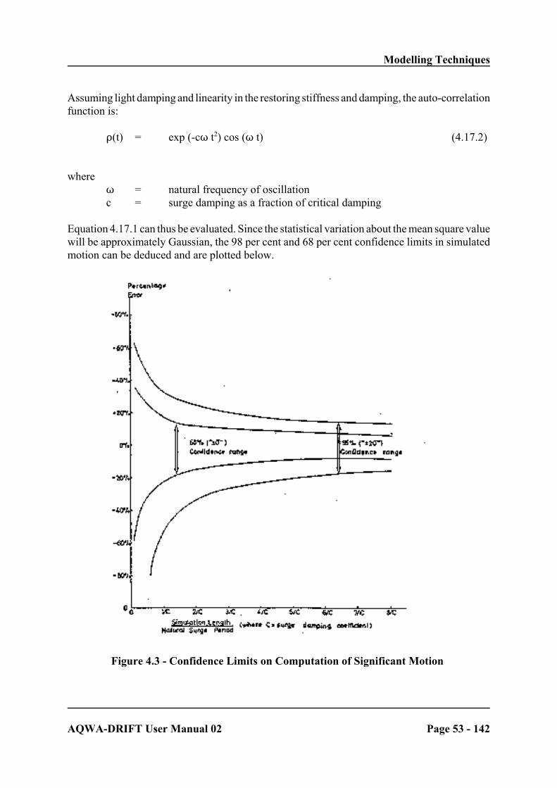
Modelling Techniques
AQWA-DRIFT User Manual 02 Page 53 - 142
Assuming light damping and linearity in the restoring stiffness and damping, the auto-correlationfunction is:
D(t) = exp (-cT t2) cos (T t) (4.17.2)
whereT = natural frequency of oscillationc = surge damping as a fraction of critical damping
Equation 4.17.1 can thus be evaluated. Since the statistical variation about the mean square valuewill be approximately Gaussian, the 98 per cent and 68 per cent confidence limits in simulatedmotion can be deduced and are plotted below.
Figure 4.3 - Confidence Limits on Computation of Significant Motion

Modelling Techniques
AQWA-DRIFT User Manual 02 Page 54 - 142
The graph shows that for a system with 10 percent damping, the length of simulation must beat least 40 times the structures natural period to achieve an estimate of the significant motioncorrect to +/- 20 per cent.
4.17.3 Initial Conditions and Start Time
It is important that the simulation should have as small an initial transient at the start as possible,especially if the user requires accurate statistics of the simulations; transients at the start willinvalidate the statistics of the run. It is usual when performing a drift motion simulation toposition the structure close to the equilibrium position of the structure under the influence ofsteady forces.
The user may then wish to add in the wave forces over a short segment of the drift run startingjust before a peak drift response. This would, for example, indicate how much the wavefrequency effects will modify the peak motions and tensions in mooring lines. To do this, theuser must pick off the slow position and velocity at some appropriate time in the drift run andthen perform another simulation with these slow positions and velocities as the startingconditions. It is very important for the user to remember to give this second simulation a startingtime equal to that at which the slow position and velocity occurred, so that the second simulationhas exactly the same wave force time history as the first.

Modelling Techniques
AQWA-DRIFT User Manual 02 Page 55 - 142
4.18 TIME HISTORY INTEGRATION IN REGULAR WAVES(AQWA-NAUT ONLY)
Not applicable to AQWA-DRIFT (see AQWA-NAUT manual).
4.19 SPECIFICATION OF OUTPUT REQUIREMENTS
See options list in Appendix A.

Analysis Procedure
AQWA-DRIFT User Manual 02 Page 56 - 142
CHAPTER 5 - ANALYSIS PROCEDURE
This chapter assumes that the user is familiar with the theory of the analysis and how to modelthe structure in its environment. It deals with the method of analysis associated with running theprogram and links the modelling information in the previous chapter with the stages of analysisnecessary to solve a given type of problem. This involves classification of the types of problem,and details of the program runs and stages within each program run together with their associatedoptions.

Analysis Procedure
AQWA-DRIFT User Manual 02 Page 57 - 142
5.1 TYPES OF ANALYSIS
There are several different common types of analysis that the program has been designed toperform. These are the same whether used independently, or as a post-processor toAQWA-LINE, and are as follows
1. Investigation of transient response of coupled moored structures 2. Simulation of drift motions of coupled moored structures 3. Simulation of drift and wave frequency motions of coupled moored structures
In each of these analyses, any chosen variables can be analysed statistically and plotted ifrequired. The different types of analyses and the results that are produced are mainly controlledby program options.
5.2 RESTART STAGES
All programs in the AQWA suite have the facility of running one or more stages of the analysisseparately. These stages are referred to in the documentation as RESTART STAGES (seeChapter 2 of the AQWA Reference Manual).
Use of the restart process thus implies that information is available on a backing file from aprevious program run and not via the normal card image file. This process is also used to transferinformation from one program to another program in the AQWA suite.
These stages are as follows:
Stage 1 - Geometric Definition and Static Environment Stage 2 - Input of the Diffraction/Radiation Analysis Parameters Stage 3 - The Diffraction/Radiation AnalysisStage 4 - Input of the Analysis EnvironmentStage 5 - Motion AnalysisStage 6 - Graphical Display of Model and Results
Note that the graphics will allow visualisation of the geometric model and parameters at anypoint in the analysis, e.g. Stages 2 to 5 are not required to visualise the data input in Stage 1.This only applies to the graphics, as all other programs must progress from one stage to anotherwith NO stages omitted. As Stage 3 has no direct calculations in programs other thanAQWA-LINE, the programs will 'correct' a request to finish at Stage 2 to one to finish at Stage3. This remains transparent and requires no action by the user.

Analysis Procedure
AQWA-DRIFT User Manual 02 Page 58 - 142
5.3 STAGES OF ANALYSIS
An analysis using AQWA-DRIFT independently uses the items 1 to 7 of the following. If theprogram is being used as a post processor to AQWA-LINE then this information is automaticallytransferred from AQWA-LINE to AQWA-DRIFT.
1. Select a consistent set of units.
2. Identify the geometric and material data for the body or bodies.
3. List all relevant co-ordinates.
4. Specify one or more point masses to represent the mass and mass inertia of each of thestructures.
5. Specify the hydrostatic stiffness together with the position at which the gravity andhydrostatic forces together are zero.
6. Specify the wave diffraction/radiation coefficients and the frequencies and directionsat which they are defined for each structure.
7. Specify the wave drift coefficients if drift motions are significant for each structure.
The following items 8 to 14 are required for AQWA-DRIFT used independently or as apost-processor to AQWA-LINE.
8 Determine mooring line properties.
9. Prepare coefficients for wind and current drag for each structure.
10. Specify the wave damping and added mass applicable to low frequency motion for eachstructure.
11. Specify initial positions for each spectrum and details of the simulation length andtimestep length.
12. Create a data file as described in Chapter 6.
13. Perform a DATA run (i.e. with the DATA option switched on) which will providepreliminary checks on the card image data file.
14. After a successful DATA run, select mode of analysis on the first card of the card imageinput data (drift motion or drift plus wave frequency) and re-run with the restart option.

Analysis Procedure
AQWA-DRIFT User Manual 02 Page 59 - 142
The usual analysis procedure is to first look at the drift motions of a structure in a driftsimulation.
The relative importance of wave frequency effects can then be determined by performing a driftplus wave frequency motion simulation. It is usual to perform this wave frequency simulationstarting at some point just before the maximum drift response to see how the peak response isaggravated or reduced by the wave frequency effects. From the output listing of the drift run, itis possible to pick off the structure's position and velocity at some time just before the peak driftmotion and use these as the initial conditions for the wave frequency simulation.
Data Preparation
AQWA-DRIFT User Manual 02 Page 60 - 142
CHAPTER 6 - DATA REQUIREMENT AND PREPARATION
This chapter describes the form in which data is expected by the program and it is not intendedas a detailed list of the data requirements and general format for each type of analysis that maybe performed when running AQWA-DRIFT. The detailed format may be found in the AQWAReference Manual. The data file is constructed by a series of data decks.
A summary of all possible data that may be input is listed together with a summary for variousforms of analysis. In this latter case a TYPICAL input data summary is used where the moreunusual facilities have been omitted.
Most data requirements listed are optional unless specified otherwise and if not input theprogram defaults are used. These defaults may be found, together with the detailed formatdescription, in the AQWA Reference Manual.

Data Preparation
AQWA-DRIFT User Manual 02 Page 61 - 142
6.0 ADMINISTRATION CONTROL - DECK 0 - PRELIMINARY DECK
This deck is always required when performing AQWA program analysis runs. The informationinput relates directly to the administration of the job being done and the control of the AQWAprogram being used.
Program control has the following functions:
- identification of the program to be used within the AQWA suite - the type of program analysis to be performed (i.e. if choice exists) - the analysis stage to be performed (i.e. restart stages)
Administration of the analysis being performed is as follows
- user title identification given to the analysis- choice of output required from program run (i.e. program options)
The above information is input to the program through the following cards contained in Deck0.
JOB Card - This contains information stating the program to be used, the typeof program analysis to be undertaken and the user identifier forthe run in question.
TITLE Card - This lets the user prescribe a title for the run.
OPTIONS Card - Various program options are available within the AQWA suitewhich are common to all programs while others are for use withspecific programs. The options within AQWA-DRIFT control thetype of output required from the program and the restart stages ofanalysis to be performed (see Appendix A).
RESTART Card - If the restart option is used, then the start and finish stages of theanalysis must be prescribed via the restart card.
For complete details of the above card formats see the AQWA Reference Manual. For a list ofoptions for use within AQWA-DRIFT, see Appendix A.

Data Preparation
AQWA-DRIFT User Manual 02 Page 62 - 142
One option commonly used is the DATA option and it is worth noting its purpose. The DATAoption performs Stages 1 to 4 of an AQWA-DRIFT analysis. This means that all informationrelating to the analysis is read in allowing all data checking to be performed. After the user issatisfied with the acceptance of data then the analysis can be undertaken by restarting theprogram at Stage 5 to perform the analysis itself.

Data Preparation
AQWA-DRIFT User Manual 02 Page 63 - 142
6.1 STAGE 1 - DECKS 1 TO 5 - GEOMETRIC DEFINITION AND STATIC ENVIRONMENT
Input for Stage 1 of the analysis is only necessary if the restart stage at which the analysis beginsis 1 (see Chapter 5). If the restart stage is greater than 1, there is NO INPUT for Stage 1 of theanalysis.
6.1.1 Description Summary of Physical Parameters Input
The data input in these decks relates to the description of each structure and the environmentwhich normally remains unchanged throughout the analysis. This includes any point referencedon or surrounding the structure, the mass inertia, hydrostatic and hydrodynamic model and the(constant) water depth, i.e.
- the coordinates of any point on the structure or its surrounding referenced by any otherdeck
- point mass element description of the mass distribution - a table of masses associated with each point mass- a table of inertias associated with each point mass - the depth and density of the water and acceleration due to gravity
The data requirements of each program are not the same and may be also dependent on the typeof analysis performed. These requirements are listed in detail in the later sections of this chapter.
6.1.2 Description of General Format
The input format these decks is designed to provide checking on the data for the average user,and outputs a suitable message to inform the user if the instructions for data preparation havebeen misinterpreted or are unusual. When running with a DATA option for the first time it isrecommended that the PRCE (PRint Card Echo) option is used (see Appendix A), as the datainput in these decks (1-5) is not echoed automatically. The user may then check the results beforeproceeding to Stage 2 of the analysis.

Data Preparation
AQWA-DRIFT User Manual 02 Page 64 - 142
6.1.3 Data Input Summary for Decks 1 to 5
Deck 1 - The coordinates of points describing elements - The coordinates of the mooring line attachment points - The coordinates of any points whose positions or motions are requested
by the user specified options
Deck 2 - Elements used to model the mass distribution of body
Deck 3 - A table of masses associated with each point mass
Deck 4 - A table of inertias associated with each point mass
Deck 5 - Static environmental parameters, i.e. the depth and density of the water, andacceleration due to gravity
The above information is required before an AQWA-DRIFT simulation can be performed. Theformat of the information contained within Decks 1 to 5 may be found in the AQWA ReferenceManual.

Data Preparation
AQWA-DRIFT User Manual 02 Page 65 - 142
6.2 STAGE 2 - DECKS 6 TO 8 - THE DIFFRACTION/RADIATION ANALYSISPARAMETERS
Input to Stage 2 of the analysis is only necessary if the restart stage at which the analysis beginsis Stage 1 or 2 (see Chapter 5 ). If the restart stage is greater than Stage 2, there is NO INPUTfor Stage 2 of the analysis.
6.2.1 Description Summary of Physical Parameters Input
The data input in these decks relates to the equation of motion of a diffracting structure orstructures in regular waves, for a range of frequencies and directions. (Note that the structuralmass is input in Deck 3). For each specified range of frequency and direction,the equation ofmotion is written as
M(s) x( + M(a) x( + C x0 + K x = F(d) + F(f) + F(2)
The parameters in the equation of motion are
K - Linear stiffness matrix, with associated values of the buoyancy force atequilibrium, and the global Z coordinate of the centre of gravity at equilibrium
and, for each frequency
M(a) - Added Mass MatrixC - Radiation Damping Matrix
and, for each frequency and each direction
x - Response Motions (or RAOs)F(d) - Diffraction ForcesF(f) - Froude Krylov ForcesF(2) - Second Order Drift Forces
6.2.2 Description of General Format
The input format and restrictions in these decks are designed to provide maximum crosschecking on the data input when the more advanced facilities are used. This ensures that theprogram is able to output a suitable message to inform the user that the instructions for datapreparation have been misinterpreted. In any event, the interpretation of the data input in thesedecks is output automatically in order that the user may check the results before proceeding tothe next stage of the analysis.
For AQWA-DRIFT, parameters are read from a backing file automatically or may be input

Data Preparation
AQWA-DRIFT User Manual 02 Page 66 - 142
manually. In the latter case the range of frequencies and directions specified in Deck 6 are thoseat which the parameters are to be input within these decks.
6.2.3 Total Data Input Summary for Decks 6 to 8
Deck 6 - a range of frequencies - a range of directions
- details relating to alterations of the results of a previous run
Deck 7 - linear hydrostatic stiffness matrix - additional stiffness matrix (usually not required)
- the buoyancy force at equilibrium - global Z coordinate of the centre of gravity at equilibrium
- added mass matrix - additional mass matrix (usually not required)
- radiation damping matrix - additional linear damping matrix (usually not required)
- diffraction forces - Froude Krylov forces
- response motions (or RAOs). For checking only.
Deck 8 - Second Order Drift Forces
It is unusual for all the data above to be required for any particular analysis, in which case theuser simply omits the data which is not applicable. The following sections show the required datainput for the available modes of analysis.

Data Preparation
AQWA-DRIFT User Manual 02 Page 67 - 142
6.2.4 Input for AQWA-DRIFT using the Results of a Previous AQWA-LINE Run
If there are no changes to the results from a previous AQWA-LINE run, all the data is readautomatically from the backing file and this stage is completely omitted, i.e. these decks are notrequired at all and must be removed from the card image data deck as the analysis is restartedat the beginning of Stage 4.
Deck 6 to 8 - No Input Required
6.2.5 Input for AQWA-DRIFT with Results from a Source other than AQWA-LINE
Although the parameters calculated by AQWA-LINE can be transferred automatically to otherprograms in the AQWA suite, this is NOT mandatory. This means that if the backing fileproduced by an AQWA-LINE run is NOT available, e.g. AQWA-LINE has not been runpreviously or the user wishes to input values from a source other than AQWA-LINE then datamay be input in these decks.
All data appropriate to the analysis (summarised in Section 6.2.3) may then be input in cardimage format. The exact input will depend on the type of analysis and the particular structureanalysed.
Typically, input data required is as follows:
(a) For a run analysing the drift motions only
Deck 6 - A range of frequencies- A range of directions
Deck 7 - Linear stiffness matrix
Deck 8 - Second order drift forces
(b) For a run analysing both the wave frequency and drift motions
Deck 6 - A range of frequencies- A range of directions
Deck 7 - Linear stiffness matrix - Added mass matrix
- Radiation damping matrix - Diffraction forces - Froude Krylov forces
Deck 8 - Second order drift forces

Data Preparation
AQWA-DRIFT User Manual 02 Page 68 - 142
6.2.6 Input for AQWA-DRIFT with Results from a Previous AQWA-LINE Run and a Source other than AQWA-LINE
The new user is advised to ignore this facility
If the user wishes to APPEND to or CHANGE the parameters calculated by a previousAQWA-LINE run for the current analysis, this can be achieved by simply using the card imageinput as described in the previous section, in addition to reading the results from a previousAQWA-LINE run. As the program does not expect a backing file from AQWA-LINE to existat Stage 2 of the analysis the ALDB option must be used in the options list (see Appendix A) toindicate that it exists and must be read. Using this option means that the Stage 2 data is readtwice, once from the AQWA-LINE backing file, and once from Decks 6 to 8.
To APPEND to the parameters calculated in a previous run, additional frequencies which differfrom those existing may be input in Deck 6, together with values of the appropriate frequencydependent parameters in Decks 7 and 8 at these additional frequencies. Note that, as allparameters are defined for a unique range of directions, these directions may not be redefined.
To CHANGE the parameters calculated in a previous run, these parameters are simply input inDecks 7 and 8 and, depending on the type of input, (see individual deck sections in the AQWAReference Manual), the parameters will be either overwritten with the input values or becomethe sum of input values and original values.

Data Preparation
AQWA-DRIFT User Manual 02 Page 69 - 142
6.3 STAGE 3 - NO CARD IMAGE INPUT - DIFFRACTION/RADIATIONANALYSIS
There is no input data for Stage 3, as this is purely a calculation stage, namely, the calculationof the hydrodynamic properties by AQWA-LINE. Note that, if AQWA-DRIFT is being runindependently, then the data which would have been calculated by AQWA-LINE must be inputby the user (from some other source) in Stage 2.

Data Preparation
AQWA-DRIFT User Manual 02 Page 70 - 142
6.4 Stage 4 - DECKS 9 to 18 - INPUT OF THE ANALYSIS ENVIRONMENT
Input to Stage 4 of the analysis is only necessary if the restart stage at which the analysis beginsis less than or equal to 4 (see Chapter 5). If the restart stage is greater than 4, there is NO INPUTfor Stage 4 of the analysis.
6.4.1 Description Summary of Parameters Input
The data input in these decks relates to the description of the analysis environment and thestructure coefficients associated with the environment.
Low frequency added mass and damping It is mandatory to input the added mass anddamping associated with the low frequencymotion. These are assumed constant.
Wind and current loading coefficients These coefficients, which are defined at directionsspecified in Deck 6, are associated with the hullforces, which are proportional to the square of therelative wind/current velocity.
Wave spectrum, wind and current The sea state is defined by a wave spectrum,together with wind and current speed anddirection (see Section 4.14).
Mooring lines The physical characteristics and attachment pointsof mooring lines, hawsers and tethers may beinput if required (see Section 4.15)
Starting position The initial position of each structure should bespecified
Time integration parameters The timestep to be used throughout the simulationand the number of time steps required is specified.The user also specifies the start time of thesimulation.
Morison element parameter This is either the Local Reynolds Number or adrag scale factor applied to the drag coefficients ofMorison elements (already specified in Deck 4).

Data Preparation
AQWA-DRIFT User Manual 02 Page 71 - 142
6.4.2 AQWA-DRIFT Data Input Summary for Decks 9 to 18
Deck 9 - Low frequency added mass- Low frequency damping
Deck 10 - Wind loading coefficients for the superstructure- Current loading coefficients for the hull
Deck 11 - No input required
Deck 12 - No input required
Deck 13 - Wind speed and direction for each spectrum - Current speed and direction for each spectrum
- Description of the wave spectrum
Deck 14 - Description of each mooring line combination
Deck 15 - Initial positions for each structure
Deck 16 - Number of timesteps, timestep length and start time
Deck 17 - Morison element parameters
Deck 18 - Parameters to be analysed statistically and recorded for subsequentplotting
Usually, not all the above data items are required for any particular analysis. In this case, the usersimply omits the items which are not applicable. Note also that other data items may not berequired, as a consequence of omissions, e.g. current loading coefficients are not required if thecurrent speed is omitted or input as zero.

Data Preparation
AQWA-DRIFT User Manual 02 Page 72 - 142
6.5 STAGE 5 - NO INPUT - Motion Analysis
Stage 5 is the motion analysis stage only and therefore requires no input.
6.6 STAGE 6 - NO DECKS - GRAPHICAL DISPLAY
The AQWA suite has its own graphics program called AQWA-PLANE. This program is usedto perform the following tasks:
- Visualisation and checking of the discretised element model used to generate the surfaceof the body
- Plotting of the body position and motion trajectories to aid physical understanding ofthe problem
- Tabulation of important parameters within the motion study analysis
For details of the graphics facilities within the AQWA-PLANE program, see the AQWA-PLANE User Manual.
6.6.1 Input for Display of Model and Results
The program AQWA-PLANE is an interactive graphics program. This means that the programrequires instructions or commands from the user while it is running, so that it knows what typeof picture to plot. The user may request various forms of plots and graphs but, before anygraphical output can be produced, the program must have a structural form to work with.
All information regarding the body characteristics is held within the RESTART FILE createdby previous AQWA suite runs. Therefore the appropriate restart file is simply copied over toAQWA-PLANE and this may be interrogated when the user requests a particular type of plot.
The results of all the other programs (AQWA-LINE/DRIFT/FER/LIBRIUM/NAUT) are storedon the GRAPHICS backing file, which is also copied over to AQWA-PLANE for plotting ingraphical form.

Description of Output
AQWA-DRIFT User Manual 02 Page 73 - 142
CHAPTER 7 - DESCRIPTION OF OUTPUT
This chapter describes the comprehensive program output provided by AQWA-DRIFT. Thevarious program stages perform different types of analyses and the output for each stage ofanalysis is described in detail in the following sections.

Description of Output
AQWA-DRIFT User Manual 02 Page 74 - 142
* * * * C O O R D I N A T E D A T A * * * * - - - - - - - - - - - - - -
INPUT NODE
SEQUENCE NO. X Y Z ---------------------------------------------
1 10 0.000 -25.000 0.000 2 11 5.833 -25.000 0.000 3 12 11.667 -25.000 0.000 4 13 17.500 -25.000 0.000 5 14 23.333 -25.000 0.000 6 15 29.167 -25.000 0.000 7 16 35.000 -25.000 0.000
7.1 STRUCTURAL DESCRIPTION OF BODY CHARACTERISTICS
This information is only output when starting at Stage 1, or when the PRDL option is used toecho the information from backing file.
7.1.1 Coordinates and Mass Distribution Elements
Note that the body’s surface geometry is not used in AQWA-DRIFT. Only the masscharacteristics are input. These, together with coordinates referenced by later decks, are inputin Decks 1 to 4 (see Section 6.1). These data decks define the following parameters (see AQWAReference Manual):
- Node numbers and positions - Elements used to model the body - Material properties of the various elements - Geometry group properties of the elements
The information received by AQWA-DRIFT to define the mass distribution body characteristicsis output for checking, and the body's resultant centre of mass and inertia matrix are also output.The nodal coordinates are output in the Fixed Reference Axes, and the format is shown in Figure7.1.
Figure 7.1 - Nodal Coordinate Output

Description of Output
AQWA-DRIFT User Manual 02 Page 75 - 142
* * * E L E M E N T T O P O L O G Y F O R S T R U C T U R E 1 * * * - - - - - - - - - - - - - - - - - - - - - - - - - - - - - - - -
E L E M E N T NODE NODE NODE NODE MATERIAL GEOMETRY
NUMBER TYPE NUMBER NUMBER NUMBER NUMBER NUMBER NUMBER --------------------------------------------------------------------------
1 PMAS 14 0 0 0 11 1 2 PMAS 11 0 0 0 1 1 3 PMAS 12 0 0 0 1 2 4 PMAS 13 0 0 0 2 4 5 PMAS 10 0 0 0 3 4
* * * * M A T E R I A L P R O P E R T I E S * * * * - - - - - - - - - - - - - - - - - -
MATERIAL GROUP NUMBER DENSITY/VALUE -----------------------
1 75593800.000 2 57525.000 3 1025000.000 11 25000.000
Following the nodal coordinates, each point mass's topology is output as shown in Figure 7.2.Each structure element is numbered 1,2,3, etc, in the order which it appears in the output.
It is also worth noting that this element topology output may be enhanced by more detailedinformation. This is obtained by using the PPEL program option (i.e. Print Properties ofELements).
Figure 7.2 - Element Topology Output
The body topology output references the material group number, which has a mass valueassociated with it. The material group numbers are output as shown in Figure 7.3.
Figure 7.3 - Material Property Output

Description of Output
AQWA-DRIFT User Manual 02 Page 76 - 142
* * * * G E O M E T R I C P R O P E R T I E S * * * * - - - - - - - - - - - - - - - - - - -
GEOMETRY
INPUT GROUP ELEMENT G E O M E T R I C P A R A M E T E R
SEQUENCE NO. TYPE 1 2 3
--------------------------------------------------------------------
1 1 PMAS 3.0237E+10 0.0000E+00 0.0000E+00 ....
..........(output line continued below)...........
DRAG ADDED MASS
N U M B E R COEFFICIENT COEFFICIENT
4 5 6 C C D M ---------------------------------------------------------------
.... 1.1498E+11 0.0000E+00 1.1498E+11 0.00 0.00
The topology output also references the geometry group numbers used by the user. Eachgeometry group has an inertia tensor associated with it. The geometry group numbers and theinertias specified for each group are output as shown in Figure 7.4. Here the point mass elementhas a full six geometric parameters which are the prescribed inertia values. It is also seen thatthe localised element drag and added mass coefficients are also printed. This is in anticipationof the inclusion of other elements which will be implemented in the future.
Figure 7.4 - Geometric Property Output

Description of Output
AQWA-DRIFT User Manual 02 Page 77 - 142
* * * * * MASS AND INERTIA PROPERTIES OF STRUCTURE 1 * * * * * ------------------------------------------------------
NUMBER OF ELEMENT TYPE ELEMENTS MASS WEIGHT ------------ -------- ---- ------
PMAS 5 75593800.000 741575232.000
------------------------------------------------------------------
T O T A L 213 75593800.000 741575232.000 ------------------------------------------------------------------
X Y Z ------------------------------------
CENTRE OF GRAVITY 1.100 1.175 35.000
INERTIA MATRIX 3.024E+10 0.000E+00 0.000E+00
0.000E+00 1.150E+11 0.000E+00
0.000E+00 0.000E+00 1.150E+11
The program, having accepted the user prescribed point mass description of the structure, nowoutputs the total resultant mass and inertia characteristics of the first body being modelled. Anexample of output is shown in Figure 7.5. The coordinates of the centre of gravity are withrespect to the Fixed Reference Axes used in defining the body and the inertia matrix is about thecentre of gravity of the body. The types and total number of elements used to model the structureare output.
Figure 7.5 - Resultant Mass and Inertia

Description of Output
AQWA-DRIFT User Manual 02 Page 78 - 142
* * * * G L O B A L P A R A M E T E R S * * * * - - - - - - - - - - - - - - - -
WATER DEPTH . . . . . . . . . . . . . . . . = 50.000
DENSITY OF WATER . . . . . . . . . . . . . = 1025.000
ACCELERATION DUE TO GRAVITY . . . . . . . . = 9.810
7.2 DESCRIPTION OF ENVIRONMENT
This information is only output when starting at Stage 1, or when the PRDL option is used toecho the information from backing file.
The environmental parameters in AQWA-DRIFT are the fluid depth and density. The staticenvironment is output as shown in Figure 7.6 and is seen to contain the water depth and density.Note that the gravitational acceleration is also output.
Figure 7.6 - Static Environment
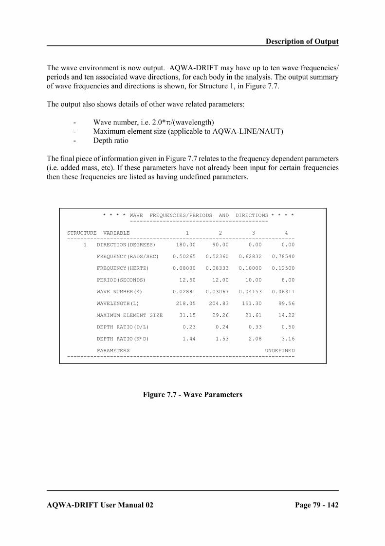
Description of Output
AQWA-DRIFT User Manual 02 Page 79 - 142
* * * * WAVE FREQUENCIES/PERIODS AND DIRECTIONS * * * * ------------------------------------------
STRUCTURE VARIABLE 1 2 3 4 --------------------------------------------------------------------- 1 DIRECTION(DEGREES) 180.00 90.00 0.00 0.00
FREQUENCY(RADS/SEC) 0.50265 0.52360 0.62832 0.78540
FREQUENCY(HERTZ) 0.08000 0.08333 0.10000 0.12500
PERIOD(SECONDS) 12.50 12.00 10.00 8.00
WAVE NUMBER(K) 0.02881 0.03067 0.04153 0.06311 WAVELENGTH(L) 218.05 204.83 151.30 99.56
MAXIMUM ELEMENT SIZE 31.15 29.26 21.61 14.22
DEPTH RATIO(D/L) 0.23 0.24 0.33 0.50
DEPTH RATIO(K*D) 1.44 1.53 2.08 3.16
PARAMETERS UNDEFINED ---------------------------------------------------------------------
The wave environment is now output. AQWA-DRIFT may have up to ten wave frequencies/periods and ten associated wave directions, for each body in the analysis. The output summaryof wave frequencies and directions is shown, for Structure 1, in Figure 7.7.
The output also shows details of other wave related parameters:
- Wave number, i.e. 2.0*B/(wavelength) - Maximum element size (applicable to AQWA-LINE/NAUT) - Depth ratio
The final piece of information given in Figure 7.7 relates to the frequency dependent parameters(i.e. added mass, etc). If these parameters have not already been input for certain frequenciesthen these frequencies are listed as having undefined parameters.
Figure 7.7 - Wave Parameters

Description of Output
AQWA-DRIFT User Manual 02 Page 80 - 142
HYDRODYNAMIC PARAMETERS FOR STRUCTURE 1 - - - - - - - - - - - - - - - - - - - -
AT THE FREE-FLOATING EQUILIBRIUM POSITION ----------------------------------------
BUOYANCY FORCE . . . . . . . . . . . . = 3.2566E+09
Z POSITION OF THE CENTRE OF GRAVITY . = -1.0620E+01
STIFFNESS MATRIX ----------------
X Y Z RX RY RZ --------------------------------------------------------------------------
X 0.0000E+00 0.0000E+00 0.0000E+00 0.0000E+00 0.0000E+00 0.0000E+00
Y 0.0000E+00 0.0000E+00 0.0000E+00 0.0000E+00 0.0000E+00 0.0000E+00
Z 0.0000E+00 0.0000E+00 8.1414E+07 -7.8525E+01 -7.8525E+01 0.0000E+00
RX 0.0000E+00 0.0000E+00 -7.8525E+01 2.4408E+10 0.0000E+00 9.4230E+02
RY 0.0000E+00 0.0000E+00 -7.8525E+01 0.0000E+00 2.4408E+10 2.6698E+03
RZ 0.0000E+00 0.0000E+00 0.0000E+00 0.0000E+00 0.0000E+00 0.0000E+00
7.3 DESCRIPTION OF FLUID LOADING
This information is only output when starting at Stage 1 or 2, or when the PRDL option is usedto echo the information from backing file from AQWA-LINE.
The output detailing the various types of fluid loadings will now be described and this is doneby way of the different categories of loading.
7.3.1 Hydrostatic Stiffness
The hydrostatic stiffness matrix output by AQWA-DRIFT, when printing from backing file, isin the analysis position used in AQWA-LINE for the diffraction/radiation analysis. An exampleoutput is shown in Figure 7.8.
Figure 7.8 - Hydrostatic Stiffness Matrix Output
If used independently, the stiffness matrix output is the sum of the (hydrostatic) stiffness and theadditional stiffness input by the user.

Description of Output
AQWA-DRIFT User Manual 02 Page 81 - 142
* * * * HYDRODYNAMIC PARAMETERS FOR STRUCTURE 1 * * * * -------------------------------------------
WAVE PERIOD = 12.500 WAVE FREQUENCY = 0.5027
ADDED MASS -----------
X Y Z RX RY RZ ------------------------------------------------------------------------
X 9.5594E+06 0.0000E+00 0.0000E+00 0.0000E+00 5.1529E+08 0.0000E+00
Y 0.0000E+00 4.6946E+07 0.0000E+00 -1.0001E+08 0.0000E+00 0.0000E+00
Z 0.0000E+00 0.0000E+00 1.3339E+08 0.0000E+00 0.0000E+00 0.0000E+00
RX 0.0000E+00 -1.0001E+08 0.0000E+00 1.4296E+10 0.0000E+00 0.0000E+00
RY 5.1529E+08 0.0000E+00 0.0000E+00 0.0000E+00 2.3278E+11 0.0000E+00
RZ 0.0000E+00 0.0000E+00 0.0000E+00 0.0000E+00 0.0000E+00 8.0089E+10
7.3.2 Added Mass and Wave Damping
The added mass and wave damping are functions of wave frequency and are therefore output forall specified values of frequency or period. The added mass and wave damping are expressed inmatrix form and Figure 7.9 shows a typical added mass matrix, for Structure 1, at a singlefrequency (wave damping being output in a similar fashion). Summary tables of variation ofadded mass and wave damping with wave frequency/period are also output.
Figure 7.9 - Added Mass Matrix Output

Description of Output
AQWA-DRIFT User Manual 02 Page 82 - 142
7.3.3 Oscillatory Wave Excitation Forces
The wave loading output from AQWA-LINE is presented in tabular form for all the directionsand frequencies specified by the user. The output gives the variation of wave force/moment withfrequency, for each direction (see Figure 7.10). Output is also given with the wave force/momentvarying with direction, for each frequency.
The wave forces/moments are output in terms of amplitude and phase. The phase is related tothe incident wave form (see Appendix C of the AQWA Reference Manual). The waveforces/moments are divided into their various components, and output in terms of the following:
- Froude-Krylov forces/moments - Diffraction forces/moments - Total wave forces/moments
Figure 7.10 shows only the Froude-Krylov component, but the other forces are output in asimilar format.

Description of Output
AQWA-DRIFT User Manual 02 Page 83 - 142
* * * * HYDRODYNAMIC PARAMETERS FOR STRUCTURE 1 * * * * -------------------------------------------
FROUDE KRYLOV FORCES-VARIATION WITH WAVE PERIOD/FREQUENCY ---------------------------------------------------------
PERIOD FREQ DIRECTION X Y Z ------ ----- --------- ----------------------------------------------------- (SECS)(RAD/S)(DEGREES) AMP PHASE AMP PHASE AMP PHASE ----------------------------------------------------------------------------
12.50 0.503 180.00 7.54E+06 90.00 1.21E+00 -79.95 2.26E+07 0.00 12.00 0.524 6.75E+06 90.00 2.36E+00 -90.60 1.85E+07 0.00 10.00 0.628 6.08E+05 90.00 6.77E-01 -107.19 1.04E+05 0.00 8.00 0.785 7.41E+06 -90.00 1.27E+00 112.93 8.64E+06 -180.00 7.00 0.898 1.36E+06 -90.00 1.28E+00 94.29 1.90E+05 -180.00
12.50 0.503 90.00 1.41E+00 -92.53 1.73E+07 -90.00 5.43E+07 0.00 12.00 0.524 1.37E+00 -90.00 1.80E+07 -90.00 5.25E+07 0.00 10.00 0.628 1.58E+00 -101.42 2.10E+07 -90.00 4.26E+07 0.00 8.00 0.785 1.67E+00 -92.15 2.18E+07 -90.00 2.61E+07 0.00 7.00 0.898 1.45E+00 -89.38 1.75E+07 -90.00 1.48E+07 0.00
..........(output line continued below)...........
RX RY RZ ----------------------------------------------------- AMP PHASE AMP PHASE AMP PHASE -----------------------------------------------------
1.81E+01 120.91 1.90E+09 90.00 7.29E+01 171.28 2.14E+01 95.88 1.84E+09 90.00 1.54E+02 -119.43 1.50E+00 -2.98 1.24E+09 90.00 9.61E+01 171.70 7.11E+00 61.58 1.45E+08 -90.00 3.76E+01 -159.58 7.45E+00 -89.28 4.17E+08 -90.00 6.30E+01 19.81 ..... 2.44E+08 90.00 2.57E+02 -111.28 7.57E+01 15.25 2.52E+08 90.00 2.32E+02 -58.88 7.61E+01 9.06 2.85E+08 90.00 4.18E+02 -147.76 1.29E+02 30.27 3.02E+08 90.00 2.87E+02 -93.70 1.65E+02 6.63 2.81E+08 90.00 1.73E+02 -96.82 1.82E+02 14.20
Figure 7.10 - Froude Krylov Forces/Moments

Description of Output
AQWA-DRIFT User Manual 02 Page 84 - 142
* * * * WAVE-DRIFT LOADS FOR UNIT AMPLITUDE/VELOCITY * * * * ------------------------------------------------
* * * * FOR STRUCTURE 1 * * * * -----------------
FORCES FREQUENCY DIRECTION(DEGREES) ------ --------- ------------------ DUE TO (RADIANS/SEC) 90.0 180.0 ------ ------------- ---------------- DRIFT ----- SURGE(X) 0.503 2.92E-02 -1.27E+03 0.524 6.97E-02 -4.25E+03 0.628 5.20E-02 -9.63E+04 0.785 -1.71E-02 -1.81E+05 0.898 -2.34E-02 -2.08E+05 SWAY(Y) 0.503 5.93E+04 -4.63E-04 0.524 1.19E+06 -4.63E-04 0.628 6.74E+05 1.09E-02 0.785 7.77E+05 3.66E-02 0.898 7.14E+05 1.74E-02 YAW(RZ) 0.503 -2.27E+00 -1.02E+00 0.524 -1.09E+01 -2.12E+00 0.628 9.80E+00 -1.08E+00 0.785 -3.58E+00 1.80E-02 0.898 -9.90E+00 -2.04E+00
7.3.4 Mean Wave Drift Forces
The mean wave drift forces and moments as a function of wave period and direction are outputas shown in Figure 7.11. They are given for each body and for the range of user specifiedfrequencies.
Note that the mean wave drift forces are proportional to wave amplitude squared and are givenfor unit wave amplitude.
Figure 7.11 - Mean Wave Drift Forces/Moment

Description of Output
AQWA-DRIFT User Manual 02 Page 85 - 142
* * * * NATURAL FREQUENCIES/PERIODS FOR STRUCTURE 1 * * * * ----------------------------------------------
N.B. THESE NATURAL FREQUENCIES DO *NOT* INCLUDE STIFFNESS DUE TO MOORING LINES.
FREQUENCY UNDAMPED NATURAL FREQUENCIES (RADIANS/SECOND)
NUMBER (RAD/S) SURGE(X) SWAY(Y) HEAVE(Z) ROLL(RX) PITCH(RY) YAW(RZ) ---------------------------------------------------------------------------
1 0.349 0.000 0.000 0.381 0.232 0.238 0.000 2 0.628 0.000 0.000 0.381 0.233 0.238 0.000
PERIOD UNDAMPED NATURAL PERIOD (SECONDS)
NUMBER (SECONDS) SURGE(X) SWAY(Y) HEAVE(Z) ROLL(RX) PITCH(RY) YAW(RZ) ---------------------------------------------------------------------------
1 18.00 0.00 0.00 16.51 27.04 26.42 0.00 2 10.00 0.00 0.00 16.51 27.01 26.39 0.00
FREQUENCY APPROXIMATE PERCENTAGE CRITICAL DAMPING
NUMBER (RAD/S) SURGE(X) SWAY(Y) HEAVE(Z) ROLL(RX) PITCH(RY) YAW(RZ) ---------------------------------------------------------------------------
1 0.349 0.0 0.0 4.5 0.1 0.1 0.0 2 0.628 0.0 0.0 0.7 0.4 0.4 0.0
7.4 FREE FLOATING NATURAL FREQUENCIES AND RESPONSE AMPLITUDE OPERATORS
7.4.1 Natural Frequencies/Periods
AQWA-DRIFT calculates the uncoupled natural frequency/period, for each structure, at eachuser specified wave frequency (added mass being a function of wave frequency).
The damping values of the body motions are compared with, and expressed as a percentage of,critical damping values (see Figure 7.12).
Figure 7.12 - Natural Frequencies/Periods

Description of Output
AQWA-DRIFT User Manual 02 Page 86 - 142
7.4.2 Response Amplitude Operators
The Response Amplitude Operators (which are not required to calculate the wave/drift frequencymotion) will be output as zero if the user has not specified them in Deck 7, unless the user hasused the CRNM option (Calculate RAOs with No Moorings). If they are printed from anAQWA-LINE backing file they will be those calculated by AQWA-LINE.
The output gives the variation of RAOs with frequency, for each direction (see Figure 7.13).Output is also given with the RAOs varying with direction, for each frequency.
The RAOs are output in terms of amplitude and phase, the phase being related to the incidentwave form (see Appendix C of the AQWA Reference Manual).
N.B. These RAOs, which do not include the effect of mooring lines specified in Deck 14, arelabelled as 'R.A.O.S - VARIATION WITH WAVE PERIOD/FREQUENCY' (seeFigure 7.13). If the user has used the CRAO option (Calculate RAOs) then the RAOsare appropriate to each structure in turn with other structures held stationary and arelabelled as 'RECALCULATED R.A.O.S - VARIATION WITH WAVE PERIOD/FREQUENCY'. This is because, in general, the frequencies and directions for eachstructure are not the same, and are therefore incompatible with output in this format.RAOs for the fully coupled system are output, for one direction associated with aparticular spectrum, and are described in Section 7.6.

Description of Output
AQWA-DRIFT User Manual 02 Page 87 - 142
* * * * HYDRODYNAMIC PARAMETERS FOR STRUCTURE 1 * * * * -------------------------------------------
R.A.O.S-VARIATION WITH WAVE PERIOD/FREQUENCY --------------------------------------------
PERIOD FREQ DIRECTION X Y Z ------ ----- --------- ----------------------------------------------------- (SECS)(RAD/S)(DEGREES) AMP PHASE AMP PHASE AMP PHASE ----------------------------------------------------------------------------
18.00 0.349 0.00 0.7050 90.30 0.0054 9.06 2.0916 12.50 10.00 0.628 0.1969 53.44 0.0000 -155.94 0.0299 105.64
18.00 0.349 45.00 0.5089 89.82 0.5107 88.57 2.0932 11.52 10.00 0.628 0.1849 73.61 0.1850 73.64 0.0328 103.52
18.00 0.349 90.00 0.0059 -170.15 0.7066 87.96 2.0942 10.56 10.00 0.628 0.0001 -69.17 0.1969 48.85 0.0299 100.99
..........(output line continued below)...........
RX RY RZ ----------------------------------------------------- AMP PHASE AMP PHASE AMP PHASE -----------------------------------------------------
0.1602 -166.46 0.2060 145.33 0.0276 89.86 0.0016 -79.15 0.0082 155.97 0.0072 52.69
0.2010 -141.76 0.1814 158.61 0.0398 89.19 0.0161 87.23 0.0203 -90.09 0.0136 72.88
0.2350 -133.21 0.1734 -170.51 0.0276 88.43 0.0099 -41.82 0.0014 -73.62 0.0072 48.07
Figure 7.13 - Response Amplitude Operators

Description of Output
AQWA-DRIFT User Manual 02 Page 88 - 142
4 TIMES SQUARE ROOT OF RASTER AREA (S.W.H.) = 3.902
NUMBER WAVE NUMBER FREQUENCY PHASE ORDINATES
1 9.8792E-03 0.3090 0.0028 1.1475
2 1.0706E-02 0.3225 47.3536 1.6838
3 1.1357E-02 0.3326 272.0179 2.0824
4 1.1924E-02 0.3411 165.1140 2.3971
5 1.2442E-02 0.3486 191.7962 2.6514
6 1.2928E-02 0.3555 78.8253 2.8589
7 1.3394E-02 0.3620 16.9361 3.0284
8 1.3845E-02 0.3681 244.3913 3.1661
9 1.4287E-02 0.3740 244.5467 3.2766
10 1.4724E-02 0.3797 336.4894 3.3637
45 4.8742E-02 0.6914 234.5467 0.7391
46 5.2786E-02 0.7195 26.1669 0.6187
47 5.7912E-02 0.7536 227.3885 0.5011
48 6.4732E-02 0.7967 318.4946 0.3870
49 7.4474E-02 0.8546 98.1756 0.2777
50 9.0196E-02 0.9405 157.1081 0.1746
7.5 SPECTRAL LINE PRINTOUT
The program outputs the frequency and the spectral density of each of the discrete spectral linesthat form the wave spectrum, in the form shown in Figure 7.14. The printout shows the wavenumber, frequency, random phase number and spectral density, for each spectral line. By takingfour times the square root of the sum of the contributions from each of the raster lines, theprogram provides an exact indication of the significant wave height (S.W.H.) of the definedspectrum.
Figure 7.14 - Wave Spectral Lines

Description of Output
AQWA-DRIFT User Manual 02 Page 89 - 142
7.6 TIME HISTORY AND FORCE PRINTOUT
At each requested timestep, the full description of the position of the structure and the magnitudeof all relevant forces is printed on the output listing. Figure 7.15 shows a typical example.
The example printout is record number 21 of a simulation, i.e. it is a description of the state ofaffairs at the twenty first timestep of the run and occurs at a time of 100 seconds.
The printout refers to Structure 1, which has three degrees of freedom active, i.e. surge, heaveand pitch. When degrees of freedom are deactivated, there is no printout for that freedom unlessthere are user requested nodes or tensions being printed in which case the X,Y,Z and any otheractive freedoms are printed.
The value of each variable is stated in the chosen set of consistent units and are with respect tothe Fixed Reference Axis System.

Description of Output
AQWA-DRIFT User Manual 01/11/95 Page 90 - 142
JOB TITLE-MODIFIED TEST 20 (FLOATING BOX, 40M DRAUGHT) ------------------------------------------------------------------------------------------------------------------------------- D E G R E E O F F R E E D O M RECORD NO. STRUCTURE POSITION, FORCES NUMBER AND MOMENTS AT X Y Z RX RY RZ
TIME (SECS) CENTRE OF GRAVITY SURGE SWAY HEAVE ROLL PITCH YAW ------------------------------------------------------------------------------------------------------------------------------- RECORD NO. 21 100.00 1 POSITION 0.3857 0.0000 -16.9777 0.0000 -0.3786 0.0000 VELOCITY 0.8794 0.0000 2.3170 0.0000 0.1104 0.0000 ACCELERATION 0.0000 0.0000 0.0000 0.0000 0.0000 0.0000 RAO BASED POSITION -1.5131 0.0000 -6.3577 0.0000 -0.3786 0.0000 RAO BASED VELOCITY 0.7749 0.0000 2.3170 0.0000 0.1104 0.0000 WAVE FREQ POSITION 1.5131 0.0000 6.3577 0.0000 0.3786 0.0000 WAVE FREQ VELOCITY -0.7749 0.0000 -2.3170 0.0000 -0.1104 0.0000 WAVE FREQ ACCEL 0.0000 0.0000 0.0000 0.0000 0.0000 0.0000 SLOW POSITION 1.8988 0.0000 -10.6200 0.0000 0.0000 0.0000 SLOW VELOCITY 0.1045 0.0000 0.0000 0.0000 0.0000 0.0000 SLOW ACCEL 0.0000 0.0000 0.0000 0.0000 0.0000 0.0000 MOORING -9.9028E+05 0.0000E+00 4.4670E+05 -4.0000E+00 -6.2262E+06 -8.5938E-02 LINEAR DAMPING -3.0504E+07 2.3105E-01 -4.4610E+07 1.6727E-01 2.7668E+07 -6.0535E-05 DRIFT 3.6214E+06 5.2877E-02 0.0000E+00 0.0000E+00 0.0000E+00 -1.2570E+01 GRAVITY 0.0000E+00 0.0000E+00 -3.2566E+09 0.0000E+00 0.0000E+00 0.0000E+00 CURRENT DRAG -3.2215E+04 -2.7797E-09 0.0000E+00 0.0000E+00 0.0000E+00 0.0000E+00 HYDROSTATIC 0.0000E+00 0.0000E+00 3.7742E+09 -8.2009E+02 1.6130E+08 0.0000E+00 WIND -1.4415E+01 -1.2438E-12 0.0000E+00 0.0000E+00 0.0000E+00 0.0000E+00 THRUSTER 0.0000E+00 0.0000E+00 0.0000E+00 0.0000E+00 0.0000E+00 0.0000E+00 YAW DRAG 0.0000E+00 0.0000E+00 0.0000E+00 0.0000E+00 0.0000E+00 0.0000E+00 WAVE FREQ FORCE 1.2676E+08 1.3466E+01 1.0230E+08 -1.1802E+02 4.1145E+07 1.3792E+00 ERROR PER TIMESTEP 0.0000E+00 0.0000E+00 0.0000E+00 0.0000E+00 0.0000E+00 0.0000E+00 TOTAL REACTION FORCE 0.0000E+00 0.0000E+00 0.0000E+00 0.0000E+00 0.0000E+00 0.0000E+00 TOTAL FORCE 9.8852E+07 1.3750E+01 5.7575E+08 -9.4194E+02 2.2389E+08 -1.1277E+01
TENSION LINE 1 1.2745E+06 3.9454E-03 7.6713E+04 TOTAL TENSION 1.2768E+06 TENSION LINE 2 -5.5078E+03 1.7629E+06 1.1097E+05 TOTAL TENSION 1.7664E+06 TENSION LINE 3 -2.2537E+06 6.1715E-03 1.4804E+05 TOTAL TENSION 2.2586E+06 TENSION LINE 4 -5.5078E+03 -1.7629E+06 1.1097E+05 TOTAL TENSION 1.7664E+06
Figure 7.15 - Timestep Printout

Description of Output
AQWA-DRIFT User Manual 02 Page 91 - 142
The following describes each of the variables:
1. POSITION
Total position of structure centre of gravity in the Fixed Reference Axis
2. VELOCITY
Total velocity of structure centre of gravity in the Fixed Reference Axis
3. ACCELERATION
Total acceleration of structure centre of gravity in the Fixed Reference Axis
4. RAO BASED POSITION
FAST position of structure centre of gravity calculated by summing the real partof the product of complex response amplitude operator and the wave spectrumfor each frequency forming the wave spectrum.
5. RAO BASED VELOCITY
FAST velocity of structure centre of gravity calculated by summing the real partof the product of complex response amplitude operator of velocity and the wavespectrum for each frequency which forms the wave spectrum.
7. WAVE FREQ POSITION
Rapidly varying part of total position filtered from POSITION
8. WAVE FREQ VELOCITY
Rapidly varying part of total velocity filtered from VELOCITY
9. WAVE FREQ ACCEL
Rapidly varying part of total acceleration filtered from ACCELERATION
10. SLOW POSITION
Slowly varying part of total position filtered from POSITION
11. SLOW VELOCITY
Slowly varying part of total velocity filtered from VELOCITY

Description of Output
AQWA-DRIFT User Manual 02 Page 92 - 142
12. SLOW ACCEL
Slowly varying part of total acceleration filtered from ACCELERATION
14. MOORING
The total force and moments on the structure due to all the mooring lines,catenaries and hawsers
17. LINEAR DAMPING
The total linear damping force
19. DRIFT
The total second order drift force on structure
21. GRAVITY
The total gravity force on structure
22. CURRENT DRAG
The total drag force on structure due to relative current
24. HYDROSTATIC
The total hydrostatic force on structure
25. WIND
The total drag force on structure due to relative wind
27. THRUSTER
The total force on structure due to all applied thruster forces
28. YAW DRAG
The drag on the structure due to its yaw velocity
29. WAVE FREQ FORCE
The total diffraction and Froude Krylov force on the structure
30. ERROR PER TIMESTEP

Description of Output
AQWA-DRIFT User Manual 02 Page 93 - 142
The maximum error in the position for the present timestep
31. TOTAL REACTION FORCE
The total reaction force due to articulations on each structure
50. TOTAL FORCE
The sum total of all forces applied to the structure

Description of Output
AQWA-DRIFT User Manual 02 Page 94 - 142
7.7 STATISTICS PRINTOUT
At the end of the simulation timestep printout, those parameters which have been printed at eachtimestep are then analysed statistically over the whole length of the simulation. The results aretabulated in the form shown in Figure 7.16.
This example shows the statistics for the position of Structure 1. For each of the active degreesof freedom, the following are calculated.
MEAN VALUE the sum of all the values divided by the number of timesteps
2 x R.M.S two times the root mean squared value. This is often termed thesignificant value
MEAN HIGHEST + the mean value of the highest third positive and1/3 PEAKS - negative peaks. For simulation of a linear system this should be
equal to twice the root mean square. A large difference betweenthis value and the significant value is an indication that thevariation of the parameter is not following a normal distribution.A large difference between the values for positive and negativepeaks is an indication of skewness or asymmetry of variation.
MAXIMUM PEAKS + the three maximum peak values
MINIMUM PEAKS - the three minimum peak values
The values of each parameter are sorted into small ranges (or bins) covering the total range ofvariation. For example, in Figure 7.16, the X or surge position is greater than 3.2 and less orequal to 3.8 for 4 percent of the time.

Description of Output
AQWA-DRIFT User Manual 02 Page 95 - 142
STRUCTURE 1 POSITION OF COG -------------------------------
---------------------------------------------------------------------- SURGE(X) SWAY(Y) HEAVE(Z)----------------------------------------------------------------------
MEAN VALUE 1.5484 0.0000 -10.5363
2 x R.M.S 2.7670 0.0000 9.2783
MEAN HIGHEST + 2.9586 0.0000 9.2706 1/3 PEAKS - -2.2109 0.0000 -9.1744
MAXIMUM PEAKS + 4.9162 0.0000 -1.1053 4.0976 0.0000 -1.4260 2.9995 0.0000 -3.4676
MINIMUM PEAKS - -0.9920 0.0000 -20.3015 -0.5930 0.0000 -19.1198 -0.5785 0.0000 -16.9777
----------- ---------------------------------------------------- PROBABILITY RANGE PER CENT RANGE PER CENT RANGE PER CENT DISTRIBUTION LIMITS OCCUR LIMITS OCCUR LIMITS OCCUR ----------- ---------------------------------------------------- -1.000 0.000 -24.000 10.0 0.0 0.0 -0.400 0.000 -21.600 11.0 3.0 2.0 0.200 0.000 -19.200 11.0 1.0 7.0 0.800 0.000 -16.800 14.0 3.0 11.0 1.400 0.000 -14.400 14.0 2.0 20.0 2.000 0.000 -12.000 23.0 14.0 16.0 2.600 0.000 -9.600 5.0 22.0 20.0 3.200 0.000 -7.200 4.0 33.0 11.0 3.800 0.000 -4.800 4.0 22.0 7.0 4.400 0.000 -2.400 4.0 0.0 6.0 5.000 0.000 0.000
Figure 7.19 - Statistics Summary

Example of Program Use
AQWA-DRIFT User Manual 02 Page 96 - 142
CHAPTER 8 - EXAMPLE OF PROGRAM USE
In this chapter, an example problem using AQWA-DRIFT is illustrated. The problem is one inwhich AQWA-LINE has been used to perform the analysis Stages 1 to 3. All steps in thesubsequent analysis procedure are clearly shown, from the problem definition, through the datapreparation, to the final analysis run itself. The method used in this chapter can be easilyfollowed by the user, and if so desired, the user can repeat the whole procedure, using the samedata as used here, to obtain the same results. In this manner, the new user can quickly gainconfidence in using the program.
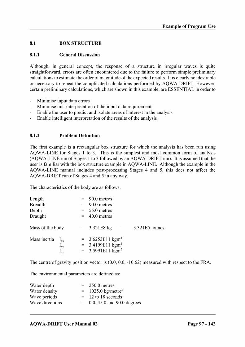
Example of Program Use
AQWA-DRIFT User Manual 02 Page 97 - 142
8.1 BOX STRUCTURE
8.1.1 General Discussion
Although, in general concept, the response of a structure in irregular waves is quitestraightforward, errors are often encountered due to the failure to perform simple preliminarycalculations to estimate the order of magnitude of the expected results. It is clearly not desirableor necessary to repeat the complicated calculations performed by AQWA-DRIFT. However,certain preliminary calculations, which are shown in this example, are ESSENTIAL in order to
- Minimise input data errors- Minimise mis-interpretation of the input data requirements - Enable the user to predict and isolate areas of interest in the analysis - Enable intelligent interpretation of the results of the analysis
8.1.2 Problem Definition
The first example is a rectangular box structure for which the analysis has been run usingAQWA-LINE for Stages 1 to 3. This is the simplest and most common form of analysis(AQWA-LINE run of Stages 1 to 3 followed by an AQWA-DRIFT run). It is assumed that theuser is familiar with the box structure example in AQWA-LINE. Although the example in theAQWA-LINE manual includes post-processing Stages 4 and 5, this does not affect theAQWA-DRIFT run of Stages 4 and 5 in any way.
The characteristics of the body are as follows:
Length = 90.0 metresBreadth = 90.0 metresDepth = 55.0 metresDraught = 40.0 metres
Mass of the body = 3.321E8 kg = 3.321E5 tonnes
Mass inertia Ixx = 3.6253E11 kgm2
Iyy = 3.4199E11 kgm2
Izz = 3.5991E11 kgm2
The centre of gravity position vector is (0.0, 0.0, -10.62) measured with respect to the FRA.
The environmental parameters are defined as:
Water depth = 250.0 metresWater density = 1025.0 kg/metre3
Wave periods = 12 to 18 secondsWave directions = 0.0, 45.0 and 90.0 degrees

Example of Program Use
AQWA-DRIFT User Manual 02 Page 98 - 142
The box structure is moored by horizontal soft moorings attached to the mid-sides of the box atthe water line, as shown in Figure 8.1
Unstretched length of each mooring line = 100.0 metres Stretched length of each mooring line = 101.0 metres Extension of each mooring line = 1.0 metres Stiffness of each mooring line = 1.4715E6 N/m Pre-tension in each mooring line = 1.4715E6 newtons
It is required to obtain the response of the box in irregular waves for a given sea-state, withparticular attention being paid to the hawser tensions. In the first instance, only the driftoscillations of the structure will be investigated. After this has been completed, the effect of thewave frequency forces will be investigated. Note that the analysis is performed using SI units.

Example of Program Use
AQWA-DRIFT User Manual 02 Page 99 - 142
Figure 8.1 - Mooring Lines

Example of Program Use
AQWA-DRIFT User Manual 02 Page 100 - 142
8.1.3 Natural Frequencies
It is good practice when using AQWA-DRIFT to perform some short and simple preliminaryruns to ensure that the model has been formed correctly before embarking on long simulationruns, where errors in modelling may be more difficult to identify.
The first check is to ensure that the model has the correct natural periods. This is achieved byperforming a short run with the structure initially displaced from its still water equilibriumposition and allowing it to oscillate at its natural frequency about the equilibrium position. Theobserved natural periods of the motion can be checked against simple calculations. Since we arerestricting the investigation to the structure's drift motion response, only the natural frequenciesin the horizontal degrees of freedom (surge, pitch, yaw) need be investigated.
In the horizontal freedoms, AQWA-LINE gives no natural frequencies as the hydrostaticstiffness in these freedoms is zero. With the addition of the four mooring lines in thisAQWA-DRIFT analysis, all these freedoms will have stiffness and corresponding naturalfrequencies.
At a frequency of 0.349 rad/sec (period 18 secs) the surge terms on the leading diagonal of theadded mass and stiffness matrices are
Surge added mass inertia = 3.02(108 kg
Surge stiffness = 2.94(106 N/m (2 lines each of 1.47(106 )
The natural frequency squared is therefore 2.94(108 /(3.32(108 + 3.02(108 ) giving a freedomuncoupled natural frequency of 0.0681 rad/sec (natural period 92.2 secs).
At a frequency of 0.349 rad/sec (period 18 secs) the yaw terms on the leading diagonal of theadded mass and stiffness matrices are
Yaw added mass inertia = 1.27(1011 kgm2
Yaw stiffness = 3.84(108 Nm/rad
The yaw stiffness due to each line is given by
K = Td(1+d/L)
whereT = tension
d = distance between CG and attachment point L = line length
Total yaw stiffness = 4 ( 1.47(106 ( 45(1+45/100) = 3.84(108 Nm/rad

Example of Program Use
AQWA-DRIFT User Manual 02 Page 101 - 142
The natural frequency squared is therefore 3.84(108 /( 3.60(10 11 + 1.27(10 11) giving anuncoupled natural frequency of 0.0281 rad/sec (natural period 223.7 secs).
We will see that it is the motions of the structure at these frequencies that will dominate the driftresponse of the structure.
The added mass at low or drift frequency will not generally be the same as that at the lowestwave frequency, but is sufficiently close for the purpose of the calculations above.
8.1.4 Low Frequency Added Mass and Damping
It may be assumed that, at low frequency, the added mass and damping remain constant, asvalues of drift added mass for the horizontal freedoms tend towards finite values at lowfrequency. The values often used are those of the lowest wave frequency input in AQWA-LINE.This is normally a good approximation. The values for the vertical freedoms are also usedbecause no motion at low frequency is expected. However, for damping, empirical values maybe input based on either the experience of the user or experimental results. For this example,values of added mass and damping at a frequency of 0.349 rad/sec (period 18 secs) will be used.Note that for the evaluation of undamped natural periods, no drift damping is used. This appliesto the initial AQWA-DRIFT run.
8.1.5 Hull and Superstructure Loading Coefficients
Data for the hull and superstructure loading coefficients for wind and current in this example arebased on the projected area through the centroid in the three directions specified in Deck 6.
Forces due to the current at 0, 90 degree headings in the X and Y directions respectively (for unitvelocity) are
Force = 0.5 ( Density ( Area ( Drag coefficient ( cos (heading)
= 0.5 ( 1025.0 ( 40.0 ( 90.0 ( 1.6 ( cos (0 ) = 2.95E6 Ns2 /m2
At 45 degrees, in both the X and Y directions, the forces are
= 0.5 ( 1025.0 ( 40.0 ( 127.0 ( 1.3 ( cos (45) = 2.40E6 Ns2 /m2

Example of Program Use
AQWA-DRIFT User Manual 02 Page 102 - 142
The corresponding moments at the centre of gravity (10.62 metres below the waterline, centreof area at Z = -20.0) are 2.95E6 ( 9.38 and 2.40E6 ( 9.38
i.e.
At a heading of 0, Moment = 2.77E7 (-ve in Y, zero in the X direction) At a heading of 45, Moment = 2.25E7 (-ve in Y, +ve in the X direction) At a heading of 90, Moment = 2.77E7 (zero in Y, +ve in the X direction)
The units for the moment coefficients are Ns2 /m.
Similarly, the forces on the superstructure due to the wind at 0, 90 degree headings in the X andY directions respectively (for unit velocity) are:
Force = 0.5 ( 1.22 ( 15.0 ( 90.0 ( 1.6 ( cos (0 ) = 1.32E3 Ns2 /m2
At 45 degrees, in both the X and Y directions, the forces are:
= 0.5 ( 1.22 ( 15.0 ( 127.0 ( 1.3 ( cos (45) = 1.07E3 Ns2 /m2
The corresponding moments at the centre of gravity (10.62 metres below the waterline, centreof area at Z = +7.5) are 1.32E3 ( 18.12 and 1.07E3 ( 18.12
i.e.
At a heading of 0, Moment = 2.39E4 (+ve in Y, zero in the X direction) At a heading of 45, Moment = 1.94E4 (+ve in Y, -ve in the X direction) At a heading of 90, Moment = 2.39E4 (zero in Y, -ve in the X direction)
8.1.6 Sea Spectra, Current and Wind
The following spectrum and its associated directions will be used in the drift and wave frequencyanalyses:
Spectrum Type Frequency Range(radians/sec)
SignificantWave Height
Zero CrossingPeriod
Pierson-Moskowitz 0.3 - 1.0 8.0 11.0
Current and wind will not be applied.

Example of Program Use
AQWA-DRIFT User Manual 02 Page 103 - 142
8.1.7 Specification of the Mooring Lines
The mooring lines are simple linear elastic hawsers and therefore require one line of input datafor each mooring line. Each line contains stiffness, unstretched length, and the structure numbersand node numbers of the two attachments points. For a line joining a structure to a fixed point,the structure number corresponding to the fixed point should be set to zero. The node numbersand their positions, to which the mooring lines are attached, must be input in the coordinate Deck1. Each mooring line of unstretched length 100 metres has a stiffness of 1.47E6 newtons permetre. Each mooring line is pre-tensioned to 1.47E6 newtons (i.e. extended by 1 metre) to givethe structure a significant yaw stiffness.
8.1.8 Start Position for Analysis
If the starting position is offset from the equilibrium position of the structure, there will be atransient response, which will decay to the steady state under the action of the specifieddamping. Such an offset is necessary to investigate the natural period of the structure. However,it is best to keep this offset small, in order to minimise the influence of the initial transient on thestatistics of the complete run.
The equilibrium position given by AQWA-LIBRIUM for the specified spectrum (NB withoutcurrent, wind and thruster forces) is:
Surge (X) Sway (Y) Heave (Z) Roll(RX) Pitch (RY) Yaw (RZ)
0.7425 0.0000 -10.6200 0.0000 -0.0523 0.0000
Only the positions in the horizontal degrees of freedom need be considered.
8.1.9 Time Integration Parameters
The structure's natural periods of oscillation in surge and yaw have been calculated to be 92 and224 seconds. A suitable timestep therefore is 5 seconds (minimum period/20). To determine thenatural period of oscillation, a simulation of about 4 cycles is sufficient. So, for surgeoscillations, 80 timesteps are used. For the complete simulation, 800 timesteps are used.

Example of Program Use
AQWA-DRIFT User Manual 02 Page 104 - 142
8.1.10 Input Preparation For Natural Frequency Data Run
The AQWA-LINE run (see AQWA-LINE example), has been performed and the followinginformation is contained on the RESTART backing file produced by AQWA-LINE:
- input of the node coordinate data- input of the model's element topology with associated material and geometry properties- input of the static environment- the detailed properties of elements used in each body - the final mass and inertia properties of each body- the preliminary diffraction modelling checks- the wave periods and directions- the analysis position of each body- the secondary diffraction modelling checks- hydrostatic calculations for each body- diffraction radiation analysis giving wave loading coefficients
The input decks for the AQWA-DRIFT DATA run are shown in Figure 8.2 and are describedbelow.
Note that the DATA option is equivalent to a program RESTART which starts at the beginningof Stage 4 and finishes at the end of Stage 2.
- JOB card provides identifier program, and type of analysis to be used- TITLE card prescribes a title header for the run- OPTIONS card containing the selected options:
REST - indicates that a restart run is required DATA - selects performance of up to Stage 4 only END - indicates the end of the options list- RESTART card specifies start and finish stages
- Deck 9
Low frequency or drift added mass (values input are at the lowest wave frequency) Zero damping (default) is used for natural frequency calculation The value of yaw rate drag is input
- Deck 10
Wind and current loading coefficients
- Deck 11
This deck has no input and so has a NONE deck header

Example of Program Use
AQWA-DRIFT User Manual 02 Page 105 - 142
- Deck 12
Since only the horizontal degrees of freedom are being used, the heave, roll and pitchfreedoms are de-activated
- Deck 13
This deck has no input and so has a NONE deck header
- Deck 14
Description of each mooring line property and combination
- Deck 15
The structure is given a surge displacement of 1 metre from the origin of the FRA (theequilibrium position for this run)
- Deck 16
The time integration parameters
- Deck 17
This deck has no input and so has a NONE deck header
- Deck 18
Additional output requests concerning the hawser attachment points information at everytenth timestep (default) is required
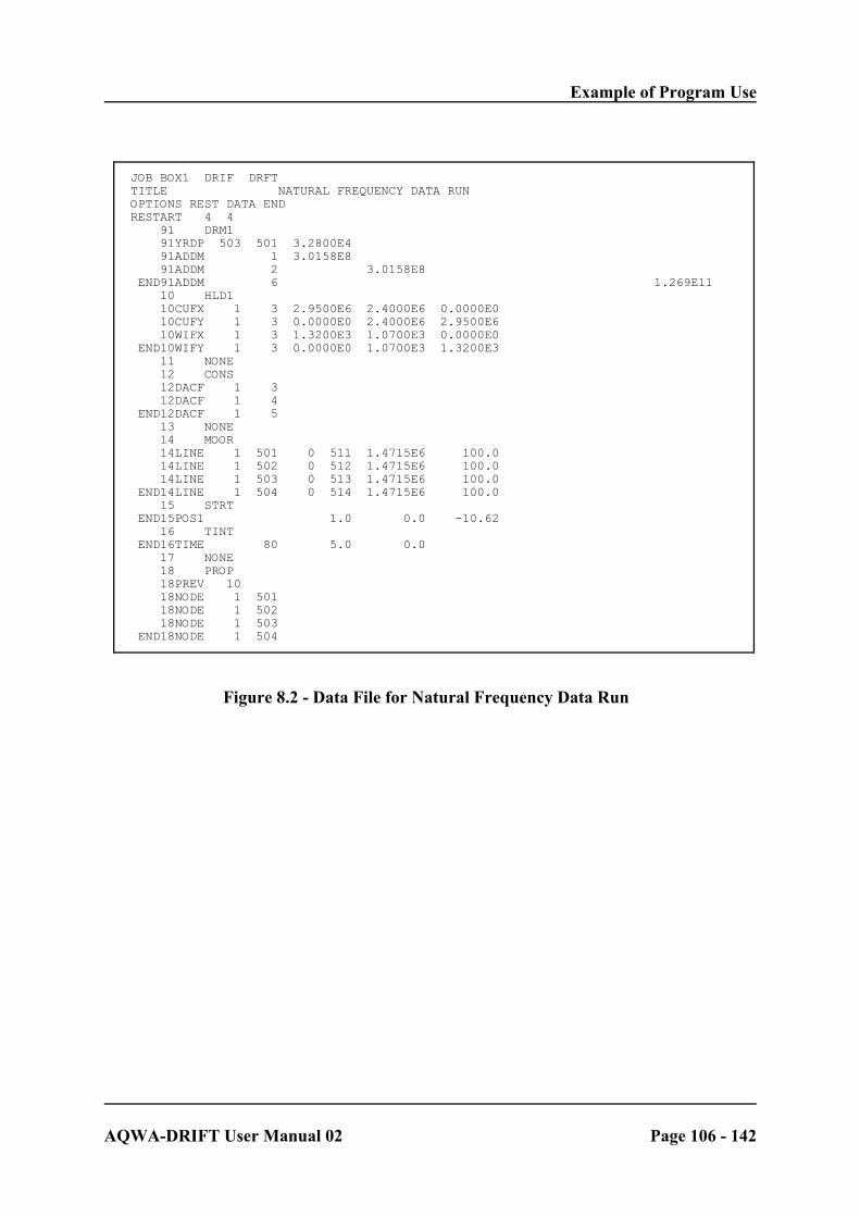
Example of Program Use
AQWA-DRIFT User Manual 02 Page 106 - 142
JOB BOX1 DRIF DRFT TITLE NATURAL FREQUENCY DATA RUN OPTIONS REST DATA END RESTART 4 4 91 DRM1 91YRDP 503 501 3.2800E4 91ADDM 1 3.0158E8 91ADDM 2 3.0158E8 END91ADDM 6 1.269E11 10 HLD1 10CUFX 1 3 2.9500E6 2.4000E6 0.0000E0 10CUFY 1 3 0.0000E0 2.4000E6 2.9500E6 10WIFX 1 3 1.3200E3 1.0700E3 0.0000E0 END10WIFY 1 3 0.0000E0 1.0700E3 1.3200E3 11 NONE 12 CONS 12DACF 1 3 12DACF 1 4 END12DACF 1 5 13 NONE 14 MOOR 14LINE 1 501 0 511 1.4715E6 100.0 14LINE 1 502 0 512 1.4715E6 100.0 14LINE 1 503 0 513 1.4715E6 100.0 END14LINE 1 504 0 514 1.4715E6 100.0 15 STRT END15POS1 1.0 0.0 -10.62 16 TINT END16TIME 80 5.0 0.0 17 NONE 18 PROP 18PREV 10 18NODE 1 501 18NODE 1 502 18NODE 1 503 END18NODE 1 504
Figure 8.2 - Data File for Natural Frequency Data Run

Example of Program Use
AQWA-DRIFT User Manual 02 Page 107 - 142
8.1.11 Output from Natural Frequency Data Run
The DATA run produces the output shown in Figures 8.3 to 8.12, described below.
Figure 8.3 AQWA-DRIFT Header Page used for Identification
Figure 8.4 Card echo (mandatory) for Decks 9 to 18 This is used to check data input
Figure 8.5 Yaw rate drag and Drift Frequency Added mass and Damping An echo of the data input in Deck 9
Figure 8.6 Wind/Current Loads and Thruster ForcesA tabulation of the data input in Deck 10
The omission of thruster forces is also brought to the users attention
Figure 8.7 Constraints
The table shows X, Y, RZ freedoms active Articulations are not yet implemented
Figure 8.8 Cable/Mooring Line Configurations
Tabulation of the mooring lines input in Deck 14 (Note that the cable groupnumber is only applicable to non-linear mooring lines)
Figure 8.9 Initial Conditions of the Centre of Gravity Tabulation of the initial position and velocity input in Deck 15
Figure 8.10 Time Integration Parameters
Details of the simulation length and timestep
The expected errors for the specified timestep are indicated(Note that the errorfor the expected response period of 92 seconds is about 0.3 per cent)
Figure 8.11 Position of User-Requested Nodes
Tabulation of the nodes and their positions input in Deck 18. (Note that thepositions shown are those in the last analysis position input in Deck 15)

Example of Program Use
AQWA-DRIFT User Manual 02 Page 108 - 142
AAAAAA QQQQQQ WW WW AAAAAA DDDDDDD RRRRRR IIII FFFFFFFF TTTTTTTT AAAAAAAA QQQQQQQQ WW WW AAAAAAAA DDDDDDDD RRRRRRRR IIII FFFFFFFF TTTTTTTTTT AA AA QQ QQ WW WW AA AA DD DD RR RR II FF TT AA AA QQ QQ WW WW AA AA DD DD RR RR II FF TT AAAAAAAA QQ QQ WW WW AAAAAAAA IIII DD DD RRRRRRRR II FFFFF TT AAAAAAAA QQ QQ WW WW WW AAAAAAAA IIII DD DD RRRRRRRR II FFFFF TT AA AA QQ QQ WW WW WW AA AA DD DD RRRRR II FF TT AA AA QQ QQ QQ WW WW WW AA AA DD DD RR RRR II FF TT AA AA QQQQQQQQ WWWWWWWWWW AA AA DDDDDDDD RR RRR IIII FF TTTT AA AA QQQQQQ WWWWWWWW AA AA DDDDDDD RR RRR IIII FF TTTT QQ
THE DEVELOPMENT OF THE AQWA SUITE WAS CARRIED OUT BY CENTURY DYNAMICS LIMITED WHO ARE CONTINUALLY IMPROVING THE CAPABILITIES OF THE HYDRODYNAMIC CALCULATIONS AS MORE ADVANCED TECHNIQUES BECOME AVAILABLE. SUGGESTIONS FROM USERS REGARDING DEVELOPMENT WILL BE WELCOMED.
CENTURY DYNAMICS LIMITED DYNAMICS HOUSE 86 HURST ROAD HORSHAM WEST SUSSEX RH12 2DT
JOB TITLE : NATURAL FREQUENCY DATA RUN
Figure 8.3 - AQWA-DRIFT Header Page (used for identification)

Example of Program Use
AQWA-DRIFT User Manual 02 Page 109 - 142
DECK 9 -------
91YRDP 503 501 3.28E+04 0.00E+00 0.00E+00 0.00E+00 0.00E+00 0.00E+00 91ADDM 0 1 3.02E+08 0.00E+00 0.00E+00 0.00E+00 0.00E+00 0.00E+00 91ADDM 0 2 0.00E+00 3.02E+08 0.00E+00 0.00E+00 0.00E+00 0.00E+00 END91ADDM 0 6 0.00E+00 0.00E+00 0.00E+00 0.00E+00 0.00E+00 1.27E+11
DECK 10.1 -------
10CUFX 1 3 2.950E+06 2.400E+06 0.000E+00 0.000E+00 0.000E+00 0.000E+00 10CUFY 1 3 0.000E+00 2.400E+06 2.950E+06 0.000E+00 0.000E+00 0.000E+00 10WIFX 1 3 1.320E+03 1.070E+03 0.000E+00 0.000E+00 0.000E+00 0.000E+00 END10WIFY 1 3 0.000E+00 1.070E+03 1.320E+03 0.000E+00 0.000E+00 0.000E+00
DECK 11 -------
DECK 12 -------
12DACF 1 3 0 0 0 0 0 0 0 12DACF 1 4 0 0 0 0 0 0 0 END12DACF 1 5 0 0 0 0 0 0 0
DECK 13 -------
DECK 14 -------
14LINE 1 501 0 511 1.472E+06 1.000E+02 0.000E+00 0.000E+00 0.000E+00 14LINE 1 502 0 512 1.472E+06 1.000E+02 0.000E+00 0.000E+00 0.000E+00 14LINE 1 503 0 513 1.472E+06 1.000E+02 0.000E+00 0.000E+00 0.000E+00 END14LINE 1 504 0 514 1.472E+06 1.000E+02 0.000E+00 0.000E+00 0.000E+00
DECK 15 -------
END15POS1 1.000 0.000 -10.620 0.000 0.000 0.000
DECK 16 -------
END16TIME 0 80 5.000 0.000 0.000 0.000 0.000 0.000
DECK 17 -------
DECK 18 -------
18PREV 10 0 0 0 18NODE 1 501 0 0 18NODE 1 502 0 0 18NODE 1 503 0 0 END18NODE 1 504 0 0
Figure 8.4 - Card Echo for Decks 9 to 18

Example of Program Use
AQWA-DRIFT User Manual 02 Page 110 - 142
H Y D R O D Y N A M I C P A R A M E T E R S F O R S T R U C T U R E 1 - - - - - - - - - - - - - - - - - - - - - - - - - - - - - - - - - - - - - - -
YAW-RATE DRAG CONSTANT. . . . . . . . . . . . = 32800.000
NEGATIVE X COORDINATE OF VESSEL EXTREMITY . . = -45.000
POSITIVE X COORDINATE OF VESSEL EXTREMITY . . = 45.000
ADDED MASS AT DRIFT FREQUENCY -----------------------------
X Y Z RX RY RZ ---------------------------------------------------------------------------------
X 3.0158E+08 0.0000E+00 0.0000E+00 0.0000E+00 0.0000E+00 0.0000E+00
Y 0.0000E+00 3.0158E+08 0.0000E+00 0.0000E+00 0.0000E+00 0.0000E+00
Z 0.0000E+00 0.0000E+00 0.0000E+00 0.0000E+00 0.0000E+00 0.0000E+00
RX 0.0000E+00 0.0000E+00 0.0000E+00 0.0000E+00 0.0000E+00 0.0000E+00
RY 0.0000E+00 0.0000E+00 0.0000E+00 0.0000E+00 0.0000E+00 0.0000E+00
RZ 0.0000E+00 0.0000E+00 0.0000E+00 0.0000E+00 0.0000E+00 1.2690E+11
DAMPING AT DRIFT FREQUENCY --------------------------
X Y Z RX RY RZ ---------------------------------------------------------------------------------
X 0.0000E+00 0.0000E+00 0.0000E+00 0.0000E+00 0.0000E+00 0.0000E+00
Y 0.0000E+00 0.0000E+00 0.0000E+00 0.0000E+00 0.0000E+00 0.0000E+00
Z 0.0000E+00 0.0000E+00 0.0000E+00 0.0000E+00 0.0000E+00 0.0000E+00
RX 0.0000E+00 0.0000E+00 0.0000E+00 0.0000E+00 0.0000E+00 0.0000E+00
RY 0.0000E+00 0.0000E+00 0.0000E+00 0.0000E+00 0.0000E+00 0.0000E+00
RZ 0.0000E+00 0.0000E+00 0.0000E+00 0.0000E+00 0.0000E+00 0.0000E+00
Figure 8.5 - Drift Frequency Added Mass and Damping

Example of Program Use
AQWA-DRIFT User Manual 02 Page 111 - 142
W I N D / C U R R E N T L O A D S F O R U N I T A M P L I T U D E / V E L O C I T Y - - - - - - - - - - - - - - - - - - - - - - - - - - - - - - - - - - - - - - - - - - - - - - A N D T H R U S T E R F O R C E S F O R S T R U C T U R E 1 - - - - - - - - - - - - - - - - - - - - - - - - - - - - - - - - - - -
NO THRUSTER FORCES --------------------
FORCES FREQUENCY DIRECTION(DEGREES) (SURGE=COS SWAY=SIN HEAVE=COS) (ROLL=SIN PITCH=COS YAW=SIN) ------ --------- ----------------------------------------------- DUE TO (RADIANS/SEC) 0.0 45.0 90.0 ------ ------------- --------------------------
WIND ---- SURGE(X) 1.32E+03 1.07E+03 0.00E+00 SWAY(Y) 0.00E+00 1.07E+03 1.32E+03 HEAVE(Z) 0.00E+00 0.00E+00 0.00E+00 ROLL(RX) 0.00E+00 0.00E+00 0.00E+00 PITCH(RY 0.00E+00 0.00E+00 0.00E+00 YAW(RZ) 0.00E+00 0.00E+00 0.00E+00
CURRENT ------- SURGE(X) 2.95E+06 2.40E+06 0.00E+00 SWAY(Y) 0.00E+00 2.40E+06 2.95E+06 HEAVE(Z) 0.00E+00 0.00E+00 0.00E+00 ROLL(RX) 0.00E+00 0.00E+00 0.00E+00 PITCH(RY 0.00E+00 0.00E+00 0.00E+00 YAW(RZ) 0.00E+00 0.00E+00 0.00E+00
Figure 8.6 - Wind/Current Loads and Thruster Forces
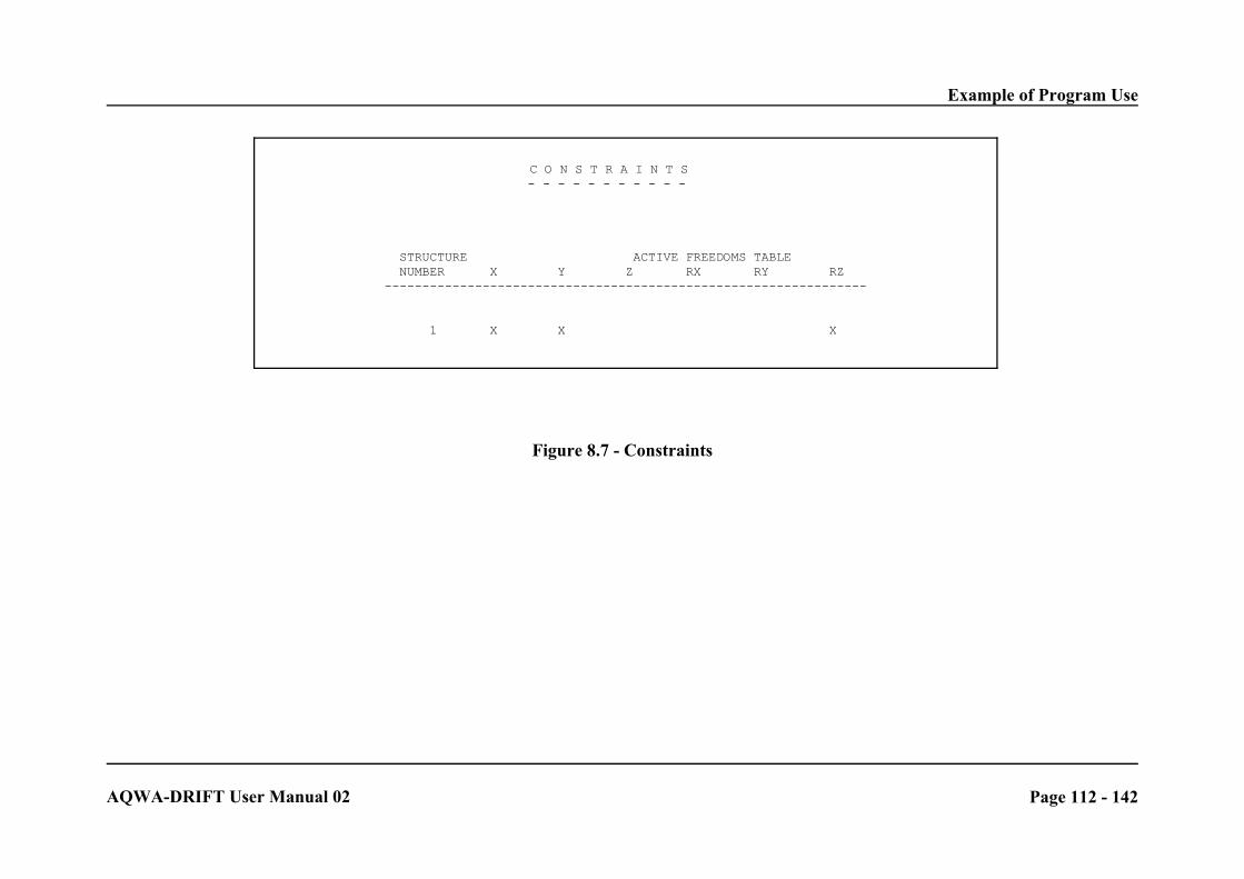
Example of Program Use
AQWA-DRIFT User Manual 02 Page 112 - 142
C O N S T R A I N T S - - - - - - - - - - -
STRUCTURE ACTIVE FREEDOMS TABLE NUMBER X Y Z RX RY RZ ----------------------------------------------------------------
1 X X X
Figure 8.7 - Constraints

Example of Program Use
AQWA-DRIFT User Manual 02 Page 113 - 142
C A B L E / M O O R I N G L I N E C O N F I G U R A T I O N S - - - - - - - - - - - - - - - - - - - - - - - - - - - - - - - - -
+ CABLE ATTACHMENTS( STRUCTURE - 0 - IS GROUND) ---------------------------------------------
COMBINATION CABLE CABLE CABLE ATTACHED TO AT NODE LINKED TO AT NODE UNSTRETCHED FORCE OR + NUMBER NUMBER GROUP TYPE STRUCTURE NUMBER STRUCTURE NUMBER LENGTH STIFFNESS ---------------------------------------------------------------------------------------------------------
1 1 0 LIN ELASTIC 1 501 0 511 100.000 0.147E+07
2 0 LIN ELASTIC 1 502 0 512 100.000 0.147E+07
3 0 LIN ELASTIC 1 503 0 513 100.000 0.147E+07
4 0 LIN ELASTIC 1 504 0 514 100.000 0.147E+07
Figure 8.8 - Cable/Mooring Line Configurations

Example of Program Use
AQWA-DRIFT User Manual 02 Page 114 - 142
I N I T I A L P O S I T I O N A N D V E L O C I T Y O F T H E - - - - - - - - - - - - - - - - - - - - - - - - - - - - - - - - - - - -
C E N T E R O F G R A V I T Y - - - - - - - - - - - - - - - - -
STRUCTURE PARAMETER TRANSLATIONS(FRA) ROTATIONS(FRA) DIRECTION COSINES
NUMBER X Y Z RX RY RZ X Y Z ----------------------------------------------------------------------------------------------------------------------------
1 POSITION 1.000 0.000 -10.620 0.000 0.000 0.000 1.0000 0.0000 0.0000
0.0000 1.0000 0.0000
0.0000 0.0000 1.0000
1 VELOCITY 0.000 0.000 0.000 0.000 0.000 0.000
----------------------------------------------------------------------------------------------------------------------------
Figure 8.9 - Initial Position of the Centre of Gravity

Example of Program Use
AQWA-DRIFT User Manual 02 Page 115 - 142
T I M E I N T E G R A T I O N P A R A M E T E R S - - - - - - - - - - - - - - - - - - - - - - - - - - -
INTEGRATION SCHEME= TWO-STAGE PREDICTOR-CORRECTOR WITH THIRD ORDER ERRORS -------------------------------------------------------------------------
STARTING RECORD NUMBER........ 1
NUMBER OF TIME STEPS.......... 80
PRESENT TIME STEP............. 5.000
PRESENT TIME.................. 0.000
EXPECTED ERRORS FOR INTEGRATION OF SINUSOIDAL MOTION FOR TIME-STEP OF 5.0000 -----------------------------------------------------------------------------
FREQUENCY PERIOD AMPLITUDE ERROR PHASE ERROR
(RAD/SEC) (SECONDS) (PER CENT) (DEGREES) --------------------------------------------------
0.0200 314.16 0.0 0.2
0.0300 209.44 0.0 0.3
0.0500 125.66 0.1 0.9
0.0700 89.76 0.3 1.8
0.1000 62.83 0.9 3.4
0.1500 41.89 3.0 6.6
0.2000 31.42 10+ 10+
0.3000 20.94 10+ 10+
0.5000 12.57 10+ 10+
0.7000 8.98 10+ 10+
1.0000 6.28 10+ 10+
1.5000 4.19 10+ 10+
2.0000 3.14 10+ 10+
5.0000 1.26 10+ 10+
Figure 8.10 - Time Integration Parameters

Example of Program Use
AQWA-DRIFT User Manual 02 Page 116 - 142
P O S I T I O N O F U S E R - R E Q U E S T E D N O D E S - - - - - - - - - - - - - - - - - - - - - - - - - - - - - - - -
STRUCTURE NODE WITH RESPECT TO THE FIXED REFERENCE AXIS RELATIVE TO THE CENTRE OF GRAVITY
NUMBER NUMBER X Y Z X Y Z ------------------------------------------------------------------------------------------------------------
1 501 POSITION 46.000 0.000 0.000 45.000 0.000 10.620
1 502 POSITION 1.000 45.000 0.000 0.000 45.000 10.620
1 503 POSITION -44.000 0.000 0.000 -45.000 0.000 10.620
1 504 POSITION 1.000 -45.000 0.000 0.000 -45.000 10.620
Figure 8.11 - Position of User-Requested Nodes

Example of Program Use
AQWA-DRIFT User Manual 02 Page 117 - 142
JOB BOX2 DRIF TITLE NATURAL FREQUENCY SIMULATION RUN OPTIONS REST END RESTART 5 5
8.1.12 Natural Frequency Simulation Run
Once the user is satisfied that the data input in Decks 8 to 18 are correct, the full naturalfrequency simulation can be performed.
As a program restart is being performed, the user must copy over the RESTART file created bythe previous program DATA run. The RESTART file is used to supply the program with theinformation contained within Decks 1 to 18 previously input.
The only data required to be input is in the Preliminary Deck. This contains merely theinformation to indicate that a Stage 5 analysis is required as shown below in Figure 8.12
Figure 8.12 - Data File for Natural Frequency Simulation Run
Alternatively, it is possible to modify the data file used for the DATA run, by making the twochanges of removing the DATA option and changing the RESTART card to run from Stage 4to Stage 5.
8.1.13 Output from Natural Frequency Run
The program outputs results to two different sources - the listing file and the graphics file.
The listing file contains a full description of the structure at every tenth timestep, as requested.The position, velocity and acceleration, plus all the relevant forces for a drift motion analysis,are printed for each of the active degrees of freedom. Figure 8.13 shows the output for the firsttwo timesteps only.
It is very difficult to see what the structure is doing by inspection of the listing file. Plotting theresults, however, shows very clearly how the structure is behaving. Figure 8.14 shows the plotof the surge oscillations. From this it is easily recognised that the structure is responding insurge at the predicted period of 92 secs.

Example of Program Use
AQWA-DRIFT User Manual 02 Page 118 - 142
JOB TITLE-TEST RUN NUMBER 20 (FLOATING BOX 40M DRAUGHT AND 48 FACETS) ----------------------------------------------------------------------------------------------------------------------------- D E G R E E O F F R E E D O M RECORD NO. STRUCTURE POSITION, FORCES NUMBER AND MOMENTS AT X Y Z RZ TIME (SECS) CENTRE OF GRAVITY SURGE SWAY HEAVE YAW ----------------------------------------------------------------------------------------------------------------------------- RECORD NO. 1 0.00 1 POSITION 1.0000 0.0000 -10.6200 0.0000 VELOCITY 0.0000 0.0000 0.0000 0.0000 ACCELERATION 0.0000 0.0000 0.0000 0.0000 MOORING -2.9723E+06 0.0000E+00 0.0000E+00 0.0000E+00 LINEAR DAMPING 0.0000E+00 0.0000E+00 0.0000E+00 0.0000E+00 DRIFT 0.0000E+00 0.0000E+00 0.0000E+00 0.0000E+00 GRAVITY 0.0000E+00 0.0000E+00 -3.2566E+09 0.0000E+00 CURRENT DRAG 0.0000E+00 0.0000E+00 0.0000E+00 0.0000E+00 HYDROSTATIC 0.0000E+00 0.0000E+00 3.2566E+09 0.0000E+00 WIND 0.0000E+00 0.0000E+00 0.0000E+00 0.0000E+00 THRUSTER 0.0000E+00 0.0000E+00 0.0000E+00 0.0000E+00 YAW DRAG 0.0000E+00 0.0000E+00 0.0000E+00 0.0000E+00 ERROR PER TIMESTEP 0.0000E+00 0.0000E+00 0.0000E+00 0.0000E+00 TOTAL REACTION FORCE 0.0000E+00 0.0000E+00 0.0000E+00 0.0000E+00 TOTAL FORCE -2.9723E+06 0.0000E+00 5.1200E+02 0.0000E+00 POSITION NODE 26 4.6000E+01 0.0000E+00 0.0000E+00 POSITION NODE 28 1.0000E+00 4.5000E+01 0.0000E+00 POSITION NODE 30 -4.4000E+01 0.0000E+00 0.0000E+00 POSITION NODE 32 1.0000E+00 -4.5000E+01 0.0000E+00
Figure 8.13 - Output Listing

Example of Program Use
AQWA-DRIFT User Manual 02 Page 119 - 142
JOB TITLE-TEST RUN NUMBER 20 (FLOATING BOX 40M DRAUGHT AND 48 FACETS) ----------------------------------------------------------------------------------------------------------------------------- D E G R E E O F F R E E D O M RECORD NO. STRUCTURE POSITION,FORCES NUMBER AND MOMENTS AT X Y Z RZ TIME (SECS) CENTRE OF GRAVITY SURGE SWAY HEAVE YAW ----------------------------------------------------------------------------------------------------------------------------- RECORD NO. 11 50.00 1 POSITION -0.9535 0.0000 -10.6200 0.0000 VELOCITY 0.0177 0.0000 0.0000 0.0000 ACCELERATION 0.0045 0.0000 0.0000 0.0000 MOORING 2.8340E+06 0.0000E+00 0.0000E+00 0.0000E+00 LINEAR DAMPING 0.0000E+00 0.0000E+00 0.0000E+00 0.0000E+00 DRIFT 0.0000E+00 0.0000E+00 0.0000E+00 0.0000E+00 GRAVITY 0.0000E+00 0.0000E+00 -3.2566E+09 0.0000E+00 CURRENT DRAG -9.2690E+02 0.0000E+00 0.0000E+00 0.0000E+00 HYDROSTATIC 0.0000E+00 0.0000E+00 3.2566E+09 0.0000E+00 WIND -4.1475E-01 0.0000E+00 0.0000E+00 0.0000E+00 THRUSTER 0.0000E+00 0.0000E+00 0.0000E+00 0.0000E+00 YAW DRAG 0.0000E+00 0.0000E+00 0.0000E+00 0.0000E+00 ERROR PER TIMESTEP 5.0618E-04 0.0000E+00 0.0000E+00 0.0000E+00 TOTAL REACTION FORCE 0.0000E+00 0.0000E+00 0.0000E+00 0.0000E+00 TOTAL FORCE 2.8331E+06 0.0000E+00 5.1200E+02 0.0000E+00 POSITION NODE 26 4.4047E+01 0.0000E+00 0.0000E+00 POSITION NODE 28 -9.5349E-01 4.5000E+01 0.0000E+00 POSITION NODE 30 -4.5953E+01 0.0000E+00 0.0000E+00 POSITION NODE 32 -9.5349E-01 -4.5000E+01 0.0000E+00
Figure 8.13 - Output Listing (continued)

Example of Program Use
AQWA-DRIFT User Manual 02 Page 120 - 142
Figure 8.14 - Transient Surge Oscillation

Example of Program Use
AQWA-DRIFT User Manual 02 Page 121 - 142
8.1.14 Input Preparation for Drift Motion Data Run
For the full drift motion simulation in the irregular sea, several additions to the data file for thepreliminary run are required. These are as follows:
- Deck 9
The drift damping, which was not required for the natural frequency run must be input for eachactive degree of freedom
- Deck 13
The required spectrum and its direction are input here
- Deck 15
The expected mean position from AQWA-LIBRIUM is about 0.7 metres in surge
- Deck 16
The simulation length is 4000 seconds (800 steps of 5 seconds)
- Deck 18
Output details at every eightieth timestep are requested (to avoid excessive printout)
The hawser tensions are requested as additional output

Example of Program Use
AQWA-DRIFT User Manual 02 Page 122 - 142
JOB BOX1 DRIF DRFTTITLE DRIFT MOTION DATA RUNOPTIONS REST DATA ENDRESTART 4 4 91 DRM1 91YRDP 503 501 3.2800E4 91ADDM 1 3.0158E8 91ADDM 2 3.0158E8 91ADDM 6 1.269E11 91DAMP 1 3.4758E7 91DAMP 2 3.4758E7 END91DAMP 6 3.0002E9 10 HLD1 10CUFX 1 3 2.9500E6 2.4000E6 0.0000E0 10CUFY 1 3 0.0000E0 2.4000E6 2.9500E6 10WIFX 1 3 1.3200E3 1.0700E3 0.0000E0 END10WIFY 1 3 0.0000E0 1.0700E3 1.3200E3 11 NONE 12 CONS 12DACF 1 3 12DACF 1 4 END12DACF 1 5 13 SPEC 13SPDN 0.0 END13PSMZ 0.3 1.0 8.0 11.0 14 MOOR 14LINE 1 501 0 511 1.4715E6 100.0 14LINE 1 502 0 512 1.4715E6 100.0 14LINE 1 503 0 513 1.4715E6 100.0 END14LINE 1 504 0 514 1.4715E6 100.0 15 STRT END15POS1 0.7 0.0 -10.62 16 TINT END16TIME 800 5.0 0.0 17 NONE 18 PROP 18PREV 80 END18PTEN 1
Figure 8.15 - Data File For Drift Motion Data Run

Example of Program Use
AQWA-DRIFT User Manual 02 Page 123 - 142
JOB BOX1 DRIF DRFT TITLE DRIFT MOTION SIMULATION RUN OPTIONS REST END RESTART 5 5
8.1.15 Drift Motion Simulation Run
When the data run has been completed successfully without error, the full drift motion simulationanalysis can be performed.
The data file required to run the simulation is as follows:
Figure 8.16 - Data File For Drift Motion Simulation Run

Example of Program Use
AQWA-DRIFT User Manual 02 Page 124 - 142
8.1.16 Output from Drift Motion Simulation Run
The results, once again, consist of an output listing file which contains a description of positionsand all forces at every twentieth timestep, as requested in Deck 18 of the data file, with statisticscalculated at the end of the simulation for all printed parameters. The plotting file is also createdfrom which all time histories can be plotted.
In this example, we are interested in the surge motions of the structure and the resulting tensionsin the hawsers.
Figure 8.17 shows the time history of surge motion and Figure 8.18 is an extract from the outputlisting, which describes the statistics of the structure's position. Figure 8.19 shows the timehistories of tension in hawsers 1, 3 and 4.
Figure 8.17 shows that the structure is oscillating about a surge displacement of about 0.7 metres,but there is a high degree of asymmetry in the surge motions. Figure 8.19 shows that, for longperiods of time, hawser 1 has no tension i.e. it is slack. It is this slackening of the hawser thatproduces the asymmetry in the surge motions. Inspection of Figure 8.18, which describes thestatistics of the surge motion, shows this asymmetry clearly.
The peak surge displacement of 3.242 metres occurs at about 3825 seconds and the maximumhawser tension in hawsers 3 and 4 occur at the same time.

Example of Program Use
AQWA-DRIFT User Manual 02 Page 125 - 142
Figure 8.17 - Time History of Surge

Example of Program Use
AQWA-DRIFT User Manual 02 Page 126 - 142
S T A T I S T I C S R E S U L T S STRUCTURE 1 POSITION OF COG ---------------------------------------------------------------------------------------------------------------------------------- SURGE(X) SWAY(Y) YAW(RZ)---------------------------------------------------------------------------------------------------------------------------------- MEAN VALUE 0.8536 0.0000 0.0000
2 x R.M.S 1.3874 0.0000 0.0000
MEAN HIGHEST + 1.3787 0.0000 0.0000 1/3 PEAKS - -0.8230 0.0000 0.0000
MAXIMUMUM PEAKS + 3.2419 0.0000 0.0000 3.0530 0.0000 0.0000 2.9607 0.0000 0.0000
MINIMUMUM PEAKS - -0.2635 0.0000 0.0000 -0.2353 0.0000 0.0000 -0.1340 0.0000 0.0000 ----------- ------------------------------------------------------------------------------------------------------------ PROBABILITY RANGE PER CENT RANGE PER CENT RANGE PER CENT DISTIBUTION LIMITS OCCUR LIMITS OCCUR LIMITS OCCUR ----------- ------------------------------------------------------------------------------------------------------------ -1.000 0.000 0.000 0.0 11.1 1.6 -0.500 0.000 0.000 3.0 23.4 4.5 0.000 0.000 0.000 35.1 14.5 13.4 0.500 0.000 0.000 31.3 11.5 19.0 1.000 0.000 0.000 12.4 16.0 20.0 1.500 0.000 0.000 8.9 11.6 19.6 2.000 0.000 0.000 6.3 5.6 12.1 2.500 0.000 0.000 2.5 4.0 7.5 3.000 0.000 0.000 0.6 2.3 1.5 3.500 0.000 0.000 0.0 0.0 0.8 4.000 0.000 0.000
Figure 8.18 - Statistics of Structure Position

Example of Program Use
AQWA-DRIFT User Manual 02 Page 127 - 142
Figure 8.19 - Time History of Tension in Hawsers 1, 3 And 4

Example of Program Use
AQWA-DRIFT User Manual 02 Page 128 - 142
X Y RZ SURGE SWAY YAW RECORD NO. 761 3800.00 POSITION 1.8988 0.0000 0.0000 VELOCITY 0.1045 0.0000 0.0000 ACCELERATION -0.0088 0.0000 0.0000
8.1.17 Input for Drift/Wave Frequency Simulation Run
Now that the user has an indication of the drift motions of the structure, the effect of adding inwave frequency forces can be investigated. Since this requires a much shorter timestep, it isusual to perform a simulation which includes wave frequency forces only over a short segmentof the drift time history. In this example, the wave frequency simulation will start at 3800 secsand end at 3900 seconds; a range which spans the instant of maximum surge displacement in thedrift time history. Inspection of the output listing from the drift run yields the slow position andvelocity at time 3800 seconds as shown below:
Figure 8.20 shows the data file for the drift/wave frequency simulation. Several changes to thedata deck used for the drift analysis need to be made for the wave frequency simulation. Theseare as follows:
- JOB CARD
The analysis type for a run in which wave frequency forces is added must be indicated byWFRQ
- Deck 9
Since the simulation will have all six degrees of freedom active, the full mass and dampingmatrices must be input
- Deck 12
Since the simulation will have all six degrees of freedom active, no freedoms are de-activated
- Deck 15
The slow position and velocity obtained from the drift run are input

Example of Program Use
AQWA-DRIFT User Manual 02 Page 129 - 142
JOB BOX1 DRIF WFRQTITLE DRIFT/WAVE FREQUENCY SIMULATION RUNOPTIONS REST ENDRESTART 4 5 91 DRM1 91YRDP 503 501 3.2800E4 91ADDM 1 3.0158E8 0.0000E0 0.0000E0 0.0000E0 -1.1166E9 0.0000E0 91ADDM 2 0.0000E0 3.0158E8 0.0000E0 1.1166E9 0.0000E0 0.0000E0 91ADDM 3 0.0000E0 0.0000E0 2.3050E8 0.0000E0 0.0000E0 0.0000E0 91ADDM 4 0.0000E0 1.1166E9 0.0000E0 8.918E10 0.0000E0 0.0000E0 91ADDM 5 -1.1166E9 0.0000E0 0.0000E0 0.0000E0 8.918E10 0.0000E0 91ADDM 6 0.0000E0 0.0000E0 0.0000E0 0.0000E0 0.0000E0 1.269E11 91DAMP 1 3.4758E7 0.0000E0 0.0000E0 0.0000E0 -3.1498E7 0.0000E0 91DAMP 2 0.0000E0 3.4758E7 0.0000E0 3.1498E7 0.0000E0 0.0000E0 91DAMP 3 0.0000E0 0.0000E0 1.9253E7 0.0000E0 0.0000E0 0.0000E0 91DAMP 4 0.0000E0 3.1498E7 0.0000E0 3.0156E9 0.0000E0 0.0000E0 91DAMP 5 -3.1498E7 0.0000E0 0.0000E0 0.0000E0 3.0156E9 0.0000E0 END91DAMP 6 0.0000E0 0.0000E0 0.0000E0 0.0000E0 0.0000E0 3.0002E9 10 HLD1 10CUFX 1 3 2.9500E6 2.4000E6 0.0000E0 10CUFY 1 3 0.0000E0 2.4000E6 2.9500E6 10WIFX 1 3 1.3200E3 1.0700E3 0.0000E0 END10WIFY 1 3 0.0000E0 1.0700E3 1.3200E3 11 NONE 12 NONE 13 SPEC 13SPDN 0.0 END13PSMZ 0.3 1.0 8.0 11.0 14 MOOR 14LINE 1 501 0 511 1.4715E6 100.0 14LINE 1 502 0 512 1.4715E6 100.0 14LINE 1 503 0 513 1.4715E6 100.0 END14LINE 1 504 0 514 1.4715E6 100.0 15 STRT 15SLP1 1.8988 0.0000 -10.62 END15SLV1 0.1045 0.0000 16 TINT END16TIME 100 1.0 3800.0 17 NONE 18 PROP 18PREV 10 END18PTEN 1
- Deck 16
The timestep is set to 1.0 second (typical for wave frequency response)
The total number of timesteps is 100, as explained above
The simulation starts at time 3800 seconds (this is when the slow position and velocity inDeck 15 occurred and ensures that the structure is subjected to the same force time historyas before)
- Deck 18
Hawser tensions are the only additional information required Information is printed everytenth timestep
Figure 8.20 - Data File for Drift/Wave Frequency Simulation Run

Example of Program Use
AQWA-DRIFT User Manual 02 Page 130 - 142
8.1.18 Output from Drift/Wave Frequency Simulation Run
Figure 8.21 shows the resulting time history of surge motion. The slow and fast components ofthis total motion are shown also. From these plots, it is clear that the wave frequency motion isof comparable magnitude to the drift motion in this case, increasing the maximum surgedisplacement from 3.24m to about 4.8m in the short interval simulated. The increase in linetensions due to the addition of wave frequency forces on the line tensions is shown in Figure8.22.

Example of Program Use
AQWA-DRIFT User Manual 02 Page 131 - 142
Figure 8.21 -Time Histories of Total Surge Motion and Fast and Slow Components
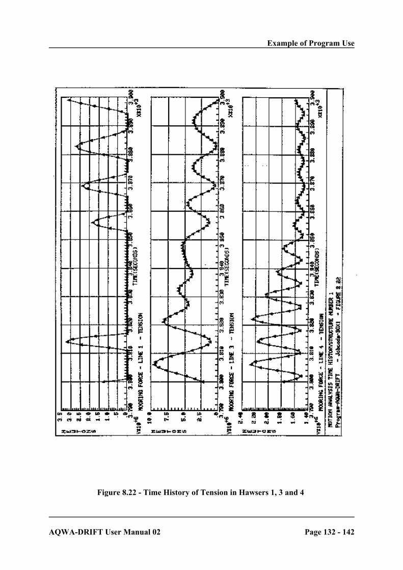
Example of Program Use
AQWA-DRIFT User Manual 02 Page 132 - 142
Figure 8.22 - Time History of Tension in Hawsers 1, 3 and 4

Running the Program
AQWA-DRIFT User Manual 02 Page 133 - 142
CHAPTER 9 - RUNNING THE PROGRAM
To run a program in the AQWA suite, it is necessary to have details of the computer system onwhich the program is loaded. This chapter has sections which are dependent on the computersystem and therefore it lists commands specific to a particular system. It also contains a generaldescription of the most common approach used in running the program.
The following sections describe the use of the program on the following machine:
- PC (MS-DOS) -

Running the Program
AQWA-DRIFT User Manual 02 Page 134 - 142
9.1 Running AQWA-DRIFT on the PC
This chapter is written for the following systems and is NOT applicable to any others.
- MS-DOS PC -
9.1.1 File Naming Convention for AQWA Files
The user must adopt the following convention of naming the files to be used by the AQWAprograms.
Every file name consists of three parts:
C the file prefix a two character lower case string used to identify a particularAQWA program. The file prefixes are as follows:
Program Prefix
AQWA-LINE alAQWA-LIBRIUM abAQWA-FER afAQWA-DRIFT adAQWA-NAUT anAQWA-PLANE apAQWA-WAVE aw
C the run identifer a short name (up to six characters) to identify a particular run. It issuggested that lower case names be used. All the filenamesassociated with the run will contain the same run identifier in theirnames.
C the file extension a three character lower case string to identify the type of the AQWAfile (restart file, hydrodynamics file, etc.). The file extension isseparated from the rest of the filename by a ‘.’ character.
Example
The filename ‘alvlcc.dat’ consists of:
the prefix al (short for AQWA-LINE)the run identifer vlcc (e.g. name of vessel)the extension .dat (input data file)

Running the Program
AQWA-DRIFT User Manual 02 Page 135 - 142
9.1.2 AQWA File Organisation
Every run of an AQWA program involves the use of a number of specially named input, outputand backing files. The following files are used by AQWA-DRIFT:
(.res) file - restart file - backing file
The restart file is used to store all information relating to the structures being analysed. Thisinformation can easily be retrieved on the next run of the analysis sequence, so the input data forthe next run can be considerably simplified. This file is an unformatted binary file.
(.hyd) file - hydrodynamics database file - backing file
This file is used by AQWA-DRIFT and contains a subset of the restart file. It is read only if theALDB option is used.
(.pos) file - positions file - backing file
This file contains the structure positions, for each timestep. It is used by AQWA-PLANE to plottrajectories.
(.plt) file - graphics file - backing file
This file is created and contains positions, velocities, accelerations and all force acting on thestructure at every timestep of the simulation. It is used by AQWA-PLANE to produce timehistory plots.
(.dat) file - input data file
The input data file contains all the AQWA format data decks needed for the current stage ofanalysis (Information from previous stages of analysis may be supplied from the restart file.)The input data file is the only readable input file used in the AQWA suite. It is a normal ASCIItext file.
(.lis) file - output data file - listing file
The output data file receives the main results from a program run. It is a normal ASCII text file.Note that this file contains Fortran carriage control characters - a '1' character in the first columnto designate the top of a new page. This file can be printed on a LaserJet III with the APRINTcommand utility. See the PC User Guide for more information on printer control.
9.1.3 Program Size Requirements
The AQWA programs require an absolute minimum of 4Mb of RAM memory. However, 8Mb(or more) is recommended.

Running the Program
AQWA-DRIFT User Manual 02 Page 136 - 142
9.1.4 Run Commands
When AQWA is installed on a PC an icon is placed on the desktop. The program is usually runby dragging and dropping an AL*.DAT file onto this icon.
However a batch command file is also provided for running all the AQWA programs. This fileshould be located in directory C:\AQWA\UTILS and is named 'AQWAnnn.BAT, where nnn isthe version no. for example 55a. AQWA\UTILS programs can be run from any directoryprovided the C:\AQWA is included in the PATH statement.
To run AQWA-DRIFT version 5.5A, simply type:
AQWA55A DRIFT RUNID
Note: There should be spaces between AQWA, the program name (ie DRIFT), andRUNID where RUNID is the run identifier
If the run identifier is omitted, the program will prompt for a run identifier, which should beentered without any leading or embedded spaces. This name identifies the data files for theanalysis and is also used to name files created by the run.
If the run identifier is (say) TEST, AQWA-LINE will expect and create files with names of theform ALTEST.EXT, where EXT is the file extension. The user must therefore put the input datainto a file named ALTEST.DAT.
For AQWA-DRIFT, the restart and positions files produced by one run will normally need to becopied across to new names for the next run in the sequence.
To illustrate how to run an analysis sequence, the commands needed to run the manual exampleare given below:
AQWA55A LINE BOXM
COPY ALBOXM.RES ADBOXM.RES
AQWA55A DRIFT BOXM

Appendix A
AQWA-DRIFT User Manual 02 Page 137 - 142
APPENDIX A - AQWA-DRIFT PROGRAM OPTIONS
The options listed below may be used when running the program AQWA-DRIFT. They shouldappear on the options card, which follows the job identification card in Administration Deck 0(see Section 6.0).

Appendix A
AQWA-DRIFT User Manual 02 Page 138 - 142
LIST OF OPTIONS FOR USE IN AQWA-DRIFT
ALDB - READ AQWA-LINE DATABASE
Read the hydrodynamics database from the hydrodynamics (.HYD) file created by a previousAQWA-LINE run. This option is used:
I. If the user wishes to modify the hydrodynamic data calculated in a previous AQWA-LINE run, or add/modify nodes and non-diffracting elements, without having to re-runthe AQWA-LINE radiation /diffraction analysis.
II. If the user is setting up an analysis with several structures, and wishes to pick up thehydrodynamic data for one or more structures, calculated in a previous AQWA-LINErun.
Note: Very often, there is data for only one structure in the hydrodynamics file, in which casethe data is associated with Structure 1 in the new run. The RDDB option may also be used if thehydrodynamics file contains more than one structure, provided that all the structures appear, inthe same order, in the new run.
CONV - CONVOLUTION
Instructs AQWA DRIFT or NAUT to use convolution method in radiation force calculation.This is a more rigorous approach to the radiation force calculation in time domain and willenhance the capability of handling non-linear response of structures.
Requests calculation of the full QTF matrix. From version 5.3j onward this option is needed toobtain this.
CRNM - CALCULATE RAOs WITH NO MOORINGS
This option may be used with AQWA-LINE but is more useful with the program AQWA-FER.This option investigates the calculation of RAOs using the values of added mass, wave damping,stiffness and wave forcing specified by the user. The RAOs are then written into the database.
DATA - DATA CHECK ONLY
This option is used to check the data input to the program and provides a means by which theuser may check all input data whilst incurring minium cost of the program run. This option isequivalent to performing the analysis up to the end of the second stage in AQWA-LINE, and upto the end of Stage 4 in AQWA-DRIFT/FER/LIBRIUM/NAUT. If the data proved to be correct,then the program would be restarted at next stage of the analysis by using the RESTART option.
END - This is used to indicate the end of the option list.
FQTF - USE FULL QTF MATRIX

Appendix A
AQWA-DRIFT User Manual 02 Page 139 - 142
This option specifies that the full matrix of difference frequency QTFs is to be used whencalculating slowly varying drift forces.
LAAR - LOCAL ARTICULATION AXIS SYSTEM FOR ARTICULATIONREACTION FORCE OUTPUT (LAA)
This option is used to output articulation reaction force in the local articulation axis system. Thismeans that the moments in unconstrained freedoms, e.g. the hinge axis, will always be zerowithin roundoff.
LSAR - LOCAL STRUCTURAL AXIS SYSTEM (LSA) FORARTICULATION REACTION FORCE OUTPUT
This option is used to output articulation reaction force in the local structural axis system. Thismeans that the direction of the output reaction force will follow the structure.
MCNV - CALCULATE C.I.F. USING ADDED MASS AND DAMPING
From version 5.3K onward the default method for calculation of the Convolution IntegralFunction uses the radiation damping only. This option forces the program to use the previousmethod based on both added mass AND damping.
MRAO - CALCULATE MOTIONS USING RAO’s ONLY
This option instructs AQWA DRIFT to calculate motions using RAOs only. These may bedefined by the user in Deck 7. Note that this option suppresses all motion except that definedby the RAOs. In particular current, wind, drift forces, moorings etc. have no effect on themotions of the structure.
NOBL - NO BLURB. DO NOT PRINT .LIS BANNER PAGE
This option switches off printing of the banner page in the *.LIS file.
NOCP - NO CURRENT PHASE SHIFT
This option switches off the wave phase shift due to a current speed. This is only applicable toversions 5.0C and onwards.
NODL - NO DATA LIST
This option switches off all extended data output in the *.LIS file.
NOST - NO STATISTICS
This option stops the automatic calculation of statistics at the end of each simulation run.Statistical processing can be lengthy for long simulations. This option can be used to reduceprocessing time if statistics are not required.

Appendix A
AQWA-DRIFT User Manual 02 Page 140 - 142
NOWD - NO AUTOMATIC WAVE DRIFT DAMPING CALCULATION
This option stops the automatic calculation of wave drift damping for a floating structure inAQWA DRIFT. When this option is used, the wave drift damping should be defined in deck 9.Otherwise the program will do the calculation. Please note that the wave drift dampingcalculated by the program is only for the floating structure defined in AQWA LINE, dampingfrom risers, etc is not included. The NYWD option stops calculation of wave drift damping foryaw motion only.
NYWD - NO YAW WAVE DRIFT DAMPING
This option suppresses the calculation of wave drift for yaw motion. To prevent the calculationof ALL wave drift damping use the NOWD option.
RDDB - READ DATABASE
Read the hydrodynamics database from the restart (.RES) file created by a previous AQWA-LINE run.
This option is used if the user wishes to modify the hydrodynamic data calculated in a previousAQWA-LINE run, without having to re-run the AQWA-LINE radiation/diffraction analysis.
Note: Normally, this would be done using the option ALDB (see above). The RDDB option isonly needed if the hydrodynamics file from the previous AQWA-LINE run has been accidentallydeleted.
Note that, as the model definition has to be read from the restart file before the hydrodynamicscan be read, there is no possibility to change the model definition, when using this option (useALDB instead).
REST - RESTART
This option is used when the program is being restarted at any stage greater than the first (seeSection 5.2 of the AQWA program manual). A restart card must follow the options list whenthe restart option is used. This card indicates the stage at which the program is to continue andthe stage at which the program is to stop (see Chapter 2).
SDRG - USE SLOW VELOCITY FOR HULL DRAG CALCULATION
This option is used if users wish to use the slow velocity (drift frequency velocity) for the hulldrag calculation, instead of the total velocity (drift frequency velocity + wave frequencyvelocity) which is the default since version 5.0C.
TRAN - TRANSIENT ANALYSIS
This option switches off the slow axis system and stops printout of harmonic analysis at the endof a simulation run. This option should not in general be used. It is only provided as a

Appendix A
AQWA-DRIFT User Manual 02 Page 141 - 142
workaround for DRIFT analysis for both drift and wave frequency motions if it diverges in thetime integration.
TRAO - TRANSIENT RAO MOTION
When this option is used AQWA-DRIFT will recalculate the forces based on the RAOs, whichcan be input by the user in Deck 7. This allows RAOs obtained from (e.g.) Tank tests to be usedwith the CONV option in transient analyses. If the RAOs are not modified this option has littleeffect.
PBIS - PRINT FORCE COMPONENTS AT EACH ITERATION STEP
Prints out positions and forces on each structure at each timestep. The scope of the printout canbe controlled by selections in Deck 18.
PPEL - PRINT PROPERTIES OF EACH ELEMENT
This option allows the user to output complete details of each element used in the bodymodelling. All important details of the body elements are output together with the resultantproperties of the bodies. It is only applicable when running Stage 1 of the analysis.
PRCE - PRINT CARD ECHO FOR DECKS 1 to 5
This option informs the program to output the input received by the program in reading Decks1 to 5. This is the body modelling.

Appendix B
AQWA-DRIFT User Manual 02 Page 142 - 142
APPENDIX B - REFERENCES
1. A Simulation Model For the Dynamic Behaviour of Tankers Moored to Single PointMoorings - B. Molin, G. Bureau, Int. Symposium of Ocean Engineering, (1980)
2. The Influence of Slowly Varying Wave Forces on Mooring Systems - A.E. Loken andO.A. Olsen, OTC 3626 (1979)
3. Second Order Slowly Varying Forces on Vessels in Irregular Waves - J.N. Newman, Int.Symp. on the Dynamics of Marine Vehicles and Structures in Waves, University CollegeLondon, (1974).
4. Prediction of Wind and Current Forces on VLCCs - Oil Companies International MarineForum.
5. Experience in Analysis of SPM Systems - R.C.T. Rainey, D.G.F. Cash and S.G. Withee- OTC 4346 (1982).
6. A Validation of Speed and Frequency Dependence in Seakeeping, Bailey, P.A., Hudson,D.A., Price, W.G. and Temarel, P - Proc. Intl. Shipbuilding Conf. St Petersburg, 1998.
7. The Fifth Annual Fairey Lecture: on the Linear Representation of Fluid Forces andMovements in Unsteady Flow, Bishop, RED, Burcher, R.K., and Price, W.G, Journal ofSound and Vibration, 29 (1): 113-128, 1973