CMPSCI 670: Computer Vision!Deep learning

University of Massachusetts, Amherst November 17, 2014

Instructor: Subhransu Maji

• Homework 4 - grades posted • Homework 5 - due on Wednesday • Project

• Presentations on Dec. 1 and 3 • Each person (or team) will get 7 (or 10) mins to present

- Preliminary results, data analysis, etc

• Final report due on Dec. 13 (hard deadline)

• Next lecture is a guest lecture by: • “Crafting the Perfect Selfie using Computer Vision”

Aditya Khosla, MIT

Administrivia

2

• Shallow vs. deep architectures • Background

• Traditional neural networks • Inspiration from neuroscience

• Stages of CNN architecture • Visualizing CNNs • State-of-the-art results • Packages

Overview

3Many slides are by Rob Fergus and S. Lazebnik

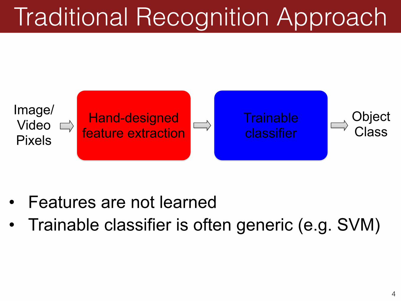
Traditional Recognition Approach

4

Hand-designedfeature extraction

Trainableclassifier

Image/ Video Pixels

• Features are not learned • Trainable classifier is often generic (e.g. SVM)

ObjectClass

• Features are key to recent progress in recognition • Multitude of hand-designed features currently in use

• SIFT, HOG, …………. • Where next? Better classifiers? Or keep building more features?

Traditional Recognition Approach

5

Felzenszwalb, Girshick, McAllester and Ramanan, PAMI 2007

Yan & Huang (Winner of PASCAL 2010 classification competition)

• Learn a feature hierarchy all the way from pixels to classifier • Each layer extracts features from the output of previous layer • Train all layers jointly

What about learning the features?

6

Layer 1 Layer 2 Layer 3 Simple Classifier

Image/ Video Pixels

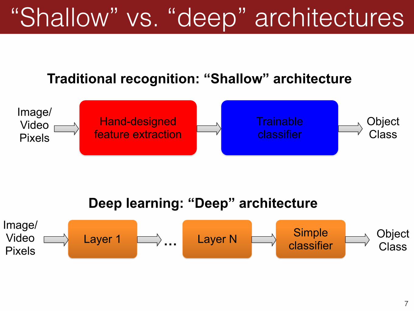
“Shallow” vs. “deep” architectures

7

Hand-designedfeature extraction

Trainableclassifier

Image/ Video Pixels

ObjectClass

Layer 1 Layer N Simple classifier

Object Class

Image/ Video Pixels

Traditional recognition: “Shallow” architecture

Deep learning: “Deep” architecture

…

• Artificial neural network is a group of interconnected nodes • Circles here represent artificial “neurons” • Note the directed arrows (denoting the flow of information)

Artificial neural networks

8

image credit wikipedia

Inspiration: Neuron cells

9http://en.wikipedia.org/wiki/Neuron

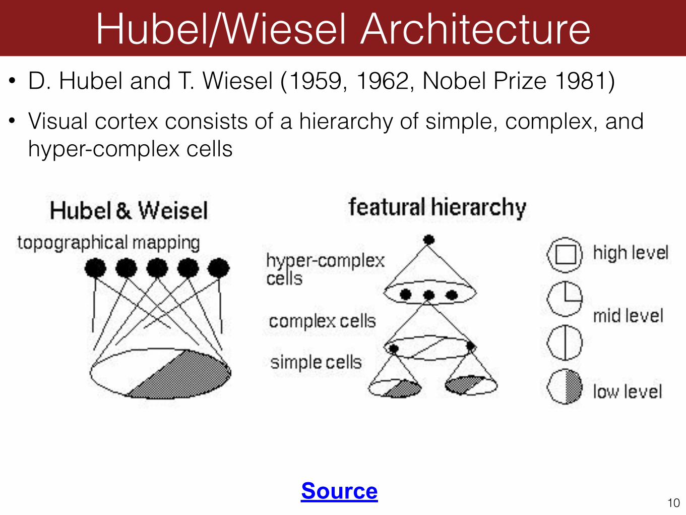
• D. Hubel and T. Wiesel (1959, 1962, Nobel Prize 1981) • Visual cortex consists of a hierarchy of simple, complex, and

hyper-complex cells

Hubel/Wiesel Architecture

10Source

The basic unit of computation

11

x1

x2

xd

w1

w2

w3x3

wd

Sigmoid function:

Input

Weights

.

.

.te

t−+

=11)(σ

Output: σ(w⋅x + b)

“Peceptron”, Frank Rosenblatt 1957

• Without non-linearity, the whole system is linear • Unfortunately, neural network research stagnated for decades

after the publication by Minsky and Papert, 1969, who showed that a perceptron cannot represent the “xor” function

Non-linearity is important

12

• Back-propagate the gradients to match the outputs • Were too impractical till computers became faster

Training ANNs

13

we know the desired output

df(g(x))/dx = (df/dg)(dg/dx)“Chain rule” of gradient

http://page.mi.fu-berlin.de/rojas/neural/chapter/K7.pdf

• In the 1990s, simpler and faster learning methods such as SVMs and boosting were favored over ANNs.

• Why? • Need many layers to learn good features — many parameters

need to be learned • Needs vast amounts of training data (related to the earlier point) • Convergence is slow, get stuck in local minima • Vanishing gradients for deep models

Issues with ANNs

14

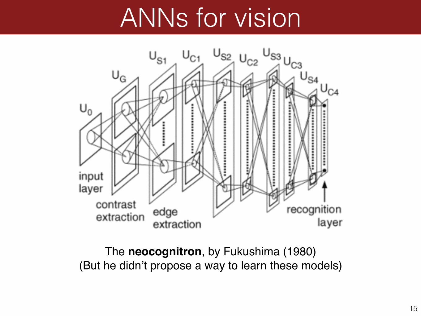
The neocognitron, by Fukushima (1980)!(But he didn’t propose a way to learn these models)

ANNs for vision

15

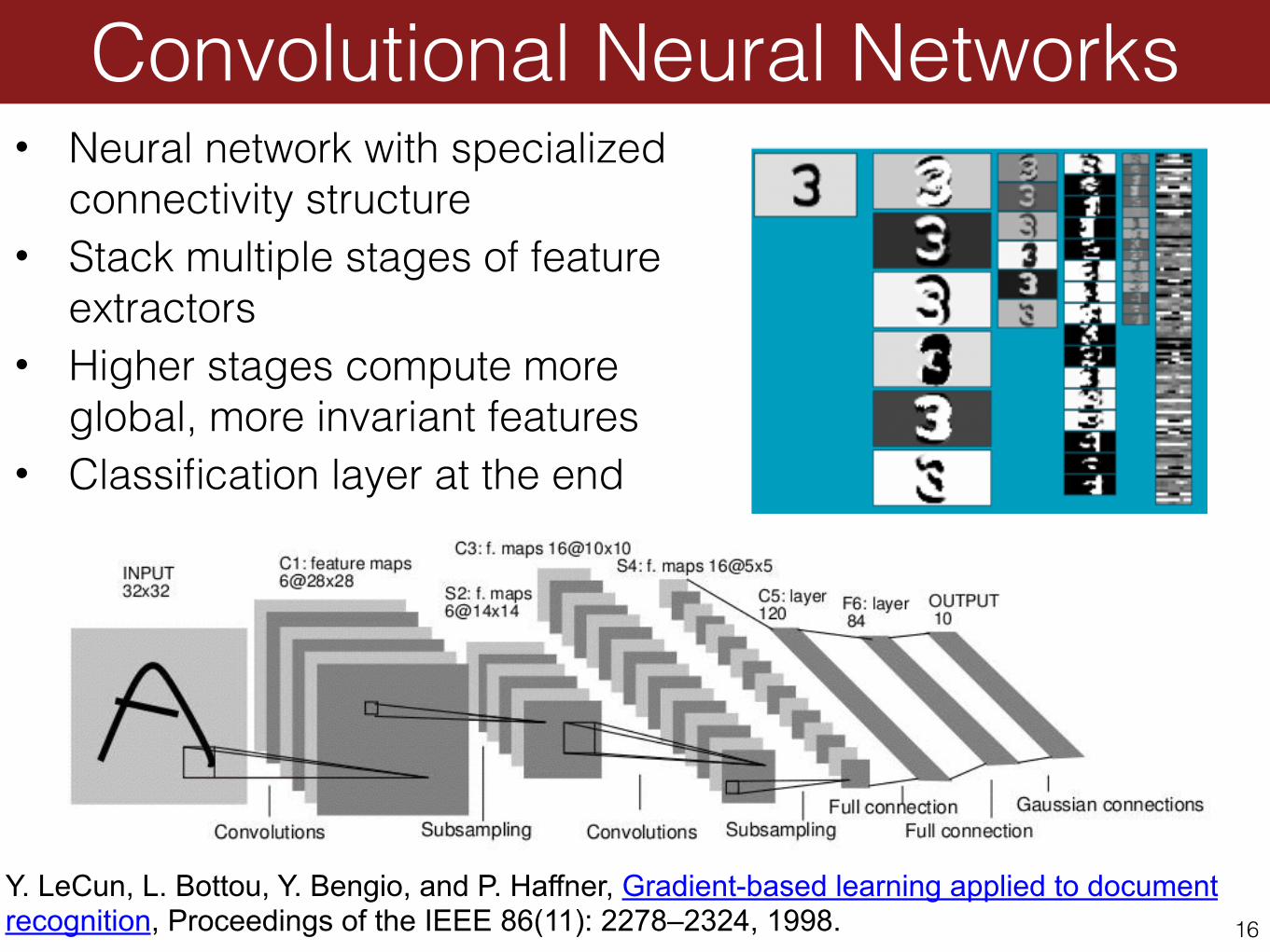
• Neural network with specialized connectivity structure

• Stack multiple stages of feature extractors

• Higher stages compute more global, more invariant features

• Classification layer at the end

Convolutional Neural Networks

16

Y. LeCun, L. Bottou, Y. Bengio, and P. Haffner, Gradient-based learning applied to document recognition, Proceedings of the IEEE 86(11): 2278–2324, 1998.

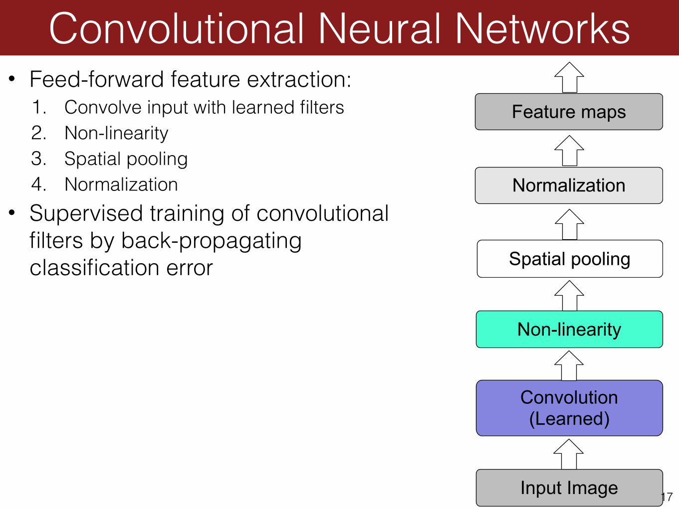
• Feed-forward feature extraction: 1. Convolve input with learned filters 2. Non-linearity 3. Spatial pooling 4. Normalization

• Supervised training of convolutional filters by back-propagating classification error

Input Image

Convolution (Learned)

Non-linearity

Spatial pooling

Normalization

Convolutional Neural Networks

17

Feature maps

• Dependencies are local • Translation invariance • Few parameters (filter weights) • Stride can be greater than 1

(faster, less memory)

1. Convolution

18Input Feature Map

.

.

.

• Per-element (independent) • Options:

• Tanh • Sigmoid: 1/(1+exp(-x)) • Rectified linear unit (ReLU)

- Simplifies backpropagation - Makes learning faster - Avoids saturation issues

à Preferred option

2. Non-Linearity

19

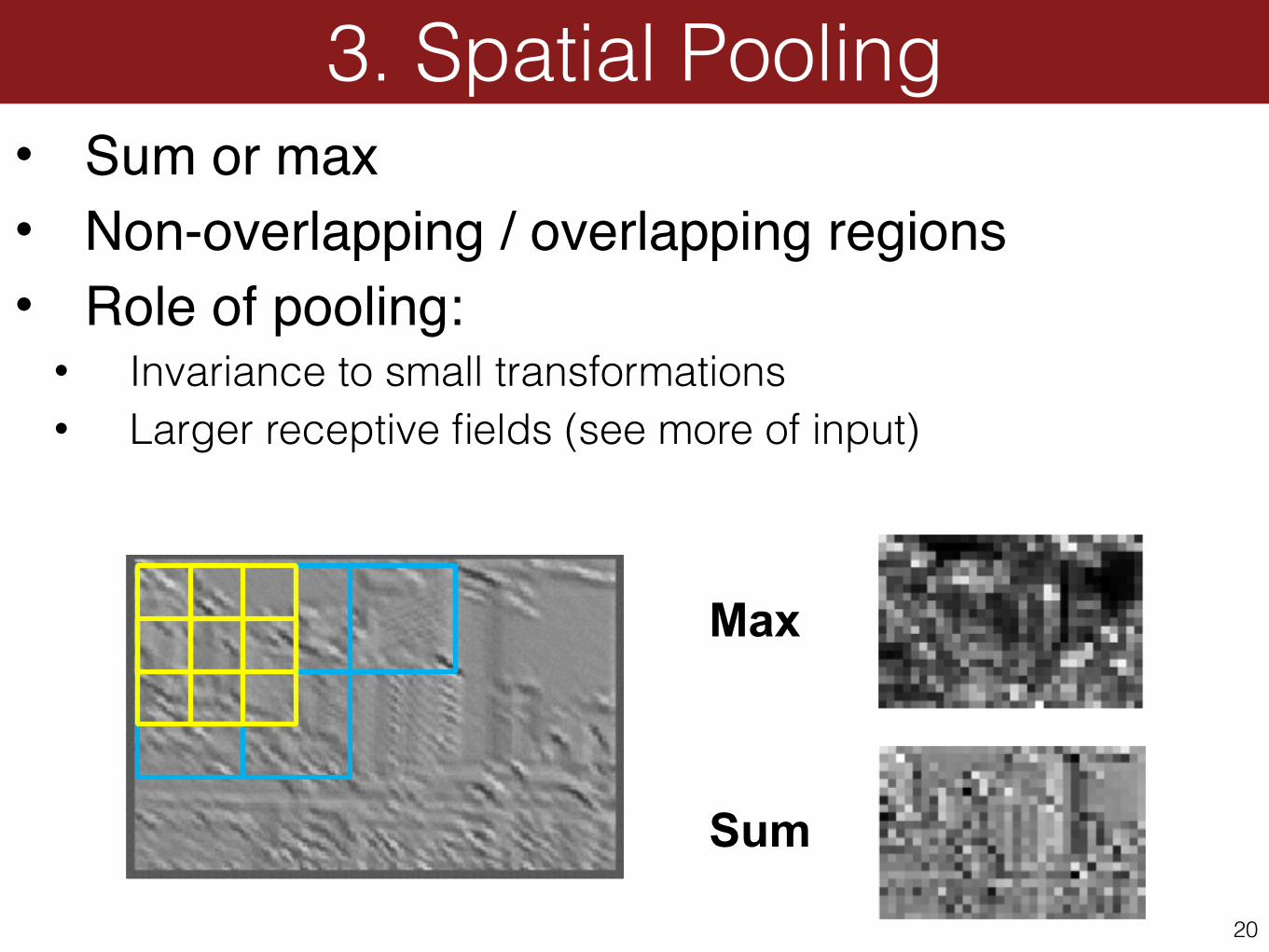
• Sum or max!• Non-overlapping / overlapping regions!• Role of pooling:!

• Invariance to small transformations • Larger receptive fields (see more of input)

3. Spatial Pooling

20

Max

Sum

• Within or across feature maps • Before or after spatial pooling

4. Normalization

21

Feature Maps Feature Maps

After Contrast Normalization

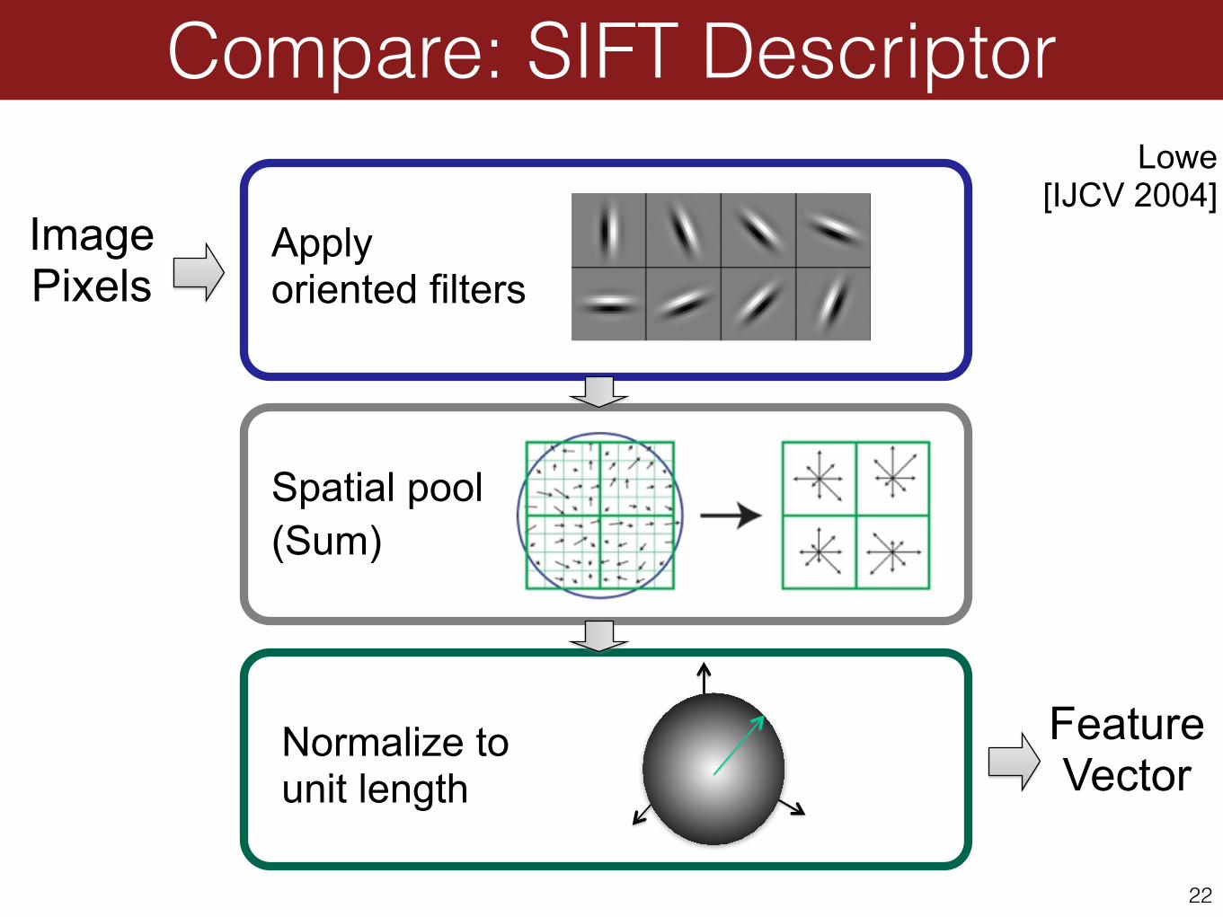
Compare: SIFT Descriptor

22

Applyoriented filters

Spatial pool (Sum)

Normalize to unit length

Feature Vector

Image Pixels

Lowe [IJCV 2004]

• Handwritten text/digits • MNIST (0.17% error [Ciresan et al. 2011]) • Arabic & Chinese [Ciresan et al. 2012]

!

• Simpler recognition benchmarks • CIFAR-10 (9.3% error [Wan et al. 2013]) • Traffic sign recognition

- 0.56% error vs 1.16% for humans [Ciresan et al. 2011] !

• But until recently, less good at more complex datasets • Caltech-101/256 (few training examples)

CNN successes

23

ImageNet Challenge 2012

24

[Deng et al. CVPR 2009]

• 14+ million labeled images, 20k classes • Images gathered from Internet • Human labels via Amazon Turk • The challenge: 1.2 million training

images, 1000 classes

A. Krizhevsky, I. Sutskever, and G. Hinton, ImageNet Classification with Deep Convolutional Neural Networks, NIPS 2012

ImageNet Challenge 2012

25

• Similar framework to LeCun’98 but: • Bigger model (7 hidden layers, 650,000 units, 60,000,000 params) • More data (106 vs. 103 images) • GPU implementation (50x speedup over CPU)

• Trained on two GPUs for a week • Better regularization for training (DropOut)

A. Krizhevsky, I. Sutskever, and G. Hinton, ImageNet Classification with Deep Convolutional Neural Networks, NIPS 2012

Krizhevsky et al. -- 16.4% error (top-5) Next best (SIFT + Fisher vectors) – 26.2% error

ImageNet Challenge 2012

26

Top-

5 er

ror r

ate

%

0

7.5

15

22.5

30

SuperVision ISI Oxford INRIA Amsterdam

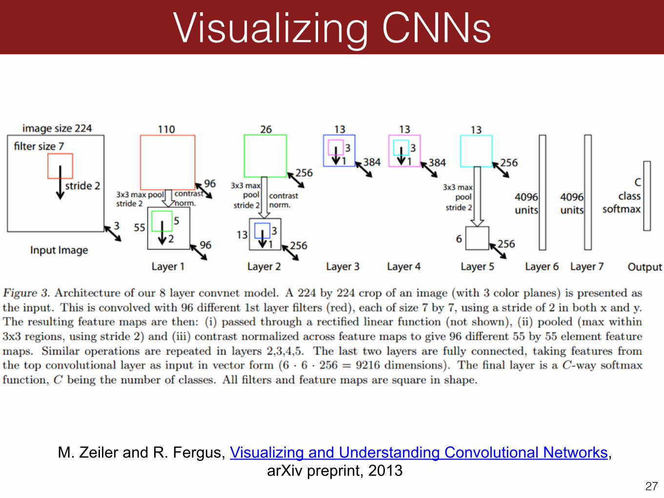
Visualizing CNNs

27

M. Zeiler and R. Fergus, Visualizing and Understanding Convolutional Networks, arXiv preprint, 2013

Layer 1 Filters

28

Similar to the filter banks used for texture recognition

Layer 1: Top-9 Patches

29

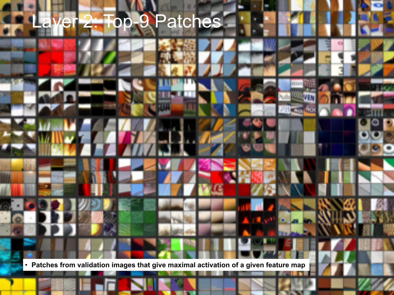
Layer 2: Top-9 Patches

• Patches from validation images that give maximal activation of a given feature map

Layer 2: Top-9 Patches

Layer 3: Top-9 PatchesLayer 3: Top-9 Patches

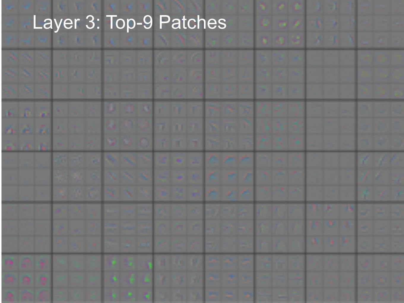
Layer 3: Top-9 Patches

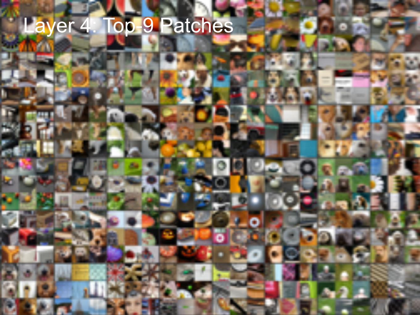
Layer 4: Top-9 Patches

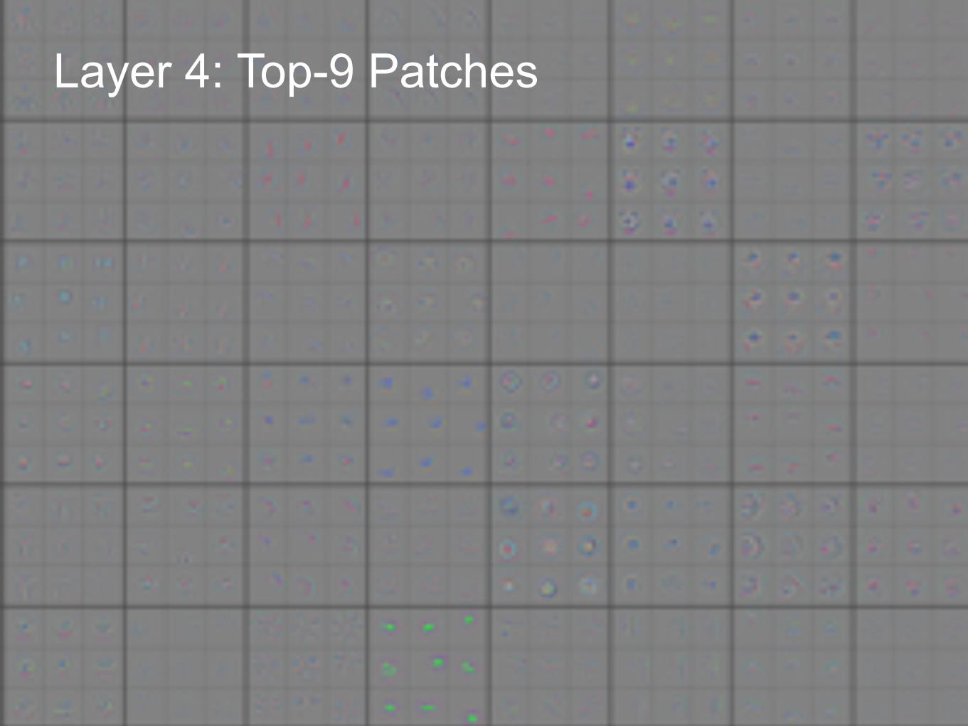
Layer 4: Top-9 Patches

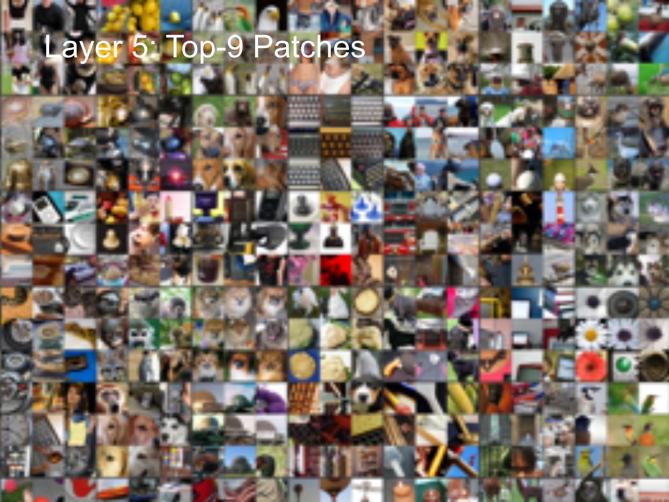
Layer 5: Top-9 Patches

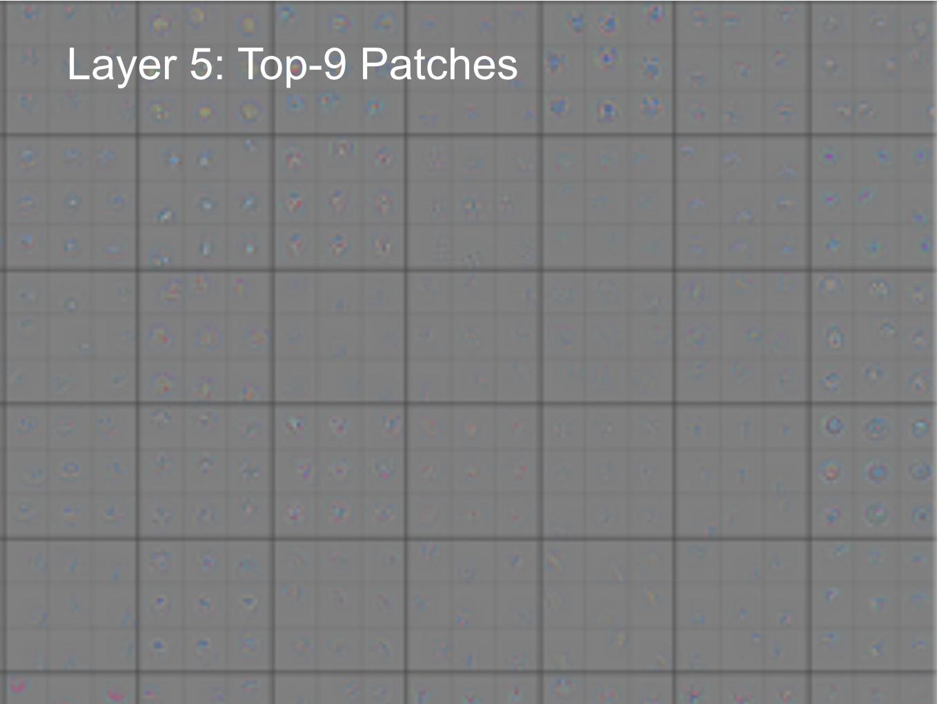
Layer 5: Top-9 Patches

Evolution of Features During Training

38

Evolution of Features During Training

39

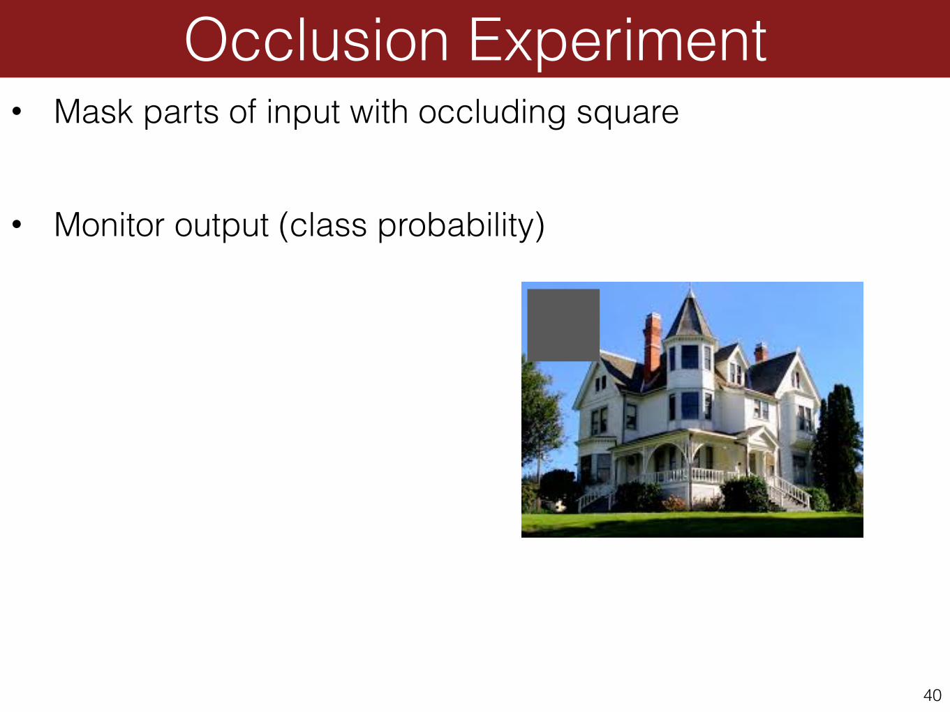
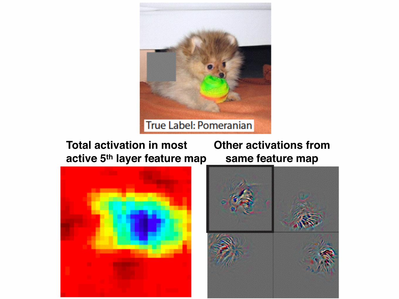
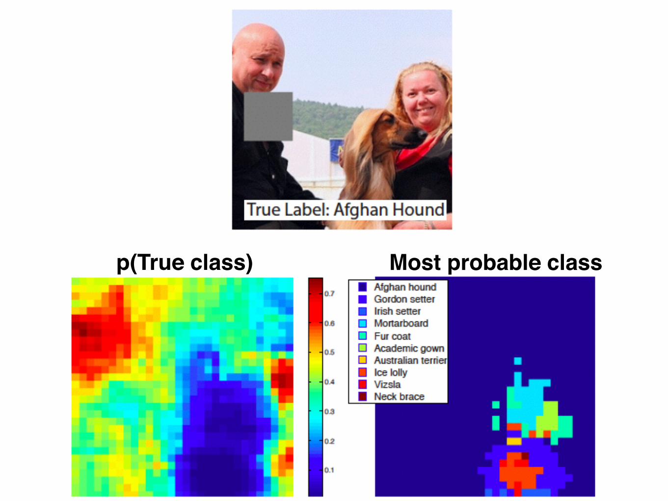
• Mask parts of input with occluding square !

• Monitor output (class probability)

Occlusion Experiment

40

41

Total activation in most active 5th layer feature map

Other activations from same feature map

42

p(True class) Most probable class

43

Total activation in most active 5th layer feature map

Other activations from same feature map

44

p(True class) Most probable class

45

Total activation in most active 5th layer feature map

Other activations from same feature map

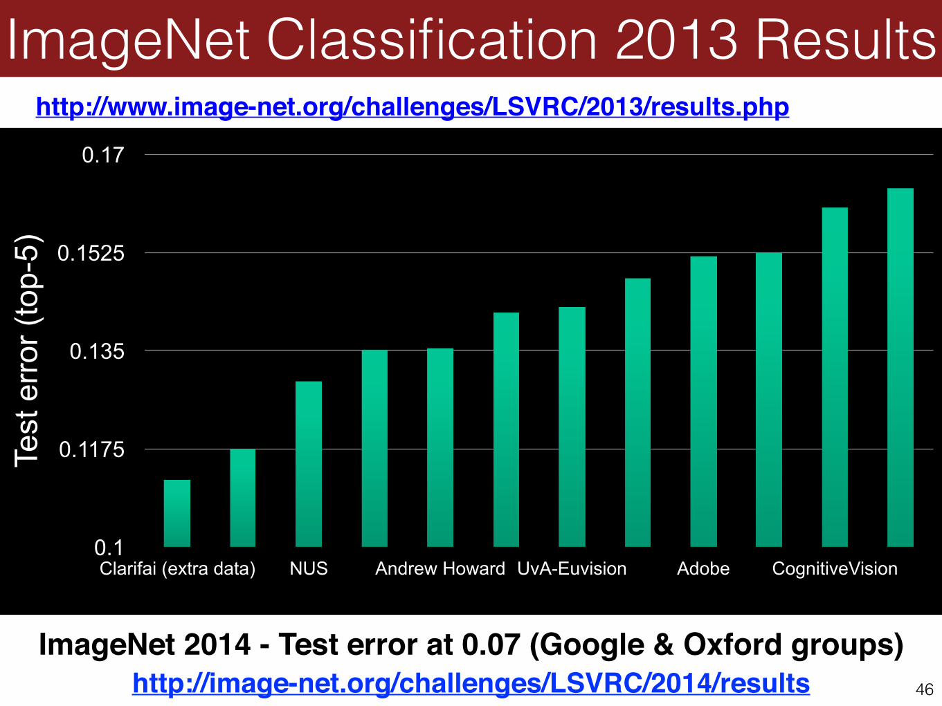
http://www.image-net.org/challenges/LSVRC/2013/results.php

ImageNet Classification 2013 Results

46

Test

err

or (t

op-5

)

0.1

0.1175

0.135

0.1525

0.17

Clarifai (extra data) NUS Andrew Howard UvA-Euvision Adobe CognitiveVision

ImageNet 2014 - Test error at 0.07 (Google & Oxford groups)http://image-net.org/challenges/LSVRC/2014/results

• Take model trained on ImageNet • Take outputs of 6th or 7th layer before or after nonlinearity as

features • Train linear SVMs on these features (like retraining the last

layer of the network) • Optionally back-propagate: fine-tune features and/or

classifier on new dataset

CNNs for small datasets

47

Tapping off features at each Layer

48

Plug features from each layer into linear SVM

Higher layers are better

Results on benchmarks

49

[1] J. Donahue, Y. Jia, O. Vinyals, J. Hoffman, N. Zhang, E. Tzeng, and T. Darrell, DeCAF: A Deep Convolutional Activation Feature for Generic Visual Recognition, arXiv preprint, 2014

[1] SUN 397 dataset (DeCAF)[1] Caltech-101 (30 samples per class)

[2] A. Razavian, H. Azizpour, J. Sullivan, and S. Carlsson, CNN Features off-the-shelf: an Astounding Baseline for Recognition, arXiv preprint, 2014

[2] MIT-67 Indoor Scenes dataset (OverFeat)[1] Caltech-UCSD Birds (DeCAF)

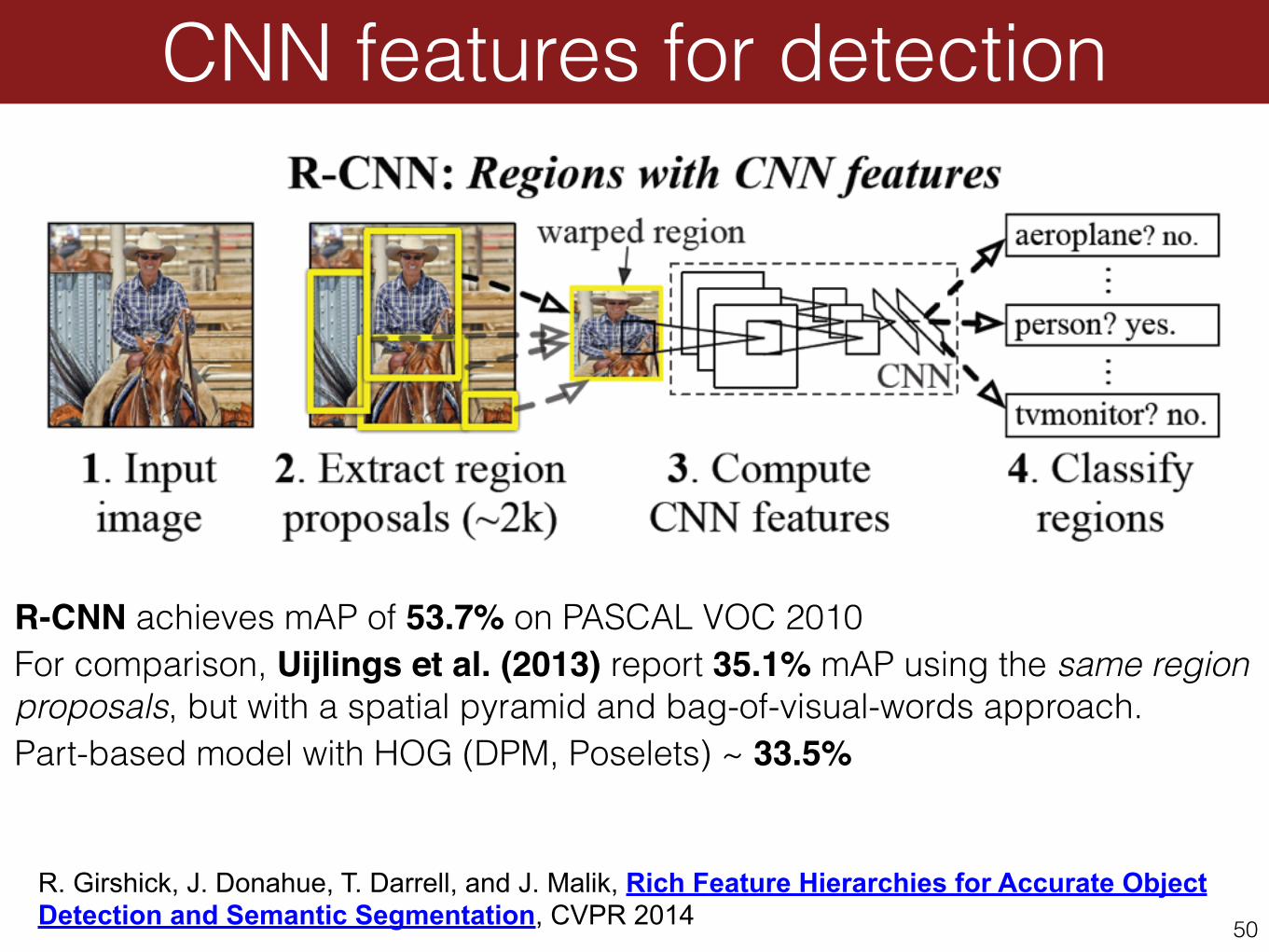
R-CNN achieves mAP of 53.7% on PASCAL VOC 2010 For comparison, Uijlings et al. (2013) report 35.1% mAP using the same region proposals, but with a spatial pyramid and bag-of-visual-words approach. Part-based model with HOG (DPM, Poselets) ~ 33.5%

CNN features for detection

50

R. Girshick, J. Donahue, T. Darrell, and J. Malik, Rich Feature Hierarchies for Accurate Object Detection and Semantic Segmentation, CVPR 2014

CNN features for face verification

51

Y. Taigman, M. Yang, M. Ranzato, L. Wolf, DeepFace: Closing the Gap to Human-Level Performance in Face Verification, CVPR 2014, to appear.

• Cuda-convnet (Alex Krizhevsky, Google) • High speed convolutions on the GPU

• Caffe (Y. Jia, Berkeley) • Replacement of deprecated Decaf • High performance CNNs • Flexible CPU/GPU computations

• Overfeat (NYU) • MatConvNet (Andrea Vedaldi, Oxford)

• An easy to use toolbox for CNNs from MATLAB • Comparable performance/features with Caffe

Open-source CNN software

52