286 IEEE TRANSACTIONS ON BROADCASTING, VOL. 44, NO. 3, SEPTEMBER 1998

nvironmenta

Thomas N. Rubinstein, Senior Member, IEEE

Abstract-To enhance the accuracy of propagation predictions for Broadcasting and Land Mobile applications, a more accurate characterization of clutter loss and of environmental noise has been needed. A series of tests was performed to quantify the environmental RF noise levels associated with various types of ground clutter and to quantify the effects of ground clutter on RF propagation path loss. Tests were performed at 162, 468, and 860 MHz in four different localities in the United States. Each had very different land clutter, as characterized by the LULC categories used in the United States. It was found that the numbers currently in use by industry for clutter loss are, in general, slightly less than the observed values. Both the clutter loss and noise results can be applied to system design.

I. INTRODUCTION

One of the major problems in predicting field strength in the terrestrial point-to-area environment, including both the broadcasting and the land mobile radio services, is the variation in losses due to local land clutter. Most prediction algorithms consider a single number to characterize the loss over an entire area. Given the availability of land clutter databases produced by remote sensing techniques, it is appropriate to characterize the losses due to land clutter on a per-category basis.

The Land Use Land Cover [l] (LULC) database is produced by the United States Department of the Interior, Geological Survey (USGS). The database is based upon remote sensing data which has been categorized according to a scheme described by Anderson et al [2]. While the categories are not ideal for application to radiowave propagation, ths is the only ground clutter database that has complete coverage of the United States. Publisher Item Identifier S 0018-9316(98)08199-2

A series of tests was performed to determine the effects of ground clutter in various LULC categories at the following three frequencies: 162, 460, and 860 MHz. Ground clutter loss was measured at all three frequencies whereas environmental noise was measured at only 162 MHz. The program was performed in the San Diego, Los Angeles, and Atlanta greater metropolitan areas and in Whatcom County in northwestern Washington. This large number of different areas was a deliberate choice to include the broadest possible number of types of terrain.

11. THESURVEY

A. Survey Equipment As shown in Figure 1, an automated survey package, consisting of four calibrated receivers (one for measuring 162 MHz noise plus one receiver per frequency for measuring signal strength), Global Positioning Satellite (GPS) and Differential GPS (DGPS) receivers, an AID converter, and a computer, was used to conduct the survey. Information from the Shadow Loss and LULC category layers was used to automatically disable the taking of data at inappropriate locations. The DGPS equipment was used to keep track of the survey vehicle’s horizontal position. This equipment has a horizontal accuracy of 5 meters or better. The sample size and sub- sample interval were based upon a maximum sampling error of 1 dB, as determined according to a method proposed by Lee [3]. At 162 MHz range, this yields a total sample length of about 53 meters, which can (depending on latitude) be a very substantial fraction of the 3 arc-second horizontal database resolution when run in an East-West direction. Therefore, the runs were made (within the limits of practicality) in a North-South direction. I t was realized that directional effects due to street alignment with the site could result in skewed data; therefore, every reasonable effort was made to

0018-9316/9&$10.00 0 1998 IEEE

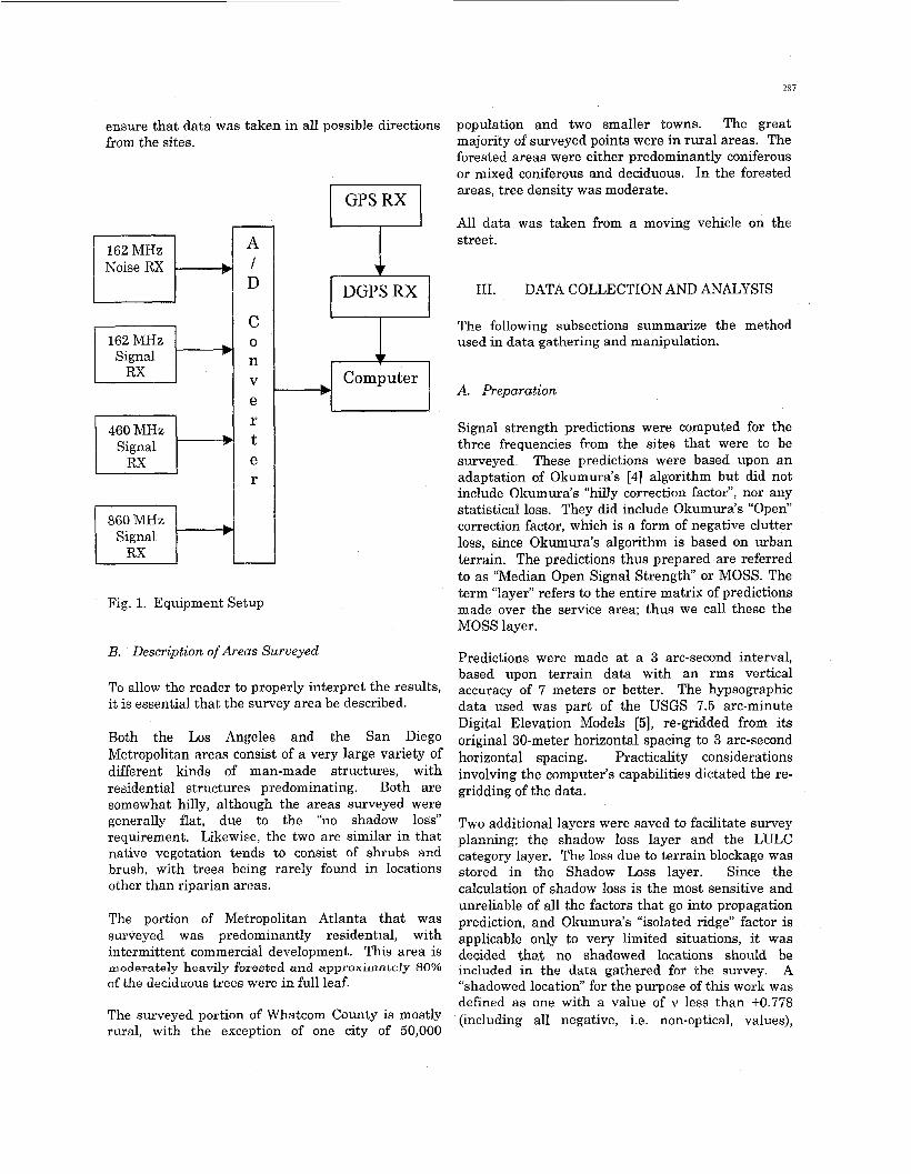
ensure that data was; taken in all possible directions from the sites.

Noise RX

162 MHz Signal

Signal

Signal

A 1 B

C

n

e

t

0

V

r

e r

DGPS RX 9 4-l Comp U t e r

Fig. 1. Equipment Setup

B. Description of Areas Surveyed

To allow the reader to properly interpret the results, it is essential that the survey area be described.

Both the Los Angeles and the San Diego Metropolitan areas consist of a very large variety of different kinds of man-made structures, with residential structures predominating. Both are somewhat hilly, although the areas surveyed were generally flat, due to the “no shadow loss” requirement. Likewieie, the two are similar in that native vegetation tends to consist of shrubs and brush, with trees being rarely found in locations other than riparian areas.

The portion of Metropolitan Atlanta that was surveyed was predominantly residential, with intermittent commercial development. This area is moderately heavily forested and approximately 80% of the deciduous trees were in full leaf.

The surveyed portion of Whatcom County is mostly rural, with the exception of one city of 50,000

287

population and two smaller towns. The great majority of surveyed points were in rural areas. The forested areas were either predominantly coniferous or mixed coniferous and deciduous. In the forested areas, tree density was moderate.

All data was taken from a moving vehicle on the street.

111. DATA COLLECTION AND ANALYSIS

The following subsections summarize the method used in data gathering and manipulation.

A. Preparation

Signal strength predictions were computed for the t h e e frequencies from the sites that were to be surveyed. These predictions were based upon an adaptation of Okumura’s [4] algorithm but did not include Okumura’s “hilly correction factor”, nor any statistical loss. They did include Okumura’s “Open” correction factor, which is a form of negative clutter loss, since Okumura’s algorithm is based on urban terrain. The predictions thus prepared are referred to as “Median Open Signal Strength” or MOSS. The term “layer” refers to the entire matrix of predictions made over the service area; thus we call these the MOSS layer.

Predictions were made at a 3 arc-second interval, based upon terrain data with an rms vertical accuracy of 7 meters or better. The hypsographic data used was part of the USGS 7.5 arc-minute Digital Elevation Models [5], re-gridded from its original 30-meter horizontal spacing to 3 arc-second horizontal spacing. Practicality considerations involving the computer’s capabilities dictated the re- gridding of the data.

Two additional layers were saved to facilitate survey planning: the shadow loss layer and the LULC category layer. The loss due to terrain blockage was stored in the Shadow Loss layer. Since the calculation of shadow loss is the most sensitive and unreliable of all the factors that go into propagation prediction, and Okumura’s “isolated ridge” factor is applicable only to very limited situations, it was decided that no shadowed locations should be included in the data gathered for the survey. A “shadowed location” for the purpose of this work was defined as one with a value of v less than +0.778 (including all negative, i.e. non-optical, values),

288

where v is the dimensionless diffraction parameter used in the Fresnel integrals [6].

Similarly, there is no need to survey locations without a corresponding LULC category, so such locations were eliminated from the survey.

B. Data Reduction

The following procedure was followed to analyze the data:

The data for various days’ runs for a given locality was combined The signal strength data (but not the noise data) was subtracted from the predicted MOSS layer data a t each point of predictiodmeasurement. Data was separated into files corresponding to the various combinations of frequency band I type of measurement (signal difference or noise) I and LULC category. Each new file was sorted by signal difference value or noise value, as appropriate. Summary files, boxplots, and histograms were created.

IV. RESULTS

The following Tables summarize the survey results.

A. Environmental Noise

The data for the noise measurements was taken in 4 locations: San Diego, Los Angeles, Whatcom County WA, and Atlanta. Because of the similarity of the terrain and development of the two areas, the data for San Diego and Los Angeles were combined. Table I summarizes the noise measurement data.

Before constructing this table, it was found that the Atlanta noise data contained an unusually Barge number of points with extremely strong signals. This was tracked-down to the operator who performed the survey not having been adequately instructed on monitoring for intermodulation and what to do about it. Therefore, data indicating extremely strong signals (> -70 dBm a t the receiver’s antenna terminal) in Atlanta was removed. Since there was no data at all in the range -100 to -70 dBm, it was felt that this was a safe thing to do because such a gap in signal statistics would be

unlikely to exist in the real world. This accounts for the larger number of samples in Table 1 for the Noise data than for the Signal Strength Difference data in the table to follow. I t is recognized, however, that some of the data indicating signals weaker than -70 dBm could have received undetected contamination, resulting in noise statistics showing stronger than actual values.

The per-category results for the various ]locations were compared and it was found that they did not track between areas. However, an interesting trend emerged: The larger the metro area, the higher the noise level, as shown in Table 1, where the mean for the data a t each location is shown.

83. Signal Strength Difference (SSD)

The data for the signal strength difference measurements was, like the environmental noise measurements, taken in 4 locations: San Diego, Los Angeles, Whatcom County WA, and Atlanta. And again, because of the similarity of the terrain and development of the two areas, the data for San Diego and Los Angeles were combined.

The Whatcom County signal strength difference data appears to be bad for both the 162 MHz and 460 MHz bands, as it does not track at all with the other areas. The 860 MHz SSD data as well as the 162 MHz noise data track well with the other areas. It is, therefore, surmised that there were problems with the test setup involving the 162 MHz and 460 MHz test receivers. That data was not considered further.

After the Atlanta survey was completed, it was learned that the system being used as a signal source for testing in the 460 MHz band was a simulcast system. This tainted all of the 460 MHz Atlanta data, which should, therefore, be disregarded.

Additionally, the data taken in the Los Angeles area in Categories 21-24 appears to have been corrupted by database problems. The area in question was shadowed, but the database did not show it. Therefore, those data should be disregarded.

The data summary is presented in Table 11.

289

- Descrirhion

Table I Summary of Noise Measurements

162 MHz

# Samdes Noise Category

ATL

11 12 13

dB Re1 to kToB

14 15

SCA __

16 17

NWW

21 22

- Reciidential

Industrial - Commercial & Services

23 24

31

1981 293 1199 10 349 1

32 33

Industrial & Comm’l Complexes Mixed Urban or Built-up Land

41 42 43

19 55 29

52 53 54

Other Urban or Build-up Land

CrolpPand & Pasture Orchards, Groves, Vineyards, Nurseries, Ornamental Horticulture Confined Feeding Operations Othler Agricultural Land

61 62

75

143 34

275 423 34

110 7 36

76

13.64 13.23 12.72

I I I I I I

Transitional Areas (barren) 56 I I 16 I 16.78 I I 12.36

SCA = Southern California; NWW = Northwest Washington; ATL = Atlanta

290

Table PI Summary of Signal Strength Difference Measurements

V. DISCUSSION

A. Discussion of Observations

In a number of the categories, a very substantial number of samples was taken. In others, few samples were taken. Yet another group of categories (51, 71-74, SI+) was not sampled at all. Differences in application of the noise versus the SSD data are discussed below.

1) Noise: All noise data acquired appears, on the surface, to be reasonable. There were, however, some LULC Categories for which the data was so sparse that it is not reasonable to expect that it

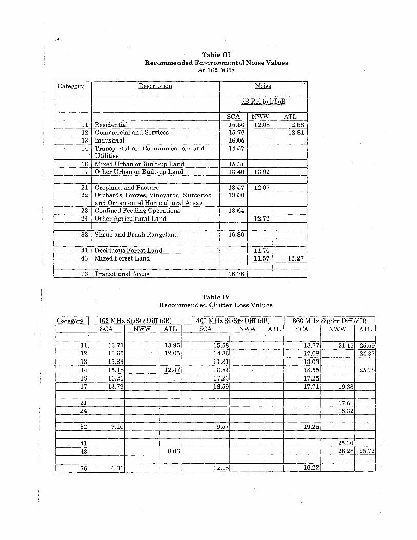
contains a representative sample. Therefore, the data for Categories 31, 33, 52, 53, 54, 61, 62, and 75 was not considered further. Additionally, there were several categories where the data taken in a given area was insufficient to make a recommendation for that particular area. The minimum number of samples for inclusion in the table was set a t 30, remembering that n 2 30 is often cited in the calculation of the large sample confidence interval. As stated in Walpole and Myers [7], “the justification lies only in the presumption that with a sample as large as 30, s will be very close to the true CT and thus the Central Limit Theorem prevails. Since it is clear that the noise level within a given category varies with the morphology of the area (i.e. Large City, Medium City, Rural), the following table is split into such values. See Table I11 for recommended values.

291

2) Signal Strength Difference: In LULC categories 31, 33, 52, 53, 54, 61, 62, and 75, there was so little data that ,the potential for error is great. Since the confidence interval for any given confidence level is proportional to oldN, a larger M narrows the confidence interval. Additionally, there were several categories where the data taken in a given area was insufficient to make a recommendation for that particular area. The minimum number of samples for inclusion in the table was set at 30. (Of the data that remains, all appears to be reasonable with the exception of the value for Category 43 in a Medium City at 460 MHz, which represents a large gain. Since it is clear that the signal strength difference within a given category varies with thie morphology of the area (i.e. Large City, Medium City, Rural), the following table is split into such values. See Table IV for recommended values.

B. Potential Sources of Error

Even when every effort was made to eliminate or reduce error sources to a minimum, error will inevitably creep in. The following have been identified as potential error sources:

1) Error Sources Applicable to Both Noise and Signal Difference Measurement:

to eliminate grids that were not properly categorized. However, it is perfectly conceivable that one or more of the operators may have failed to invalidate some mis- categorized grids.

e Registration errors Both the terrain data and the LULC data were originally sampled on a Universal Transverse Mercator (UTM) grid. Since the UTM crossings do not precisely register with the LatitudeLongitude crossings used by the prediction algorithm, some errors are bound to have occurred. Speed variation The automated test setup depends on a constant speed to make its measurements. If speed is sufficiently reduced after the beginning of sampling, the software will automatically invalidate the sample. However, small reductions or increases in speed will not trigger this. Despite the fact that the drivers were instructed to maintain as constant a speed as practical, the sampling interval between subsamples may vary.

e Routes: non-representative subcategory samples Each category within the LULC scheme consists of many types of structures or ground cover. For example, Category 1 1 “Residential” includes single family dwellings, apartment buildings, barracks, shacks, etc. To be truly representative of these sub-categories, a survey should include the proportional amount of samples for each sub-category. Unfortunately, this is completely beyond the bounds of practicality.

e Routes: under-representation of narrow streets Because of time constraints, it is not practical to include a significant number of samples on narrow local streets. They are, therefore, underrepresented in the data.

0 Mobile antenna pattern distortion Because of “real estate” limitations on the vehicle roof, it was not

0

Stability of Calibration m i l e measurements have possible to space the antennas so that they were outside

therefore, be expected. Multipath and running the routes in all directions from the site should partially mitigate this problem-

shown the receivers in use to be quite stable, there is the ofone-another’s near field. Some panem distortion can, possibility of drift in calibration.

a Mis-categorization ~h~ LULC survey data in of the areas surveyed was done as much as 20 years prior to the survey. Inevitably, some of the categories will have changed. A facility was provided for the operator

292

Table HIP Recommended Environmental Noise Values

At 162 MHz

41 Deciduous Forest Land 11.70 43 Mixed Forest Land 11.57 12.27

I 1 I I

76 I Transitional Areas 1 16.78 1

Table IV Recommended Clutter Loss Values

293

2) Error Sources Applicable Only to Signal Difference Measurement:

0 Lack of adherence to Okumura Model When writing a computer program, it is not possible to perfectly model a n algorithm that is defined by curves. Further, assumptions had to be made as to what Okumura would do if the limits of the model, were exceeded.

e Database errors The database used has an rms vertical error’ of 7 meters maximum. On rare occasions, this can cause a shadow that exists to be missed by the program, resulting in the measurement of a point that should not be measured. The program includes a facility for manually invalidating such samples, but inevitably the operator may miss some.

0 Routes: North - South To maximize the number of samples taken, the routes are run North-South as much as possible. This could cause the set of samples for a given category to be non-representative because of street alignment with the site. Because of that possibility, routes are put in as many different directions from the! site as possible. Base antenna pattern While both vertical and horizontal patterns were included in the predictions with which the measured data was compared, pattern distortion could not be adequately considered because of limitations in both the pattern distortion calculation program and limitations in the site information available to us. Indeed, thle pattern distortion program does not calculate pattern distortion in the vertical plane at all.

3) Error Sources: Applicable only to Noise Measurement:

e Intermodulation on noise monitoring channel Occasional intermodulation interference was observed on noise monitoring channels. When it was observed, the current sample was invalidated and a different noise- monitoring channel was found. However, it is safe to assume that at least some intermodulation samples remain in the data.

The survey program has identified clutter loss numbers for application to mobile radio systems at the following frequency ranges: 162, 460, and 860 MHz. It has also identified noise values for 162 MHz. It is recommended that the noise values in Table 111 and the clutter loss values in Table IV be used in the design of broadcasting and land mobile radio systems. In areas of the world other than the United States, it is recommended that similar studies be performed to ascertain the corresponding values for the land clutter categories used in those areas.

VII. ACKNOWLEDGMENT

The author would like to thank Mr. Carl B. “Bernie” Olson for his support and encouragement, Mssrs. Dennis M. Allen and Warren D. “Dave” Atherton for their assistance with and modification of the survey hardware and software, Mssrs. Dennis L. Mills, Christopher R. Zona, Wallace M. “Skip” Osteyee Jr., and George €3. Neville for their assistance with the survey, Dr. Garry C. Hess for his helpful suggestions on how to best treat the statistics, and Mr. Allen L. Davidson for doing a preliminary review.

REFERENCES

[l] Land Use and Land Cover Digital Data from 1:250,000 and l : l O O , 000-Scale Maps: Data Users Guide 4, U.S. Geological Survey, Reston, Virginia, 1990.

[Z] Anderson, James R. e t al, A Land Use and Land Cover Classification System for Use with Remote Sensor Data, Geological Survey Professional Paper 964, U.S. Geological Survey, Alexandria VA, 1976.

power of a mobile radio signal”, IEEE Trans Veh Tech, 34(1), Feb 1985, pp 22-27.

[4] Okumura, Yoshihisa e t al, “Field strength and its variability in VHF and UHF land-mobile radio service”, Rev Electrical Comm Lab, Vol 16, 9-10, Sept-Oct 1968, pp 825-873.

[5] Digital Elevation Models: Data Users Guide 5, U.S. Geological Survey, Reston, Virginia, 1990.

163 Jordan, Edward C., Electromagnetic Waves and Radiating Systems, Prentice-Hall, 1950, 5 15.06.

E73 Walpole, Ronald E. & Raymond H. Myers, Probability and Statistics for Engineers and Scientists, 4 t h Ed., Macmillan, 1989, 57.4.

[3] Lee, William C.Y., “Estimate of local average

VI. CONCLUSIONS AND RECOMMENDATIONS