
Clustering - University of Pittsburgh
52
Clustering
Transcript of Clustering - University of Pittsburgh

Clustering
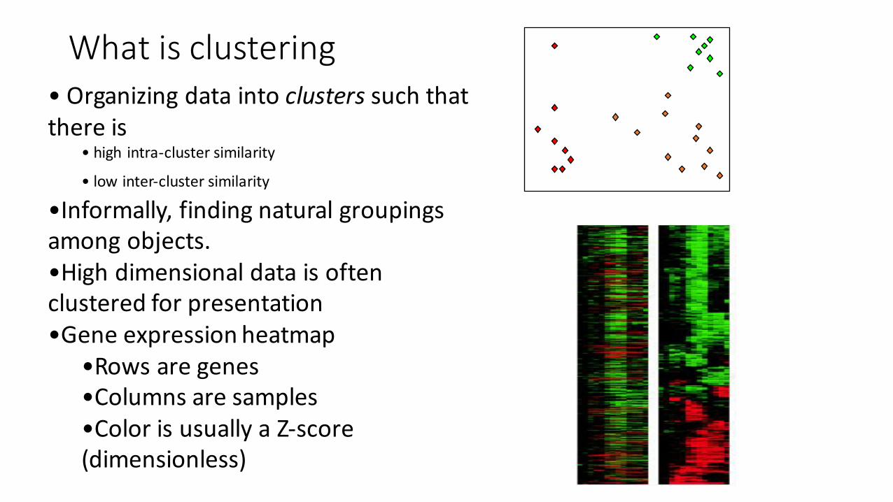
What is clustering• Organizing data into clusters such that there is
• high intra-‐cluster similarity
• low inter-‐cluster similarity
•Informally, finding natural groupings among objects.•High dimensional data is often clustered for presentation•Gene expression heatmap
•Rows are genes•Columns are samples •Color is usually a Z-‐score (dimensionless)

How significant is the clustering
Random 1 –randomized by rows.
Random 2 –randomized by columns.
Random 3 –randomized by both rows and columns.

Gene clustering: biological interpretation• Given a number of biologically distinct samples each gene has a specific patter of expression• Gene expression is controlled by some upstream pathways that are shared across genes• Examples: genes whose products are needed in stoichiometric quantities are highly correlated• Ribosome• Proteasome• ATP-‐synthase

Purpose of clustering• Clustering across genes• Define functionally related gene classes• Can be used to infer functions of unknown genes
• Clustering across samples• Define groups of related samples• Example: infer the number of molecularly distinct cancer subtypes
• Both• Visualization• Dimensionality reduction:
• Instead of saying genes X1,X2,X3… were up-‐regulated in samples Y1, Y2, Y3,…• Glycolysis genes were highly upregulated in the subtype A

Types of clustering• Connectivity/bottom up/hierarchical clustering• Centroid based: k-‐means• Model based: mixture of Gaussians• Dimensionality reduction techniques• PC, NMF

Hierarchical clustering
• Probably the most popular clustering algorithm in gene expression• First presented in this context by Eisen in 1998
• Agglomerative (bottom-‐up)• Algorithm:
1. Initialize: each item a cluster2. Iterate:
• select two most similar clusters• merge them
3. Halt: when there is only one cluster left
. Cluster analysis and display of genome-‐wide expression patterns. PNAS

Hierarchical clustering Calculate the Distance Matrix-‐euclidean distance
Chip2Chip1Gene
1.0-2.0A
-0.5-1.5B
0.251.0C
CBA
3.091.580.00A
2.610.001.58B
0.002.613.09C

Hierarchical clustering
DCBA
4.743.091.580.00A
5.002.610.001.58B
2.700.002.613.09C
0.002.705.004.74D
CBDA

Hierarchical clustering Average Linkage-‐update new distance with the average
DCAB
4.812.850.00AB
2.700.002.85C
0.002.704.81D
CDBA

Hierarchical clustering
CDAB
3.830.00AB
0.003.83CD
DCBA

Details:• Need a measure of similarity among two data vectors• Euclidian distance• 1-‐Correlation (raw and absolute value), rank(Spearman) correlation
• Also need a measure of similarity across clusters with multiple data vectors—how to we update our distance matrix when clusters are formed• Average linkage -‐ midpoint. • Single linkage – smallest distance. • Complete linkage -‐ largest distance.
• Very fast• No need to specify number of clusters• Important: final dendrogram is rotated arbitrarily: rotation freedom can be used to highlight or conceal different aspects of the data

Outlier
One potential use of a dendrogram is to detect outliersOne potential use of a dendrogram is to detect outliers
The single isolated branch is suggestive of a data point that is very different to all others

Example I Cell Cycle
• Cyclins are a family of proteins that control the progression of cells through the cell cycle by activating cyclin-‐dependent kinase (Cdk) enzymes• Experimental design: use a microarray experiment to find out how genes are regulated with cell-‐cycle genome wide• Spellman et al that was published in Mol. Biol. Cell 9, 3273-‐3297 (1998).

Example: cell -‐cycle Methods
• DNA microarrays of the yeast genome• Synchronization: cells must be in the same phase of the cell cycle• α factor.• Elutriation – size based. • Cdc15 – heat mutation.
• Manipulation-‐induction of cyclins• cln3p, clb2p deletion.
• Data from a previously published study (Cho et al. 1998) • Control sample: asynchronous cultures.
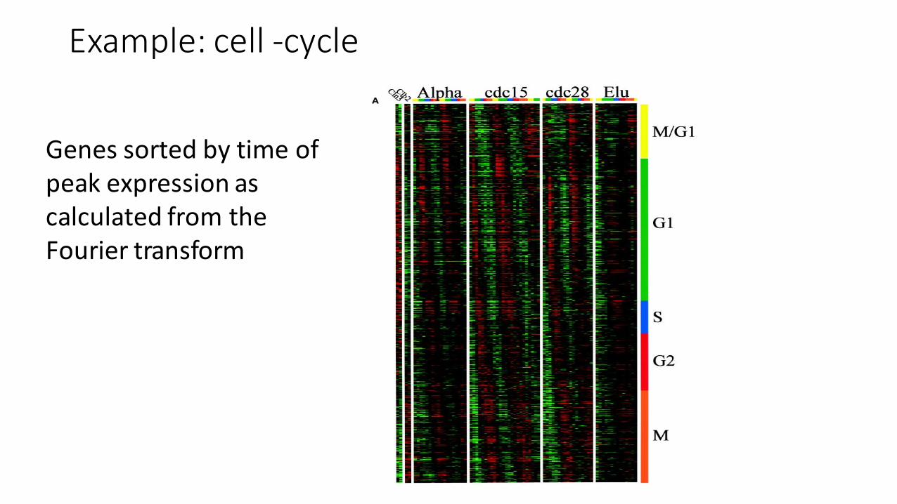
Example: cell -‐cycle
Genes sorted by time of peak expression as calculated from the Fourier transform

Example: cell -‐cycle Clustering
Genes sorted by their hierarchical cluster relationships-‐-‐ similarity of expression across the measurements:

Example: cell -‐cycle• Cell-‐cycle timing was correlated with function for many genes with no obvious cell-‐cycle activity • “The “MET” cluster was completely unexpected. It contains 10 genes involved in the biosynthesis of methionine.”

Example: cell -‐cycle
• Genes in each cluster share DNA binding motifs• Extract upstream promoter sequence for each genes• Use Gibbs sampling (covered later) to identify overrepresented sequence for each cluster
• MCM1:T-T-A-C-C-N-A-A-T-T-N-G-G-T-A-A
• SFF: G-T-M-A-A-C-A-A
• New motif:
T-T-W-C-C-Y-A-A-W-N-N-G-G-W-A-A-W-W-N-R-T-A-A-A-Y-A-A

K-‐means clustering K-‐means clustering • Partition clustering• Nonhierarchical, each instance is placed in exactly one of K non-‐overlapping clusters.
• Since the output is only one set of clusters the user has to specify the desired number of clusters K.
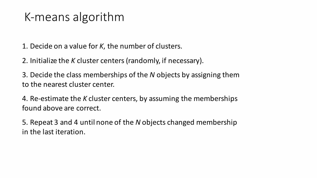
1. Decide on a value for K, the number of clusters.
2. Initialize the K cluster centers (randomly, if necessary).
3. Decide the class memberships of the N objects by assigning them to the nearest cluster center.
4. Re-‐estimate the K cluster centers, by assuming the memberships found above are correct.
5. Repeat 3 and 4 until none of the N objects changed membership in the last iteration.
K-‐means algorithm

22
K-‐means example, step 1
k1
k2
k3
X
Y
Pick 3 initialclustercenters(randomly)
23
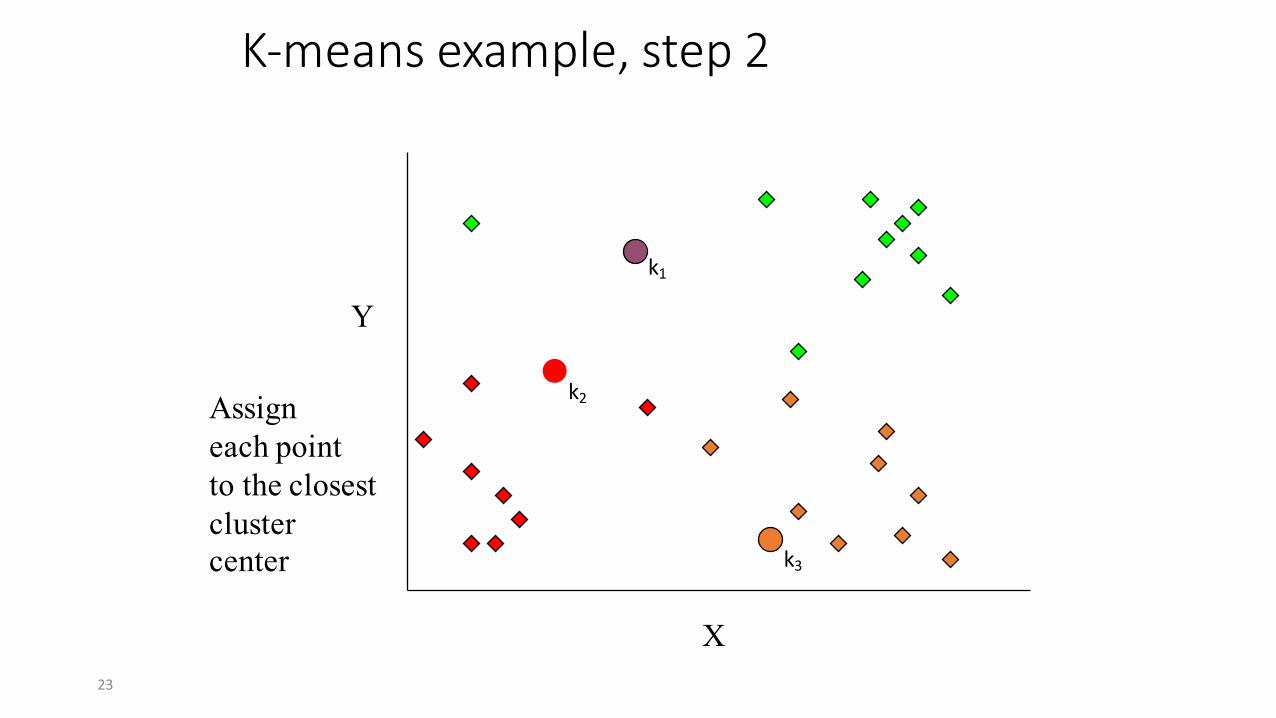
K-‐means example, step 2
k1
k2
k3
X
Y
Assigneach pointto the closestclustercenter

24
K-‐means example, step 3
X
Y
Moveeach cluster centerto the meanof each cluster
k1
k2
k2
k1
k3
k3
25
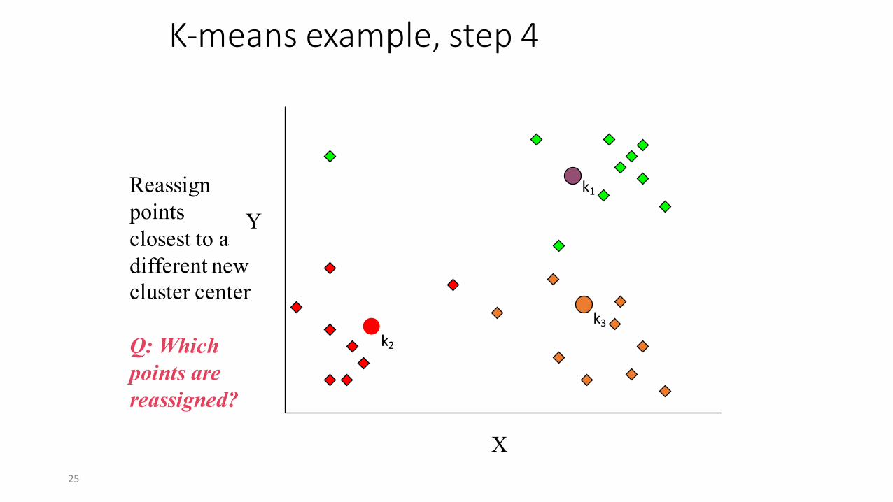
K-‐means example, step 4
X
YReassignpoints closest to a different new cluster center
Q: Which points are reassigned?
k1
k2k3

26
K-‐means example, step 4 …
X
Yk1
k3k2

27
K-‐means example, step 4b
X
Yre-compute cluster means
k1
k3k2

28
K-‐means example, step 5
X
Y
move cluster centers to cluster means
k2
k1
k3
0
1
2
3
4
5
0 1 2 3 4 5
expression in condition 1
expression in condition 2
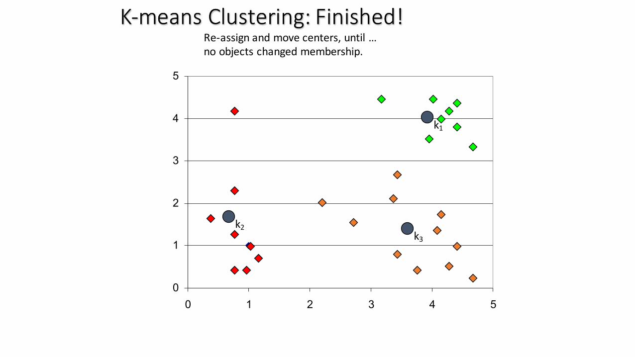
K-‐means Clustering: Finished!K-‐means Clustering: Finished!Re-‐assign and move centers, until …no objects changed membership.
k1
k2k3
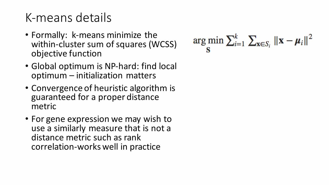
K-‐means details• Formally: k-‐means minimize the within-‐cluster sum of squares (WCSS) objective function• Global optimum is NP-‐hard: find local optimum – initialization matters• Convergence of heuristic algorithm is guaranteed for a proper distance metric• For gene expression we may wish to use a similarly measure that is not a distance metric such as rank correlation-‐works well in practice

Optimal number of clusters• No right answer• Depends on assumptions/prior expectation about data distribution• What is the variance in a cluster• What shape should the clusters be?

10
1 2 3 4 5 6 7 8 9 10
123456789
One option: How does the objective function change as we increase k

1 2 3 4 5 6 7 8 9 10
When k = 1, the objective function is 873.0

1 2 3 4 5 6 7 8 9 10
When k = 2, the objective function is 173.1

1 2 3 4 5 6 7 8 9 10
When k = 3, the objective function is 133.6

0.00E+00
1.00E+02
2.00E+02
3.00E+02
4.00E+02
5.00E+02
6.00E+02
7.00E+02
8.00E+02
9.00E+02
1.00E+03
1 2 3 4 5 6
We can plot the objective function values for k equals 1 to 6…
The abrupt change at k = 2, is highly suggestive of two clusters in the data. This technique for determining the number of clusters is known as “knee finding” or “elbow finding”.
Note that the results are not always as clear cut as in this toy example
k
Objective Functio
n

Model based clustering• K-‐means assumes that the clusters are equal area “spheres”: we assume that assignment to the nearest cluster is correct.• We can define a more general framework but we have to make more model assumptions• Popular model based technique is gaussian mixture models

• Decide the number of clusters, K• Initialize parameters (randomly)
• E-‐step: assign probabilistic membership to all input samples
• M-‐step: re-‐estimate parameters based on probabilistic membership• Repeat until change in parameters is smaller than a threshold
Gaussian Mixture Models
p(x) =kX
i=0
⇡iN(x|µk,⌃k)

Number of parameters• We can specify relative flexibility for
• We specify if clusters can have different covariance, if the diagonal entries are equal and if the non-‐diagonal entries are non-‐zero• "EII": spherical, equal volume • "VII": spherical, unequal volume • "EEI": diagonal, equal volume and shape • "VEI": diagonal, varying volume, equal shape• "EVI": diagonal, equal volume, varying shape • "VVI": diagonal, varying volume and shape• "EEE": ellipsoidal, equal volume, shape, and orientation • "EEV": ellipsoidal, equal volume and equal shape • "VEV": ellipsoidal, equal shape• "VVV": ellipsoidal, varying volume, shape, and orientation
• What about the number of clusters• We can compute the likelihood based on the model• Increasing the number of parameters always increases the likelihood of the data we need to define a parameter penalty

Example
• x = the observed data;• θ = the parameters of the model;• n = the number of data points in xx, the number of observations, or equivalently, the sample size;
• k = the number of free parameters to be estimated. If the model under consideration is a linear regression,
• L= the maximized value of the likelihood function of the model MM, i.e. L̂ =p(x|θ̂ ,M) where θ̂ are the parameter values that maximize the likelihood function.
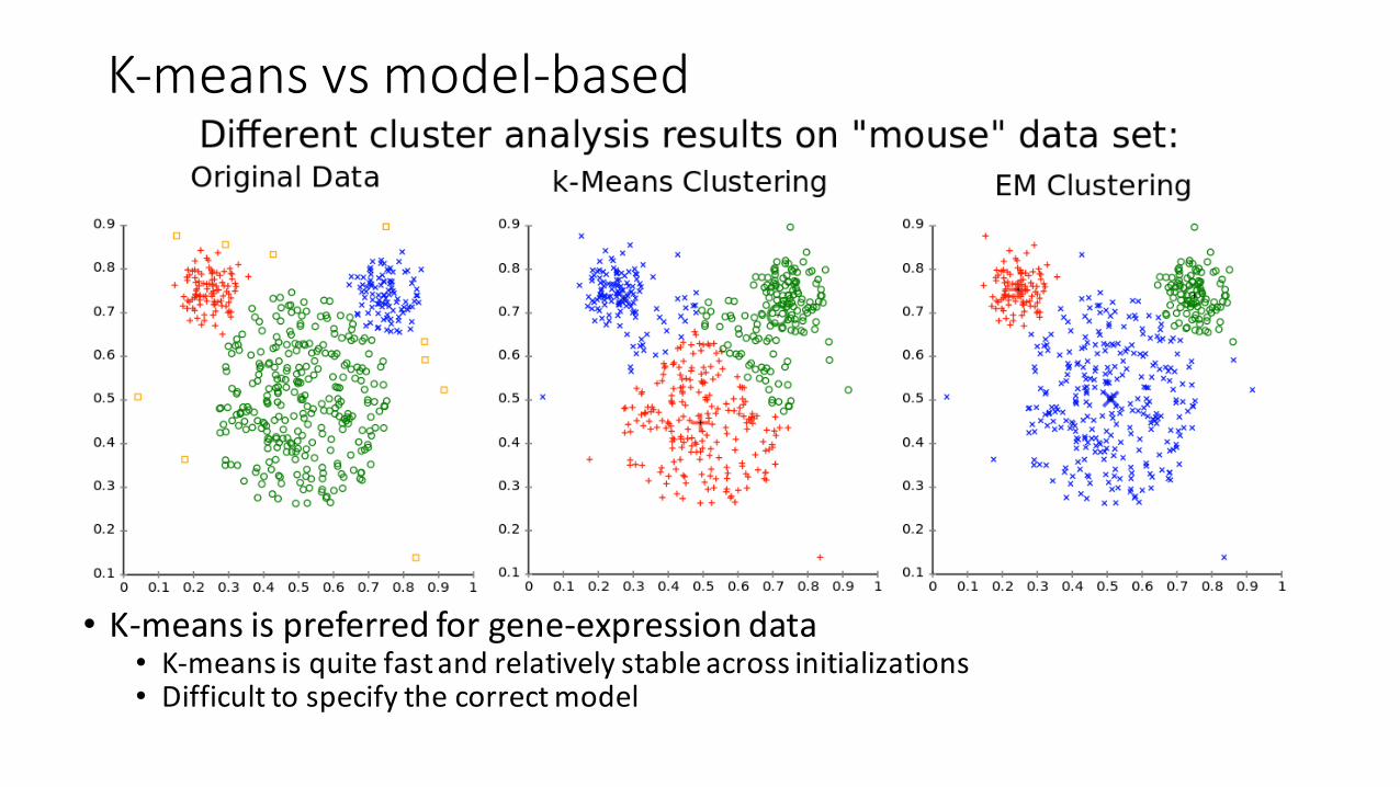
K-‐means vs model-‐based
• K-‐means is preferred for gene-‐expression data• K-‐means is quite fast and relatively stable across initializations• Difficult to specify the correct model

PCA for gene expression• Given a gene-‐by-‐sample matrix M we decompose (row a centered and scaled) M as UDVT
• We don’t usually care about total expression level and the dynamic range which may be dependent on tehcnical factors
• U, V orthonormal• D diagonal-‐elements are eigenvalues
• Variance explained• Columns of are
• principle components• Eigengenes/metagenes• recurrent patters of gene expression
• Columns of U are the “loadings” is the correlation between it and the component • Truncating U,V,D to the first k dimensions gives the best k-‐rank approximation of U

PCA for gene expression: example• Breast cancer samples
• Estrogen receptor (ER) status: ER+, red; ER-‐ , black).
• (b) PCA identifies the two directions (PC1 and PC2) along which the data have the largest spread. (c) Samples plotted in one dimension using their projections onto the first principal component (PC1) for ER+, ER-‐and all samples separately.
• (e) PCA biplot with samples plotted in two dimensions using their projections onto the first two principal components, and two genes plotted using their weights for the components (green points).
• (f) Samples colored according to ERBB2 status (blue, ERBB2+; brown, ERBB2-‐ ; green, unknown).
What is principal component analysis?Nature Biotech

PCA applied to cell cycle data
Singular value decomposition for genome-‐wide expression data processing and modeling. PNAS
GeneExpression=UDVT

Relationship with original data

Other decomposition techniques• Non negative matrix factorization• A= WH (A,W,H are non-‐negative)• Many computational methods
• Cost function |A-‐WH|• Squared error-‐aka Frobenius norm• Kullback–Leibler divergence to positive matrices
• Optimization procedure• Most use stochastic initialization and the results don’t always converge to the same answer
• H defined a meta-‐gene space: similar to eigengenes• Classification can be done in the meta-‐gene space
Metagenes and molecular pattern discovery using matrix factorization PNAS

Example: classifying leukemia• acute myelogenousleukemia (AML)• acute lymphoblastic leukemia (ALL),• Hierarchical clustering did no correctly recover the subtypes

Determining k by cluster stability• Consensus matrix C : what fraction of times two data points ended up in the same cluster• NMF with different initializations• For deterministic methods we can sue subsampling
• Cophenetic correlation• 1-‐C gives us a distance• We cluster based on this distance to get a clustering tree• Copheneticcorrelation tells us how well the resulting tree distance reproduces the initial 1-‐C

NMF vs PCA• NMF operates in the original non-‐negative measurement space• Highly expressed genes matter more
• Positivity constraint is advantageous: positive correlation among genes is more likely to be biologically meaningful
• NMF may more accurately capture the data generating process
• A= WH : Toy Biological interpretation• Assume k=2• We have 2 transcription factors that activate gene signatures W1 and W2
• H represents the activity of each factor in each sample
• TF effects are additiveReducing microarray data via nonnegative matrix factorization for visualization and clustering analysis

Example: identifying subclasses of HCC• Hepatocellular carcinoma: highly heterogeneous liver cancer• Study design: identify reliable molecular sub-‐classes that are consistent across different datasets representing different patient cohorts• Integrative transcriptome analysis reveals common molecular subclasses of human hepatocellular carcinoma. Cancer Research• Subclass Mapping: Identifying Common Subtypes in Independent Disease Data Sets PLoS One
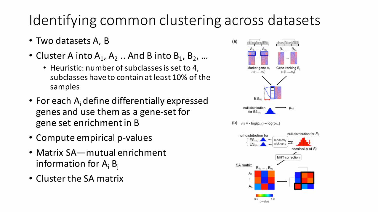
Identifying common clustering across datasets• Two datasets A, B• Cluster A into A1, A2 .. And B into B1, B2, …
• Heuristic: number of subclasses is set to 4, subclasses have to contain at least 10% of the samples
• For each Ai define differentially expressed genes and use them as a gene-‐set for gene set enrichment in B• Compute empirical p-‐values• Matrix SA—mutual enrichment information for Ai Bj• Cluster the SA matrix

• Use a consensus of hierarchical, k-‐means, and NMF clustering (clustering on meta-‐genes)• Identify 3 common clusters with consistent clinical phenotype, molecular markers and pathway activation
Application to HCC