Clustering of Gaze During Dynamic Scene Viewing is Predictedby Motion

Parag K. Mital • Tim J. Smith •

Robin L. Hill • John M. Henderson

Received: 23 April 2010 / Accepted: 5 October 2010

� Springer Science+Business Media, LLC 2010

Abstract Where does one attend when viewing dynamic

scenes? Research into the factors influencing gaze location

during static scene viewing have reported that low-level

visual features contribute very little to gaze location espe-

cially when opposed by high-level factors such as viewing

task. However, the inclusion of transient features such as

motion in dynamic scenes may result in a greater influence of

visual features on gaze allocation and coordination of gaze

across viewers. In the present study, we investigated the

contribution of low- to mid-level visual features to gaze

location during free-viewing of a large dataset of videos

ranging in content and length. Signal detection analysis on

visual features and Gaussian Mixture Models for clustering

gaze was used to identify the contribution of visual features

to gaze location. The results show that mid-level visual

features including corners and orientations can distinguish

between actual gaze locations and a randomly sampled

baseline. However, temporal features such as flicker, motion,

and their respective contrasts were the most predictive of

gaze location. Additionally, moments in which all viewers’

gaze tightly clustered in the same location could be predicted

by motion. Motion and mid-level visual features may influ-

ence gaze allocation in dynamic scenes, but it is currently

unclear whether this influence is involuntary or due to cor-

relations with higher order factors such as scene semantics.

Keywords Eye movements � Dynamic scenes � Features �Visual attention � Clustering

Introduction

Eye movements are a real-time index of visual attention and

cognition. Due to processing and visual acuity limitations,

our eyes shift (saccade) up to five times every second so that

the light from the area of the scene we are interested in is

projected onto the most sensitive part of the retina (the fovea).

Perception of visual detail and encoding in memory only

occurs for the information at the center of attention when the

eyes stabilize on a point in space (fixations) [1–3]. The factors

that influence how we distribute our attention while viewing

static visual arrays and scenes have received a lot of attention

(see [3, 4] for reviews), but very little is known about how we

attend to more realistic dynamic scenes.

The earliest investigations of eye movement behavior

during scene viewing [5, 6] portrayed two main ways in

which visual attention can be controlled: involuntary cap-

ture of attention by external, stimulus features such as

luminance and color (exogenous) and voluntary allocation

of attention according to internal, cognitive factors that

focus attention on cognitively relevant features of the

All eye-movement data and visualization tools can be obtained from:

http://thediemproject.wordpress.com.

P. K. Mital (&)

Department of Computing Goldsmiths, University of London,

London, UK

e-mail: pkmital@gmail.com

T. J. Smith

Department of Psychological Sciences, Birkbeck,

University of London, London, UK

R. L. Hill

Department of Psychology, School of Philosophy,

Psychology and Language Sciences, University

of Edinburgh, Edinburgh, UK

J. M. Henderson

Department of Psychology and McCausland Center for Brain

Imaging, University of South Carolina, Columbia, SC, USA

e-mail: john.henderson@sc.edu

123

Cogn Comput

DOI 10.1007/s12559-010-9074-z

world (endogenous). Being involuntary, exogenous control

should be consistent across all viewers leading to a high

degree of coordination in where and when multiple viewers

attend given the same stimuli. By comparison, endogenous

control should result in less coordination of attention across

individuals as the internal cognitive states of the individual

and their relation to the current stimuli are less predictable.

Previous evidence of the contribution of exogenous and

endogenous factors to gaze control during scene viewing is

mixed. When participants free-view still images presented

on a computer screen, low-level image properties in static

scenes differ significantly at fixation compared to control

locations [7–15]. Specifically, high-spatial frequency edge

information is higher at fixation than at control locations

[7, 8, 11, 12, 15], as is local contrast (the standard deviation

of luminance at fixation) [8, 9, 13–15], texture [16], and

mid-level visual features composed of multiple superim-

posed orientations, including corners [17, 18].

The discovery of distinct visual features around fixation

led to the development of several computational models of

attentional allocation in scenes e.g. [19–25]. These models

are all predicated on the assumption that conspicuous visual

features ‘‘pop-out’’ and involuntarily capture attention [26].

This assumption is founded on evidence from classic visual

search paradigms using simple visual arrays e.g. [27] which

have shown that visual features such as color, motion, and

orientation can be used to guide attention (see [4] for

review). Computational models of attention allocation

combine multiple basic visual features at multiple spatial

scales in order to produce a saliency map: an image distri-

bution predicting the conspicuity of specific locations and

their likelihood of attracting attention [19, 26, 28]. The

widely used computational model of visual saliency devel-

oped by Itti and Koch [19, 28] has been shown to predict

fixation locations better than chance under some conditions

[21, 28]. For example, medium salience objects are fixated

earlier than low-salience objects during memorization [29].

However, subsequent investigations have shown that the

model’s predictions are correlational in nature and not

causal. Visual saliency correlates with objects [30] and is

biased toward the screen center in the same way fixations are

[15]. Visual salience explains very little of the variance of

fixation locations when this correlation is removed by

instructing viewers to search for a particular target [8, 29,

31–34]. The visual features used to compute visual saliency

are also used by our early visual system to identify higher

order features such as objects which are the intended target

of attention [30, 35]. During interactive tasks, endogenous

control becomes even more pronounced as gaze is tightly

linked to the completion of goals such as steering a car,

filling a kettle, or walking down the street [36–39].

However, it could be argued that previous investigations

into the relationship between visual saliency and gaze in

static scenes have been biased against saliency due to the

omission of the visual feature shown to most robustly capture

attention: motion. The unexpected onset of a new object and

the associated motion transients are the only visual features

shown to robustly capture visual attention without endoge-

nous pre-setting (i.e. the instruction to search for a specific

feature such as ‘‘red’’) [40–42]. Given that onsets do not

normally occur in static scenes, no exogenous control should

be predicted. Only with the artificial addition of onsets into a

static scene is exogenous control observed resulting in

immediate fixation of the new object [43–45]. It is not nec-

essarily the new object that captures attention but the motion

transients associated with its appearance (see [46] for

review). If an onset occurs during a saccade, saccadic sup-

pression masks the motion transients caused by the object’s

appearance and no oculomotor capture occurs [43–45]. The

sudden appearance of new objects and the associated motion

transients are the only visual features that are known to

exogenously control attention irrespective of endogenous

factors [40], and neither feature occurs in static scenes.

However, both occur in abundance in dynamic scenes.

The recent addition of dynamic visual features such as

motion and difference-over-time (flicker) to computational

models of visual saliency has resulted in a significant

increase in their ability to predict human gaze location in

dynamic scenes compared to models which only utilize

static features, e.g. color, intensity, and edges [47–53].

Motion and flicker are the strongest independent predictors

of gaze location in dynamic scenes, and their independent

contributions are as high, if not higher, than the weighted

combination of all features in a model of visual salience [48,

50]. However, most previous investigations of dynamic

scene viewing have heavily biased the viewing conditions

toward exogenous control. Viewers have been biased

toward motion by being instructed to ‘‘follow the main

actors or actions’’ [48–51] and by using very short video

clips (1–3 s) edited together into an unrelated sequence that

minimizes the contribution of endogenous factors such as

memory and ongoing event comprehension [48, 49]. Carmi

and Itti [48, 49] showed that exogenous control was highest

immediately following a cut to a new, semantically unre-

lated scene and decreased monotonically over the next

2.5 s. Studies that have used longer video sequences have

also been potentially confounded by the impact of cuts as

the videos used were ‘‘found’’ footage gathered from tele-

vision, film, or home movies and analysis was performed

across the entire video [47, 50–52]. Without isolating cuts,

it is unclear whether the contribution of visual features to

fixation location is due to exogenous control within an

ongoing dynamic event or due to the sudden, abrupt pre-

sentation of a new scene following a cut.

As well as, predicting higher visual feature values at

fixation compared to control locations, exogenous control

Cogn Comput

123

of attention may also predict clustering of the gaze of

multiple viewers in the same location. If the contrast

between visual features at a specific scene region and the

whole scene causes the region to ‘‘pop-out’’, then viewers

should be involuntarily drawn to the same location at the

same time. This would create a high degree of consistency

in where viewers attend in a dynamic scene. Such clus-

tering of gaze during dynamic scene viewing has been

reported in several studies [48, 54–62] and is believed to be

an integral part of film viewing (see [63] for a review). For

example, Goldstein et al. [54] showed 20 adults six long

clips from Hollywood movies and found that for more than

half of the viewing time the distribution of fixations from

all viewers occupied less than 12% of the screen area. This

Attentional Synchrony effect is observed for feature films

[48, 54–58, 60–63], television [59], and videos of real-

world scenes [53, 60, 64].

In static scenes, fixations from multiple viewers have been

shown to cluster in specific scene regions but not at the same

time [12]. The only exception is a bias of fixations toward the

screen center [15, 65], which has also been observed in

dynamic scenes [52]. A systematic analysis of the factors

contributing to this central bias in dynamic scenes suggests

that it is due to a bias in positioning focal, foreground objects

at screen center and a tendency for viewers to saccade to the

screen center immediately following scene onset (or fol-

lowing a cut) [66]. Both of these factors explain why a

sudden increase in clustering has been observed immediately

following cuts [48, 53]. The central bias also presents

problems for analyses of visual features at fixation as sal-

iency has also been shown to have a slight but significant

center bias in natural scenes [15, 67]. Therefore, the higher

visual features reported at fixation may be an incidental

consequence of the tendency to cluster gaze at screen center

immediately following cuts. Given confounds of central

tendency and cuts in previous studies, it is currently unclear

what contribution visual features make to gaze clustering

during dynamic scene viewing. The only way to subtract the

effect of central tendency from the contribution of visual

features to gaze location is to (1) present dynamic scenes for

longer to give the eyes time to explore the scene; and (2)

compare the visual features at fixation to control locations

which share the same central tendency (e.g. fixations sam-

pled from a different time point during the same movie [15,

65]). These methods were adopted in the present study.

The Dynamic Scene Study

What are the contributions of low and mid-level static and

dynamic visual features to attention during dynamic scene

viewing? Do visual features contribute more when gaze of

multiple viewers is tightly clustered and do such moments

occur throughout a dynamic event independent of

cinematic features such as cuts? The present study inves-

tigated these questions by recording the eye movements of

42 adults while they watched 26 high-definition videos

ranging in length (27 to 217 s), content, and complexity.

A range of low- and mid-level visual features including

luminance, colors, edges, corners, orientation, flicker,

motion and their respective contrasts, were identified in the

videos and signal detection methods were used to identify

whether each feature dimension could distinguish between

fixated and control locations.

Methodology

Participants

Forty-two participants (17 males, 25 females) were recruited

through the University of Edinburgh Student and Graduate

Employment Service. Ages ranged from 18 to 36 (mean 23).

All provided informed consent, had normal/corrected-to-

normal vision, received payment upon completion and were

naıve to the underlying purposes of the experiment.

Materials

Dynamic image stimuli comprised 26 movies sourced from

publicly accessible repositories covering genres including

advertisements, documentaries, game trailers, movie trail-

ers, music videos, news clips and time-lapse footage,

ranging from 27 to 217 s in length. All videos were con-

verted from their original sources to a 30 frame-per-second

Xvid MPEG-4 video file in an Audio/Video-Interleave

(avi) container for a total of 78,167 frames across all

movies. Appendix 1 details the movies used along with

their native resolutions and durations.

Apparatus and Technical Specifications

Participants’ eye movements were monitored binocularly

using an SR Research Eyelink 2000 desktop mounted eye

tracker sampling at 1,000 Hz for each eye. Videos were

displayed in random order in their native resolutions and

centered on a 2100 Viewsonic Monitor with desktop resolu-

tion 1,280 9 960@120 Hz at a viewing distance of 90 cm.

Standard stereo desktop speakers delivered the audio media

component. Response choices were recorded via a Microsoft

Sidewinder joypad. Presentation was controlled using the SR

Research Experiment Builder software.

Procedure

Participants were informed that they would watch a series

of short, unconnected video clips. They were told that these

Cogn Comput

123

clips would be the kind of things broadcast on television or

available over the Internet and that they did not contain

anything offensive or shocking. Following each clip,

instructions would appear on the screen asking them to rate

how much they had liked it on a scale from 1 to 4, by

pressing the relevant button on the joypad. This ensured

some interactivity without interfering with the free-viewing

task. The order of the clips was randomized across par-

ticipants. The experiment itself took approximately

45 min, resulting in the entire testing process, including

set-up, instructions, calibration and debriefing lasting about

an hour.

A chin and headrest (unrestrained) was used throughout.

A thirteen-point binocular calibration preceded the exper-

iment. Central fixation accuracy was tested prior to each

trial, with a full calibration repeated when necessary. The

central fixation marker also served as a cue for the par-

ticipant and offered an optional break-point in the proce-

dure. After checking for a central fixation, the experimenter

manually triggered the start of each trial.

Eye Movement Parsing

In order to identify where participants were attending while

watching the films, a novel method for parsing the raw

gaze data was required. Traditional eye movement parsing

algorithms implemented in all commercial eye tracking

systems assume a fixation and saccade sequence broken up

by the occasional blink. This assumption is valid for static

stimuli presented at a fixed depth. However, when the

stimuli move relative to the participant or the participant

relative to the stimuli, other ocular events occur that must

be accommodated in the analysis. Smooth pursuit eye

movements occur when the eyes pursue an object moving

at a low velocity (\100�/s) relative to the head [68]. Ini-

tiation of smooth pursuit is generally only possible in the

presence of a moving target as a visual signal is required to

calibrate the vector of the eye motion [68]. During pursuit,

the eyes stabilize the image of the pursued object on the

retina allowing visual processing of the pursued object to

occur while the image of the periphery is smeared across

the retina [69]. If the entire visual field moves relative to

the head (e.g. during a camera pan), the eye will exhibit

optokinetic nystagmus. Optokinetic nystagmus is a cycle of

smooth pursuits in one direction followed by saccades back

in the other direction [68]. The velocity range of pursuit

eye movements during both smooth pursuit and optokinetic

nystagmus overlaps with that of saccadic eye movements

leading to misclassification by traditional parsing algo-

rithms. In order to account for the displacement caused by

the smooth pursuit movement, traditional parsing of eye

movements divide periods of pursuit into a sequence of

long phantom fixations joined by phantom saccades.

Because the eyes are assumed to be stationary during a

fixation, the location of the phantom fixations is taken as

the average X/Y coordinates of the eyes during the pursuit

movement. This creates a sequence of fixations that are

either ahead of or behind the actual gaze location and the

object being pursued.

As we were interested in the visual features at the center

of gaze during dynamic scene viewing, we could not apply

traditional fixation/saccade parsing that would distort the

relationship between gaze and screen coordinates. Instead,

the 1,000-Hz raw gaze recording was sampled down to

30-Hz records of raw X/Y coordinates and pupil dilation for

each eye at the start of a frame. The SR Research saccade

parsing algorithm was then used to identify blinks (pupil

missing) and saccades in the original 1,000 Hz data using a

50�/s velocity threshold combined with an 8,000�/s2

acceleration threshold. The acceleration threshold ensures

that smooth pursuit movements, which exhibit much lower

acceleration, are not misclassified as saccades. The frame-

based samples were then marked according to whether the

corresponding sample in the raw gaze trace was identified

as a blink, saccade, or non-saccadic eye movements, i.e.

fixations, smooth pursuit, and optokinetic nystagmus. For

simplicity, this group of eye movements will be referred to

as foveations in all subsequent discussion. These foveations

retain the movement that was present within the raw gaze

samples and provide a more accurate representation of the

visual features projected onto the fovea that may influence

gaze location. The parsing of eye movements was per-

formed separately for left and right eyes although all sub-

sequent analysis was only performed on frame-based

samples in which both eyes were in a foveation. The total

number of binocular foveations analyzed in this study was

3,297,084.

Computation of Visual Features

In order to identify the contribution of visual features to

gaze position, several visual features were investigated:

luminance, colors, edges, corners, orientation maps, flicker,

motion, and their respective contrasts. Each frame of a

movie was processed to identify the variation in a partic-

ular feature dimension across that frame. The range of

feature values was then normalized between 0 and 1 where

0 is set to the minimum value and 1 the maximum [13].

Such normalization of feature values is supported by

neurobiological evidence of the non-linear single-cell

behavior in the primary visual cortex [70]. Further, a sec-

ond smaller scale taken from the weighted average of a

4 9 4 neighborhood of pixels (i.e. bi-cubic sampling) was

performed, as neurobiological evidence suggests this is

done in the primary visual cortex and also because it is

Cogn Comput

123

carried out in most saliency models [71]. The final feature

map was then averaged across both scales.

To calculate the selection of visual features for an

individual foveation, 2� and 4� circular patches were

computed around each foveation, and the means of these

values were stored for each frame. For our results, we

noticed minimal differences between 2� and 4� and thus

only report the results employing 4-degree patches. We

also investigated local contrast for each feature defined as

the standard deviation of image pixels within these circular

patches (denoted ‘Std’ in the results). This measure has

been proposed for the luminance channel as a measure of

the perceptual contrast in natural images [72, 73], linked to

salience in eye movement studies [13, 14], and used for

actual computational saliency models [48, 50]. Contrast

has also been motivated as guiding bottom–up attention

across all feature channels and is suggested to be more

important than actual feature strength in guiding attention

[19, 74, 75].

Static Features

Luminance and Color

The study of luminance, color, and their respective reti-

notopic gradients (contrast) as a predictor or major con-

tributor of the human visual salience map is well

documented [13, 21, 76] and typically employed in com-

putational models of saliency [71, 77]. In our investigation

of visual features, we separated luminance and color from a

3-channel red, green, blue (RGB) image encoding by

making use of the 1976 CIE L*a*b* (CIELAB) color-space

convention defined in the ICC profile specification.1

CIELAB allows the use of separating color perceptions

into 3-dimensional space where the first dimension, L*,

specifies Luminance (Lum), and the other two dimensions,

a* and b*, specify color opponents for Red-Green (RG)

and Blue-Yellow (BY), respectively. When the color

channels a* and b* are achromatic, (i.e. both 0), L* extends

values along the grayscale. We made use of the specifi-

cation implemented in Matlab’s Image Processing Toolbox

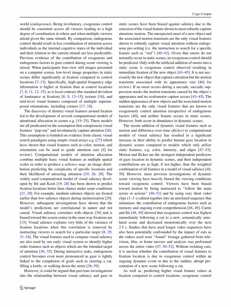
with an example shown in Fig. 1.

Edges

Considering the neurobiological evidence of early-vision

supporting lines, edge, contour, and center-surround oper-

ators [19, 26], the Sobel edge detector is an ideal binary

operator for detecting edges in images. It has also been

previously investigated as the primary feature employed in

a simple measure of saliency [78] and as part of

biologically inspired saliency maps [79, 80]. Sobel edge

detection performs a 2-dimensional spatial gradient mea-

surement on a luminance image using a pair of 3 9 3 pixel

convolution masks and an approximation to the gradient

defined by:

Gx ¼�1 0 þ1

�2 0 þ2

�1 0 þ1

264

375; Gy ¼

þ1 þ2 þ1

0 0 0

�1 �2 �1

264

375;

Gj j ¼ Gxj j þ Gy

�� �� ðSobel Edge DetectionÞ

ð1Þ

where Gx is the horizontal operator, Gy is the vertical

operator, and |G| is the approximation used as the edge map

[81]. A threshold parameter also controls which edges are

selected in the output edge map, throwing away all edges

above the threshold.

Corners

Complex features such as line-ends or corners where angles

in lines or sharp contours occur have been shown to be part

of early human visual processing [82] as well as shown to

be more salient than regions with purely straight edge or

simple feature stimuli [18]. Harris corners are well moti-

vated as corner detectors in the computer vision commu-

nity as they are invariant to rotation, scale, illumination,

and image noise [83]. Noble [84] also explains how the

Harris corner detector estimates image curvature and can

characterize two-dimensional surface features such as

junctions.

The Harris corner detector modifies the Moravec interest

operator [85] by using a first order derivative approxima-

tion to the second derivative. The algorithm uses autocor-

relation of image patches around an image pixel to find a

matrix A, denoted as the Harris matrix:

A ¼X

u

Xv

wðu; vÞ I2x IxIy

IxIy I2y

� �ðHarris Corner DetectionÞ

ð2Þ

where Ix and Iy are image gradients. Eigen values of this

matrix correspond to a low-contrast pixel (both Eigen

values are low), edge pixel (only one Eigen value is high),

or corner pixel (both Eigen values are high) label for the

given pixel depending upon their relationship [86]. We

considered only the case depicting corners. An example

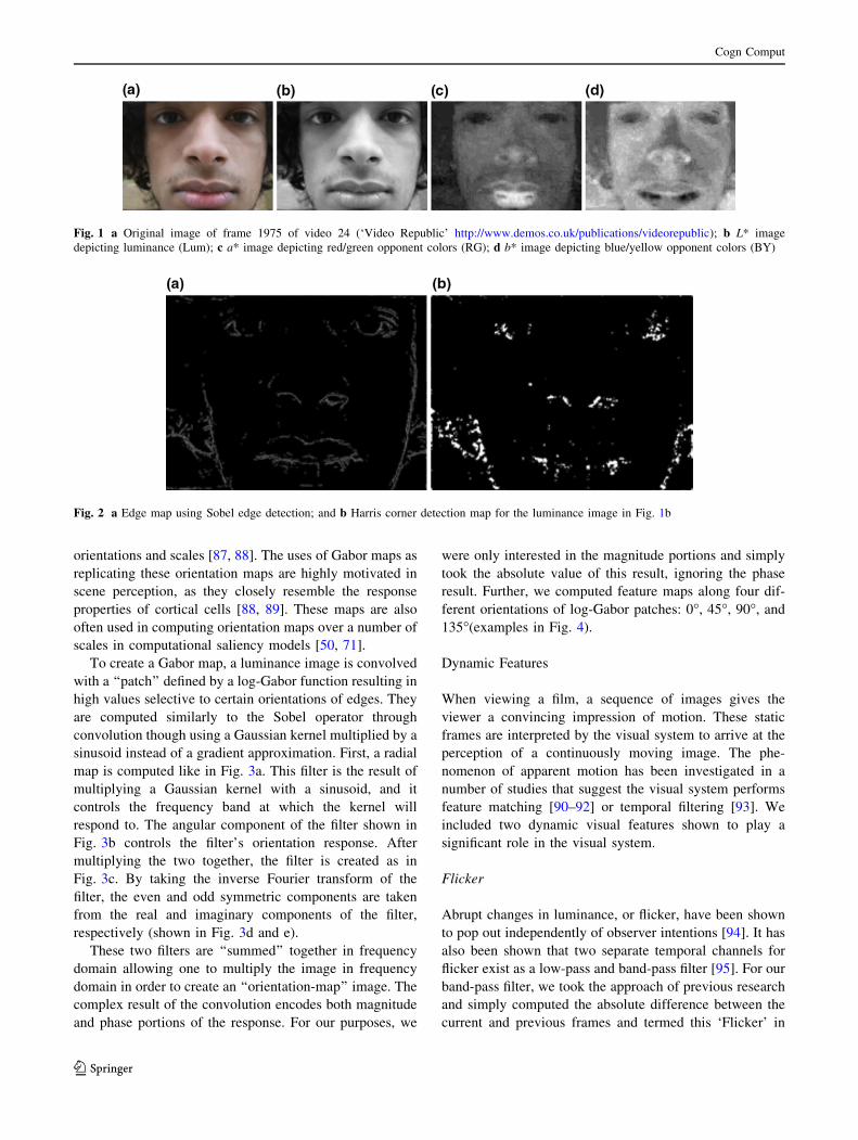
can be seen in Fig. 2.

Orientation Maps

Neurons in the primary visual cortex have been shown to

be selective to grating patterns tuned to different1 ICC.1: 2001-4, www.color.org.

Cogn Comput

123

orientations and scales [87, 88]. The uses of Gabor maps as

replicating these orientation maps are highly motivated in

scene perception, as they closely resemble the response

properties of cortical cells [88, 89]. These maps are also

often used in computing orientation maps over a number of

scales in computational saliency models [50, 71].

To create a Gabor map, a luminance image is convolved

with a ‘‘patch’’ defined by a log-Gabor function resulting in

high values selective to certain orientations of edges. They

are computed similarly to the Sobel operator through

convolution though using a Gaussian kernel multiplied by a

sinusoid instead of a gradient approximation. First, a radial

map is computed like in Fig. 3a. This filter is the result of

multiplying a Gaussian kernel with a sinusoid, and it

controls the frequency band at which the kernel will

respond to. The angular component of the filter shown in

Fig. 3b controls the filter’s orientation response. After

multiplying the two together, the filter is created as in

Fig. 3c. By taking the inverse Fourier transform of the

filter, the even and odd symmetric components are taken

from the real and imaginary components of the filter,

respectively (shown in Fig. 3d and e).

These two filters are ‘‘summed’’ together in frequency

domain allowing one to multiply the image in frequency

domain in order to create an ‘‘orientation-map’’ image. The

complex result of the convolution encodes both magnitude

and phase portions of the response. For our purposes, we

were only interested in the magnitude portions and simply

took the absolute value of this result, ignoring the phase

result. Further, we computed feature maps along four dif-

ferent orientations of log-Gabor patches: 0�, 45�, 90�, and

135�(examples in Fig. 4).

Dynamic Features

When viewing a film, a sequence of images gives the

viewer a convincing impression of motion. These static

frames are interpreted by the visual system to arrive at the

perception of a continuously moving image. The phe-

nomenon of apparent motion has been investigated in a

number of studies that suggest the visual system performs

feature matching [90–92] or temporal filtering [93]. We

included two dynamic visual features shown to play a

significant role in the visual system.

Flicker

Abrupt changes in luminance, or flicker, have been shown

to pop out independently of observer intentions [94]. It has

also been shown that two separate temporal channels for

flicker exist as a low-pass and band-pass filter [95]. For our

band-pass filter, we took the approach of previous research

and simply computed the absolute difference between the

current and previous frames and termed this ‘Flicker’ in

Fig. 1 a Original image of frame 1975 of video 24 (‘Video Republic’ http://www.demos.co.uk/publications/videorepublic); b L* image

depicting luminance (Lum); c a* image depicting red/green opponent colors (RG); d b* image depicting blue/yellow opponent colors (BY)

Fig. 2 a Edge map using Sobel edge detection; and b Harris corner detection map for the luminance image in Fig. 1b

Cogn Comput

123

our results section [19, 48]. As a low-pass filter, we used

the maximum of the previous 5 absolute frame differences

in order to capture slower frequency flickers (e.g. long-

term change) and termed this ‘Flicker-n’.

Object Motion

Cortical analysis of motion shows that the majority of V1

cells have selective response to motion in different orien-

tations before sending their output to the medial temporal

cortex [68]. It thus does not seem surprising to find that

evidence based on search efficiency has shown that our

visual system is able to notice moving objects even if we

are not looking for them. Phenomena associated with parts

of a scene that attract our attention are often given the label

‘‘pop out’’. Rosenholtz [75] has investigated these phe-

nomena in the context of motion by creating a measure of

saliency based on the extent to which the motion of a scene

differed from the general pattern of the scene. She showed

that a simple model measuring motion outliers can detect

motion pop out phenomena reliably. As well, Itti and Baldi

[77] have incorporated measures of motion into the most

recent versions of the iLab Neuromorphic Vision C??

Toolkit for their saliency computations. We investigated

this feature dimension by employing a classic computa-

tional vision algorithm for finding the motion of every

pixel in a scene.

Horn and Schunck [96] optical flow is a differential

method for calculating motion vectors in a brightness

image. The flow of an image, I, is defined by:

f ¼Z

Ix

Iy

� �VxVy

� �þ It

� �2

þ a rVxj j2þ rVy

�� ��2 !dxdy

ðOptical FlowÞð3Þ

where Ix, Iy, and It are the image derivatives, and Vx, and Vy

are the components of optical flow in the x (U in vector

notation) and y (V in vector notation) direction, respec-

tively. This method is often referred to as a global method

for calculating the optical flow, as the energy constraint

(the first term in Eq. 3) assumes gray value constancy and

does not depend on local image patches e.g. [97]. The

energy equation includes a second term known as the

‘‘smoothing’’ term in order to smooth flow where distor-

tions in the flow occur. This leads to better performance at

filling in ‘‘gaps’’ left from moving objects with similarly

textured regions than local methods.

In calculating our feature map, we discarded the vector

component of flow in opposing directions and only con-

sidered their magnitudes as we were interested in response

of motion and not their orientations. For example, -5 and

?5 horizontal flow (denoted U-flow) corresponds to flow in

the left and in the right direction, respectively. We disre-

garded this distinction and considered both as U-flow with

Fig. 3 The process for creating a log-Gabor kernel for 0� (left to

right): a the radial map computed from multiplying a sinusoid with a

Gaussian kernel; b the orientation of the kernel set for 0�; c the result

of multiplying the radial (a) and orientation (b) maps; d the even

symmetric component of the log-Gabor filter taken from the real part

of the inverse fourier transform of the kernel; e the corresponding odd

symmetric component taken from the imaginary component of the

kernel

Fig. 4 Gabor-oriented maps for a 0�, b 45�, c 90�, and d 135� for the luminance image in Fig. 1b

Cogn Comput

123

magnitude 5 (and similarly, with vertical or V-Flow).

Examples are shown in Fig. 5.

Results

Visual Features at Baseline Foveations Versus Actual

Foveations

To account for intrinsic variations in each film as well as

central bias, we created a baseline measure by sampling

with replacement from the distribution of all subject bin-

ocular foveations for each video similar to Henderson et al.

[8] (see Fig. 6 for distributions). Thus, for each frame,

baseline foveations were sampled with replacement from

the distribution of all foveations across the duration of the

movie. The number of baseline foveations sampled for

each frame matched the number of valid actual foveations

for that frame. Examples of actual subject and baseline

foveations are shown in Fig. 7.

Selection of Visual Features During Dynamic Scene

Viewing

In order to assess the selection of visual features, we fol-

lowed the approach of previous research [15, 47, 52] by

employing a signal detection framework based on the

Receiver Operator Characteristic (ROC) curve [99]. This

metric has a number of benefits when investigating fixated

feature values: (1) capability of accounting for the vari-

ability of actual and baseline foveations, (2) independence

from the number of data points used, (3) ability to recover

the non-linear statistics of different visual features [98] via

a dense sampling (i.e. more samples of signal/noise ratio),

(4) accounts for the bias of photographers to place salient

objects closer to the center of the composition [15], and

(5) accounts for the distribution of foveations toward the

center of an image by comparing actual foveations against

a sampled baseline (see Fig. 6 for example foveation dis-

tributions, and Fig. 7 for example baseline foveations).

We employed the ROC in order to specify how well

actual foveations (signal) could be separated from baseline

foveations (noise) on each feature dimension. Each feature

map was systematically thresholded from its minimum to

maximum value. At each threshold, actual and baseline

locations were identified as either having mean values

above (‘‘1’’) or below the threshold (‘‘0’’). The correct

labeling of an actual location as ‘‘1’’ signified a ‘‘hit’’

whereas ‘‘0’’ was a ‘‘miss’’. If a threshold also labeled a

baseline location as ‘‘1’’ it constituted a ‘‘false alarm’’. If

the systematic thresholding produced as many hits as false

alarms, then the feature dimension could not be said to

distinguish between the signal (actual locations) and the

noise (baseline locations) and, therefore, could not predict

foveation.

As many of the feature spaces contained heavily skewed

distributions and no assumptions were made concerning the

feature space distributions, we used 200 non-linearly

spaced thresholds in order to recover the tail ends of the

feature distribution and model a tighter fit to the underlying

ROC curve. Plotting a false alarm rate (baseline foveations

as a ‘‘1’’) versus an actual hit rate (actual subject foveations

as ‘‘1’’) provided a ROC curve describing the nature of the

signal noise ratio across all thresholds. A feature dimension

that performed at chance at separating signal from noise

would thus create a straight line with hit rate being iden-

tical to the false alarm rate, i.e. a gradient of 1. By com-

parison, if a feature increased in its ability to discriminate

actual from sampled foveation locations, the line would

curve toward (0, 1). The greater the curve, the greater the

area under the curve (AUC), and the greater the ability of a

feature to discriminate between hits and false alarms. Thus,

the curve can be accurately summarized by its AUC where

0.5 corresponds to chance (a linear line), and 1.0 corre-

sponds to a perfect discrimination.

We classified attended visual features by investigating

the AUC of a ROC analysis. Table 1 shows the results

computed based on Fig. 8. A number of interesting findings

were present. Luminance, Red/Green, and Blue/Yellow

were just above chance although their respective standard

deviations were much higher suggesting both luminance

Fig. 5 a High-pass flicker (Flicker); b low-pass flicker (Flicker-N); c horizontal optical flow (U-Flow); d vertical optical flow (V-Flow) for the

frame in Fig. 1a

Cogn Comput

123

and opponent color contrast as important selected features.

Edges performed at chance though this was likely because

of the very sparse response of the edge-maps at the selected

kernel size of 3 9 3 and selectivity threshold of the Sobel

implementation.

We found little differences between orientations and

their standard deviations though both feature sets were

selected more than Luminance, Red/Green, and Blue/

Yellow. High-pass Flicker performed just below the

Gabors though the low-pass measure of Flicker, Flicker-N,

Fig. 6 a Binocular foveation

distributions for each movie

represented as heat maps

(normalized 0–1, blue-red).

b Example scenes for each

movie with clustering of gaze

and individual gaze locations

overlaid; c histograms of

weighted cluster covariances for

each film. (see Appendix 2 for

the remaining films used)

Cogn Comput

123

as well as its standard deviations performed on par with

Luminance Std Dev, Red/Green Std Dev, Blue/Yellow Std

Dev, Harris Corners and Harris Corners Std Dev, sug-

gesting a higher selection toward motions occurring over a

longer interval. Optical flow features (U/V flow and their

standard deviations) performed the highest (0.67, 0.68,

0.67, 0.67) of our investigated features. This is strong

evidence for motion as the most predictive visual feature of

foveations during dynamic scene viewing.

Within Subject Categorical Analysis Between Tight

and Loosely Clustered Gaze

The phenomena of attention capture have been studied in

the context of natural scene viewing suggesting that abrupt

Fig. 7 Example actual (cross) and baseline (circle) subject foveations for videos 1, 2, 15, and 24 (clockwise from top left)

Table 1 The area under the receiver operator characteristic curve

(AUC) for feature values 4� around gaze locations

Feature AUC

Luminance 0.526377

Luminance Std Dev 0.630167

Red/Green 0.546701

Red/Green Std Dev 0.606843

Blue/Yellow 0.531026

Blue/Yellow Std Dev 0.608749

Sobel edges 0.530066

Sobel edges Std Dev 0.530062

Gabor at 0� 0.604528

Gabor at 0� Std Dev 0.608238

Gabor at 45� 0.608014

Gabor at 45� Std Dev 0.61033

Gabor at 90� 0.596378

Gabor at 90� Std Dev 0.599987

Gabor at 135� 0.607202

Gabor at 135� Std Dev 0.609411

Harris corners 0.636152

Harris corners Std Dev 0.646601

Flicker 0.584435

Flicker Std Dev 0.589377

Flicker (N-prev) 0.619877

Flicker (N-prev) Std Dev 0.645487

U optical flow 0.670323

U optical flow Std Dev 0.675288

V optical flow 0.66854

V optical flow Std Dev 0.673837

Fig. 8 ROC curves for a selection of the features @ 4�. Higher

curves toward point (0, 1) are better. Chance is 0.5. Best viewed in the

online version of the publication in color. Refer to Table 1 for all

feature results

Cogn Comput

123

onsets of distinct objects, unique colors or shapes, or cer-

tain patterns of motions are particularly selective of

attention [43]. During these involuntary moments of

attention capture, viewers are thus expected to cluster in

similar locations of a natural scene. We investigated a

measure of clustering of eye movements in order to infer

whether feature values are more predictive of subject eye

movements during moments of tight clustering.

Only a few known studies have looked into clustering

eye movements. Privitera and Stark [100] compared

actual and simulated foveations using k-means clustering.

Latimer [101] used a form of k-means based on histograms

of foveation durations in an effort to classify partitions

more robustly, although he comments that k-means clus-

tering often produces inconsistent results. Santella and

DeCarlo [102] quantified visual interest via a mean-shift

clustering framework. Though this method is robust to

noise and does not require the number of clusters a priori, it

does require additional tuning of parameters based on

temporal and spatial scales.

Reported success of density estimation via expectation/

maximization [103] of a parametric family distribution in

Sawahata et al. [59] prompted us to use mixture models as

our clustering method. Sawahata et al. investigated an

entropy measure calculated from the log likelihood of a

mixture model in order to determine viewer comprehension

during dynamic scene viewing. This method when com-

bined with model selection and enough data points can

produce consistent results that are robust to noise and does

not require the number of clusters a priori (which is the

main drawback of k-means clustering). A prior model of the

distribution of data is required in order to accurately tune

the parameters during expectation/maximization. We used

Gaussians as our parametric prior since they have been

shown to account for much of the variance in the center bias

apparent in viewing strategy and photographer bias during

dynamic image viewing [66]. The resulting model is more

commonly known as a Gaussian Mixture Model (GMM).

GMMs represent a collection of unlabeled data points as

a mixture of Gaussians each with a separate mean,

covariance, and weight parameter. For our purposes, we

used this model to classify moments of tight and loose

clusters of eye movements across subjects by calculating

the sum of the weighted cluster covariances (i.e. the sum

over all cluster covariances weighted by the cluster

weight). Note that by using model selection, the problem of

over-fitting a model to noise, i.e. zero covariance Gaussians

centered at fixations, is dealt with in the BIC term which

penalizes the number of clusters. We refer the reader to

Bishop [103] and Sawahata et al. [59] for more details on

GMM modeling and model selection. A few example stills

are shown in Fig. 9 depicting the GMMs extracted from

this algorithm.

We investigated the correlation between frames eliciting

tightly clustered data with the low-level features that

encode them. We first classified all frames by their

weighted cluster covariance. Then, we categorized ‘‘tightly

clustered’’ (low covariance) and ‘‘loosely clustered’’ (high

covariance) frames in order to see whether actual subject

eye movements were more or less predictive of low-level

features. If visual features are correlated with where we

attend, then moments when everybody looks in the same

place should also correlate with a peak in the feature space.

As well, we should expect to find less influence of visual

features during moments when there is less synchrony

between viewers (i.e. high covariance). To test this

hypothesis, we used Gaussian Mixture Models (GMMs)

Fig. 9 Example stills from clustering binocular eye tracking data on

video 16. Blue values correspond to 0.0 and red to 1.0. The first

example still uses the values of the GMM as an alpha-map layer

providing a ‘peek-through’ effect. Notice the robustness to noise

given the large number of data samples in the first still (original movie

image of Ice Age 3 Trailer Copyright Twentieth Century Fox)

Cogn Comput

123

using a Bayesian Information Criterion (BIC) model

selection on the frame-by-frame eye movements across all

subjects.

To define a moment of synchrony, we investigated the

distribution of the weighted Gaussian covariance. This

measure has the benefit of measuring the distribution of eye

movements in a given frame (in terms of the covariance) as

well as indicating the strength of each cluster to model eye

movements (in terms of the weight parameter). The his-

togram of the weighted covariances for each film (depicted

in Fig. 6 and Appendix 2) clearly indicates a large degree

of variation in the degree of clustering. Some films, such as

film 15 exhibit tight clustering throughout their entire

viewing time, whereas other films, such as film 26 exhibit

very little clustering.

To classify tightly and loosely clustered frames, we used

the median of the distribution of all frames for all movies’

weighted covariance value, which is centered at 230 (mean

360, sigma 330; see Fig. 10). Taking only the frames

greater than and less than the median, we were able to

consider whether any features could be distinguished when

compared to a random baseline measure in a categorical

analysis of tightly and loosely clustered frames.

Splitting gaze according to the degree of clustering

revealed a systematic increase in the ability of all visual

features to discriminate actual from baseline foveations for

tight clusters. AUC values were higher for tight clusters

than loose clusters in all features. For example, vertical

optical flow AUC values increased from 0.63 in loose

clusters to 0.71 in tight ones, indicating that during these

moments 71% of actual gaze locations could be discrimi-

nated from baseline locations by this feature alone. This

suggests that the selection of visual features is more pre-

dominant as eye movements across multiple subjects are

clustered tightly together than during loosely clustered

scenes. As in the comparison with baseline subjects across

all frames, we found the most significant AUC values for

motion. As well, the standard deviation of each feature had

a higher response than the feature strength alone (Table 2).

Selection of Visual Features as a Function of Clustering

The median split of cluster covariance indicated that tighter

clusters correspond with higher AUC values. To examine

this relationship further, the distribution of cluster covari-

ances was further subdivided into seven bins of width 75

and a maximum of 525 (careful examination of the range of

weighted cluster covariances across movies indicated very

few moments above 525; Appendix 2).

Fig. 10 A plot depicting a histogram distribution of all frames

weighted covariance measure. To classify tight and loosely clustered

frames, we used the median of the distribution of all frames for all

movies weighted covariance value, which is centered at 230 (mean

360, sigma 330)

Table 2 The area under the curve (AUC) for each feature dimension

split according to weighted cluster covariance

Feature Loose clusters

(AUC)

Tight clusters

(AUC)

Luminance 0.505682 0.545678

Luminance Std Dev 0.597268 0.66307

Red/Green 0.515643 0.576606

Red/Green Std Dev 0.578396 0.633503

Blue/Yellow 0.519821 0.542573

Blue/Yellow Std Dev 0.582418 0.634017

Sobel edges 0.520351 0.53968

Sobel edges Std Dev 0.520349 0.539674

Gabor at 0� 0.57853 0.630239

Gabor at 0� Std Dev 0.581526 0.634526

Gabor at 45� 0.579087 0.636106

Gabor at 45� Std Dev 0.580594 0.639148

Gabor at 90� 0.568905 0.622719

Gabor at 90� Std Dev 0.571076 0.627879

Gabor at 135� 0.578521 0.635135

Gabor at 135� Std Dev 0.580133 0.638033

Harris corners 0.602542 0.669791

Harris corners Std Dev 0.612087 0.680933

Flicker 0.560667 0.60797

Flicker Std Dev 0.564554 0.614068

Flicker (N-prev) 0.589983 0.650598

Flicker (N-prev) Std Dev 0.61298 0.678218

U optical flow 0.636065 0.705184

U optical flow Std Dev 0.640588 0.710575

V optical flow 0.630426 0.706752

V optical flow Std Dev 0.635424 0.712136

Loose clusters and tight clusters are defined as [ are \ the median

weighted cluster covariance (230), respectively

Cogn Comput

123

The AUC results are presented graphically as a function

of each bin in Fig. 11. The figure clearly demonstrates an

inverse curvilinear relationship between weighted cluster

covariance and AUC. Each feature presents a clear trend

toward higher AUC values for smaller bin sizes, suggesting

that as clusters are tighter, the selection of visual features

are more predominant. Notably, the order of the most pre-

dominantly selected visual features stays similar in each bin

size with motion topping the list in each bin. For example,

during moments of tightest clustering (0–75), the percent-

age of actual locations correctly discriminated from base-

line locations by vertical flow increases from *64 to 77%.

The influence of Cinematic Cuts on the Selection

of Visual Features

Previous research has suggested that a strong central bias

exists based on photographer bias and viewing strategy [65,

66] producing high inter-observer consistency, i.e. a metric

determining the ‘‘spread’’ in eye movements, immediately

following a cinematic cut. Further, Carmi and Itti’s [48]

research suggests that the selection of saliency and motion

contrasts is highest during high inter-observer consistency

following semantically unrelated MTV-style jump cuts.

However, our content did not control for top–down behavior

and thus would include influences from prior scene knowl-

edge and continuity editing. That is, scene content may or

may not be related on either side of a cinematic cut.

Given previous research findings, a possible explanation

for the higher selection of visual features during tightly

clustered scenes is that these clusters may be most pre-

dominant following a cinematic cut where during seman-

tically unrelated content, visual feature selection has been

shown to be the highest. As such, our results in the pre-

vious section could either have been indicative of

(1) photographer bias and viewing strategy, where tightly

clustered eye movements following cinematic cuts explain

higher selection of visual features during dynamic scene

viewing; (2) spontaneous clustering of eye movements dur-

ing ongoing dynamic scene viewing; or (3) both 1 and 2.

In order to investigate this issue further, we took the

same approach as Carmi and Itti [48] in investigating the

first saccades following an abrupt cinematic cut. We hand-

coded every cinematic cut for each of our 26 movies

excluding those with cuts that are not distinguished by

abrupt changes to a single composition (e.g. multiple

composite videos or alpha/chromaticity blending). Plotting

the weighted cluster covariance as a function of time fol-

lowing a cinematic cut revealed a tendency for viewers to

cluster tightly together with a mean weighted covariance

value approaching 250 during the first 533 ms (Fig. 12).

Further, plotting the Euclidean distance of foveations to the

center of the display revealed a central bias 333 ms fol-

lowing a cut (Fig. 13).

To investigate whether the peak in feature selection was

caused by the tight clustering immediately following a cut,

we analyzed three time periods such that the center of these

bins were closely centered to the observed clustering and

central bias at 333 and 533 ms: 0–200 ms, 200–400 ms,

and 400–600 ms following a cut. The results show that,

contrary to the hypothesis that clustering following cuts is

the primary explanation for higher selection of visual fea-

tures during dynamic scene viewing, there is no noticeable

peak close to the previous AUC value in feature selection

for any degree of clustering immediately following the cut

(0–200 ms) or in either of the other two time windows

Fig. 11 Area under ROC

curves (AUC) as a function of

weighted cluster covariance

(bins = 75)

Cogn Comput

123

(Fig. 14). The ranking of selection for feature dimensions

remains the same, with motion features contributing most

to gaze location, but the effect of greater feature selection

during tighter clustering behavior is greatly weakened if

not entirely gone. This suggests that the tight clustering

observed immediately following cuts in our film corpus is

caused by a central tendency (Fig. 13) and not exogenous

control by visual features. Given the absence of a strong

relationship between clustering and feature selection

immediately following cuts, the relationship observed

throughout films (Fig. 11) cannot be fully attributed to cuts

and appears to mostly occur spontaneously during ongoing

dynamic scenes.

Fig. 12 Weighted cluster covariance as a function of time since a cut.

Error bars represent ±1 SE

Fig. 13 Euclidean distance between foveations and screen center as a

function of time since a cut

Fig. 14 AUC presented as a function of weighted cluster covariance

at time points a 0–200 ms, b 200–400 ms, and c 400–600 ms

following a cut

Cogn Comput

123

Discussion

The present study investigated the contribution of visual

features to gaze location during free-viewing of dynamic

scenes using a signal detection framework. The results

indicated that foveated locations could be discriminated

from control locations by mid-level visual features with

motion contrasts as the strongest predictors, confirming

previous evidence that motion is the strongest independent

predictor of gaze location in dynamic scenes [48, 50]. The

next strongest predictors following motion were corners

suggesting a strong role in mid-level visual features to

predict gaze location. High-pass flicker performed just

below Gabor orientations although the low-pass measure of

flicker, flicker-n, as well as their standard deviations per-

formed on par with the standard deviations of luminance,

color, and corners, suggesting a stronger selection for

changes occurring over a longer interval than shorter ones.

Low-level visual features such as luminance and color were

not able to discriminate foveated from non-foveated loca-

tions as their AUC value was around chance, 0.5. However,

as their respective contrasts (i.e. standard deviations) were

much higher, this would suggest that both luminance and

opponent color contrast are important selected features.

Edges performed at chance although a number of issues

were present. First, the kernel size of 3 9 3 may not have

been ideal to produce a range of edge values. Second, the

process of thresholding edge values from the Sobel operator

may also not have been ideal and instead a non-maximum

suppression and hysteresis procedure would produce edges

closer to perceptual boundaries. Torre and Poggio [104] also

note that filtering of a sampled image prior to differentiation

is necessary to regularize the problem of computing deriva-

tives in an intensity image. This could be achieved by a band-

pass (e.g. sinc or prolate) or minimal uncertainty (e.g. Gabor

or Hermite function) filter. However, each filter is noted to

have different merits and trade-offs. Further, a number of

other edge operators are predominant in the computer vision

community based on gradients, phase congruency, or second

derivatives, again each with their own merits and trade-offs.

These issues could be investigated in more depth in future

studies to reproduce the selection of edges by gaze as shown

in previous static studies [7, 8, 15, 105, 106].

Gaze Clustering

The selection of all visual features increased as the degree

of clustering of gaze increased. During these moments, the

ordering of feature selectivity remained the same, but their

degree of contribution increased considerably. For exam-

ple, motion increased from an overall average AUC of

*0.64 to 0.77 during moments of tightest clustering. This

indicates that during these moments 77% of foveated

locations could be distinguished from control locations via

motion information alone. On the face of it, this relation-

ship between clustering and feature contributions to gaze

would seem to suggest bottom–up gaze control: universal

involuntary capture of gaze by a point of high motion. Such

a causal interpretation was proposed by Carmi and Itti [48]

for moments during dynamic scene viewing when all top–

down influence was removed, e.g. immediately following a

cut to a semantically unrelated dynamic scene. However,

identifying similar moments in our stimuli revealed no

relationship between visual features and gaze clustering

during the first second following a cut. Instead, clustering

following cuts seems to be caused by a tendency to saccade

to the screen center. A similar central bias has previously

been reported during dynamic scene viewing [52] and is

thought to be due to compositional bias, e.g. framing focal

objects at screen center, and a viewing strategy of using the

screen center to reorient to new scenes [66]. Carmi and Itti

[48] did not control for central bias in their analysis as their

control locations were sampled uniformly across the

screen. Subsequent analysis of similar videos in their lab

showed that there was a strong central tendency immedi-

ately following a cut and they suggested that future studies

should sample control locations from this centrally biased

baseline in order to identify the independent contributions

of visual features [66]. The ROC analysis performed in the

present study uses such a centrally-based baseline by

sampling from each participants own gaze locations at

another time point in time during the same video. With the

contribution of screen center subtracted from the analysis,

we found no contribution of visual features to gaze clus-

tering immediately following cuts.

Bottom–Up Versus Top–Down Control During

Ongoing Dynamic Scenes

The moments of clustering observed in our study occurred

spontaneously during ongoing dynamic scenes. We have

previously observed this phenomenon and referred to it as

Attentional Synchrony [60]. The increase in visual feature

contributions during Attentional Synchrony may suggest

that gaze is involuntarily captured by sudden unexpected

visual features such as object appearances or motion onsets

[43–46]. Bottom–up control of gaze by unexpected events

in the real-world such as the sudden approach of a predator,

car, or projectile has clear evolutionary advantages. How-

ever, it is difficult to separate the bottom–up influence of

such visual events from top–down prioritization due to their

Cognitive Relevance [8, 34, 107]. As visual features such as

luminance, contrast, and edge density in scenes have been

shown to correlate with the rated semantic informativeness

of a location [8], gaze may be guided toward an object due

to its cognitive relevance, and the corresponding peak in

Cogn Comput

123

feature values around foveation may simply be a by-product

of this correlation. For example, a recent study by Vincent

et al. [108] used mixture modeling to isolate the indepen-

dent contributions of low and high-level visual features to

fixations in static scenes. The authors found that low-level

features in isolation contributed very little to fixation

location compared to the much larger contribution of cen-

tral bias and preference for foreground objects.

A quick survey of the visualized clusters observed in our

study suggests that clusters often coincide with semanti-

cally rich objects such as eyes, faces, hands, vehicles, and

text (see Figs 6, 7, 10 and Appendix 1 for examples). Gaze

also appears to be allocated over time in response to visual

events such as human bodily movements, gestures, con-

versations, and interactions with other humans and objects.

Further, perception of complex visual events is known to

operate in a predictive manner based on previous exposure

to similar events [109] but is also predicted by disconti-

nuities of motion [110, 111].

When visual events are recorded for presentation in

Television or Film, scenes may be composed to focus

attention toward the event by manipulating visual features

such as lighting, color, focal depth, central framing, and

motion of the object relative to the background and frame

[112]. Such composed dynamic scenes were used in this and

previous studies [48, 49, 51, 52, 66]. As such, the compo-

sitional manipulations of the image may increase the cor-

relation between gaze and visual features though would not

necessarily imply causation. A particular location may be

foveated because it is cognitively relevant to the viewer and

not because of a high contrast in visual features. The cog-

nitive relevance of an object may remain even in the absence

of distinct visual features. Static [113, 114] and dynamic

scene studies [115] in which semantically rich regions have

been filtered to remove visual features have shown that

participants continue to attend to the semantically rich

regions even though these regions are heavily obscured,

further suggesting that top–down factors such as object

semantics are the main contributors to gaze allocation.

Predicting Gaze Location in Dynamic Scenes

Is it possible to predict gaze location in dynamic scenes? An

ideal model of gaze location in dynamic scenes would

robustly locate the causal root of gaze allocation in terms of

cognitively relevant scene semantics. This would entail

robustly computing object and scene semantics relevant to a

viewer’s task and expertise given prior memory and encod-

ing of the scene. However, the natural correlation between

scene semantics and motion in natural scenes may provide a

reasonably reliable method for predicting gaze location. In a

natural dynamic scene viewed from a static vantage point

(e.g. camera position), the only focused motion in the scene

will be produced by animate objects such as people, animals,

and vehicles. Identification of the motion created by these

objects may provide a simple method of automatically

parsing the objects from the background and identifying

candidate gaze locations. The predictions of such a model

will remain valid as long as (a) objects in the scene continue

moving; (b) the background and camera remain stationary;

and (c) top–down and bottom–up factors remain correlated

such as during free-viewing. It is currently not known what

effect the de-correlation of top–down and bottom–up factors

would have on gaze allocation. If participants were instruc-

ted to search for an inanimate object, would this top–down

instruction be able to completely override the bottom–up

contribution of features such as motion? Only by pitting top–

down and bottom–up factors against each other during

dynamic scene viewing would we be able to understand their

relative contributions and evaluate how reliable a model

based solely on bottom–up features would be in predicting

gaze location.

Acknowledgments The authors would like to thank members of the

Edinburgh Visual Cognition laboratory including Antje Nuthmann

and George Malcolm for their comments and feedback, and Josie

Landback for running experiments. This project was funded by the

Leverhulme Trust (Ref F/00-158/BZ) and the ESRC (RES-062-23-

1092) awarded to John M. Henderson.

Appendix 1

See Table 3.

Table 3 List of videos used in this study

Number Video type Width Height Duration

(s)

Cuts ASL

(s)

1 Advertisement 1,024 768 41 0 41

2 Advertisement 1,024 768 40 0 40

3 Advertisement 1,280 720 72 43 1.6

4 Advertisement 848 480 30 7 4.2

5 Documentary 1,280 720 109 13 8.4

6 Documentary 1,280 720 98 58 1.7

7 Documentary 1,280 720 152 11 13.1

8 Documentary 1,280 720 106 27 7.8

9 Documentary 1,280 720 86 14 6.1

10 Documentary 1,280 704 169 23 7.3

11 Game trailer 1,280 720 124 N/A N/A

12 Game trailer 1,280 720 103 62 1.6

13 Game trailer 1,280 720 110 76 1.4

14 Game trailer 1,280 548 203 30 6

15 Home movie 960 720 55 0 55

16 Movie trailer 1,280 690 109 18 6

17 Movie trailer 1,280 688 99 94 1

Cogn Comput

123

Appendix 2

Continuation of Fig. 6.

Table 3 continued

Number Video type Width Height Duration

(s)

Cuts ASL

(s)

18 Music video 704 576 27 N/A N/A

19 Music video 1,024 576 216 N/A N/A

20 Music video 1,280 720 43 N/A N/A

21 News 768 576 102 23 4.4

22 News 768 576 66 16 4.1

23 News 1,080 600 85 N/A N/A

24 News 960 720 209 N/A N/A

25 News 768 576 217 31 5.3

26 Time-lapse 1,280 720 47 N/A N/A

Columns left to right: Video number; Video Type; Width (pixels);

Height (pixels); Duration (s); Number of cuts (n.b. N/A unable to

calculate due to use of digital effects); Average Shot Length (ASL; s).

Our study used 26 different films ranging a total of 549 edits used in

the analysis of cinematic features, at 30 fps and 333 ms bins over 1 s

(i.e. 5,490 frames of data per bin)

Cogn Comput

123

References

1. Findlay JM. Eye scanning and visual search. In: Henderson JM,

Ferreira F, editors. The interface of language, vision, and action:

eye movements and the visual world. New York, NY, US:

Psychology Press; 2004. p. 134–59.

2. Findlay JM, Gilchrist ID. Active vision: the psychology of

looking and seeing. Oxford: University Press; 2003.

3. Henderson JM. Regarding scenes. Curr Dir Psychol Sci.

2007;16(4):219–22.

4. Wolfe JM, Horowitz TS. What attributes guide the deployment

of visual attention and how do they do it? Nat Rev Neurosci.

2004;5:1–7.

5. Buswell GT. How people look at pictures: a study of the psy-

chology of perception in art. Chicago: University of Chicago

Press; 1935.

6. Yarbus AL. Eye movements and vision. New York: Plenum

Press; 1367.

7. Baddeley RJ, Tatler BW. High frequency edges (but not con-

trast) predict where we fixate: a Bayesian system identification

analysis. Vision Res. 2006;46:2824–33.

8. Henderson JM, et al. Visual saliency does not account for eye

movements during visual search in real-world scenes. In: van

Gompel RPG, et al., editors. Eye movements: a window on mind

and brain. Oxford: Elsevier; 2007. p. 537–62.

9. Krieger G, et al. Object and scene analysis by saccadic eye-

movements: an investigation with higher-order statistics. Spat

Vis. 2000;13(2–3):201–14.

10. Mannan S, Ruddock KH, Wooding DS. Automatic control of

saccadic eye movements made in visual inspection of briefly

presented 2-D images. Spat Vis. 1995;9(3):363–86.

11. Mannan SK, Ruddock KH, Wooding DS. The relationship

between the locations of spatial features and those of fixations

made during visual examination of briefly presented images.

Spat Vis. 1996;10(3):165–88.

12. Mannan SK, Ruddock KH, Wooding DS. Fixation sequences

made during visual examination of briefly presented 2D images.

Spat Vis. 1997;11(2):157–78.

13. Parkhurst DJ, Niebur E. Scene content selected by active vision.

Spat Vis. 2003;6:125–54.

14. Reinagel P, Zador AM. Natural scene statistics at the centre of

gaze. Netw Comput Neural Syst. 1999;10:1–10.

15. Tatler BW, Baddeley RJ, Gilchrist ID. Visual correlates of fix-

ation selection: effects of scale and time. Vision Res.

2005;45(5):643–59.

16. Parkhurst DJ, Niebur E. Texture contrast attracts overt visual

attention in natural scenes. Eur J Neurosci. 2004;19:783–9.

17. Barth E, Zetsche C, Rentschler I. Intrinsic two-dimensional

features as textons. J Opt Soc Am A Opt Image Sci Vis. 1998;

15:1723–32.

18. Zetzsche C, et al. Investigation of a sensorimotor system for

saccadic scene analysis: an integrated approach. In: Feifer RP,

editor. From animals to animats 5. Cambridge, MA: MIT Press;

1998. p. 120–6.

19. Itti L, Koch C. Computational modelling of visual attention. Nat

Rev Neurosci. 2001;2(3):194–203.

20. Navalpakkam V, Itti L. Modeling the influence of task on

attention. Vision Res. 2005;45(2):205–31.

21. Parkhurst D, Law K, Niebur E. Modeling the role of salience in the

allocation of overt visual attention. Vision Res. 2002;42(1):107–23.

22. Pomplun M, Reingold EM, Shen J. Area activation: a compu-

tational model of saccadic selectivity in visual search. Cogn Sci.

2003;27:299–312.

23. Rao RPN, et al. Eye movements in iconic visual search. Vision

Res. 2002;42(11):1447–63.

24. Sun Y, et al. A computer vision model for visual-object-based

attention and eye movements. Comput Vis Image Underst. 2008;

112(2):126–42.

25. Zelinsky GJ. A theory of eye movements during target acqui-

sition. Psychol Rev. 2008;115(4):787–835.

26. Koch C, Ullman S. Shifts in selective visual-attention: towards

the underlying neural circuitry. Hum Neurobiol. 1985;4(4):

219–27.

27. Treisman AM, Gelade G. Feature-integration theory of atten-

tion. Cogn Psychol. 1980;12(1):97–136.

28. Itti L. A saliency-based search mechanism for overt and covert

shifts of visual attention. Vision Res. 2000;40:1489–506.

29. Foulsham T, Underwood G How does the purpose of inspection

influence the potency of visual salience in scene perception?

2007.

30. Einhauser W, Spain M, Perona P. Objects predict fixations better

than early saliency. J Vis. 2008;8(14):11–26.

31. Chen X, Zelinsky GJ. Real-world visual search is dominated by

top-down guidance. Vision Res. 2006;46(24):4118–33.

32. Foulsham T, Underwood G. Can the purpose of inspection

influence the potency of visual salience in scene perception?

Perception. 2006;35:236.

33. Foulsham T, Underwood G. What can saliency models predict

about eye movements? Spatial and sequential aspects of fixa-

tions during encoding and recognition. J Vis. 2008;8(2).

34. Henderson JM, Malcolm GL, Schandl C. Searching in the dark:

cognitive relevance drives attention in real-world scenes. Psy-

chon Bull Rev. 2009;16:850–6.

35. Henderson JM, et al. Eye movements and picture processing

during recognition. Percept Psychophys. 2003;65(5):725–34.

36. Hayhoe M, Land M. Coordination of eye and hand movements

in a normal visual environment. Invest Ophthalmol Vis Sci.

1999;40(4):S380.

37. Land MF, Hayhoe M. In what ways do eye movements con-

tribute to everyday activities? Vision Res. 2001;41(25–26):

3559–65.

38. Land MF, Lee DN. Where we look when we steer. Nature.

1994;369(6483):742–4.

39. Land MF, McLeod P. From eye movements to actions: how

batsmen hit the ball. Nat Neurosci. 2000;3(12):1340–5.

40. Yantis S. Control of visual attention. In: Pashler H, editor.

Attention. London: Psychology Press; 1998. p. 223–56.

41. Yantis S, Hillstrom AP. Stimulus-driven attentional capture:

evidence from equiluminant visual objects. J Exp Psychol Hum

Percept Perform. 1994;20(1):95–107.

42. Yantis S, Jonides J. Abrupt visual onsets and selective attention:

evidence from visual search. J Exp Psychol Hum Percept Per-

form. 1984;10(5):601–21.

43. Brockmole JR, Henderson JM. Prioritization of new objects inreal-world scenes: evidence from eye movements. J Exp Psychol

Hum Percept Perform. 2005;31(5):857–68.

44. Brockmole JR, Henderson JM. Object appearance disappear-

ance, and attention prioritization in real-world scenes. Psychon

Bull Rev. 2005;12(6):1061–7.

45. Matsukura M, Brockmole JR, Henderson JM. Overt attentional

prioritization of new objects and feature changes during real-

world scene viewing. Vis Cogn. 2009;6(7):835–55.

46. Simons DJ. Attentional capture and inattentional blindness.

Trends Cogn Sci. 2000;4(4):147–55.

47. Berg DJ, et al. Free viewing of dynamic stimuli by humans and

monkeys. J Vis. 2009;9(5):1–15.

48. Carmi R, Itti L. Visual causes versus correlates of attentional

selection in dynamic scenes. Vision Res. 2006;46(26):4333–45.

49. Carmi R, Itti L. The role of memory in guiding attention during

natural vision. J Vis. 2006;6(9):898–914.

Cogn Comput

123

50. Itti L. Quantifying the contribution of low-level saliency to

human eye movements in dynamic scenes. Vis Cogn. 2005;

12(6):1093–123.

51. Itti L. Quantitative modelling of perceptual salience at human

eye position. Vis Cogn. 2006;14(4–8):959–84.

52. Le Meur O, Le Callet P, Barba D. Predicting visual fixations on

video based on low-level visual features. Vision Res.

2007;47(19):2483–98.

53. t’Hart BM, et al. Gaze allocation in natural stimuli: comparing

free exploration to head-fixed viewing conditions. Vis Cogn.

2009;17(6/7):1132–58.

54. Goldstein RB, Woods RL, Peli E. Where people look when

watching movies: do all viewers look at the same place? Comput

Biol Med. 2007;37(7):957–64.

55. Hasson U, et al. Neurocinematics: the Neuroscience of Film.

Proje J Movies Mind. 2008;2(1):1–26.

56. Marchant P, et al. Are you seeing what i’m seeing? an eye-

tracking evaluation of dynamic scenes. Digit Creat. 2009;20(3):

153–63.

57. May J, Dean MP, Barnard PJ. Using film cutting techniques in

interface design. Hum Comput Interact. 2003;18:325–72.

58. Nystrom M, Holmqvist K. Effect of compressed offline foveated

video on viewing behavior and subjective quality. ACM Tran-

son Multimed Comput Commun Appl. 2010;6(1):1–16.

59. Sawahata Y, et al. Determining comprehension and quality of tv

programs using eye-gaze tracking. Pattern Recognit. 2008;41(5):

1610–26.

60. Smith TJ, Henderson JM. Attentional synchrony in static and

dynamic scenes. J Vis. 2008;8(6):773.

61. Stelmach LB, Tam WJ, Hearty PJ. Static and dynamic spatial

resolution in image coding: an investigation of eye movements.

In human vision, visual processing, and digital display II. 1991.

62. Tosi V, Mecacci L, Pasquali E. Pasquali, scanning eye move-

ments made when viewing film: preliminary observations. Int J

Neurosci. 1997;92(1/2):47–52.

63. Smith TJ. An attentional theory of continuity editing, in infor-

matics. Edinburgh, UK: University of Edinburgh; 2006. p. 400.

64. Cristino F, Baddeley R. The nature of the visual representations

involved in eye movements when walking down the street. Vis

cogn. 2009;17(6–7):880–903.

65. Tatler BW. The central fixation bias in scene viewing: selecting

an optimal viewing position independently of motor biases and

image feature distributions. J Vis. 2007;7(14):1–17.

66. Tseng PH, et al. Quantifying centre bias of observers in free

viewing of dynamic natural scenes. J Vis. 2009;9(7):1–16.

67. Torralba A, Oliva A. Statistics of natural image categories.

Netw-Comput Neural Syst. 2003;14(3):391–412.

68. Palmer SE. Vision Science: photons to phenomenology. Cam-

bridge, Mass: London MIT Press; 1999. Xxii. p. 810. ill. 26 cm.

69. Murphy BJ. Pattern thresholds for moving and stationary gratings

during smooth eye movement. Vision Res. 1978;18(5):521–30.

70. Carandini M, Heeger DJ. Summation and division by neurons in

primate visual cortex. Science. 1994;264(5163):1333–6.

71. Itti L, Koch C, Niebur E. A model of saliency-based visual

attention for rapid scene analysis. IEEE Trans Pattern Anal

Mach Intell. 1998;20(11):1254–9.

72. Bex PJ, Makous W. Spatial frequency, phase, and the contrast of

natural images. J Opt Soc Am A Opt Image Sci Vis.

2002;19(6):1096–106.

73. Moulden B, Kingdom F, Gatley LF. The standard-deviation of

luminance as a metric for contrast in random-dot images. Per-

ception. 1990;19(1):79–101.

74. Lee DK, et al. Attention activates winner-take-all competition

among visual filters. Nat Neurosci. 1999;2(4):375–81.

75. Rosenholtz R. A simple saliency model predicts a number of

motion popout phenomena. Vision Res. 1999;39(19):3157–63.

76. Einhauser W, Konig P. Does luminance-contrast contribute to a

saliency map for overt visual attention? Eur J Neurosci.

2003;17(5):1089–97.

77. Itti L, Baldi P. A principled approach to detecting surprising

events in video. In: SchmidC, Soatto S, Tomasi C, editors. 2005

IEEE computer society conference on computer vision and

pattern recognition, Vol 1, proceedings. Los Alamitos: Ieee

Computer Soc; 2005. p. 631–37.

78. Rosin PL. A simple method for detecting salient regions. Pattern

Recognit. 2009;42(11):2363–71.

79. Park SJ, Shin JK, Lee M. Biologically inspired saliency map

model for bottom-up visual attention. In: Bulthoff HH et al.,

editors. Biologically motivated computer vision, proceedings.

Berlin: Springer; 2002. p. 418-426.

80. Privitera CM, Stark LW. Human-vision-based selection of

image processing algorithms for planetary exploration. IEEE

Trans Image Process. 2003;12(8):917–23.

81. Sobel I, Feldman G. A 3 9 3 isotropic gradient operator for

image processing; presented talk at the Stanford Artificial Pro-

ject 1968. In: Duda RO, Hart PE, editors. Pattern classification

and scene analysis. New York: Wiley; 1973. p. 271–2.

82. Attneave F. Some informational aspects of visual perception.

Psychol Rev. 1954;61(3):183–93.

83. Schmid C, Mohr R, Bauckhage C. Evaluation of interest point

detectors. Int J Comput Vis. 2000;37(2):151–72.

84. Noble JA. Finding corners. Image Vis Comput. 1988;6(2):

121–8.

85. Moravec HP. Obstacle avoidance and navigation in the real

world by a seeing robot rover, in Robotics Institute, Carnegie

Mellon University & doctoral dissertation, Stanford University.

1980.

86. Harris C, Stephens M. A combined corner and edge detector. in

4th Alvey Vision Conference. Manchester; 1988.

87. Blakemore C, Campbell FW. On existence of neurones in

human visual system selectively sensitive to orientation and size

of retinal images. J Physiol. 1969;203(1):237–60.

88. Hubel DH, Wiesel TN. Receptive fields, binocular interaction

and functional architecture in the cat’s visual cortex. J Physiol.

1962;160(1):106–54.

89. Field DJ. Relations between the statistics of natural images and

the response properties of cortical-cells. J Opt Soc Am A Opt

Image Sci Vis. 1987;4(12):2379–94.

90. Anstis SM. Apparent movement. In: Held RH, Leibowitz W,

Teuber H-L, editors. Handbook of sensory physiology. New

York: Springer; 1977.

91. Anstis SM, Mackay DM. The perception of apparent movement.

Philos Trans R Soc Lond B Biol Sci. 1980;290(1038):153–68.

92. Ullman, S., The interpretation of visual motion. The MIT Press

Series in Artificial Intelligence. Cambridge, Mass: M.I.T. Press;

1979. Xiii. p. 229. ill. 24 cm.

93. Adelson EH, Bergen JR. Spatiotemporal energy models for the

perception of motion. J Opt Soc Am A Opt Image Sci Vis.

1985;2(2):284–99.

94. Theeuwes J. Abrupt luminance change pops out; abrupt color

change does not. Percept Psychophys. 1995;57(5):637–44.

95. Moulden B, Renshaw J, Mather G. 2 channels for flicker in the

human visual-system. Perception. 1984;13(4):387–400.

96. Horn BKP, Schunck BG. Determining optical flow. Artif Intell.

1981;17(1–3):185–203.

97. Lucas BD, Kanade T. An iterative image registration tech-

nique with an application to stereo vision. In Proceedings of

the DARPA imaging understanding workshop. 1981.

p. 121–130.

98. Baddeley R. Searching for filters with ‘interesting’ output dis-

tributions: an uninteresting direction to explore? Netw-Comput

Neural Syst. 1996;7(2):409–21.

Cogn Comput

123

99. Green DM, Swets JA. Signal detection theory and psycho-

physics. New York: Wiley: 1966. Xi. p. 455. illus24 cm.

100. Privitera CM, Stark LW. Algorithms for defining visual regions-

of-interest: comparison with eye fixations. IEEE Trans Pattern

Anal Mach Intell. 2000;22(9):970–82.

101. Latimer CR. Eye-movement data: cumulative fixation time and

cluster-analysis. Behav Res Methods Instrum Comput. 1988;

20(5):437–70.

102. Santella A, DeCarlo D. Robust clustering of eye movement

recordings for quantification of visual interest. In eye tracking

research & application. San Antonio, Texas: ACM Press; 2004.

103. Bishop, C.M., Pattern recognition and machine learning. Infor-

mation science and statistics. New York: Springer; 2006. xx.

p. 738.

104. Torre V, Poggio T. On edge detection. IEEE Trans Pattern Anal

Mach Intell. 1984;8(2):147–63.

105. Mannan SK, Ruddock KH, Wooding DS. The relationship

between the locations of spatial features and those of fixations

made during visual examination of briefly presented images.

Spat Vis. 1996;10:165–88.

106. Mannan SK, Ruddock KH, Wooding DS. Fixation sequences

made during visual examination of briefly presented 2D images.

Spat Vis. 1997;11:157–78.

107. Torralba A, et al. Contextual guidance of eye movements and

attention in real-world scenes: the role of global features in

object search. Psychol Rev. 2006;113(4):766–86.

108. Vincent BT, et al. Do we look at lights? Using mixture mod-

elling to distinguish between low- and high-level factors in

natural image viewing. Vis Cogn. 2009;17(6/7):856–79.

109. Zacks JM, et al. Human brain activity time-locked to perceptual

event boundaries. Nat Neurosci. 2001;4:651–5.

110. Speer NK, Swallow KM, Zacks JM. Activation of human

motion processing areas during event perception. Cogn Affect

Behav Neurosci. 2003;3:335–45.

111. Zacks JM, et al. Visual motion and the neural correlates of event

perception. Brain Res. 2006;1076:150–62.

112. Bordwell D, Thompson K. Film art: an introduction, vol. 6.

USA: McGraw Hill; 2001.

113. Nystrom M, Holmqvist K. Variable resolution images and their

effects on eye movements during free-viewing. In human vision

and electronic imaging XII. San Jose, CA; 2007.

114. Nystrom M, Holmqvist K. Semantic override of low-level fea-

tures in image viewing: both initially and overall. J Eye Mov

Res. 2008;2(2):1–11.

115. Frank MC, Vul E, Johnson SP. Development of infants’ atten-

tion to faces during the first year. Cognition. 2009;110:160–70.

Cogn Comput

123